Embed Size (px)
Citation preview
Web-based surveys and sample frame bias in a choice experiment
Paper presented at the 53rd Australian Agricultural and Resource Economics Society annual conference, Cairns Australia, 10th – 13th February 2009.
Peter R. Tait1, Katie Bicknell2 and Ross Cullen3
1Corresponding author and presenter Commerce Division, Lincoln University. [email protected] Phone: (03) 321 8274 Fax: (03) 325-3847.
2 Commerce Division, Lincoln University. [email protected] Phone: (03) 325-3627 Fax: (03) 325-3847.
3 Commerce Division, Lincoln University. [email protected] Phone: (03) 325-3627 Fax: (03) 325-3847.

2
Web-based surveys and sample frame bias in a choice experiment Peter R. Tait1, Katie Bicknell2 and Ross Cullen3
Commerce Division, PO Box 84 Lincoln University, Lincoln 7647, Canterbury, New Zealand Researchers are seeking effective, low cost means of gathering high quality data. Technological advancements offer new avenues for achieving this objective. Web based surveys are relatively common outside the economics discipline however applied non-market valuation practitioners have been slow to adopt this modernisation in survey methodology. The non-random exclusion of individuals from the sample frame is often cited as a major problem with web-based surveying. This paper presents a comparison of data from two choice experiment survey modes, traditional mail-and-return and web-based. The socio-demographic composition of the samples is significantly different for half the variables considered. Poe tests reveal that there are significant differences in wtp for ecological improvements with the web sample having higher mean wtp. There are no differences detected for all other attribute wtp estimates. Poe tests also reveal that there are no differences detected for compensating surplus estimates over 15 scenarios. A pooled model with a dummy variable equal to 1 if respondent uses web mode is specified and is found to be negative and statistically significant at a 1% level. Key words: web-based surveys, sample frame bias, choice experiment
1Corresponding author and presenter Commerce Division, Lincoln University. [email protected] Phone: (03) 321 8274 Fax: (03) 325-3847. 2 Commerce Division, Lincoln University. [email protected] Phone: (03) 325-3627 Fax: (03) 325-3847. 3 Commerce Division, Lincoln University. [email protected] Phone: (03) 325-3627 Fax: (03) 325-3847.

3
1. Introduction Collection of quality primary data is critically important to non-market valuation practitioners. The survey procedure used, including the survey mode, influences both the quality of the data and the subsequent reliability of the results. Technological advancements offer new avenues for improving data quality. Documented potential benefits of employing a web-based survey include an almost unlimited survey format that can include visual and audio options and the ability to present specific questions linked to respondent criteria or randomisation. Respondents do not have to mail the response back. Response times can be shorter, data can be automatically stored to data base, often in real time. An often cited benefit is comparatively lower cost. The costs of a survey instrument for a traditional self-administered mail and return method typically contains paper, envelopes, printing, postage, data entry. Interview data involves many hours of interviewer employment. All these costs are avoided with a web-based method. A comparatively lower cost per respondent can facilitate larger sample sizes within a given budget. The most often cited problem of internet surveys is sample frame bias i.e. the non-random exclusion of individuals from the sample frame. In most societies internet access is much less than one hundred percent. Web based surveys are relatively common outside the economics discipline, particularly iin marketing and e-commerce. Comparisons of data between survey modes is relatively well established in the literature of these disciplines with many studies explicitly comparing mail and web modes e.g. Griffis et al. (2003), Deutskens et al. (2006). Applied environmental non-market valuation practitioners have started to adopt this modernisation in survey methodology (e.g. Ready et. al., 2006; Tsuge and Washida, 2003). However there are few studies comparing survey modes in this literature. Recently Fleming and Bowden (2009) compare web-based data with intercept-mail data in a travel cost study of Fraser Island, Australia. The authors find that there is no statistical difference between the distributions of; gender, age, income, education and country of residence. Surplus estimates are reported as being similar (less than 10% difference) with no formal statistical test performed. Berrens et. al. (2003) compare telephone data with web-based data in a CVM of wtp for Kyoto Protocol ratification. Marta-Pedroso et. al. (2007) compare in-person interviews with a web-based sample of a contingent valuation survey seeking Portuguese residents‟ willingness-to-pay for the preservation of the cereal steppe of Castro Verde, Southern Portugal. The most common survey mode is perhaps the traditional mail-and-return mode where a survey instrument is posted to a randomly selected potential respondent; the survey is self-administered and returned to the researcher via mail. This paper compares web-based and traditional mail-and-return data from a choice experiment of agricultural externalities in streams and rivers in Canterbury, New Zealand. The comparison is assessed using three approaches; first, chi-squared tests of dependence between the distributions of socio-demographic variables are conducted; second, Poe (2001) tests of differences are conducted on attribute willingness-to-pay (wtp) and compensating surplus (cs) estimates from Random Parameter Logit (RPL) models of the two data sets; and third, a RPL model of the pooled data set is estimated with a dummy variable equal to one if the respondent answered online. The paper proceeds as follows. Section 2 describes the study background, statistical model, survey design and logistics. Section 3 compares the survey modes socio-demographic composition. Section 4 presents RPL models of web and mail data with Poe tests. Section 5 concludes. 2. Valuing water externalities in Canterbury agriculture Agricultural impacts on rivers and streams in New Zealand are well understood with a sound scientific basis demonstrating that intensification of production continues to put growing pressure on

4
environmental resources. The trend of increasing dairy farm conversions will exacerbate tensions over property-rights to water resources. Current water allocation and pricing mechanisms are generally inadequately designed for achieving economic efficiency. The majority of New Zealand territorial authorities employ a first-in first-served water allocation design which provides an incentive to race to the bottom of the well. Water pricing is uncommon in New Zealand, this provides no incentive to minimise water use, and leads to inefficiently high levels of water demanded. Add to this a legal framework that ties water extraction rights to land ownershipp and the result is that the value of the water is captured in the price of land and therefore creates a further barrier to efficent water use. Alllocatively efficient water allocation is achieved when limited water is allocated across different uses so that the marginal social benefits of each use are equal. If private marginal benefit and social marginal benefit are equal then markets alone may achieve the efficient allocation of water between uses. A shift to a market based mechanism will require all economic values associated with a particular use to be included in the mechanism. External effects of agriculture and other industries on water and public good properties of some water uses mean that markets alone cannot provide the efficient allocation of water. A combination of more clearly defined water rights, better markets for water, competitive market forces and selected government intervention to correct for market failures seems the way of the future. A role for non-market valuation is to provide estimates of the differences between private and social marginal benefit of differing water uses. Typically, valuation exercises are framed in a benign manner so as to underscore the objectivity and unbiased nature of the study. To tie values to uses requires that the framing of the valuation exercise should take place within the context of the resource allocation issue. Canterbury‟s primary sector provides about 8.7% of all Full Time Equivalent jobs in the region, contributing approximately 6.6% of the Gross Domestic Product. Geographically the region‟s size is over three million hectares of which about fifty percent is plains land; 1.45 million hectares in pastoral use, 0.2 million in arable use, 0.015 million in horticultural use and 0.1 million in production forest. There are just over 0.5 million beef cattle; 0.75 million dairy cattle; just over 7.1 million sheep; 0.2 million pigs and just under 0.4 million deer. Beef cattle numbers went against the falling national trend by increasing 16% over 2002 to 2007; sheep and pig numbers have fallen over the same period; but dairy cattle numbers have increased 39% (SNZ, 2007) Increasing substitution of dry land pastoral and arable farming for water intensive dairy farming is a significant current trend in the Canterbury plains. Dairy stock unit numbers in Canterbury have increased rapidly and the trend is continuing. The environmental implications of these land uses changes have been well researched with a growing body of scientific literature outlining the impending consequences if inadequate action is taken. Studies of trends in water quality and contrasting land cover indicate a positive relationship between dairy stock numbers and decreasing water quality (Larned et. al., 2004). Increases in water borne pathogens such as Campylobacter have been reported (Ross and Donnison, 2003, 2004), as have increases in nitrogen and dissolved reactive phosphorous in water-ways (Cameron et.al. 2002; Cameron and Di, 2004; Hamill and McBride 2003). The long term consequences of land application of animal effluent are uncertain (Wang and Magesan, 2004). The rates of fertiliser and pesticide applications have increased dramatically over the past decade and are forecast to continue increasing (PCE, 2004). In the application of agri-environmental policy some progress has been made in reducing point sources of pollution such as from dairy sheds or animal processing plants however it is the non-point sources of pollution that remain the most difficult to manage. Three public policies aimed at protecting and improving streams and rivers in Canterbury are: the Dairying and Clean Streams Accord; the Restorative Programme for Lowland Streams and the Living Streams project.
5
Environment Canterbury launched the Living Streams project in 2003 aimed at encouraging sustainable land use and riparian management practices to improve the quality of Canterbury‟s streams. Each year the programme selects a number of areas of focus for its efforts. Stream care initiatives, education programmes in schools and the Environment Enhancement Fund (EEF) support this work and the protection of wetlands and bush habitat (ECan, 2007b). The Dairying and Clean Streams Accord is a co-operative agreement between Fonterra Co-operative Group, Regional Councils, Ministry for the Environment and Ministry of Agriculture and Forestry. The accord focuses on reducing the impacts of dairying on the quality of New Zealand streams, rivers, lakes, groundwater and wetlands (MfE, 2003). Regional councils will be carrying out work to monitor the environmental effects of implementing the targets of the Accord (MfE, 2007). In 2006 Environment Canterbury announced its Restorative Programme for Lowland Streams Policy. The principal purpose of the restorative programme is to return water to dry streams and to ensure environmental flows that will preserve the intrinsic values of lowland aquatic ecosystems (ECan, 2008). Although progress is being made it is likely that funding these policies will be ongoing. In the 2006/2007 Dairying and Clean Streams Accord update report 39.6% of those monitored were assessed as being fully compliant with consents to apply effluent to land, 42.7% did not comply with discharge conditions in minor ways, 17.7% required re-inspection visits due to incidents of significant or major non-compliance In general, on-site visits indicated that many farmers still do not have sound dairy shed effluent management plans. (ECan, 2007). 2. Statistical model While the costs of environmental policies aimed at reducing agriculture‟s impact on Canterbury‟s waterways are relatively straight-forward to measure, the benefits are diffuse and much more difficult to quantify. The stated preference method of choice modelling is one tool that allows the analyst to estimate values for multiple outcomes of environmental policy within one survey. The respondent is presented with several alternatives and each alternative is made up of combinations of policy outcomes, known as attributes. Each attribute has at least two levels and they are varied systematically according to an experimental design. The respondent is asked to indicate the alternative they prefer. The variation generated between the attributes and the choice variable is modelled using a discrete choice probabilistic model, where the dependent variable is the probability of choosing an alternative given the levels of attributes. Choice experiments are an application of both Lancaster‟s characteristics theory of value and random utility theory (RUT). Lancaster proposed that utility is not derived directly from the purchase of a good, but from the attributes that the good possesses (Lancaster, 1966). This means that utilities for goods can be decomposed into separable utilities for their attributes. Thurstone (1927) proposed RUT as the basis for explaining dominance judgements among pairs of offerings. As conceived by Thurstone, consumers should try to choose the offerings they like best, subject to constraints such as time and income following usual economic theory. A consumer may not choose what appears to be the optimal alternative. Such variations in choice can be explained by proposing a random element as a component of the consumer‟s utility function. That is,
(1) Ui = Vi + i
Where Ui is the unobservable true utility of offering I; Vi is the systematic (i.e. known) component of
utility; and i is the random component. Individuals are asked to choose between alternative goods,
which are described in terms of their attributes, one of which is price (or a proxy).

6
(2) Probi( j C) = Prob(Vij + ij > Vik + ik )
Different probabilistic choice models can be derived depending on the specific assumptions that are made about the distribution of the random error component. If errors are assumed to be distributed according to a type 1 extreme value distribution, a conditional or multinomial logit model (McFadden, 1974) can be specified:
(3) Probi( j C) = exp(μ(θ0 + αPj+ Xj))/Cexp(μ(θ0 + αPC + XC)
This equation can be estimated by conventional maximum likelihood procedures. For this specification, selections from the choice set must obey the independence from irrelevant alternatives‟ (IIA) property. This property states that the relative probabilities of two options being selected are unaffected by the introduction or removal of other alternatives. This property follows from the independence of the error terms across the different options contained in the choice set. If the IIA assumption is violated then other models must be used that relax this assumption by employing more complex specifications of the covariance matrix of the error distribution. These include the multinomial probit, the nested logit, the random parameters logit, and the heterogeneous extreme value logit. The most widely used test for violations of IIA is provided by Hausman and McFadden (1984). This test is performed resulting in rejection of the null hypothesis of IIA/IID for all excluded options for all models presented in this paper. With this is mind the specification used in this paper is Random Parameter Logit (RPL). The RPL model is a modification of the MNL model where the change is the parameter specification in the distribution of the parameters across the individuals in the systematic component of utility. The model is estimated by simulating the log-likelihood function rather than direct integration to compute the probabilities which would be infeasible because the mixture distribution composed of the original error term and the random part of the coefficient is unknown. 2.1 Survey design The development of the set of attributes to be valued consisted of two main procedures, first a survey of relevant policy documents and expert based opinion, and second focus groups and cognitive interviews (Dillman, 2007) of Canterbury residents. To elicit expert opinion on which impacts were the most significant from a policy maker perspective a dialogue was begun with policy analysts at Environment Canterbury, with several meetings conducted and a survey sent to relevant Environment Canterbury staff. Table 1 shows the main questions contained in that survey. Table 1: Expert opinion ECan survey
Question 1 What agricultural impacts on rivers and streams are you familiar with in your general activities at Environment Canterbury?
Question 2 Please rank the 4 most significant impacts in order by placing a number next to the list above with 1 representing the most significant impact.
Question 3 How are these impacts measured?
Question 4 What is the range of typically observed values for these measurements?
This survey revealed that the variables that are most relevant to the policy process are scientific and technical in nature. For question 2 the top four were; e coli measured in mpn/100ml; Nitrate measured in mg/L; Phosphate in mg/L and Pesticides in mg/l.

7
The challenge is to take the scientific measures and match them up with descriptions of impacts that are salient to Canterbury residents. A starting point is to recognise that it is not the pollutant per se that has disutility for Canterbury residents but the values for rivers and streams held by those residents that are impinged on by the presence of pollutants. For example, the quantity of nitrate measured in micrograms per litre has meaning to scientists but it is the excess weed growth and other ecological effect that have meaning to Canterbury residents to explore thhese issues further. Two focus groups were conducted with Canterbury residents. Participants for focus groups and cognitive interviews were randomly selected from phone listings. One was held in central Christchurch and was aimed at gaining an urban perspective; the other was conducted in Lincoln and recruited a rural sample of participants. Cognitive interviews were conducted in central Christchurch and Lincoln, 10 at each location. Three environmental attributes were indentified to be included in the choice experiment and these are shown in Table 2. The cost attribute is defined as an annual household payment via rates or rent. The first environmental attribute is the risk of people getting sick from microorganisms in animal waste that end up in waterways. Exposure is via recreational contact, and risk is measured as the number of people out of one thousand that would become sick annually. Level definition was guided by Adamowicz (2007). The magnitude of changes in levels was guided by Ball (2006) and McBride (2002). Table 2: Attributes and levels used in choice sets
Attributes Base alternative Levels in improvement alternatives
Health Risk 60 10,30 and 60 people/1000/year
Ecology Poor Poor, Fair and Good
Flow 5 1,3 and 5 months of low-flow/year
Cost $0 $15,$30,$45,$60,$75 and $90/household/year
The second attribute allows the analyst to value the impact of excess nutrients on the ecological quality of rivers and streams. The descriptions of the ecological levels were guided by the policy outcomes for water quality as defined in ECan (2007), a document representing current policy. Elements of these defined outcomes were used to construct the levels. This also involved taking elements of the Quantitative Macroinvertebrate Index developed by Environment Canterbury in defining outcomes, using the following publications: ECan (2003), Stark (1998), Stark and Maxted (2007), and Stark and Maxted (2007b). Table 3 shows the descriptions used. Table 3: Ecology attribute level definitions
Poor quality Weeds are the only aquatic plants present and cover most of the stream channel. The stream-bed is covered mostly by thick green algae mats. Only pollution tolerant insect populations are present. No fish species are present.
Fair quality About 50% of stream channel covered by plants. Few types of aquatic plants, insects and fish. Algae covering about 20% of stream bed. Population densities are reduced.
Good quality Less than 50% of stream channel covered by plants. Algae cover less than 20% of stream-bed, there is a diverse and abundant range of aquatic plants, fish and insects. Insect communities are dominated by favourable species with pollution sensitive populations present.
The third environmental attribute allows us to value the impact of low-flow conditions. The description of the impact of low-flow conditions on rivers and streams was guided by Ministry for the Environment
8
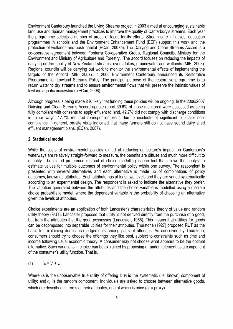
(2008a, 2008b). The range in levels was guided by flow rate data from the Environment Canterbury website (www.ecan.govt.nz) and ECan (2001). The experimental design used is an orthogonal main effects fractional factorial design constructed utilising procedures from Street and Burgess (2005). The experimental design consisted of 18 treatments which were randomly blocked into 3 blocks of 6 choice sets. Figure 1 provides an example choice set. The constant base alternative (Option 1) was assumed to be a worsening condition of rivers and streams if no change in management occurs. In the „No change‟ scenario there would be no annual cost, however it is assumed the risk of getting sick will be at its greatest, ecological quality will be poor, and the number of low-flow months will be at its highest. Figure: 1 Example choice set
Outcomes Option 1: No change
Option 2 Option 3
For every 1000 people, the number who become sick from recreational contact each year would be
60 30 10
Ecological quality of local streams and rivers Poor Good Good
Number of low flow months 5 5 1
Annual cost to Canterbury households $0 $15 $75
I would choose option 1
I would choose option 2
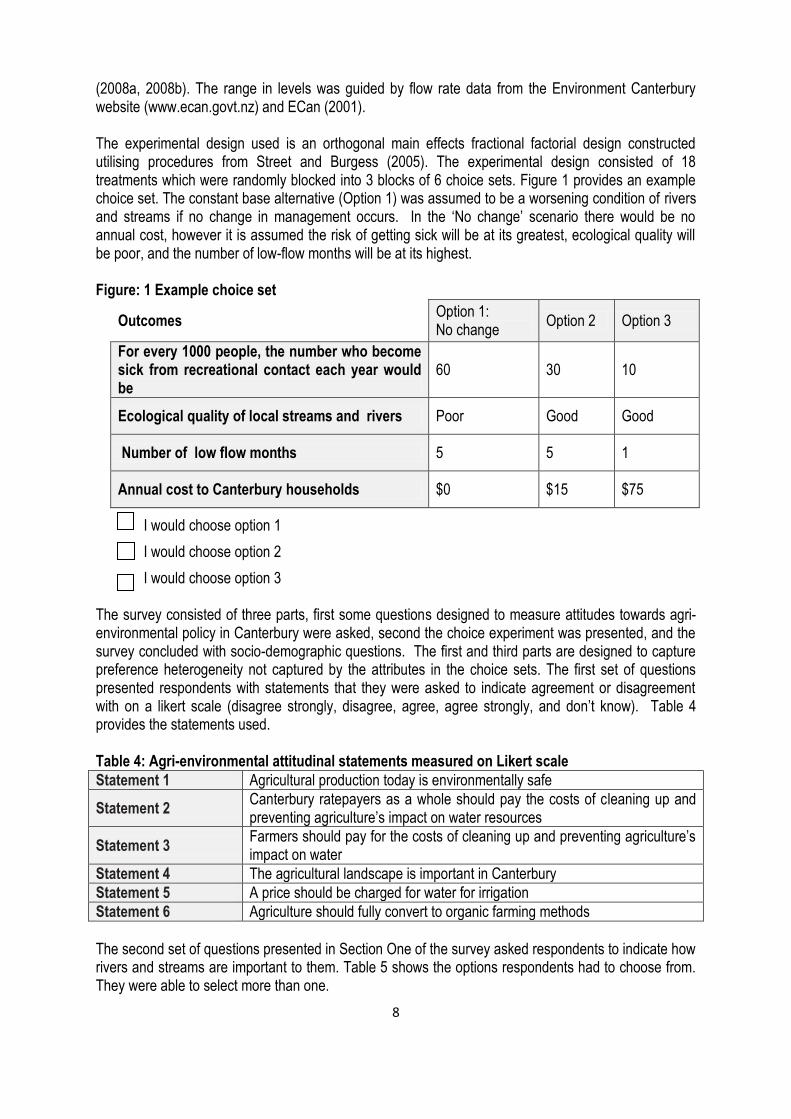
I would choose option 3 The survey consisted of three parts, first some questions designed to measure attitudes towards agri-environmental policy in Canterbury were asked, second the choice experiment was presented, and the survey concluded with socio-demographic questions. The first and third parts are designed to capture preference heterogeneity not captured by the attributes in the choice sets. The first set of questions presented respondents with statements that they were asked to indicate agreement or disagreement with on a likert scale (disagree strongly, disagree, agree, agree strongly, and don‟t know). Table 4 provides the statements used. Table 4: Agri-environmental attitudinal statements measured on Likert scale
Statement 1 Agricultural production today is environmentally safe
Statement 2 Canterbury ratepayers as a whole should pay the costs of cleaning up and preventing agriculture‟s impact on water resources
Statement 3 Farmers should pay for the costs of cleaning up and preventing agriculture‟s impact on water
Statement 4 The agricultural landscape is important in Canterbury
Statement 5 A price should be charged for water for irrigation
Statement 6 Agriculture should fully convert to organic farming methods
The second set of questions presented in Section One of the survey asked respondents to indicate how rivers and streams are important to them. Table 5 shows the options respondents had to choose from. They were able to select more than one.
9
Table 5: Importance of Canterbury rivers and streams to respondents
Importance 1 Resource for future generations
Importance 2 Recreational opportunities
Importance 3 Habitat for plants and animals
Importance 4 Resource for commercial development
Importance 5 I just like knowing that they are there
Importance 6 Drinking water resource for public
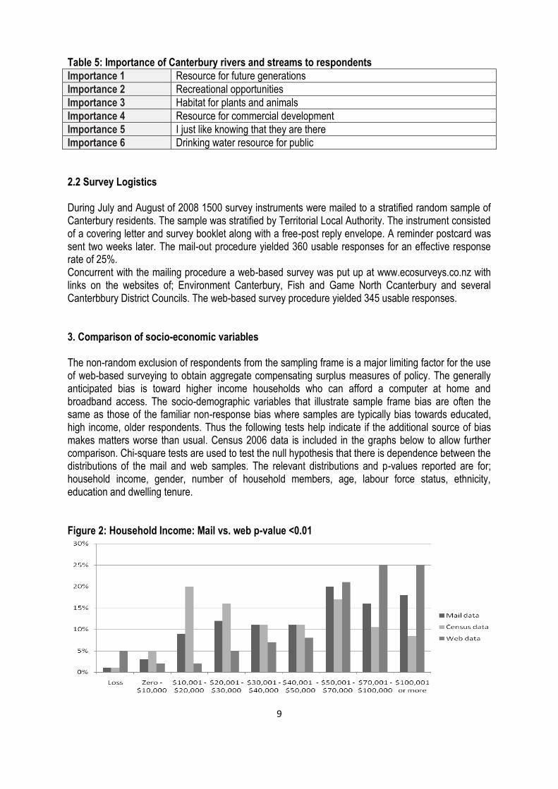
2.2 Survey Logistics During July and August of 2008 1500 survey instruments were mailed to a stratified random sample of Canterbury residents. The sample was stratified by Territorial Local Authority. The instrument consisted of a covering letter and survey booklet along with a free-post reply envelope. A reminder postcard was sent two weeks later. The mail-out procedure yielded 360 usable responses for an effective response rate of 25%. Concurrent with the mailing procedure a web-based survey was put up at www.ecosurveys.co.nz with links on the websites of; Environment Canterbury, Fish and Game North Ccanterbury and several Canterbbury District Councils. The web-based survey procedure yielded 345 usable responses. 3. Comparison of socio-economic variables The non-random exclusion of respondents from the sampling frame is a major limiting factor for the use of web-based surveying to obtain aggregate compensating surplus measures of policy. The generally anticipated bias is toward higher income households who can afford a computer at home and broadband access. The socio-demographic variables that illustrate sample frame bias are often the same as those of the familiar non-response bias where samples are typically bias towards educated, high income, older respondents. Thus the following tests help indicate if the additional source of bias makes matters worse than usual. Census 2006 data is included in the graphs below to allow further comparison. Chi-square tests are used to test the null hypothesis that there is dependence between the distributions of the mail and web samples. The relevant distributions and p-values reported are for; household income, gender, number of household members, age, labour force status, ethnicity, education and dwelling tenure. Figure 2: Household Income: Mail vs. web p-value <0.01

10
Figure 3: Gender: Mail vs. web p-value <0.01
Figure 4: Number of household members: Mail vs. web p-value = 0.847
Figure 5: Age: Mail vs. web p-value 0.968
Male Female

11
Figure 6: Labour force status: Mail vs. web p-value = 0.775
Figure 7: Ethnicity: Mail vs. web p-value <0.01
Figure 8: Education: Mail vs. web p-value 0.0121

12
Figure 9: Dwelling tenure: Mail vs. web p-value 0.07
The chi-square tests indicate that at a 1% level of significance there are differences in; Household Income with the web sample biased towards higher income; Gender with the web sample biased towards male; Ethnicity with more web respondents of New Zealand ethnicity. Differences in; Education are significant at a 5% level but not 1%; Dwelling Tenure is significant at a 10% level but not 5%. There are no significant differences between Labour Force Status, Age or Number of Household Members. Thus the results of the Socio-demographic comparisons are inconclusive as there are 3 clear-cut differences, 3 clear-cut similarities and 2 that could go either way depending on the level of significance chosen. 4. Model estimation All random parameters are specified distributed normal. Five hundred shuffled Halton draws are used in maximising the simulated Log-likelihood function. The attributes are effects coded into two variables for each attribute with the lowest level of quality being the fixed comparator for each attribute; Ecology Fair (coded 1 if Fair, 0 if Good, -1 if Poor) and Ecology Good (coded 1 if Good, 0 if Fair, -1 if Poor); Risk10 (1 if Risk10, 0 if Risk30, -1 if Risk60) and Risk30 (1 if Risk30, 0 if Risk10, -1 if Risk60); Flow1 (1 if Flow1, 0 if Flow3, -1 if Flow5), Flow3 (1 if Flow3, 0 if Flow1, -1 if Flow5). The non-attribute variables were interacted with the alternative specific constant to be included in modelling. Model variables are summarised in table 6. Table 6: Model data summary
Risk10 10 people/1000/year sick from recreational contact
Risk30 30 people/1000/year sick from recreational contact
Ecology Good Ecological quality is good
Ecology Fair Ecological quality is fair
Flow1 1 month of low-flow/year
Flow3 3 months of low-flow/year
Cost $15, $30, $45, $60, $75 and $90/household/year
ASC alternative specific constant, 1 if alternative 2 or 3, 0 if base alternative
Web 1 if answered survey online,0 if answered by mail
Perception respondent agrees that water quality is good or very good
Safe respondent agrees that agriculture is environmentally safe
Ratepayers respondent agrees that ratepayers should pay for water policy
Future respondent indicates water as future resource is important
13
Habitat respondent indicates water as habitat for plants and animals is important
Commercial respondent indicates commercial use important
Use respondent has recreational use of water
Rural respondent lives in rural area
Income household gross yearly income
Businesses respondent indicates farms are businesses and should pay for water policy
Education education level of respondent
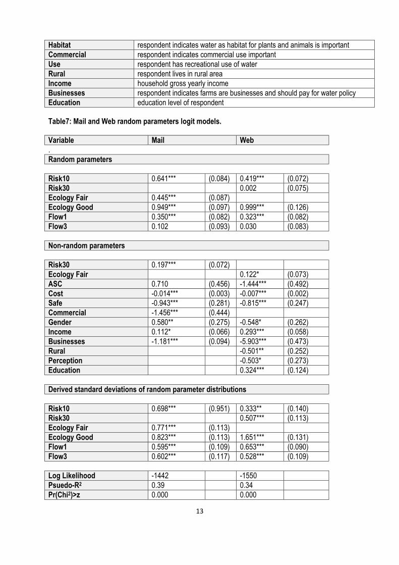
Table7: Mail and Web random parameters logit models.
Variable Mail Web
.
Random parameters
Risk10 0.641*** (0.084) 0.419*** (0.072)
Risk30 0.002 (0.075)
Ecology Fair 0.445*** (0.087)
Ecology Good 0.949*** (0.097) 0.999*** (0.126)
Flow1 0.350*** (0.082) 0.323*** (0.082)
Flow3 0.102 (0.093) 0.030 (0.083)
Non-random parameters
Risk30 0.197*** (0.072)
Ecology Fair 0.122* (0.073)
ASC 0.710 (0.456) -1.444*** (0.492)
Cost -0.014*** (0.003) -0.007*** (0.002)
Safe -0.943*** (0.281) -0.815*** (0.247)
Commercial -1.456*** (0.444)
Gender 0.580** (0.275) -0.548* (0.262)
Income 0.112* (0.066) 0.293*** (0.058)
Businesses -1.181*** (0.094) -5.903*** (0.473)
Rural -0.501** (0.252)
Perception -0.503* (0.273)
Education 0.324*** (0.124)
Derived standard deviations of random parameter distributions
Risk10 0.698*** (0.951) 0.333** (0.140)
Risk30 0.507*** (0.113)
Ecology Fair 0.771*** (0.113)
Ecology Good 0.823*** (0.113) 1.651*** (0.131)
Flow1 0.595*** (0.109) 0.653*** (0.090)
Flow3 0.602*** (0.117) 0.528*** (0.109)
Log Likelihood -1442 -1550
Psuedo-R2 0.39 0.34
Pr(Chi2)>z 0.000 0.000

14
Iterations 30 21
Observations 2160 2070
Standard errors in parenthesis; *,**,*** indicates significance at 10,5 and 1%
A Wald test of the linear restriction that the parameters of the effects coded variables are equal retained the null of inequality for all attributes. Looking at Table 7 we can see that the Chi-square tests indicate that as a whole both models are statistically significant. The Psuedo-R2 measures show that both models improve the value of the log-likelihood significantly. Looking at the attribute variables, for both models improvements in the levels of the attributes increase the probability of that option being chosen, with the magnitude of the probability increasing as the attribute level improves. In the mail-and-return model all attributes are significantly different from zero at 1% level except Flow3 which is insignificant. All attributes except Risk30 have normally distributed random parameters. In the web model Risk30 and Flow3 are insignificant and Ecology Fair is only significant at a 10% level. This indicates that web respondent preferred the highest level of policy enhancement that was offered. All attributes except Ecology Fair have normally distributed random parameters. The ASC is positive and insignificant in the mail model but is negative and highly significant in the web model. For both models higher household income increased the probability of choosing an alternative with improvements in water quality. Respondents who agreed that agriculture is environmentally safe were less likely to choose an alternative with improvements in water quality. Turning to the non-attribute variables. In the mail sample respondents who valued Canterbury rivers and streams as a commercial resource were less likely to choose a management change option. The sign of „Gender‟ switches from positive in the mail sample to negative for the web sample. Household income is positive in both models. In both samples, respondents who considered that commercial farms should pay for any policy change were less likely to choose a management change option, with the magnitude of this „Businesses‟ variable being much larger in web model. In the web sample education is positive; respondents who lived in rural areas of Canterbury were less likely to choose a management change option; respondent who thought that Canterbury streams and rivers water quality is good or very good were less likely to choose a management change option. The alternative specific constant is positive though insignificant in the mail sample, but is negative and significant for the web sample suggesting that the mail sample derives utility from a management change while the web sample does not. 4.1 Differences in Willingness-to-pay and Compensating surplus The hypotheses to be tested are: (4) H0: WTP i, Mail = WTP i, Web
H1: WTP i, Mail ≠ WTP i, Web
(5) H0: CS j, Mail = CS j, Web
H1: CS j, Mail ≠ CS j, Web
Where WTPi is the willingness-to-pay for the attribute i, and CSj is the compensating surplus for the scenario j. To test these hypotheses a parametric bootstrapping technique (Krinsky and Robb 1986) was used to draw a vector of 1000 parameter estimates from the multivariate normal distribution with mean and variance equal to the parameter mean vectors and the covariance matrix of the estimated RPL model, for each of the models. WTP measures were calculated from each parameter estimate. The simple convolutions method of Poe et al. (2001) was then used to estimate the average proportion (over 100 random draws) of WTP differences that were negative. This proportion is used to approximate a p-value for the null hypothesis of no difference between the distributions of wtp of the mail and web models. The one tailed test is for the proportion to be less than 0.05. This means that
15
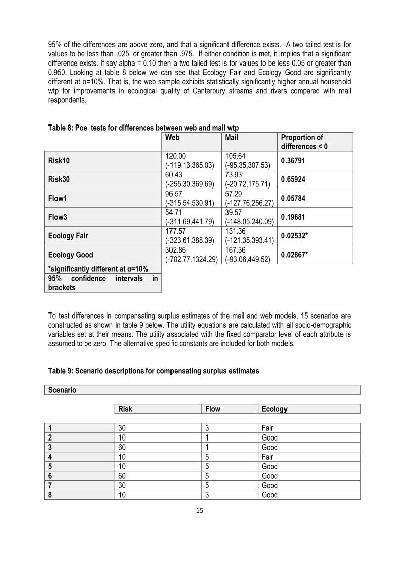
95% of the differences are above zero, and that a significant difference exists. A two tailed test is for values to be less than .025, or greater than .975. If either condition is met, it implies that a significant difference exists. If say alpha = 0.10 then a two tailed test is for values to be less 0.05 or greater than 0.950. Looking at table 8 below we can see that Ecology Fair and Ecology Good are significantly different at α=10%. That is, the web sample exhibits statistically significantly higher annual household wtp for improvements in ecological quality of Canterbury streams and rivers compared with mail respondents. Table 8: Poe tests for differences between web and mail wtp
Web Mail Proportion of differences < 0
Risk10 120.00 (-119.13,365.03)
105.64 (-95.35,307.53)
0.36791
Risk30 60.43 (-255.30,369.69)
73.93 (-20.72,175.71)
0.65924
Flow1 96.57 (-315.54,530.91)
57.29 (-127.76,256.27)
0.05784
Flow3 54.71 (-311.69,441.79)
39.57 (-148.05,240.09)
0.19681
Ecology Fair 177.57 (-323.61,388.39)
131.36 (-121.35,393.41)
0.02532*
Ecology Good 302.86 (-702.77,1324.29)
167.36 (-93.06,449.52)
0.02867*
*significantly different at α=10%
95% confidence intervals in brackets
To test differences in compensating surplus estimates of the mail and web models, 15 scenarios are constructed as shown in table 9 below. The utility equations are calculated with all socio-demographic variables set at their means. The utility associated with the fixed comparator level of each attribute is assumed to be zero. The alternative specific constants are included for both models. Table 9: Scenario descriptions for compensating surplus estimates
Scenario
Risk Flow Ecology
1 30 3 Fair
2 10 1 Good
3 60 1 Good
4 10 5 Fair
5 10 5 Good
6 60 5 Good
7 30 5 Good
8 10 3 Good

16
9 30 1 Fair
10 60 3 Poor
11 30 5 Poor
12 10 3 Poor
13 10 1 Poor
14 30 1 Poor
15 10 3 Fair
The Poe test results shown in table 10 show that there are no statistically significant differences in any of the compensating surplus estimates between the web and mail samples.
Table 10: Poe tests for differences between web and mail compensating surplus estimates
Scenario Individual mean Compensating Surplus
Web Mail proportion of differences < 0
1 72.64
(-290.18, 144.90) 144.01
(8.33,288.48) 0.31
2 327.09
(-859.76, 205.58 228.89
(51.75, 406.04) 0.59
3 264.73
(-790.05, 260.58) 181.03
(37.20, 324.87) 0.57
4 134.10
(-36.83, -231.36) 170.82
(20.37, 321.26) 0.35
5 253.24
(-247.23,753.71) 203.83
(50.28,357.38) 0.75
6 189.77
(-299.72,679.68) 120.12
(10.01,230.22) 0.27
7 191.94
(-313.94,696.42) 174.04
(56.37,291.71) 0.41
8 257.73
(-272.45,788) 209.88
(34.28,385.49) 0.47
9 123.68
(-127.83,375.21) 160.89
(27.01,294.78) 0.32
10 57.7
(-214.42,98.98) 94.71
(8.71,180.54) 0.43
11 54.69
(-204.01,94.61) 103.04
(22.35,170.23) 0.72
12 121.18
(-68.19,310.57) 138.89
(9.24,268.55) 0.81
13 167.17
(-55.46,389.81) 159.15
(28.33,289.96) 0.62
14 105.17
(-146.34,356.69) 129.35
(42.95,215.73) 0.43
15 139.7
(-49.68,329.09) 170.44
(2.07,342.95) 0.38
95% confidence intervals in brackets

17
4.2 Pooled Model Another approach to examine possible differences between web and mail samples is to estimate a pooled model with a dummy variable equal to 1 if the respondent uses the web mode. The pooled model is estimated from the stacked web and mail data set.
Table 11: Random parameters logit model: Pooled data
Variable Coeff. s.e Coeff./s.e. P-value
.
Random parameters
Flow1 0.327 0.057 5.768 0.000
Ecology Good 0.947 0.075 12.670 0.000
Non-random parameters
ASC 0.093 0.280 0.334 0.738
Ecology Fair 0.224 0.045 4.889 0.000
Flow3 -0.055 0.049 -1.132 0.257
Risk10 0.462 0.043 10.637 0.000
Risk30 0.137 0.043 3.162 0.002
Cost -0.008 0.002 -5.085 0.000
Web -2.229 0.184 -12.107 0.000
Commercial -1.674 0.395 -4.237 0.000
Safe -0.819 0.158 -5.182 0.000
Income 0.202 0.036 5.542 0.000
Education 0.234 0.081 2.913 0.036
Businesses -1.516 0.104 -14.456 0.000
Derived standard deviations of parameter distributions
Ecology Good 1.333 0.073 18.278 0.000
Flow1 0.780 0.055 14.098 0.000
Log Likelihood -3169
Psuedo-R2 0.34
Pr(Chi2)>z 0.0000
Iterations 29
Observations 4230
Looking at Table 11 above we can see that the binary variable Web is highly significant and negative indicating that the probability of the respondent choosing an enhanced management option is lowered if the respondent completed the survey online. This result may reflect the fact that more web respondents choose the no change option compared to the mail respondents, 19% of the web respondents choose the no change option compared to 8% of mail respondents. In general the pooled data model seems to perform no better than either the web or mail data models.

18
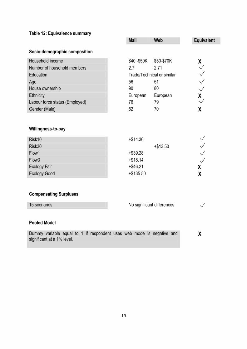
5. Discussion The purpose of this paper was to compare choice experiment data from two survey modes, traditional mail-and-return, and web-based. In terms of sample socio-demographic composition the web and mail samples are the same for Labour Force Status, Age and Number of Household Members but are different for Household Income, Gender and Ethnicity. Education and Dwelling Tenure are not statistically different at a 1% level. This would look like a tie depending on which variables were thought to be important. Poe tests reveal that there are significant differences in wtp for ecological improvements with the web sample having higher mean wtp. There are no differences detected for all other attribute wtp estimates. Poe tests also reveal that there are no differences detected for compensating surplus estimates over 15 scenarios. A pooled model with a dummy variable equal to 1 if respondent uses web mode is specified and is found to be negative and statistically significant at a 1% level suggesting that there is some unobserved source of heterogeneity between the web and mail sample that is omitted from the model. Although web respondents place a lot of value on the „Ecology‟ attribute, they have a higher WTP for this attribute and a higher CS for all scenarios that involve „Ecology Good‟, yet overall the Web variable is highly significant and negative. Why are they less willing to chose a „change‟ option if they value the ecological variable so highly? This raises the possibility that the „Ecology‟ attribute is more of a pure public-good attribute than the others-which are more reflective of direct use. This suggests that web respondents value the environment but don‟t want to pay for it. Table 12 below provides a summary of findings for the three approaches used to assess whether traditional mail and web-based survey modes provide equivalent results to the nonmarket valuation practitioner. Averages are reported for demographic variables while differences are given for wtp estimates. A cross indicates that they do not produce the same results while a tick indicates that the two survey modes produce the same results. Overall this paper has demonstrated that samples collected via the internet and traditional mail and return samples are not drastically different. This finding supports the conclusion that non-market valuation practitioners seeking to take advantage of web-based surveying will not jeopardise the validity and reliability of their results.
19
Table 12: Equivalence summary
Socio-demographic composition
Mail Web Equivalent
Household income $40 -$50K $50-$70K X
Number of household members 2.7 2.71
Education Trade/Technical or similar
Age 56 51
House ownership 90 80
Ethnicity European European X
Labour force status (Employed) 76 79
Gender (Male) 52 70 X
Willingness-to-pay
Risk10 +$14.36
Risk30 +$13.50
Flow1 +$39.28
Flow3 +$18.14
Ecology Fair +$46.21 X Ecology Good +$135.50 X
Compensating Surpluses
15 scenarios No significant differences
Pooled Model
Dummy variable equal to 1 if respondent uses web mode is negative and significant at a 1% level.
X

20
References
Adamowicz, W.; Dupoint, D.;Krupnik and Zhang, J. (2007). Valuation of Cancer and Microbial Risk Reductions in Municipal Drinking Water: An Analysis of Risk Context Using Multiple Valuation Methods. Resources for the Future, Washington, DC, available at www.rff.org.
Ball. A. (2006). Estimation of the Burden of Water-Borne Disease in New Zealand: Preliminary Report. New Zealand Ministry of Health
Berrens, R., Bohara, A., Jenkins-Smith, H., Silva, C. and Weimer, D. (2004). “Information and effort in contingent valuation surveys: Application to global climate change using national Internet samples.” Journal of Environmental Economics and Management, 47(2): 331-363.
Berrens, R., Bohara, A., Jenkins-Smith, H., Silva, C. and Weimer, D. (2003). “The advent of Internet surveys for political research: A comparison of telephone and Internet samples.” Political Analysis, 11(1): 1-22.
Bewsell, D. and Kaine, G. (2005). “Adoption of Environmental Bet Practice Amongst Dairy Farmers”. Paper presented at the Eleventh Annual Conference of the New Zealand Agricultural and Resource Economics Society (Inc.). AERU Discussion Paper No. 152.
Cameron, K. C. and Di, H. J. (2004). Nitrogen leaching losses from different forms and rates of farm effluent applied to a Templeton soil in Canterbury, New Zealand. New Zealand Journal of Agricultural Research, vol. 47, pp. 429-37.
Cameron, K. C.; Di, H. J.; Reijnen, B. P. A.; Li, Z.; Russell, J. M. and Barnett, J. W. (2002). Fate of nitrogen in dairy farm factory effluent irrigated onto land. New Zealand Journal of Agricultural Research, vol. 45, pp. 207-16.
Cole, S. T.(2005). “Comparing Mail and Web-based Survey Distribution Methods: Results of Surveys to Leisure Travel Retailers”. Journal of Travel Research, 43:422-430.
Dillman, Don A. Mail and Internet Surveys: The Tailored Design Methods. New York: John Wiley and Sons, 2000.
Dickie, M.; Gerking, S. and Goffe, W.J. (2007). Valuation of non-market goods using computer-assisted surveys: a comparison of data quality from internet and rdd samples. Available at http://goffe.oswego.edu/Survey_Comparison_3.pdf.
Deutskens, E.; Ruyter, K. D. And Wetzels, M. (2006). “An Assessment of Equivalence Between Online and Mail Surveys in Service Research.” Journal of Service Research, 8(4): 346-355.
Dillman, D. A. (2007). Mail and Internet Surveys the Tailored Design Method. Hoboken, N.J.: Wiley, c2007.
Environment Canterbury. (2008) The Restorative Programme for Lowland Streams. Available at www.ecan.govt.nz.
Environment Canterbury. (2001). Our water in the balance: Christchurch West Melton rivers and groundwater, issues and options. Environment Canterbury Report R01/1.
Environment Canterbury. (2003). Ecosystem health of Canterbury rivers: Development and implementation of biotic and habitat assessment methods 1999/2000. Report No. R03/3.
Environment Canterbury (2007). NRRP Hearing stage 12 Officer Report No.12 Chapter 4 WQL2 on Proposed Variation 1 of the Proposed Canterbury Natural Resources Regional Plan: Chapter 4 – Water Quality – Submissions on Issue WQL1, Objective WQL1.1 & 1.2, Policies WQL1, WQL2, WQL3 & WQL5. Environment Canterbury, (2007b). Freshwater contact recreational monitoring programme summary report 2006/2007.
Environment Canterbury.(2007a). The compliance status of dairy shed effluent discharges to land in the Canterbury region for the 2006/2007 season. Report No. R07/23.
Environment Canterbury (2007b) Project Outputs and Funding for 2005-2006. Available at www.ecan.govt.nz.
Fleming, C. M. and Bowden, M. (2009). Web-based surveys as an alternative to traditional mail methods. Journal of Environmental Management 90: 284-292.

21
Griffis, S. E.; Goldsby, T. J and Cooper, M. (2003). “Web-based and Mail Surveys: a Comparison of Response, Data and Cost”. Journal of Business Logistics, 12(2): 237-258.
Hamill, K. D. and McBride, G. B. (2003). River water quality trends and increased dairying in Southland, New Zealand. New Zealand Journal of Marine and Freshwater Research, vol. 37, pp. 323-332
Hausman, J. and McFadden, D. (1984). Specification tests for the multinomial logit model. Econometrica, 52: 1219-1240.
Krinsky, I. and Robb, A. L. (1986). On approximating the statistical properties of elasticities. Review of Economics and Statistics 68: 715–719.
Krosnick, Jon A. and LinChiat Chang. 2004. “National Surveys Via RDD Telephone Interviewing vs. the Internet: Comparing Sample Representativeness and Response Quality,” Center for Survey Research, Ohio State University.
Lancaster, K. (1966). A New Approach to Consumer Theory. Journal of Political Economy, 74: 132-157. Larned, S. T.; Scarsbrook, M. R.; Snelder, T. H.; Norton, N. J. and Briggs, B. J. F. (2004).Water quality
in low-elevation streams and rivers of New Zealand: recent state and trends in contrasting land-cover classes. New Zealand Journal of Marine and Freshwater Research, vol. 38, pp. 347-66.
Lindhjem, Henrik and Navrud, Stale,Internet CV Surveys - A Cheap, Fast Way to Get Large Samples of Biased Values?(April 15, 2008). Available at SSRN: http://ssrn.com/abstract=1295521
McBride G; Till D; Ryan T; Ball A; Lewis G; Palmer S; Weinstein P. (2002). Freshwater Microbiology Research Programme. Pathogen occurrence and human health risk assessment analysis. Ministry for the Environment & Ministry of Health, Wellington.ealands Clean Green Image. Available at www.mfe.govt,nz.
Ministry for the Environment (2008a). Draft Guidelines for the Selection of Methods to Determine Ecological Flows and Water Levels. Available at www.mfe.govt.nz
Ministry for the Environment (2008b) Flow Guidelines for Instream Values. Available at www.mfe.govt.nz
Ministry for the Environment, (2003). Dairying and Clean Streams Accord. Available at www.mfe.govt.nz.
Ministry for the Environment, (2007). The Dairying and Clean Streams Accord: Snapshot of Progress-2005/2006. Available at www.mfe.govt.nz.
Parliamentary Commissioner for the Environment (PCE). 2004. Growing for good: Intensive farming, sustainability and New Zealand‟s environment. Wellington: Parliamentary Commissioner for the Environment.
Poe, G. L., K. L. Giraud and J. B. Loomis. (2001). Simple Computional Methods for Measuring the Differences of Empirical Distributions: Application to Internal and External Scope Tests in Contingent Valuation, Staff Paper 2001-05, Department of Agricultural, Resource and Managerial Economics, Cornell University
Ready, R.; Fisher, A.; Guignet, D.; Stedman, R. and Wang, J. (2006) “A pilot test of a new stated preference valuation method: Continuous attribute-based stated choice”. Ecological Economics, 59: 247-255
Ross, C. and Donnison, A. (2003). Campylobacter and farm dairy effluent irrigation.”New Zealand Journal of Agricultural Research, vol. 46, pp 255-62.
Ross, C. and Donnison, A. (2004).Survival of Campylobacter jejuni in soil after farm dairy effluent irrigation”. In: Wang, H.; Lavery, J. M. ed. Water, waste and land treatment for primary industry and rural areas. Proceedings of the 2004 New Zealand land Treatment Collective Annual Conference, Ashburton, New Zealand, pp. 102-08
Saggar, S.; Bolan, N. S.; Bhandral, R.; Hedley, C.; Luo, J.(2004). A review of emissions of methane, ammonia and nitrous oxide from animal excreta depositionand farm effluent application in grazed pastures. New Zealand Journal of Agricultural Research 47: 513–544.
Stark, J.D. (1998). SQMCI: a biotic index for freshwater macroinvertebrate coded-abundance data. New Zealand Journal of Marines and Freshwater Research, 32:55-66.

22
Stark, J.D. and Maxted, J.R. (2007). A biotic index for New Zealand‟s soft-bottomed streams. New Zealand Journal of Marines and Freshwater Research, 41:43-61.
Stark, J.D. and Maxted J.R. (2007b). A user guide for the Macroinvertebrate Community Index. Prepared for the Ministry for the Environment. Cawthron Report No.1166. 58 p.
Statistics New Zealand (2007). Agricultural Statistics New Zealand. www.stats.govt.nzUTH Thurstone, L. L. (1927). A Law of Comparative Judgement. Psychological Review, 34: 273-86. Tsuge, T. and Washida, T. (2003). “Economic valuation of the Seto Inland Sea using an Internet CV
survey”. Marine Pollution Bulletin, 47: 230-236. van der Heide, C. M., van den Bergh, J., van Ierland, E. and Nunes, P. (2005). “Measuring the
economic value of two habitat defragmentation policy scenarios for the Veluwe, The Netherlands.” Fondazione Eni Enrico Mattei Working Paper No. 42, Milan.
von Stackelberg, Katharine and James K. Hammitt. 2006. “Use of Contingent Valuation to
Elicit Willingness-to-Pay for the Benefits of Developmental Health Risk Reductions,” Harvard University, Center for Risk Analysis working paper.
Wang. H. And Magesan. G. N. (2004). An overview of the environmental effects of land application of farm effluents. New Zealand Journal of Agricultural Research v.47:289-403.
Whittaker, D., J. J. Vaske, M. P. Donnelly, and D. S. De Ruiter. 1998. “Mail Versus TelephoneSurveys: Potential Biases in Expenditure and Willingness-to-Pay,” Journal of Park and Recreational Administration 16: 15-30.