Embed Size (px)
Citation preview

M. J. Roberts - 2/18/07
P-1
Web Appendix P - Complex Numbers andComplex Functions
P.1 Basic Properties of Complex Numbers
In the history of mathematics there is a progressive broadening of the concept of“numbers”. The first numbers were the natural counting numbers, 1,2,3… Next werezero and the negative numbers completing the set we now call integers. Fractions (ratiosof integers) filled in some of the points between integers and later irrational numbersfilled in all the gaps between fractions to form what we now call the real numbers, aninfinite continuum of one-dimensional numbers.
In trying to solve quadratic equations of the form ax2
+ bx + c = 0 real solutions
can always be found if b2
4ac is greater than or equal to zero. But if b2
4ac is lessthan zero, no real solution can be found. The essence of the problem is in trying to solve
the equation x2
= 1 for x. None of the real numbers can be the solution of this equation.The proposal that an imaginary number could be the solution to this equation led to awhole new field of mathematics, complex variables. The idea of complex numbersseemed artificial and abstract at first but as mathematical and physical theory hasdeveloped, the usefulness of complex numbers solving practical problems has beenconclusively shown. The square root of minus one has been given the symbol j and
therefore j
2= 1 .
________________________________________________________________________
Different authors use different symbols to indicate the square root of minus one. Acommonly-used symbol is i. This is used in many mathematics and physics books. Thesymbol j is preferred in most electrical engineering books to avoid confusion because thesymbol i is usually reserved for electrical current.________________________________________________________________________
A complex number z can be expressed as the sum of a real number x and animaginary number jy where y is also a real number. In the complex number z = x + jy , xis the real part and y is the imaginary part. (Notice that, although it sounds strange, theimaginary part of a complex number is a real number.) Two complex numbers are equalif, and only if, their real and imaginary parts are equal separately.
Let z
1= x
1+ jy
1and z
2= x
2+ jy
2. Then, if
z
1= z
2that implies that
x
1= x
2and y
1= y
2.
In the following material the symbol z will represent some arbitrary complex number andthe symbols x and y will represent the real and imaginary parts of z respectively.
The sum and product of two complex numbers are defined as
z
1+ z
2= x
1+ jy
1( ) + x
2+ jy
2( ) = x
1+ x
2+ j y
1+ y
2( ) (P.1)

M. J. Roberts - 2/18/07
P-2
and
z
1z
2= x
1+ jy
1( ) x
2+ jy
2( ) = x
1x
2y
1y
2+ j x
1y
2+ x
2y
1( ) . (P.2)
From (P.1),
z + 0 = z + 0 + j0( ) = x + 0( ) + j y + 0( ) = x + jy = z
proving that the number, zero, is the additive identity for complex numbers just as it is forreal numbers. From (P.2),
z 1 = z 1+ j0( ) = x 1( ) y 0( )( ) + j x 0( ) + y 1( )( ) = x + jy = z
proving that the real number 1 is the multiplicative identity for complex numbers, just as itis for real numbers.
By a straightforward extension of the law of addition, subtraction is defined by
z
1z
2= x
1x
2+ j y
1y
2( ) .
Division can be derived from multiplication and the result is
z1
z2
=x
1x
2+ y
1y
2
x2
2+ y
2
2+ j
x2y
1x
1y
2
x2
2+ y
2
2= x
3+ jy
3= z
3
It follows that
z
z= 1 ,
z1
z2
= z1
1
z2
and1
z1z
2
=1
z1
1
z2
, z1
0 , z2
0( ) .

M. J. Roberts - 2/18/07
P-3
________________________________________________________________________
Example P-1 Adding, subtracting, multiplying and dividing complex numbers withMATLAB
3+ j2( ) + 1+ j6( ) = 2 + j8 ,
3+ j2( ) 1+ j6( ) = 4 j4
3+ j2( ) 1+ j6( ) = 15 + j16 ,
3+ j2
1+ j6=
9
37j20
37
MATLAB handles complex numbers just as easily as real numbers. These fournumerical calculations can be done by MATLAB directly at the computer console in theinteractive mode. Below is a copy of a MATLAB session doing these calculations.
»A = 3 + j*2 ; B = -1+j*6 ;
»A + B
ans =
2.0000 + 8.0000i
»A - B
ans =
4.0000 - 4.0000i
»A*B
ans =
-15.0000 +16.0000i
»A/B
ans =
0.2432 - 0.5405i
The square root of minus one is predefined in MATLAB and is the default value of thevariables i and j.________________________________________________________________________
The commutativity and associativity of complex numbers under addition andmultiplication,
z
1+ z
2= z
2+ z
1, z
1+ z
2+ z
3( ) = z1+ z
2( ) + z3
(P.3)
and
z
1z
2= z
2z
1, z
1z
2z
3( ) = z1z
2( ) z3 , (P.4)
and the distributivity of complex numbers,
z
1z
2+ z
3( ) = z
1z
2+ z
1z
3 , (P.5)
can be proven from the definition of complex numbers and the commutativity,associativity and distributivity of real numbers. These properties (P.3), (P.4) and (P.5)lead to the results
M. J. Roberts - 2/18/07
P-4
z1+ z
2
z3
=z
1
z3
+z
2
z3
andz
1z
2
z3z
4
=z
1
z3
z2
z4
, z3
0 , z4
0( ) .
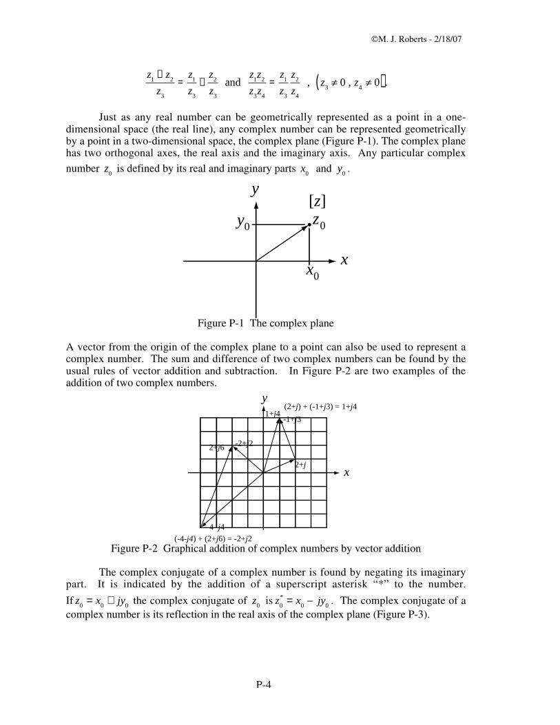
Just as any real number can be geometrically represented as a point in a one-dimensional space (the real line), any complex number can be represented geometricallyby a point in a two-dimensional space, the complex plane (Figure P-1). The complex planehas two orthogonal axes, the real axis and the imaginary axis. Any particular complex
number z
0 is defined by its real and imaginary parts
x
0 and
y
0.
x
y[z]z0y0
x0
Figure P-1 The complex plane
A vector from the origin of the complex plane to a point can also be used to represent acomplex number. The sum and difference of two complex numbers can be found by theusual rules of vector addition and subtraction. In Figure P-2 are two examples of theaddition of two complex numbers.
x
y(2+j) + (-1+j3) = 1+j4
(-4-j4) + (2+j6) = -2+j2
2+j
-1+j3
-4- j4
-2+j22+j6
1+j4
Figure P-2 Graphical addition of complex numbers by vector addition
The complex conjugate of a complex number is found by negating its imaginarypart. It is indicated by the addition of a superscript asterisk “*” to the number.
If z
0= x
0+ jy
0 the complex conjugate of
z
0 is
z
0
*= x
0jy
0. The complex conjugate of a
complex number is its reflection in the real axis of the complex plane (Figure P-3).

M. J. Roberts - 2/18/07
P-5
x
y[z]
z0
-y0
y0
x0z0*
Figure P-3 Complex conjugates
Some properties of conjugates that can be derived from earlier properties of complexnumbers are
z1+ z
2( )*
= z1
*+ z
2
*, z
1z
2( )*
= z1
*z
2
*, z
1z
2( )*
= z1
*z
2
*,
z1
z2
*
=z
1
*
z2
*
Also the sum of any complex number and its conjugate is real, and the difference betweenany complex number and its conjugate is imaginary.
The absolute value z (or magni tude or modulus) of a complex number,
z = x + jy , is the length of the vector in the complex plane which represents z, which is
(from the Pythagorean theorem) z = x
2+ y
2 .
Pythagoras of Samos, 569 BC – 475 BC
By extension, the distance between any two complex numbers z
1and
z
2 in the complex
plane is
z
1z
2= x
1x
2( )
2
+ y1
y2
( )2
.

M. J. Roberts - 2/18/07
P-6
The magnitude of a complex number is a real number z = x
2+ y
2+ j0 . A handy
relation in the study of complex variables and functions of a complex variable is
z
2
= zz*
= x2
+ y2 . Also,
z
1z
2= z
1z
2 ,
z1
z2
=z
1
z2
.
P.2 The Polar Form
It is often convenient in analysis to represent a complex number in polar form.Instead of specifying its real and imaginary parts, we specify its magnitude r and theangle that its vector representation in the complex plane makes with the positive realaxis, with the counter-clockwise direction being positive. The relations are
x = r cos( ) and y = r sin( ) and
z = r cos( ) + j sin( ) .
The length of the vector r is the magnitude of the complex number r = z and the angle
or phase is related to x and y by tan( ) = y / x (Figure P-4).
x
y[z]z0r0
θ0
Figure P-4 The polar form of a complex number
There is more than one value of that satisfies tan( ) = y / x , therefore the angle or
phase of a complex number is multiple valued. If is a solution, so is + 2n where n isany integer. One special case is worthy of note; the case
x = y = 0 . In this case, the ratio
y / x is undefined. That means that tan( ) = y / x and, by implication, are also
undefined. The phase of a complex number whose magnitude is zero is undefined. Thisshould not be cause for alarm. If the magnitude is zero, the vector from the origin of thecomplex plane to the complex number is a zero-length vector, or a point, the origin.Geometrically the angle from the positive real axis to this vector has no meaning becausethe vector has no length and therefore, no direction. Also, since the real and imaginary
parts of the complex number are found from x = r cos( ) and y = r sin( ) , if r is zero, x

M. J. Roberts - 2/18/07
P-7
and y are also zero regardless of the value of . So the mathematics is telling ussomething logical (as it usually does). If the magnitude is zero, phase has no meaning!
The product of two complex numbers, written in polar form, is
z
1z
2= r
1cos
1( ) + j sin
1( ) r
2cos
2( ) + j sin
2( )
z
1z
2= r
1r
2cos
1( )cos
2( ) sin
1( )sin
2( ) + j cos
1( )sin
2( ) + sin
1( )cos
2( ){ }
z1z
2=
r1r
2
2
cos1 2
( ) + cos1+
2( ) cos
1 2( ) cos
1+
2( )
+ j sin2 1
( ) + sin2
+1
( ) + sin1 2
( ) + sin1+
2( )
z
1z
2= r
1r
2cos
1+
2( ) + j sin
2+
1( )
The magnitude of the product of two complex numbers is the product of their magnitudesand the angle of the product of two complex numbers is the sum of their angles. Applyingthis idea to the product of multiple complex numbers leads to De Moivre’s theorem
z
n= r
ncos n( ) + j sin n( ) .
It also follows that the magnitude of the quotient of two complex numbers is the quotientof their magnitudes and the angle of the quotient of two complex numbers is the differenceof their angles
z1
z2
=r1
r2
cos1 2( ) + j sin
1 2( ) , r2
0 .
Abraham de Moivre, 5/26/1667 - 11/27/1754________________________________________________________________________
Example P-2 Polar-to-rectangular and rectangular-to-polar number conversions

M. J. Roberts - 2/18/07
P-8
9 + j7 = 11.4 cos 0.661( ) + j sin 0.661( ) or 11.4 0.661 or 11.4 37.87°
4 + j8 = 8.94 cos 2.034 + j sin 2.034( )( ) or 8.94 2.034or 8.94 116.57°
9 + j7( ) 4 + j8( ) = 11.4 cos 0.661( ) + j sin 0.661( ) 8.94 cos 2.034( ) + j sin 2.034( )
9 + j7( ) 4 + j8( ) = 11.4 8.94 cos 0.661+ 2.034( ) + j sin 0.661+ 2.034( )
9 + j7( ) 4 + j8( ) = 101.98 cos 2.695( ) + j sin 2.695( ) = 92 + j44
9 + j7
4 + j8=
11.4 cos 0.661( ) + j sin 0.661( )8.94 cos 2.034( ) + j sin 2.034( )
=11.4
8.94cos 0.661 2.034( ) + j sin 0.661 2.034( )
9 + j7
4 + j8= 1.275 cos 1.373( ) + j sin 1.373( ) =
1
4j5
4
In MATLAB,
»A = 9+j*7 ; B = -4+j*8 ;
»abs(A)
ans =
11.4018
»angle(A)
ans =
0.6610
»abs(B)
ans =
8.9443
»angle(B)
ans =
2.0344
»A*B
ans =
-92.0000 +44.0000i
»abs(A*B)
ans =
101.9804
»angle(A*B)
ans =
2.6955
»A/B
ans =
0.2500 - 1.2500i
M. J. Roberts - 2/18/07
P-9
»abs(A/B)
ans =
1.2748
»angle(A/B)
ans =
-1.3734________________________________________________________________________
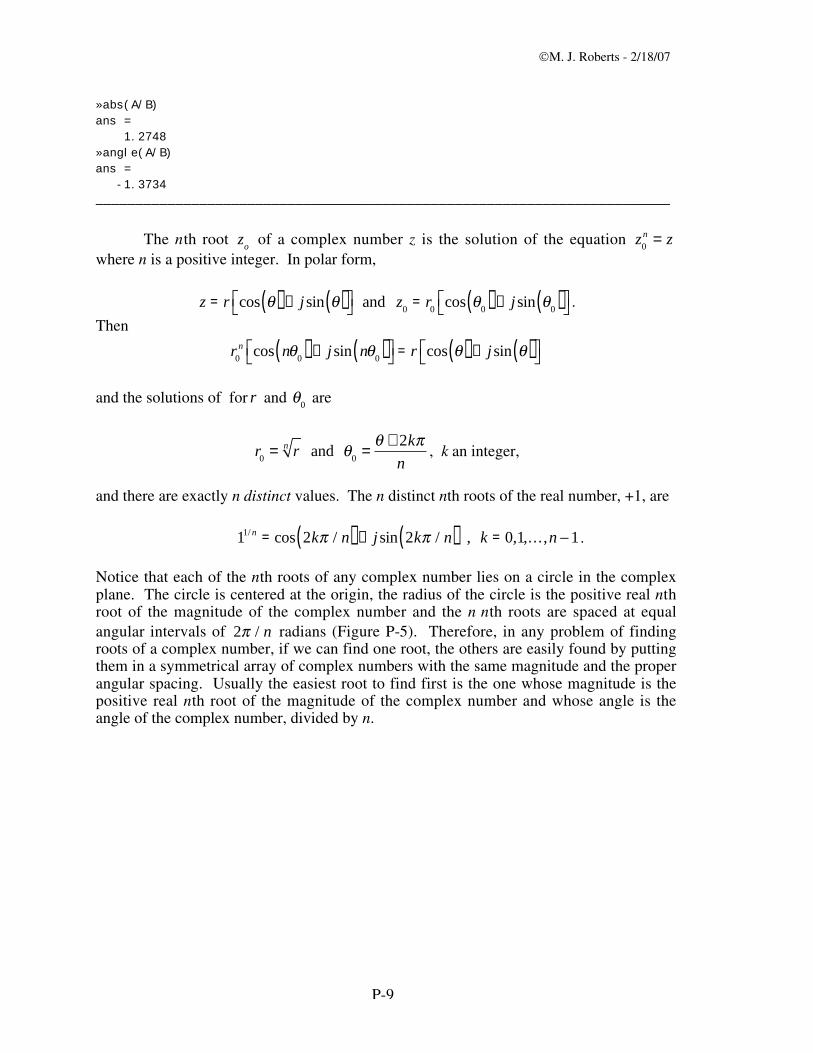
The nth root z
o of a complex number z is the solution of the equation
z
0
n= z
where n is a positive integer. In polar form,
z = r cos( ) + j sin( ) and z
0= r
0cos
0( ) + j sin
0( ) .
Then
r0
ncos n
0( ) + j sin n
0( ) = r cos( ) + j sin( )
and the solutions of for r and 0
are
r0
= rn
and0
=+ 2k
n, k an integer,
and there are exactly n distinct values. The n distinct nth roots of the real number, +1, are
1
1/ n= cos 2k / n( ) + j sin 2k / n( ) , k = 0,1,…,n 1 .
Notice that each of the nth roots of any complex number lies on a circle in the complexplane. The circle is centered at the origin, the radius of the circle is the positive real nthroot of the magnitude of the complex number and the n nth roots are spaced at equalangular intervals of 2 / n radians (Figure P-5). Therefore, in any problem of findingroots of a complex number, if we can find one root, the others are easily found by puttingthem in a symmetrical array of complex numbers with the same magnitude and the properangular spacing. Usually the easiest root to find first is the one whose magnitude is thepositive real nth root of the magnitude of the complex number and whose angle is theangle of the complex number, divided by n.

M. J. Roberts - 2/18/07
P-10
-4x
y
[z](-4)
2
2- 2
- 2
14
x
y
[z](-j)
13
1
1
-1
-1Figure P-5 Roots of complex numbers
MATLAB has a function for finding the roots of an equation roots. If theequation is of the form
a
nz
n+ a
n 1z
n 1+ a
2z
2+ a
1z + a
0= 0 , (P.6)
then the MATLAB command r o o t s ( [ a
na
n 1a
2a
1a
0] ) or
roots([ a
n,a
n 1, a
2,a
1,a
0]) or roots([
a
n;a
n 1; a
2;a
1;a
0]) returns all the distinct
roots of (P.6). For example,
»roots([3 2])
ans =
-0.6667
or
»roots([9,1,-3,6])
ans =
-1.0432
0.4661 + 0.6495i
0.4661 - 0.6495i
or
»roots([2 ; j*3 ; 1 ; -9])
ans =
-0.6573 - 2.1860i -0.7464 + 1.1162i

M. J. Roberts - 2/18/07
P-11
1.4037 - 0.4301i
P.3 Functions of a Complex Variable
In the study of signals and systems, probably the most important of the functionsof a complex variable is the exponential function, defined as
exp z( ) = e
x cos y( ) + j sin y( ) . (P.7)
Common nomenclature in signal and system analysis is that the exponential function of acomplex variable is called a complex exponential. Note that if
y = 0 in (P.7), z becomesreal and this definition collapses to the more familiar definition of the exponential function
for real variables exp z( ) = exp x( ) = e
x . If z is purely imaginary in (P.7) x = 0 and
exp jy( ) = cos y( ) + j sin y( ) .
This is known as Euler’s (pronounced “oilers”) identity after Leonhard Euler one of thegreat early mathematicians.
Leonhard Euler, 4/15/1707 - 9/18/1783
The most common occurrences of the complex exponentials in signal and system theoryare with either time t or cyclic frequency f or radian frequency as the independent variable, forexample
x t( ) = 24e 0
j0( )t
or X f( ) = 5ej2 ft
0 or X j( ) = 3e j4
where o
, 0
and t0 are real constants. When the argument of the exponential function is purely
imaginary, the resulting complex exponential is called a complex sinusoid because it contains acosine and a sine as its real and imaginary parts as illustrated in Figure P-6 for a complexsinusoid in time. The projection of the complex sinusoid onto a plane parallel to the planecontaining the real and t axes is the cosine function and the projection onto a plane parallel to theplane containing the imaginary and t axes is the sine function.

M. J. Roberts - 2/18/07
P-12
A
A
-A
-A
Re
Im
t
Ae = j2πf t0 Ae jω t0
T0
2T0
3T0
0 0Asin(2πf t) = Asin(ω t)
0 0Acos(2πf t) = Acos(ω t)
T = = 00f1
0ω2π
Figure P-6 Relation between a complex sinusoid and a real sine and a real cosine
Other important properties of the exponential function are
exp z1( )
exp z2( )
= exp z1
z2( ) ,
exp z( )
n
= exp nz( )
exp z( )m
n = expm
nz + j2k( ) , k = 0,1, n 1
The exponential function is periodic with period j2 . That is, it is periodic in theimaginary dimension . This is shown from the definition, (P.7), by substituting
z + j2n
for z
exp z + j2n( ) = e
x cos y + 2n( ) + j sin y + 2n( ) = ex cos y( ) + j sin y( ) = exp z( )
n an integer. Also exp z
*( ) = exp z( )*
. Lastly, if a particular complex number z is
represented by the polar form z = r cos( ) + j sin( ) then, from Euler’s identity one can
write z = r exp j( ) = re
j which is a convenient way of representing a complex number in
many types of analysis. From Euler’s identity one can form e
j= cos( ) j sin( ) .
Adding e
j= cos( ) + j sin( ) and
e
j= cos( ) j sin( ) ,
e
j+ e
j= 2cos( ) cos( ) =
ej
+ ej
2.
Similarly,
M. J. Roberts - 2/18/07
P-13
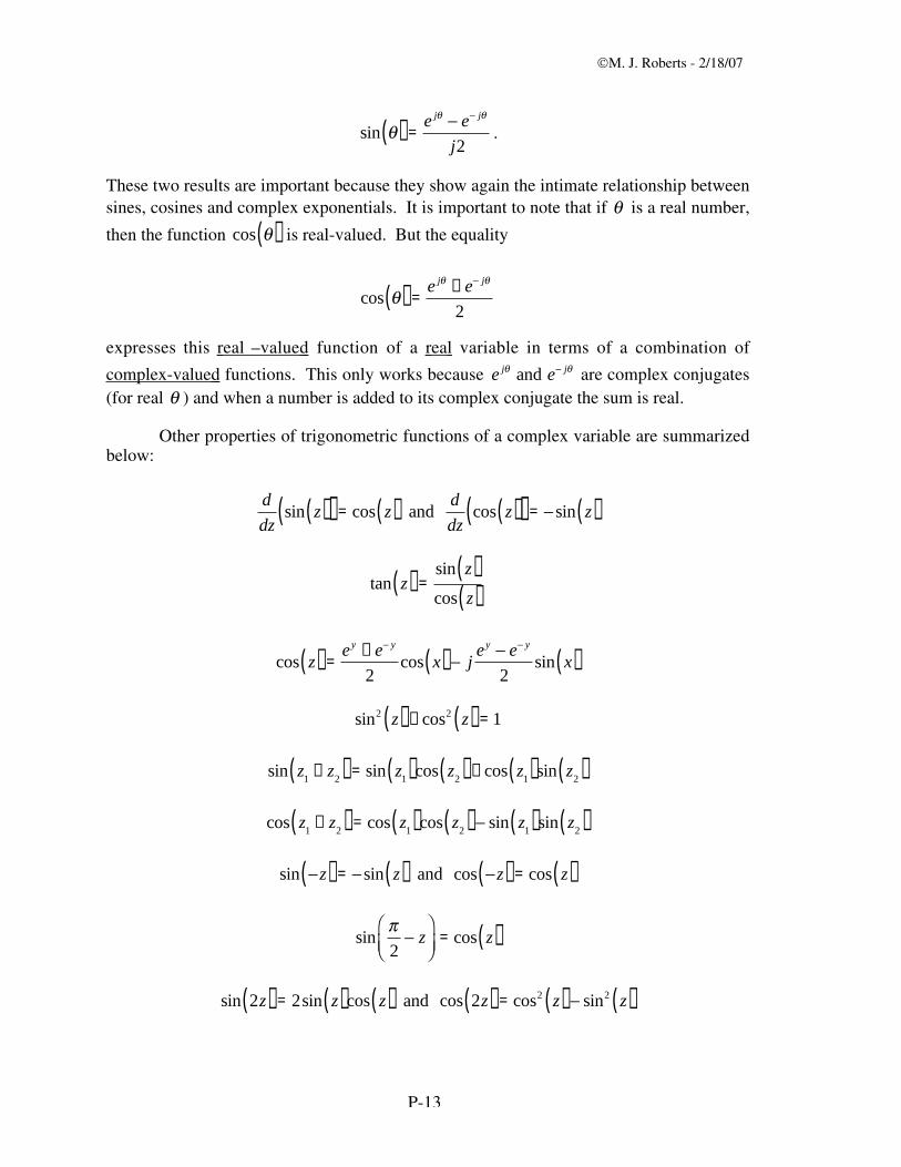
sin( ) =e
je
j
j2.
These two results are important because they show again the intimate relationship betweensines, cosines and complex exponentials. It is important to note that if is a real number,
then the function cos( ) is real-valued. But the equality
cos( ) =
ej
+ ej
2
expresses this real –valued function of a real variable in terms of a combination of
complex-valued functions. This only works because e
jand e
j are complex conjugates(for real ) and when a number is added to its complex conjugate the sum is real.
Other properties of trigonometric functions of a complex variable are summarizedbelow:
d
dzsin z( )( ) = cos z( ) and
d
dzcos z( )( ) = sin z( )
tan z( ) =sin z( )cos z( )
cos z( ) =
ey
+ ey
2cos x( ) j
ey
ey
2sin x( )
sin
2z( ) + cos
2z( ) = 1
sin z
1+ z
2( ) = sin z
1( )cos z
2( ) + cos z
1( )sin z
2( )
cos z
1+ z
2( ) = cos z
1( )cos z
2( ) sin z
1( )sin z
2( )
sin z( ) = sin z( ) and cos z( ) = cos z( )
sin2
z = cos z( )
sin 2z( ) = 2sin z( )cos z( ) and cos 2z( ) = cos
2z( ) sin
2z( )

M. J. Roberts - 2/18/07
P-14
MATLAB implements all the exponential and trigonometric functions. Theexponential function is exp, the sine function is sin, the cosine function is cos, the tangentfunction is tan, etc... In the trigonometric functions, the argument is always interpreted asan angle in radians. For example,
»exp(1)
ans =
2.7183
»exp(-j*pi)
ans =
-1
»cos(3*pi/4)
ans =
-0.7071
»tan(-pi/4)
ans =
-1.0000
P.4 Complex Functions of a Real Variable
In transform analysis there are many examples of complex functions of a realvariable. Since the function value is complex, it cannot be as simply graphed as a singleplot of a real function of a real variable. There are several methods of plotting functionslike this and each has its advantages and disadvantages. We can plot the real andimaginary parts separately as functions of the real independent variable or plot themagnitude and phase separately as functions of the real independent variable or plot thereal and imaginary parts versus the independent variable in one three-dimensionalisometric plot. As an illustrative example, suppose we want to plot the function
x t( ) = e
j2 t . Figure P-7 through Figure P-9 illustrate the three types of plots of this
function.

M. J. Roberts - 2/18/07
P-15
t2
Re(x(t))
-1
1
t2
Im(x(t))
-1
1
Figure P-7 Real and imaginary parts plotted separately versus the independent variable
t2
|x(t)|
1
t2
Phase of x(t)
-π
π
Figure P-8 Magnitude and phase plotted separately versus the independent variable
t2
1
Re(x( t ))1
Im(x( t ))
1
-1
-1
Figure P-9 Real and imaginary parts plotted together versus the independent variable in athree-dimensional isometric plot
Although plots of the real and imaginary parts are sometimes useful, for mostanalysis purposes, separate plots of the magnitude and phase of a complex function of areal variable are preferred. In the study of transform methods, the independent variablewill often be frequency f or instead of time t.
Consider a complex function of radian frequency

M. J. Roberts - 2/18/07
P-16
H j( ) =1
1+ j.
How would we plot its magnitude and phase? The square of the magnitude of anycomplex number is the product of the number and its complex conjugate. Therefore the
magnitude of H j( ) is
j( ) = j( ) *
j( ) . In this case
j( ) =1
1+ j
1
1 j=
1
1+2
=1
1+2
.
The phase of a complex number is the inverse tangent of the ratio of its imaginary part to
its real part. The real and imaginary parts of H j( ) are
Re H j( )( ) = Re1
1+ j
1 j
1 j= Re
1 j
1+2
=1
1+2
and
Im H j( )( ) = Im1
1+ j
1 j
1 j= Im
1 j
1+2
=j
1+2
.
Therefore the phase of H j( ) is
H j( ) = tan1
Im H j( )( )Re H j( )( )
= tan1
j
1+2
1
1+2
= tan1
j( ) .
It should be noted here that the inverse tangent function is multiple-valued . This means
that, strictly speaking, there is a countable infinity of correct values of
H j( ) at any
arbitrary value of . (There is also an uncountable infinity of incorrect values!) If is
any correct value of
H j( ) , then + 2n , n any integer, is also a correct value of
because the sines of and + 2n are identical and the cosines of and + 2n are
identical and therefore the real part of H j( )
H j( ) cos + 2n( ) is the same for any
integer value of n and the imaginary part of H j( )
H j( ) sin + 2n( ) is also the same
for any integer value of n. To avoid any needless confusion caused by the multiple-valuednature of the inverse tangent function it is conventional to restrict plots of phase to lie insome range of angles for which the inverse tangent function is single-valued, for example,
< . This simply means that when we evaluate the inverse tangent function wechoose a correct value that lies in that range. Since any correct phase is as good as any

M. J. Roberts - 2/18/07
P-17
other this causes no problems. Using this convention, the magnitude and phase of H j( )
versus frequency are illustrated in Figure P-10.
ω-10 10
|H(jω)|
1
ω-10 10
H(jω)π2
π2
-
Figure P-10 Magnitude and phase of
H j( ) =1
1+ j
These plots were made using MATLAB so they would be very accurate. But it isimportant to develop quick approximate methods to visualize and sketch the magnitudeand phase of complex functions of a real variable. This is a skill that helps an engineer inthe design and analysis of systems. Look again at the function
H j( ) =1
1+ j.
We can get a very good quick indication of the general shape of the magnitude and phaseby finding the magnitude and phase at some extreme points, approaching zero fromabove or below and approaching plus or minus infinity.
For equal to zero, the denominator 1+ j of
H j( ) is simply 1 and
H j( )
obviously equals one, the real number one whose magnitude is one and whose phase is
zero. For approaching zero from above (from positive values) the phase of H j( ) is
the phase of the numerator (which is zero) minus the phase of the denominator. The phaseof the denominator for small positive is a small positive phase. Therefore the phase of
H j( ) is zero minus a small positive phase, that is, a small negative phase. This shows
that as approaches zero from above the phase is negative and approaching zero. Bysimilar reasoning as approaches zero from below (from negative values), the phase ispositive and approaching zero. This analysis is confirmed by the phase plot in FigureP-10.

M. J. Roberts - 2/18/07
P-18
As approaches positive infinity, the denominator 1+ j becomes infinite in
magnitude and, since the numerator is finite, the magnitude of H j( ) approaches zero.
Also the 1 in the denominator 1+ j of
H j( ) becomes negligible in comparison with
j and the phase of H j( ) approaches zero minus / 2 which is / 2 radians. As
approaches negative infinity, the phase of H j( ) approaches zero minus / 2 which is
/ 2 radians. These limits are also confirmed by Figure P-10. For a function as simple
as this example, we can sketch a fairly accurate magnitu 1 f 2
+ jf de and phase plot veryquickly just using these simple principles.
Now let’s try a somewhat more complicated example, a complex function of cyclicfrequency f
H f( ) =1 f 2
1 f 2+ jf
.
Using the quick-approximation ideas just presented, at f = 0
H f( ) is 1. For f
approaching zero from above, the phase is the phase of 1 f 2 , which for small f is zero,
minus the phase of 1 f 2
+ jf , which for small positive f is a small positive phase.Therefore the phase for f approaching zero from above is a small negative phaseapproaching zero. Similarly for f approaching zero from below the phase is a smallpositive phase approaching zero.
For f approaching either positive or negative infinity, the f
2 terms in the
numerator 1 f 2 and in the denominator dominate and the ratio of numerator to
denominator approaches
f 2( ) / f 2( ) which is one. So the magnitude approaches one
and the phase approaches zero in that limit. So far we see that for very small or very largevalues of f, the magnitude approaches one and the phase approaches zero. We might beinclined to assume that the magnitude is one for all frequencies. But consider the case
f = ±1. At those values of f, the magnitude of H f( ) is zero. Therefore the magnitude
must begin at one for f = 0 , go to zero at
f = ±1 and approach one for f approaching± . Also, as f approaches +1 from below, the numerator is a small positive real numberwith a phase of zero, and the denominator is a small positive number plus an imaginarynumber approaching j. The denominator phase is approaching / 2 so the phase of
H f( ) is approaching / 2 . As f approaches zero from above, the numerator is a small
negative real number with a phase of , the phase of the denominator approaches / 2
and the phase of H f( ) approaches / 2 . So as f moves from just below +1 to just above
+1, the phase changes discontinuously from / 2 to / 2 . Notice that thisdiscontinuity in the phase occurs where the magnitude is exactly zero. Figure P-11 is a

M. J. Roberts - 2/18/07
P-19
plot generated by MATLAB of the magnitude and phase of H f( ) and it confirms all
these observations about the magnitude and phase.
-8 -1 81
-1 1-8 8
1
f
f
π2
π2
1 - f 2
1 - f + jf 2
1 - f 2
1 - f + jf 2
Figure P-11 Magnitude and phase of a complex function of a real frequency
We have already explored the multiple-valued nature of the inverse tangent function.There is one more wrinkle in the computation of phase that is important. We willillustrate it by finding the phase of the complex number
z = 1+ j . If we take a simpledirect approach using a hand-held calculator we might calculate the phase as
Phase of z = tan1
1
1= tan
11( ) =
4.
However a plot of z in the complex plane (Figure P-12) shows that this answer is wrong.

M. J. Roberts - 2/18/07
P-20
x
y
z1
-1
θ
Figure P-12 Location of 1+ j in the complex plane
The plot shows that z lies in the second quadrant. The calculator result indicates that z liesin the fourth quadrant. Instead of simply evaluating the inverse tangent of a complexnumber or function we should evaluate the four-quadrant inverse tangent using ourknowledge of the real and imaginary parts separately instead of knowledge of their ratioalone. This enables us to locate the quadrant in which the number lies and eliminate afalse answer which lies at radians from the correct answer in the diagonally-oppositequadrant. The problem in using the simple inverse tangent function without thinking isthat
1+ j( ) = tan1
1
1= tan
11( ) =
4
and
1 j( ) = tan1
1
1= tan
11( ) =
4.
A hand-held calculator typically returns a value using the inverse tangent function, inthe range / 2 < / 2 . The exact location of the complex number in the complexplane is lost when the ratio of the imaginary to real part is taken. Therefore any four-quadrant inverse tangent must take two arguments, the real and imaginary parts separately,rather than their ratio. (MATLAB has a function angle which finds the four-quadrantangle or phase of a complex number.) Using a four-quadrant inverse tangent, the correctanswer in this example would be
1+ j( ) = tan1
1
1=
3
4.
What is the phase of the real number -1? Using the four quadrant tangent, theanswer is (plus or minus any integer multiple of 2 ). Therefore when plotting themagnitude and phase of a real-valued function the magnitude is always non-negative andthe phase switches back and forth between zero and (or ) as the function values gothrough zero. Of course, plotting the magnitude and phase of a real function is a little silly

M. J. Roberts - 2/18/07
P-21
since it can be plotted with positive and negative values on a single plot. But, asillustrated above, as soon as the function becomes complex, magnitude and phase plots areone of the best ways to graphically represent the function.________________________________________________________________________
Example P-3 Magnitude and phase of a complex function of a real variable
Using MATLAB, plot the magnitude and phase of the function,
X f( ) =1 f 2
1 f 2+ jf
versus f, which appears in Figure P-11.
This function can be easily plotted using the fplot command in MATLAB. Thefollowing sequence of MATLAB commands produces the plot of the magnitude and phaseof this function in Figure P-13.
subplot(2,1,1) ; fplot('abs((1-f^2)/(1-f^2+j*f))',[-8,8],'k') ;
xlabel('Frequency, f (Hz)') ; ylabel('|X(f)|') ;
subplot(2,1,2) ; fplot('angle((1-f^2)/(1-f^2+j*f))',[-8,8],'k') ;
xlabel('Frequency, f (Hz)') ; ylabel('Phase of X(f)') ;
-8 -6 -4 -2 0 2 4 6 80
0.2
0.4
0.6
0.8
1
Frequency, f (Hz)
|X(f
)|
-8 -6 -4 -2 0 2 4 6 8-2
-1
0
1
2
Frequency, f (Hz)
Pha
se o
f X(f
)
Figure P-13 Magnitude and phase of
X f( ) =1 f 2
1 f 2+ jf
Although this plot is easy to generate it does not allow as much user control overformatting and scaling as a somewhat more involved plotting technique. We are plotting acontinuous function of the variable f. MATLAB does not know what a “continuous”function is. MATLAB can only draw straight lines. Therefore we must formulate theproblem so as to get a plot that looks like the continuous function using numericalcalculations and plotting with straight lines (Figure P-14).

M. J. Roberts - 2/18/07
P-22
Actual Function
What MATLAB Draws
Functional ValuesComputed by MATLAB
t
g(t)
Figure P-14 Illustration of how MATLAB plots an approximation to a function
When we use fplot MATLAB decides how to assign the values of the independentvariable at which the function values will be calculated. Although the algorithm used byMATLAB is generally very good we can have more control over the plotting of thefunction and formatting of the plot if we generate the independent variable valuesourselves and use the plot command instead. The plot command is more primitive thanthe fplot command but it also allows the programmer more options in plotting.
In order to get a smooth looking curve we must be sure that the points in f are closeenough together that when we draw straight lines between points the result looks like the
actual curved contours of X f( ) . The plot in Figure P-11 covers the range
8 < f < 8 .How many points do we need to make the plot look smooth? The main requirement onhow close the points should be is to resolve the region around
f = ±1 where there aresome sharp corners in the function’s magnitude and phase. Let’s try a spacing betweenpoints of 1 / 10 . The MATLAB program then might look like the following code.
% Program to plot the function, (1-f^2)/(1-f^2+j*f)
%-----------------------------------------------------------------
% This section actually calculates values of the function
%-----------------------------------------------------------------
df = 1/10 ; % "df" - spacing between frequencies
fmin = -8 ; fmax = 8 ; % "fmin" & "fmax" - beginning and ending
% frequencies
f = fmin:df:fmax ; % "f" - vector of frequencies for
% plotting function with straight lines
% between points
X = (1-f.^2)./(1-f.^2+j*f) ; % "X" - vector of function values
%-----------------------------------------------------------------
% This section displays the results and formats the plots
%-----------------------------------------------------------------
subplot(2,1,1) ; % Plot two plots, one on top and one on
% the bottom.
% First draw the top plot.
p = plot(f,abs(X),'k') ; % Plot |X(f)| with black lines between
% points

M. J. Roberts - 2/18/07
P-23
set(p,'LineWidth',2) ; % Make the plot line heavier
xlabel('Frequency, f (Hz)') ; % Label the "f" axis
ylabel('|X(f)|') ; % Label the "|X(f)|" axis
title('Plot of (1-f.^2)./(1-f.^2+j*f)') ; % Title the plots
subplot(2,1,2) ; % Draw the second plot.
p = plot(f,angle(X),'k') ; % Plot the phase (angle) of X(f) with
% black lines between points
set(p,'LineWidth',2) ; % Make the plot line heavier
xlabel('Frequency, f (Hz)') ; % Label the "f" axis
ylabel('Phase of X(f)') ; % Label the "Phase of X(f)" axis
The actual MATLAB graph is displayed in Figure P-15.
-8 -6 -4 -2 0 2 4 6 80
0.2
0.4
0.6
0.8
1
Frequency, f (Hz)
|X(f
)|
Plot of (1-f. 2)./(1-f. 2+j*f)
-8 -6 -4 -2 0 2 4 6 8-2
-1
0
1
2
Frequency, f (Hz)
Pha
se o
f X(f
)
Figure P-15 MATLAB plots of the magnitude and phase of
X f( ) =1 f 2
1 f 2+ jf
Although this plot looks very much like Figure P-11, it is not exactly the same. The jumpsin the phase plot are not as nearly vertical as in Figure P-11. That is because the spacingbetween points is not quite small enough. Figure P-16 is the phase plot, redone with thepoint locations indicated by small dots.
-8 -6 -4 -2 0 2 4 6 8-2
-1
0
1
2
Frequency, f (Hz)
Pha
se o
f X(f
)
Figure P-16 MATLAB plot of the phase emphasizing the points at which phase is actuallycalculated
Try a smaller spacing and see what your plot looks like. (This is our first consideration of

M. J. Roberts - 2/18/07
P-24
the sampling problem of representing a continuous function by discrete samples.)
Why is there a jump in the phase anyway? Does the phase of X f( ) really change
discontinuously at f = ±1? Notice that the size of the jump is exactly radians. One way
to grasp what is really happening near f = ±1 is to graph the imaginary part of
X f( )
versus the real part of X f( ) in the complex plane, for a succession of f’’s near
f = 1
(Figure P-17).
Re(X(f))
Im(X(f))
f = 0.9
f = 0.95
f = 1
f = 1.05
f = 1.1
Figure P-17 Plot of the imaginary part of X f( ) versus the real part of
X f( )
At f = 1 , the plot goes through the origin of the complex plane, tangent to the imaginary
axis. Therefore the angle of a vector from the origin to the complex value of X f( )
approaches / 2 just before reaching the origin and as it passes through the origin theangle changes suddenly to + / 2 , agreeing with the plot in Figure P-15. So the phase is
discontinuous , even though the complex value of X f( ) is continuous ! This can only
happen where the complex value of X f( ) passes through zero. At any other point in the
complex plane a phase discontinuity would cause a discontinuity in the complex value of
X f( ) . ( Unless the size of the discontinuity of phase is exactly an integer multiple of 2
radians. In the case in which the discontinuity of phase is exactly an integer multiple of2 radians the phase discontinuity is only apparent, not real, because we can alwaysreplace that phase with one which is continuous, making the phase plot again continuous.)________________________________________________________________________

M. J. Roberts - 2/18/07
P-25
Exercises
(On each exercise, the answers listed are in random order.)
1. Find all the solutions of
(a) z2
+ 8 = 2 (b) z2
2z + 10 = 0 (c) 7z2
+ 3z + 8 = 5
Answers: 0.2143 ± j0.6186
± j 6 1± j3
2. If z
1= 3 j6 and
z
2= 2 + j8 and z = x + jy , find x and y in each case.
(a) z = z
1+ z
2(b)
z = z
1z
2(c)
z = z
2z
1
(d) z = z
1z
2(e)
z =z
1
z2
(f)
z =z
2
z1
(g)
z =1
z1
(h)
z =1
z2
Answers:
1
34j
2
17 1+ j14
1
15+ j
2
15 5 + j2
54 + j12
14
15+ j
4
5 1 j14
21
34j
9
17
3. If z
1=
1+ j2
5 and
z
2= j 4 j3( ) and z = x + jy , find x and y in each case.
(a) z = z
1+ z
2(b)
z = z
1
*+ z
2(c)
z = z
2
*
(d) z = z
2+ z
2
* (e) z = z
2z
2
* (f) z = z
1z
1
*
(g)
z =z
1
z2
*
Answers:
16
5+ j
18
5 3 j4
1
5 6
16
5+ j
22
5 j8
1
25+ j
2
25

M. J. Roberts - 2/18/07
P-26
4. If z
1= j 3( )
*
and
z2
=3 j2
4 j find
z in each case.
(a) z = z
1(b)
z = z
2(c)
z = z
1z
1
*
(d) z = z
2z
2
* (e) z = z
1+ z
2
* (f) z = z
2z
1
*
(g)
z =z
1+ z
2
z1
(h)
z =z
1
z1
*(i)
z =z
2
z2
*
Answers:
4505
171
13
1710 1
130
17 10
3757
17 10
13
17
5. Find the magnitude and angle of these complex numbers.
(a) z = 1+ j (b)
z = 1 j (c) z = 3 j3
(d) z = 4 + j3 (e)
z = 1+ j( ) 1 j( ) (f)
z =1
1+ j
(g)
z =2 j
1+ j3 (h)
z =2 j
1+ j3
*
Answers:
24
± 2n
1
2 4 5 2.498
1
2
1.713
22
1
2
1.713
24
± 2n
3 24
± 2n
6. Find all the distinct solutions to these equations.
(a) z
2= j (b)
z3
= j (c) z5
= 1
(d) z
43 = j (e) z
38 = 0

M. J. Roberts - 2/18/07
P-27
Answers:
14
or13
4
16
or 15
6or 1
2
2 0 or 22
3or 2
2
3
15
or 13
5or 1 or 1
5or 1
3
5
1.333 0.0804 or 1.333 1.651 or 1.333 3.061 or 1.333 1.490
7. Evaluate these exponential functions.
(a) ej (b) e
j / 2 (c) ej / 2 (d) e
j3 / 2
(e) ej
+ ej (f)
e
j / 2+ e
j / 2( )*
(g) e + e
(h) e
/ 2+ e
/ 2( )*
Answers: 9.621, j, -2, -j, 23.184, 0, -1, -j
8. If z = x + jy = Aej , find x, y, A and .
(a) z = 4ej / 2 (b) z = 4e
1 j / 2 (c) z = 4e
1 j / 2( ) j2e1 j / 2( )
(d) z = 10e
j3 / 2( )3
(e) z = e
j3 / 2( )3/ 2
Answers:
x = 0 , y = 4 , A = 4 , =
2+ 2n
x = 0 , y = 1000 , A = 1000 , =
2+ 2n
x = 0 , y = 8 , A = 8 , =
2+ 2n
x =1
2, y =
1
2, A = 1 , =
4+ 2n
or
x =1
2, y =
1
2, A = 1 , =
5
4+ 2n
x = 0 , y = 10.87 , A = 10.87 , =
2+ 2n
9. Using MATLAB plot the magnitude and phase of the following complex functionsof the real independent variable t, f or over the range indicated.

M. J. Roberts - 2/18/07
P-28
(a) x t( ) = 2e
j4 t, 1 < t < 1
(b) x t( ) = 2e
1+ j4( )t, 4 < t < 4
(c)
X f( ) =1
1+ j2 f, 2 < f < 2
(d)
X j( ) =j
1+ j, 4 < < 4
Answers:
t-4 4
|x(t)|
109.1963
t-4 4
x(t)
-≠
≠
ω-4 π 4π
|X(jω)|
1
ω-4 π 4π
X(jω)
- ≠
≠

M. J. Roberts - 2/18/07
P-29
f -2 2
|X( f )|
1
f -2 2
X( f )
-π
π
t-1 1
|x(t)|2
t-1 1
x(t)
-π
π
10. Convert these complex numbers to the polar form Aej with an angle in the
range, < .
(a) 1+ j (b)
3 j2 (c) j (d) j + 1
11. Convert these complex numbers to the rectangular form x + jy .
(a) ej (b) 4 45° (c) 3e
2 j4 (d)
10ej11
4
12. Find the numerical value of z in both the rectangular and polar forms.
(a) z = 2e
1+ j / 2+ 4 j2 (b)
z = 1 j( ) 4 + j5( )
2
(c) z = j( )
3
(d)
z =2e
j
1+ j( )4
(e)
z =2e
j
1 j( )4
(f) z = e1+ j
e1 j
13. Using MATLAB, plot graphs of the magnitude and phase of the followingfunctions of the real variable f over the range indicated.
(a)
X f( ) =10
1+ jf
100
, 400 < f < 400

M. J. Roberts - 2/18/07
P-30
(b)
X f( ) =j10 f
1+ jf
100
, 400 < f < 400
(c) X f( ) = e j f e j2 f
, 8 < f < 8
(d)
X f( ) =5
1 f 2+ j
f
4
, 4 < f < 4
(e)
X j( ) =1
j ej3 / 4( ) j e
j5 / 4( ) j ej3 / 4( ) j e
j5 / 4( ), 2 < < 2
(f)
X j( ) =j( )
4
j ej3 / 4( ) j e
j5 / 4( ) j ej3 / 4( ) j e
j5 / 4( ), 2 < < 2
14. (a) Show that the magnitude of the complex function ejx , x a real number, is
one, regardless of the value of x.
(b) Find the simplest expression you can for the phase of ejx as a function of x.
(c) Graph the phase of ejx by hand and then write a MATLAB program to
graph the same phase. The graphs should extend over values of x in therange, 4 < x < 4 . If the graphs are different, explain why.