Embed Size (px)
Citation preview
Weather Forecasting &
Business Management
Systems
Tools for Better Business Management
A report for
By Robin Schaefer
2012 Nuffield Scholar
October 2014
Nuffield Australia Project No 1219
Sponsored by:
2
© 2010 Nuffield Australia.
All rights reserved.
This publication has been prepared in good faith on the basis of information available at the date of publication without any independent verification. Nuffield Australia does not guarantee or warrant the accuracy, reliability, completeness or currency of the information in this publication nor its usefulness in achieving any purpose.
Readers are responsible for assessing the relevance and accuracy of the content of this publication. Nuffield Australia will not be liable for any loss, damage, cost or expense incurred or arising by reason of any person using or relying on the information in this publication.
Products may be identified by proprietary or trade names to help readers identify particular types of products but this is not, and is not intended to be, an endorsement or recommendation of any product or manufacturer referred to. Other products may perform as well or better than those specifically referred to.
This publication is copyright. However, Nuffield Australia encourages wide dissemination of its research, providing the organisation is clearly acknowledged. For any enquiries concerning reproduction or acknowledgement contact the Publications Manager on ph: (03) 54800755.
Scholar Contact Details
(Name)
Organisation
(Address)
Phone:
Fax:
Email:
Robin Schaefer
Bulla Burra Operations
PO Box 182 Loxton SA 5333
(08) 85846350
(08) 85846350
In submitting this report, the Scholar has agreed to Nuffield Australia publishing this material in its edited form.
Nuffield Australia Contact Details
Nuffield Australia Telephone: (03) 54800755
Facsimile: (03) 54800233
Mobile: 0412696076
Email: [email protected]
PO Box 586 Moama NSW 2731
3
Executive Summary
Successfully managing a farm business has never been so complex, so risky and required such
a diverse set of skills. Yet many businesses today are managing and even thriving in this
climate. What sets them apart from other businesses which are struggling? There are probably
many reasons for this but management skills, a good understanding of their risks, and putting
systems in place to manage these risks would be part of the answer.
Better day to day and long term farm business decisions can be made with a greater
understanding of the weather and climate risks, and the chance of those conditions occurring.
Understanding weather cycles and weather forecasting and using decision support tools all
adds to a manager’s tool kit. This helps to make sure when a decision is made, the odds are
highest that it is the right decision.
Accuracy in weather forecasting has improved significantly in the last thirty years.
Benchmarking data shows accuracy for the best three day weather forecast has improved by
27 percent, and is now 97 percent accurate. The best five day forecast has improved by 45
percent and is now 90 percent accurate and the best seven day forecast has improved by 45
percent, it is now 78 percent accurate. There was no ten day forecast 30 years ago, but this
now has an accuracy of 48%.There are many factors that have a longer term influence on our
weather; as these are better understood and computing power increases, accuracy continues to
improve.
The improvements in forecasting accuracy mean that weather forecasts can now be a more
effective tool in a farm manager’s tool kit. Managers need to understand that a forecast will
never be 100% accurate. The critical point is that they must be used to manage risk, not create
more risk. A good understanding of how the forecasts are produced can significantly affect
their usefulness and the management of risk.
Private weather forecasters tend to be at the cutting edge of developing new methods in
seasonal forecasting; they tend to take more risks. Although some of their methods are not
recognised by the institutional forecasting community, they certainly show where more
research can be targeted. Private forecasters tend to have closer links to the agricultural
community and so are able to produce forecasts more suited to farmers’ requirements.

4
Foreword
Meteorologists I visited agreed that “to their knowledge a project like this had never been
undertaken before.”
This has made the project both exciting and daunting.
Receiving a Nuffield Australia Farming Scholarship provided me with an amazing
opportunity to gain a perspective of agriculture that only relatively few farmers will ever
have. It has introduced me to a network of inspirational and motivated people and challenged
me to think beyond our farming business, beyond our town, beyond our region and beyond
Australia. It has been far more than just a research project; it has helped me to grow as a
husband, father, businessman and member of our community.
In the past 11 years our farming business has grown from cropping 1,000 ha to cropping 9,000
ha. The expanded capital investment now required to manage our business has increased our
risk profile. The business is more complex and requires different management skills. During
this time we have experienced eight years that have been in the lowest 30 percent of growing
season rainfall in one hundred years of records. Five have been in the lowest 20 percent.
The combination of these factors has increased my interest in the weather and in business
management systems and led me to undertake a Nuffield Australia Farming Scholarship.
The weather is an essential part of planning daily operations and in the longer term can mean
the difference between a profitable and unprofitable year. As a farmer I am also a weather
forecaster, I refer to as much information as possible, from as many sources as I have
available, then use this information to influence my decision making. The information may be
gleaned from a website, an application (app.) on my mobile phone, the television, a
subscription-based service, or by observing nature and my environment. How much weight I
place on each piece of information, when making decisions, is based on my perception of the
reliability of the information.

5
I use management systems to help with decision making and simplify staff management. They
can provide a way of drawing information together to guide our staff and business to achieve
the best outcome. They simplify processes.
As a result of undertaking the Nuffield Australia Farming Scholarship, I have increased my
knowledge of weather forecasting and now have a better understanding of what goes on
behind the forecast. I have learnt how much the science of weather forecasting has improved
and understand why it is so complex. This helps me to make better use of the information
received in a forecast. I can also see areas where more research is needed.
I have been able to draw on management systems used by farmers and meteorologists in
Australia and around the world. These will improve the practical and business management of
our farming enterprise and others around Australia.
6
Acknowledgements
I am sincerely grateful to the many people who have supported me, and enabled me to share
the knowledge I have gained with you, especially to the GRDC for funding my scholarship.
Without their sponsorship my scholarship and project would not have been possible. Thank
you to my friends and colleagues in the Nuffield Alumni who helped to organise the
Contemporary Scholars Conference and the Global Focus programme. Also the businesses
and organisations who opened their doors to us, answering our many questions. Thank you to
all my fellow 2012 Nuffield Australia Farming Scholarship recipients for sharing the journey.
I would like to specifically thank the following people and organisations who personally gave
up time to help me with my research project.
Manfred Kloepel and staff at European Centre for Medium Range Weather
Forecasting (ECMWF) in England
Ken Mylne, UK Met. Office, England
Jim Bacon, Weatherquest, England
Simon Ward, Increment Ltd., England
Ray Garnett of Agro Economic Consulting, Canada
Hope Pjesky, an Eisenhower Fellow, USA
Chuck Coffey and staff at The Samuel Roberts Noble Foundation, USA
Al Sutherland and staff at The National Weather Centre, USA
Jesus Fernandez, National Institute of Agricultural Technology (INTA) Research
Centre, Argentina
Ken Ring, Predict Weather, New Zealand

7
There were many more people who also helped with researching my project but are too
numerous to mention; thank you to you all. To Emma Leonard for editorial work in helping to
improve my report; a big thank you for the time you put in.
Thank you to my business partner and fellow Nuffield scholar John Gladigau for encouraging
me to apply to Nuffield, for helping to set up our business ‘Bulla Burra’ and to make it
possible for my 17 weeks absence. Thank you also to our employees for taking on extra
responsibility in my absence and to you all for supporting Rebecca and my family.
Finally I would like to thank my wife Rebecca for her support and dedication, and also my
children Brianna, Jordan, Caleb, Isaac and Elise. They all took on extra responsibilities and
personally grew through my absence. Words cannot express my sincere thanks to you all.
8
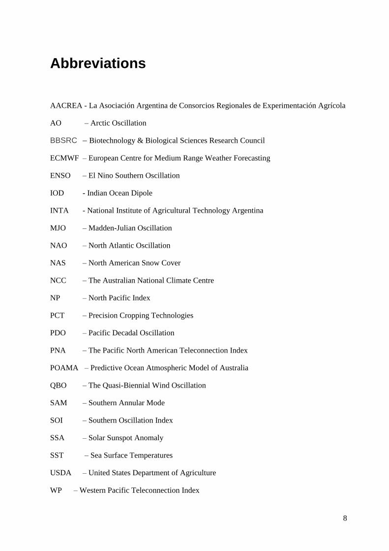
Abbreviations
AACREA - La Asociación Argentina de Consorcios Regionales de Experimentación Agrícola
AO – Arctic Oscillation
BBSRC – Biotechnology & Biological Sciences Research Council
ECMWF – European Centre for Medium Range Weather Forecasting
ENSO – El Nino Southern Oscillation
IOD - Indian Ocean Dipole
INTA - National Institute of Agricultural Technology Argentina
MJO – Madden-Julian Oscillation
NAO – North Atlantic Oscillation
NAS – North American Snow Cover
NCC – The Australian National Climate Centre
NP – North Pacific Index
PCT – Precision Cropping Technologies
PDO – Pacific Decadal Oscillation
PNA – The Pacific North American Teleconnection Index
POAMA – Predictive Ocean Atmospheric Model of Australia
QBO – The Quasi-Biennial Wind Oscillation
SAM – Southern Annular Mode
SOI – Southern Oscillation Index
SSA – Solar Sunspot Anomaly
SST – Sea Surface Temperatures
USDA – United States Department of Agriculture
WP – Western Pacific Teleconnection Index
9
Contents
Executive Summary ................................................................................................................. 3
Foreword ................................................................................................................................... 4
Acknowledgements ................................................................................................................... 6
Abbreviations ............................................................................................................................ 8
Objectives ................................................................................................................................ 14
Chapter 1: Introduction ......................................................................................................... 15
Chapter 2: Key Developments In Weather Forecasting ..................................................... 17
A Meteorological Timeline ................................................................................................... 17
Meteorological Records ........................................................................................................ 19
Meteorology for defence, aviation and society ..................................................................... 19
Teleconnections .................................................................................................................... 20
Teleconnections affecting Australia (and other surrounding countries) ........................... 21
Other Significant Teleconnections (See Appendix 2) ....................................................... 21
Forcing .................................................................................................................................. 21
Astrometeorology ................................................................................................................. 22
Chapter 3: Weather Forecasting Methods ........................................................................... 23
European Centre for Medium Range Weather Forecasting (ECMWF) ............................... 23
Deterministic forecasts; ..................................................................................................... 25
Ensemble forecasts ............................................................................................................ 26
Agro Climatic Consulting ..................................................................................................... 28
Weatherquest ........................................................................................................................ 30
Oklahoma Mesonet ............................................................................................................... 33
Predict Weather .................................................................................................................... 35
Holton Weather ..................................................................................................................... 36
Chapter 4: The Progression of Weather Forecasting ......................................................... 38

10
Short term forecasting ........................................................................................................... 38
Medium term forecasts (See Appendix 2.) ......................................................................... 39
Long term forecasts (See Appendix 2.) .............................................................................. 40
Chapter 5: Micrometeorology ............................................................................................... 41
A New Science ..................................................................................................................... 41
Stamina, a Micrometeorology Research Project at the Biotechnology & Biological Sciences
Research Council (BBSRC) Rothamsted ............................................................................. 42
Chapter 6. Natural Climate Variability ............................................................................... 43
Chapter 7:The Future of Weather Forecasting ................................................................... 46
Private Sector versus Public Sector ...................................................................................... 46
New Radar Technologies ...................................................................................................... 46
Dual-polarization technology ............................................................................................ 46
Phased Array Radar .......................................................................................................... 47
Teleconnections .................................................................................................................... 47
Astrometeorology ................................................................................................................. 47
Cycles ................................................................................................................................... 47
Volcanic ................................................................................................................................ 48
Chapter 8: Decision Support Tools and Systems ................................................................ 50
UK Met Office ...................................................................................................................... 50
The Oklahoma Mesonet ........................................................................................................ 52
Australia ................................................................................................................................ 52
Climate Kelpie .................................................................................................................. 52
Australian Rainman ........................................................................................................... 52
Australian Bureau of Meteorology (BOM) ....................................................................... 53
Production Wise ................................................................................................................ 53
Ag Seasons ........................................................................................................................ 53
Graingrowers Monthly Rainfall Forecast Reports ............................................................ 54
11
Weather Related Applications (Apps) .............................................................................. 54
Conclusion ............................................................................................................................... 56
Positioning Your Business .................................................................................................... 56
Managing Without Weather Forecasts ................................................................................. 56
Further Research ................................................................................................................... 57
Recommendations .................................................................................................................. 58
Appendices .............................................................................................................................. 59
1. Traditional Forecasting Tools ....................................................................................... 59
Australian Bush Forecasting Aids ..................................................................................... 59
United States Traditional Weather Forecasting ................................................................ 60
How to Predict the Weather without a forecast ................................................................ 60
Kenya Meteorological Department (KMD) ...................................................................... 60
2. Terms used in this paper ................................................................................................ 61
Short Term Weather Forecasting ...................................................................................... 61
Medium Term Weather Forecasting ................................................................................. 61
Long Term Weather Forecasting ...................................................................................... 61
Teleconnections affecting Australia (and other surrounding countries) ........................... 61
Other Significant Teleconnections .................................................................................... 65
References ............................................................................................................................... 69
Plain English Compendium Summary ................................................................................. 73
Figure 1. Radar sites across Australia, generally located in large cities and towns for aviation,
defence and the general population. (Australian Government Bureau of Meteorology 2013) 20
Figure 2. The ECMWF boardroom (Schaefer 2012) ............................................................... 23
Figure 3. A comparison of accuracy between the main international weather forecasters for
the Southern and Northern hemispheres since 1988. (ECMWF 2012) .................................... 24
Figure 4. Chart showing the improved forecasting skill over time of ECMWF deterministic
forecasts at 80% accuracy for the Northern Hemisphere. (ECMWF 2012) ............................. 26
12
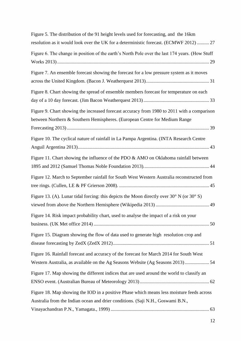
Figure 5. The distribution of the 91 height levels used for forecasting, and the 16km
resolution as it would look over the UK for a deterministic forecast. (ECMWF 2012) .......... 27
Figure 6. The change in position of the earth’s North Pole over the last 174 years. (How Stuff
Works 2013) ............................................................................................................................. 29
Figure 7. An ensemble forecast showing the forecast for a low pressure system as it moves
across the United Kingdom. (Bacon J. Weatherquest 2013). ................................................... 31
Figure 8. Chart showing the spread of ensemble members forecast for temperature on each
day of a 10 day forecast. (Jim Bacon Weatherquest 2013) ...................................................... 33
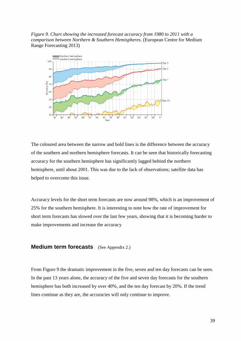
Figure 9. Chart showing the increased forecast accuracy from 1980 to 2011 with a comparison
between Northern & Southern Hemispheres. (European Centre for Medium Range
Forecasting 2013) ..................................................................................................................... 39
Figure 10. The cyclical nature of rainfall in La Pampa Argentina. (INTA Research Centre
Anguil Argentina 2013) ............................................................................................................ 43
Figure 11. Chart showing the influence of the PDO & AMO on Oklahoma rainfall between
1895 and 2012 (Samuel Thomas Noble Foundation 2013). ..................................................... 44
Figure 12. March to September rainfall for South West Western Australia reconstructed from
tree rings. (Cullen, LE & PF Grierson 2008). .......................................................................... 45
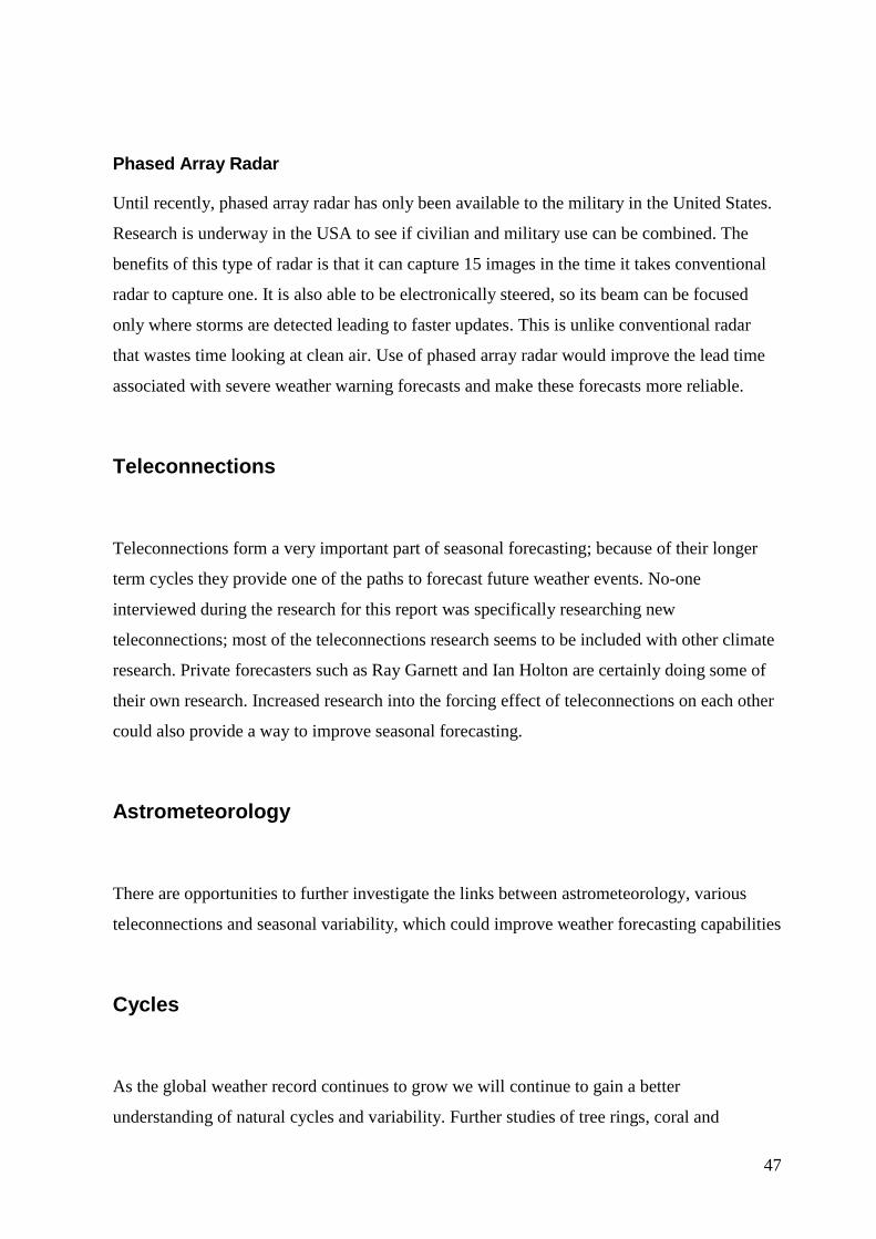
Figure 13. (A). Lunar tidal forcing: this depicts the Moon directly over 30° N (or 30° S)
viewed from above the Northern Hemisphere (Wikipedia 2013) ............................................ 49
Figure 14. Risk impact probability chart, used to analyse the impact of a risk on your
business. (UK Met office 2014) ............................................................................................... 50
Figure 15. Diagram showing the flow of data used to generate high resolution crop and
disease forecasting by ZedX (ZedX 2012) ............................................................................... 51
Figure 16. Rainfall forecast and accuracy of the forecast for March 2014 for South West
Western Australia, as available on the Ag Seasons Website (Ag Seasons 2013) .................... 54
Figure 17. Map showing the different indices that are used around the world to classify an
ENSO event. (Australian Bureau of Meteorology 2013) ......................................................... 62
Figure 18. Map showing the IOD in a positive Phase which means less moisture feeds across
Australia from the Indian ocean and drier conditions. (Saji N.H., Goswami B.N.,
Vinayachandran P.N., Yamagata., 1999) ................................................................................. 63

13
Figure 19. Map showing SAM in a positive phase when westerly winds across Australia
decrease (Wikipedia 2013) ....................................................................................................... 64
Figure 20. Map showing where NP index is calculated ........................................................... 65
Figure 21. Northern Hemisphere map showing the effect on rainfall of a positive and negative
phase of the NAO. (National Earth Science Teachers Association 2010) ............................... 66
Figure 22. World map showing PDO in a positive & negative phase. (Joint Institute for the
Study of Atmosphere and Ocean 2013) ................................................................................... 66
Figure 23. Showing AO in a positive and negative phase (National Snow and Ice Data Centre
2013) Credit J. Walllace University of Washington ............................................................... 67
Figure 24. Position of the Aleutian & Islandic Lows in winter and connection with the
atmospheric bridge. (Japanese Agency for Marine Earth and Science Technology 2003) ...... 68
14
Objectives
The objectives of this research project were to answer the following questions:
1. What weather forecasting methods are used by meteorologists?
2. How reliable are current weather forecasts and is their reliability improving?
3. How can these weather forecasts be used to improve the management of farm
businesses?
4. What is the future for weather forecasting?
5. What tools or systems are available to help make management decisions?
The aim in answering these questions is to increase awareness, understanding and use of
improved methods of weather forecasting and risk management. It will also demonstrate some
of the strengths and weaknesses of the systems to help other farmers select tools that suit their
weather forecasting and risk management needs.

15
Chapter 1: Introduction
Successfully managing a farm business has never been so complex, so risky and required such
a diverse set of skills. Yet many businesses today are managing and even thriving in this
climate. What sets them apart from other businesses which are struggling? There are probably
many reasons for this but management skills, a good understanding of their risks, and putting
systems in place to manage these risks would be part of the answer.
A significant part of risk for broad acre farming businesses relates to weather, the day to
day conditions and climate, the average conditions experienced over a long period of time.
Better day to day and long term farm business decisions can be made with a greater
understanding of the weather and climate risks, and of the chance of those conditions
occurring. Understanding weather cycles and weather forecasting and using decision support
tools all adds to a manager’s tool kit. This helps to make sure that, when a decision is made,
the odds are highest that it is the right decision.
Probably more so than any other occupation, farming is affected by the weather. In day to day
operations decisions are regularly made around the weather. The results of these decisions are
affected by the weather, which in turn can affect the outcomes of the decision.
An example would be when a farmer decides to apply a particular herbicide for weed control.
The herbicide has a rain-fast period of six hours. The farmer has to decide if rain is likely
within that timeframe and which is the greater risk applying today and risking poor control
due to rain destroying the herbicide or waiting for better weather when the weeds will be
larger and harder to kill. If the herbicide is applied its effectiveness is directly affected by the
weather that occurs within the next six hours.
16
The timeframes that farmers regularly make decisions around can be divided into three main
areas.
1. Day to day decisions - usually made for the next 24 to 48 hours;
2. Weekly decisions - planning ahead for the weekly activities; and
3. Seasonal decisions - longer term planning including crop types, area to be cropped,
stocking densities, fertiliser strategy.
Weather forecasting can be divided into the same three time frames and each of these was
addressed in researching this report. To gather the information for answering these three
questions, leading farmers and businesses were interviewed to discover the management
systems helping them to manage their businesses.
Australian Meteorologists indicated that they believed the leading institution in worldwide
weather forecasting is the ECMWF in the United Kingdom. The UK Met Office is also held
in high regard as is the National Weather Centre in Oklahoma, USA. These were the
establishments visited as part of this research project.
Private weather forecasters from countries around the world were harder to find. Early
research led to New Zealand based forecaster Ken Ring and his techniques which warranted
further investigation. The Nuffield network indicated Canadian crop and weather forecaster
Ray Garnett was worth a visit and also encouraged visiting an Argentinean farm management
movement called La Asociación Argentina de Consorcios Regionales de Experimentación
Agrícola (AACREA) to look at the management systems they were using.

17
Chapter 2: Key Developments In Weather
Forecasting
Weather forecasting has always been important to farmers and those closely connected with
the land and sea as their survival and profitability can both be at the mercy of the weather. To
a degree all farmers are meteorologists.
While the term meteorology (the study of atmospheric disturbances or meteors) was invented
by the ancient Greeks in about 300 BC, it was not until the mid 15th
century that the
foundations of today’s systems of weather forecasting were laid.
Despite agriculture’s long association with and reliance on weather forecasting, investment in
meteorological services across the globe have been driven by defence and aviation. The
political profile of climate change and in Australia the Millennium Drought seem to have
helped refocus investments in meteorology, which is offering benefits to agriculture.
A Meteorological Timeline
In ancient civilisations, religious rights and mystery surrounded weather forecasting.
However, drilling down into these practices can sometimes uncover scientific principles at
work in the background. Details of, and links to, weather forecasting tools that have been used
throughout history with varying degrees of success can be found in Appendix 1. Basic
research carried out by independent, Australian weather forecaster Ian Holton, shows that
there appears to be merit behind at least some of these tools.
In the west the modern science of weather observing and recording began in 1654 when an
Italian, Grand Duke Ferdinando II de Medici, sponsored the first weather observing network.
This consisted of nine meteorological stations across Europe. The collected data was sent to
18
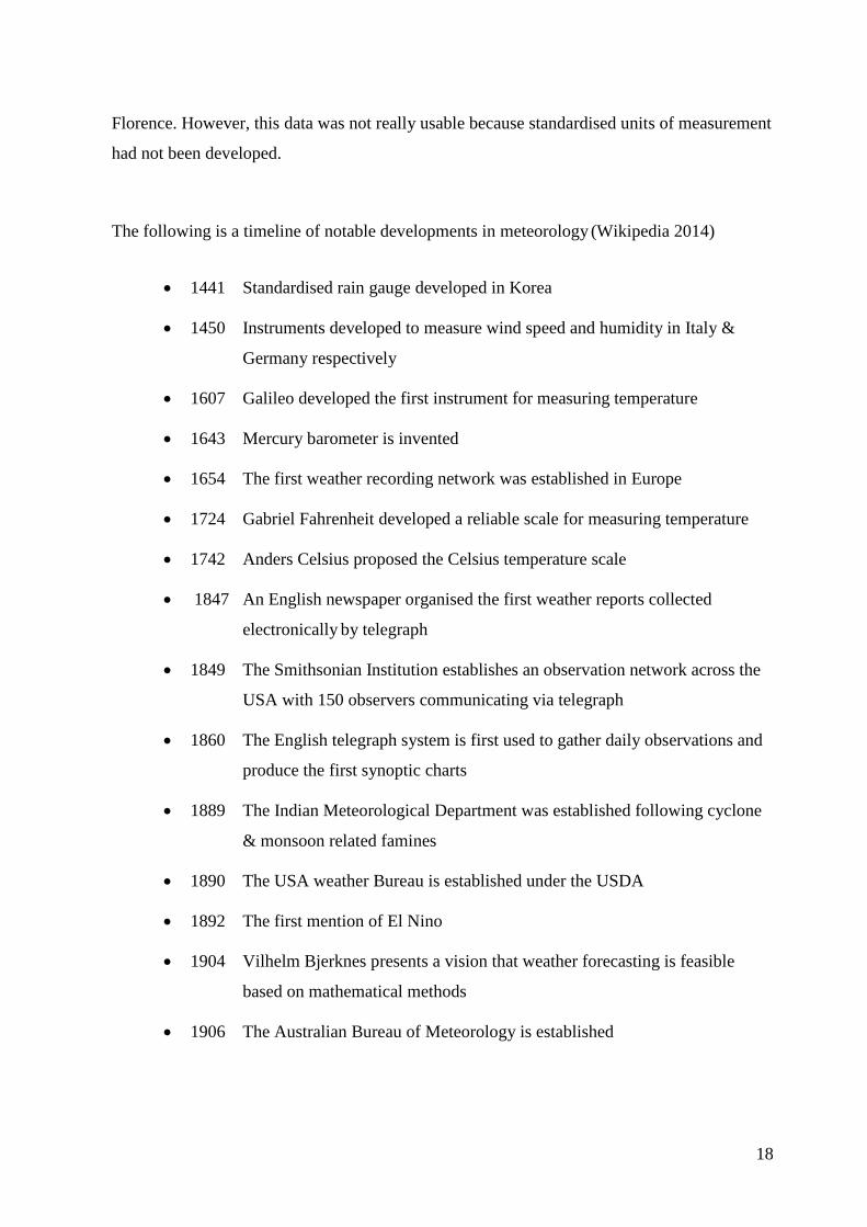
Florence. However, this data was not really usable because standardised units of measurement
had not been developed.
The following is a timeline of notable developments in meteorology (Wikipedia 2014)
1441 Standardised rain gauge developed in Korea
1450 Instruments developed to measure wind speed and humidity in Italy &
Germany respectively
1607 Galileo developed the first instrument for measuring temperature
1643 Mercury barometer is invented
1654 The first weather recording network was established in Europe
1724 Gabriel Fahrenheit developed a reliable scale for measuring temperature
1742 Anders Celsius proposed the Celsius temperature scale
1847 An English newspaper organised the first weather reports collected
electronically by telegraph
1849 The Smithsonian Institution establishes an observation network across the
USA with 150 observers communicating via telegraph
1860 The English telegraph system is first used to gather daily observations and
produce the first synoptic charts
1889 The Indian Meteorological Department was established following cyclone
& monsoon related famines
1890 The USA weather Bureau is established under the USDA
1892 The first mention of El Nino
1904 Vilhelm Bjerknes presents a vision that weather forecasting is feasible
based on mathematical methods
1906 The Australian Bureau of Meteorology is established
19
1923 The oscillation effects of ENSO were first wrongly described by Sir Gilbert
Thomas Walker from whom the Walker circulation takes its name; now an
important aspect of the Pacific ENSO phenomenon.
1941 A radar network was implemented in England during World War II.
Operators started noticing echoes from weather phenomena such as rain
and snow
1950 The first successful numerical weather prediction experiment
1969 Jacob Bjerknes described ENSO
1970’s Weather radars become more standardised and organised into networks
1975 ECMWF established
1997 The Pacific Decadal Oscillation (PDO) was discovered simultaneously by
Yuan Zhang and Steven Hare, the latter while studying salmon.
Meteorological Records
Generally, accurate meteorological records across the world are only available for the last 100
to 150 years, which is a relatively short timeframe when put into the context of the age of our
world. Efforts have been made to determine longer term climate by looking at written
observations from past civilisations, tree rings, coral growth rates and ice cores from various
parts of the world. However, in most of the information they have been used in the context of
climate change rather than in monitoring seasonal cycles and seasonal variability.
Meteorology for defence, aviation and society
Examples of how the rapid evolution of meteorology has been driven by the defence and
aviation industries include:
20
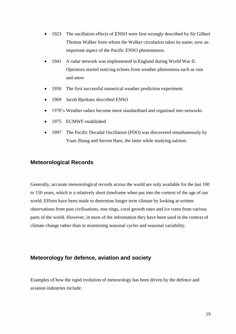
The invention of weather radar during the Second World War. The go-ahead for the
successful D-Day Normandy landings was pivotal on the weather forecast provided by
a senior meteorologist. His recommendations proved to be correct and this really
propelled forward the use of weather forecasting in the defence.
The location of weather radar has tended to be in places best suited to aviation,
defence and shipping. This can be clearly seen when viewing the map of Australia
radar locations (Figure 1).(Australian Government Bureau of Meteorology 2013)
Figure 1. Radar sites across Australia, generally located in large cities and towns for
aviation, defence and the general population. (Australian Government Bureau of Meteorology
2013 )
Teleconnections
Teleconnections can be defined as a causal connection or correlation between meteorological
or other environmental phenomena that occur a long distance apart (Australian Government
Bureau of Meteorology 2013). They were first noted by the British meteorologist Sir Gilbert
Walker in the late 19th
Century, when his studies revealed the ground breaking description of
the Southern Oscillation . (National Oceanic and Atmospheric Administration 2013)
Teleconnections are a significant part of seasonal forecasting and can help explain long term
climate variability. The following list of teleconnections is a selection of the major ones used
in mainstream weather forecasting. Canadian forecaster Ray Garnett has identified 27

21
different teleconnections for North America alone; however they are not all statistically
significant.
Teleconnections affecting Australia (and other surrounding countries)
(See Appendix 2)
Madden-Julian Oscillation (MJO)
El Nino Southern Oscillation (ENSO)
Indian Ocean Dipole (IOD)
Southern Annular Node (SAM) - Also known as the Antarctic Oscillation
Quasi Biennial Oscillation (QBO)
Other Significant Teleconnections (See Appendix 2)
North pacific Index (NP)
North Atlantic Oscillation (NAO)
Pacific Decadal Oscillation (PDO)
Arctic Oscillation (AO)
Aleutian Low
Atlantic Multi Decadal Oscillation (AMO)
It is interesting to note that one very important teleconnection discovered in recent times (the
PDO), was made at the same time by a meteorologist and a researcher studying fish. This begs
the question of what other important teleconnections are yet to be discovered and if there are
other areas in nature which could be studied by direct research.
Forcing
Recent discoveries have shown that some of the teleconnections around the world have
influence over each other, this is called forcing. Forcing can be described as the way that one
22
weather phenomenon impacts on and changes another. For example, research by Schneider et
al (Schneider & Cornuelle 2005) has pointed to a
combination of ENSO and the Aluetian Low having a forcing effect on the PDO (Appendix
2).
Astrometeorology
Astrometeorology can be defined as the theoretical effect of astronomical bodies and forces
on the Earth’s atmosphere (Ask 2014). Astrometeorologist Jenifer Lawson describes it as
“forecasting weather by studying the angular positions of the Sun, Moon and planets in
relation to each other and to the Earth; this combined influence disrupts and disturbs the
Earth's atmosphere, affecting our weather patterns.”(Lawson 2000)
As well as providing long term weather forecasts, even out to many years, astrometeorologists
also forecast earthquakes and volcanic activity. Astrometeorology has been used for
thousands of years; it has been found to be used as far back as 3,000 BC with the Sumerians
(Wikipedia 2013). Dr John Goad in 1686 was the first published astrometerologist with his
book Astro-Meteorologica. Since then astrometerologists have built on his research. Carolyn
Egan on her website “Weathersage”(Weathersage 2013) provides details of books written
about astrometeorology and offers web based courses for astrometeorology. An interesting
history of astrometeorology can be found at http://www.kimfarnell.co.uk/weather1.htm.
During research undertaken for this report, private weather forecaster Ken Ring from
Auckland, New Zealand, was interviewed. Ken uses astrometeorology as a basis for his
forecasting. In his book The Lunar Code (Ring 2006) Ken writes “During the mid seventeenth
century, scientific circles began to reject talk of planets influencing weather. With scientific
attitudes beginning to change, astrometeorology and astrology were dismissed as unscientific.
Astronomy became the only officially recognised celestial science.” Mainstream meteorology
has gradually begun to recognise some of the influences that astrometeorologists have known
for centuries.

23
Chapter 3: Weather Forecasting Methods
European Centre for Medium Range Weather Forecasting (ECMWF)
The ECMWF was established in 1975, following a severe storm surge in November 1972 that
devastated areas of Europe. It was set up to pool European scientific and technical
meteorological resources for the production of medium range weather forecasts (see
Appendix 2), resulting in both economic and social benefits to member countries.
Visiting the boardroom of the ECMWF it is immediately obvious that it is an international
organisation by the large number of flags on the table, designating the place of each of its
members. Equally obvious is the large tapestry depicting the isobars of the 1972 storm
hanging behind the chairman as a constant reminder to all members of the reason why the
centre exists (Figure 2).
Figure 2. The ECMWF boardroom showing the flags of the member countries and the
tapestry of the storm front which was the catalyst for its creation. The tapestry hangs behind
the chairman as a constant reminder to all members of why the centre exists. (Schaefer 2012)
24
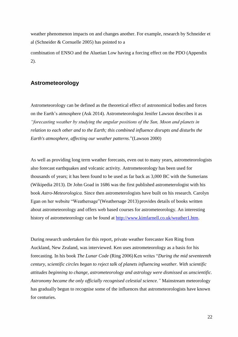
The ECMWF is known as the world leader in weather forecasting. This is clearly shown in
Figure 3, which benchmarks its performance against leading forecasting agencies around the
world. The lower the value on the y-axis denotes the lowest forecasting error.
Figure 3. A comparison of accuracy between the main international weather forecasters for
the Southern and Northern hemispheres since 1988. The closer to “1” the higher the
accuracy. (ECMWF 2012)
The ECMWF generally supplies its raw modelled data to its member partners and at a fee to
other worldwide weather forecasting agencies, including Australia.
The ECMWF uses two systems for creating their forecasts.
25
Deterministic forecasts;
The two main drivers of the improvement in weather forecasting have been the increase in
computing power and improvements in the quality and quantity of satellite data.
Deterministic forecasts are produced by computer models using a four dimensional grid
pattern to map current weather. The first two dimensions are in the horizontal plane of space –
this is made up of 16km grid points (Figure 5.). The third dimension includes 91 vertical
levels (Figure 5), and the fourth dimension is time. From these current observations the
models can model what the weather is going to do in the near future.
For example, the actual weather data is placed in the model for each grid point and the 91
vertical levels at 12.00 noon. The model determines what it estimates the actual data will be at
12.10 pm; it then uses this data to determine an estimate for 12.20 pm and so on. Each time
stamp is called a step.
The ECMWF run the deterministic forecast twice daily; each step is 600 seconds. In each of
these runs the model forecasts out to 10 days or 1440 steps. In the Northern Hemisphere the
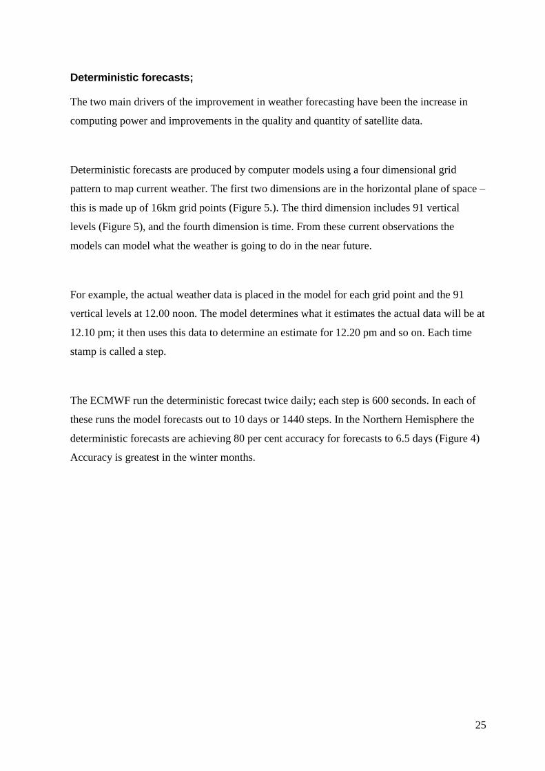
deterministic forecasts are achieving 80 per cent accuracy for forecasts to 6.5 days (Figure 4)
Accuracy is greatest in the winter months.
26
Figure 4. Chart showing the improved forecasting skill over time of ECMWF deterministic
forecasts at 80% accuracy for the Northern Hemisphere. The red line is the running average.
In 1998, this level of accuracy could be achieved only to 5 days, in 2010 it was nearly
6.5days. Notice the seasonality of the accuracy, with increased accuracy (the peaks in the
blue line) occurring during the winter period. (ECMWF 2012)
Ensemble forecasts
When meteorologists are running the deterministic model, the smaller the grid, the more
accurate the forecast, but also the more computing power is required. Furthermore real time
weather measuring stations are not located across the world on a 16km grid pattern. This
means that there are always small inaccuracies inherent in the deterministic forecast. Because
weather is extremely dynamic small changes in the accuracy of the information can
significantly affect the outcome over time. Also models cannot fully replicate the laws of
physics which govern the behaviour of the atmosphere, resulting in errors. The chaotic nature
of the atmosphere amplifies these errors over time so that initially small errors can become
extremely distorting.
The ensemble method was developed by ECMWF as a forecasting system which manages
around this inherent degree of unpredictability. Ensemble means a group of complimentary
parts or members that contribute to a single effect. An ensemble forecast in affect is a group
of deterministic forecasts that are used to provide a probability-based forecast. The ECMWF
uses a 51- member ensemble. The grid points for an ensemble forecast need to be spaced

27
further apart than the deterministic forecast due to the enormous number of calculations that
need to be made, which increases the computing power required.
Current observations are used as a base for the ensemble forecast; small errors are introduced
into each member and then the member models are run. For example, actual recorded
temperature data is available from weather recording stations located at points A & C. A is 21
degrees and C is 25 degrees, however, point B has no station. The deterministic models
predict what the conditions are at point B, for example 23 degrees. Obviously it is highly
unlikely this will be totally accurate; the error factor introduced into the ensemble members
aims to allow for these discrepancies. So one member may have B as 22.5 degrees and
another as 23.5 degrees. The ensemble forecast is run twice daily, each time with updated
real-time data. This is performed for the following 15 days.
Figure 5. The distribution of the 91 height levels used for forecasting, and the 16km
resolution as it would look over the UK for a deterministic forecast. (ECMWF 2012)
Monthly and seasonal forecasts are also performed using the ensemble method. The seasonal
forecasts are coupled with ocean data and are performed at a lower resolution due to the sheer
amount of processing required.

28
Agro Climatic Consulting
Ray Garnett is principle of Canadian based Agro Climatic Consulting. Ray grew up on a farm
and after graduating began his employment with the Canadian Wheat Board.
During 1972 a severe drought occurred in the then Soviet Union. As there was very little
information leaving the Soviet block at that time, the world was unaware of what was
transpiring. The Soviets entered the grain market and purchased a very large amount of grain
in numerous small parcels from many traders before the market realised what was happening.
This was later called the Great Grain Robbery. Following this the Canadian Wheat Board set
up a weather forecasting department to help with crop forecasting in Canada and around the
world. This is when Ray began his career in agricultural meteorology. Ray has developed a
consistent track record of forecasting and early identification of droughts and bumper harvests
in major grain growing regions around the world. In 1999 he left the Canadian Wheat Board
and established Agro Climatic Consulting. As well as publishing his own newsletter he also
writes for the Canadian grain marketing newsletter “Wild Oats”. Ray has invested a large
amount of time in researching seasonal weather forecasting and the influences behind these.
He has published seven papers as either author or co-author.
The teleconnections Ray uses include the Arctic Oscillation (AO), Bermuda High, El Nino
Southern Oscillation (ENSO), Madden-Julian Oscillation (MJO), Modified Pacific North
American Teleconnection Index (PNA), North American Snow Cover (NAS), North Atlantic
Oscillation (NAO), Pacific Decadal Oscillation (PDO), Quasi-Biennial Oscillation (QBO),
Western Pacific Teleconnection Index (WP) as well as Solar Sunspot Anomaly (SSA) Solar
index. (See Appendix 2.)
Spending time with Ray it became obvious that he is very passionate about his work and has
spent much time researching global teleconnections and their effect on grain production. Ray
has identified 27 teleconnections that affect North America. He has used a Least Angle
Regression (LARS) which is a statistical analysis to determine his top ten predictors. Ray’s
research into the solar cycle effect on our weather has produced interesting results. Ray shared

29
information (Garnett R. February 2013) from Dr. M.L. Khandekar (co-author of a paper on
Long Lead Forecasting over the Canadian Prairies) (Garnett & Khandekar 2013). Ray said
that the Magnetic North Pole moves 55 to 60km per year ((Figure 6.); this changes the earth’s
magnetic field.
Brian Vastag wrote in the National Geographic news, “in the last 150 years it has weakened
by 10%” ((Vastag B. 2005; Wikipedia 2013). Ray said Dr Khandekar also states these
changes in the pole can weaken and strengthen the affect that sunspots and the solar cycle
have on Earth’s weather by changing the amount of cosmic rays that enter our atmosphere.
Research at The European Organisation for Nuclear Research (CERN) is showing cosmic rays
may have a significant effect on cloud development (without clouds there is no rain) (Ideas
Inventions & Innovations 2013; Gosselin 2013). This is in line with a theory originally
developed by Henrik Svensmark. (Wikipedia 2013). Jasper Kirkby from CERN explains more
on that theory in his paper “Cosmic Rays and Climate” (Kirkby 2008).
Figure 6. The change in position of the earth’s North Pole over the last 174 years. (How Stuff
Works 2013)
Ray also quoted T. Landschiedt, who in his paper Trends in Pacific Decadal Oscillation
Subjected to Solar Forcing (Landscheidt 2001), showed a correlation between the PDO and
ENSO. He hypothesised that this reflected the 22 year solar cycle. Landschiedt also explained
30
that the shifts in the PDO will affect how an ENSO develops and demonstrated that there is a
close correlation between energetic solar eruptions, ENSO and the North Atlantic Oscillation
(NAO).
Ray also referenced a paper by William M Gray (Gray, Sheaffer, Knaff 1992), hypothesising
how the Quasi Biennial Oscillation (QBO) of zonal wind direction changes in the equatorial
stratosphere (middle level atmosphere), possibly affects the strength and timing of ENSO
events. Ray has proved the QBO has correlations with Australia’s weather.
Regarding his work with grain prices Ray has found that there is an inverse effect between
sunspot numbers (solar activity) and grain prices, which also tends to suggest that solar
activity is significantly affecting our weather and global grain production. He said there is a
strong correlation between the Indian Monsoon and US corn yield. There is also a strong
correlation between failed Indian Monsoon and wheat yields in Australia one to two years
later. Ray is quite frustrated that the general scientific community does not appear to be eager
to embrace the work that he and others had done on the solar influence on our weather.
Weatherquest
Located in Norwich, on the campus of the University of East Anglia, in the east of England,
Weatherquest services customers all over the UK. Weatherquest buys weather data including
ensemble forecasts from the UK Met Office then uses this data to provide a more specialised
service to its customers, which include farmers and insurance companies.
Research for this report included attending a meeting where Jim Bacon, principal of
Weatherquest spoke to farmers about the products that Weatherquest offers. His presentation
on the Ensemble Weather Forecasting System was excellent (Figure 7). The format really
helps to understand the limitations and strengths of the system and will help farmers to use it
as a tool.
31
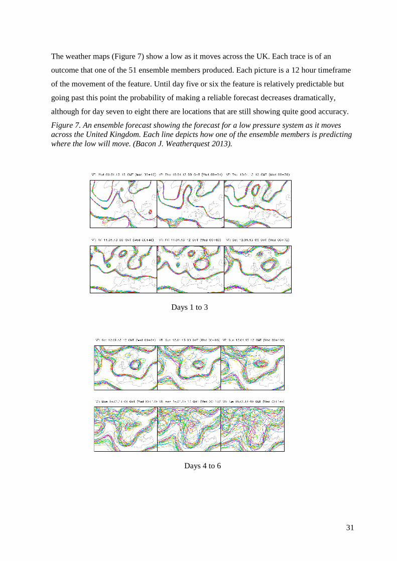
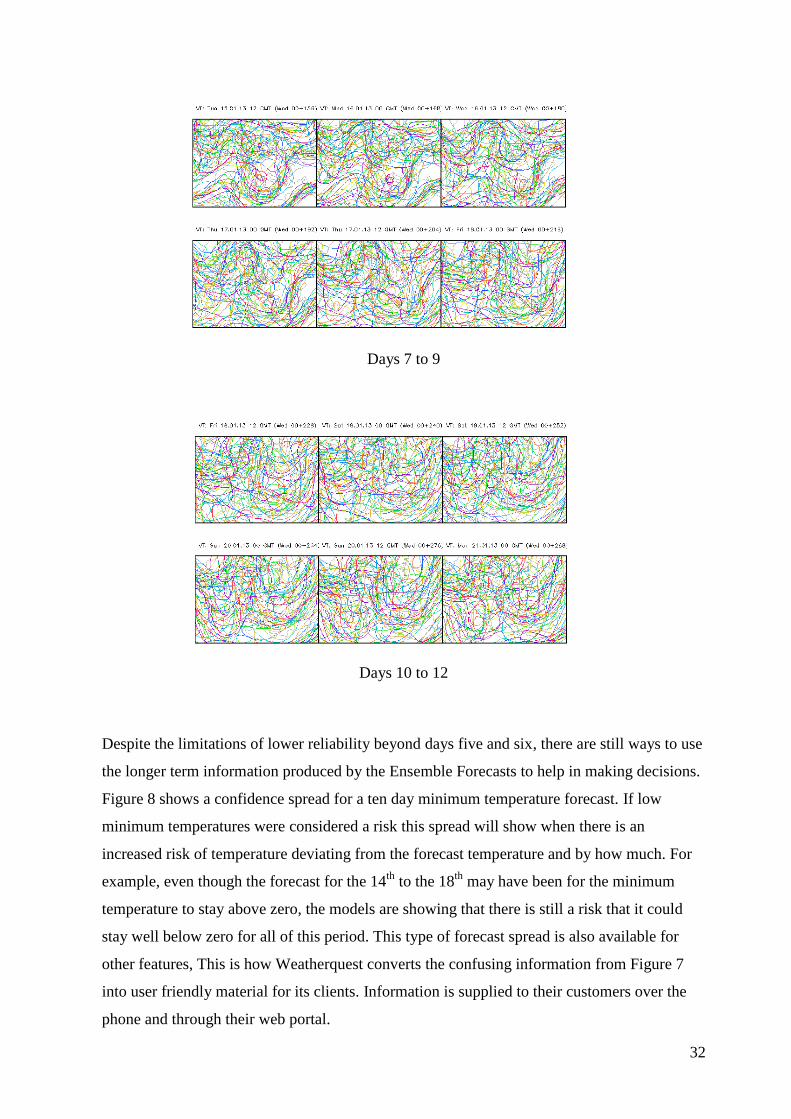
The weather maps (Figure 7) show a low as it moves across the UK. Each trace is of an
outcome that one of the 51 ensemble members produced. Each picture is a 12 hour timeframe
of the movement of the feature. Until day five or six the feature is relatively predictable but
going past this point the probability of making a reliable forecast decreases dramatically,
although for day seven to eight there are locations that are still showing quite good accuracy.
Figure 7. An ensemble forecast showing the forecast for a low pressure system as it moves
across the United Kingdom. Each line depicts how one of the ensemble members is predicting
where the low will move. (Bacon J. Weatherquest 2013).
Days 1 to 3
Days 4 to 6
32
Days 7 to 9
Days 10 to 12
Despite the limitations of lower reliability beyond days five and six, there are still ways to use
the longer term information produced by the Ensemble Forecasts to help in making decisions.
Figure 8 shows a confidence spread for a ten day minimum temperature forecast. If low
minimum temperatures were considered a risk this spread will show when there is an
increased risk of temperature deviating from the forecast temperature and by how much. For
example, even though the forecast for the 14th
to the 18th
may have been for the minimum
temperature to stay above zero, the models are showing that there is still a risk that it could
stay well below zero for all of this period. This type of forecast spread is also available for
other features, This is how Weatherquest converts the confusing information from Figure 7
into user friendly material for its clients. Information is supplied to their customers over the
phone and through their web portal.

33
For more information visit http://www.weatherquest.co.uk/aboutus.php
Figure 8. Chart showing the spread of ensemble members forecast for temperature on each
day of a 10 day forecast. The dark blue boxes show where the majority of members sit, the
lines show what the extremes are indicating. (Bacon J. Weatherquest 2013)
Oklahoma Mesonet
This is a network of interconnected, autonomous weather stations that monitor weather at a
mesoscale. Mesoscale refers to weather events varying in size between 1500m and about
240km across. They last from several minutes to several hours; because of this they might go
undetected without densely spaced weather observations.(Mesonet 2013)
Oklahoma is susceptible to all manner of extreme weather events; these include tornados,
snow storms, and heat waves of over 40oC for 60 to 80 days and ranging to winter
temperatures below -30oC.

34
The Mesonet was established in 1990 at a cost of $2.7m after the two Oklahoma Universities
joined forces and lobbied their State Government for its establishment. It is has the best
network of real time weather observation in the USA, and of anywhere visited while
researching for this report.
There are 120 observation sites evenly spaced 37 to 38km apart on a grid like pattern across
the State of Oklahoma, which has an area three quarters the size of Victoria.
The high resolution of real time data significantly improves the ability to forecast and track
severe weather events. It also improves the ability to forecast inversion conditions, which are
unsuitable for farmers undertaking pesticide application, and to provide a risk assessment of
their occurrence. Located at each site are soil moisture sensors that measure stored moisture.
This improves monitoring of soil moisture levels and rainfall deficits to help farmers assess
the risk of rainfall drought affecting their crops.
The Mesonet has developed a close relationship with emergency services managers, which
improves the planning and deployment of staff during an emergency.
Farmers are able to access Mesonet data on an interactive website
http://www.mesonet.org/index.php/agriculture/monitor and an iPhone/Android app. The
website also contains decision support tools, including a spray drift risk advisor and wheat
growth calculator, which will be discussed later in the report.
During an interview with Dr Kevin Kloesel (February 2013) at the Mesonet , the following
observation made by Mallee farmers was discussed. When a rainfall event tracks through their
district in a defined strip at the start of the cropping season it is not uncommon for that area to
receive extra rain during following rainfall events.
Dr Kloesel said that Renee McPherson had published a paper on this phenomenon
(McPherson, Stensrud. Crawford K. 2004). Apparently, rainfall, snowfall and drought all have
a “memory”. This is due to the strong theta-e (potential for convection) gradient along the
edges of the wetter land. Feedback from soil and plant characteristics can all add to the effect.
He said that current models are not able to take weather memory into account. He also said
35
that in America, much of the geophysical data that produce these phenomena is held within
the indigenous tribes of America.
Predict Weather
Predict Weather is a private weather forecasting service run by New Zealander Ken Ring. Ken
has approached weather forecasting from a very different angle.
Ken had the opportunity to observe weather from a unique perspective when living a semi-
subsistence lifestyle on the beach. He noticed a strong correlation between the tides, the moon
and weather events. He also had a close association with local Maoris and became familiar
with their fishing and farming calendars which were based on the cycles of the Moon. This
led him to researching how the moon and weather could be linked. He has also researched
links with the sun and planetary cycles. One of Ken’s frustrations is that, as soon as the moon
is mentioned, many scientists do not take him seriously, however he is able to quote many
scientific research papers to back up his methods. When asked about how the moon can
influence our weather he begins by talking about the oceans tides and the tidal mechanism. He
then points out the atmosphere actually contains more water (as water vapour) than all the
rivers and lakes on Earth put together. This still only equates to around 1% of the atmosphere,
(nitrogen is 78.09% and oxygen 20.95%). Gas by its nature is a much easier to move around
than water, so if the moon can have an effect on the oceans, Ken suggested, why should it not
affect the atmosphere?
Instead of focusing on the surface pressure as used by traditional meteorologists, Ken looks at
the total volume of the atmosphere. This expands and contracts in a tidal effect with the Moon
and to a lesser extent the Sun, and drives our weather. To add weight to this argument in his
book, The Lunar Code, (Ring K. Random House 2006) Ken mentions that astronomers have
discovered that planets without a Moon have a more stable atmosphere.
36
Regarding the Sun’s solar cycles, Ken says they are driven by the gravitational affect of the
orbits of the planets in our solar system. There is also a correlation between lunar cycles and
the solar cycle.
Looking at El Nino events in relation to these cycles Ken mentioned (March 2013) that there
are interesting correlations. In his book , he discusses how El Ninos can occur just after
sunspot minimums and around maximum, midpoint and minimum lunar declinations (where
the Moon is in relation to the north/south horizon; this has a monthly cycle as well as a longer
cycle of 18.613 years). It would be interesting to study correlations with other
teleconnections.
As well as strong supporters of his forecasting techniques in many countries, including
Australia, Ken also has some strong critics. When questioned on some of the criticisms that
have been levelled at him, Ken says many of these are brought about by misreporting, or by
his comments being taken out of context.
More information on Ken’s services can be found at www.predictweather.co.nz
Holton Weather
Ian Holton spent the first 26 years of his career with the Australian Bureau of Meteorology. In
1996 he undertook a research project to look at the influence of the Indian Ocean on
Australia’s weather. Following the publication of his paper he left the Bureau to start his own
business providing medium term and seasonal forecasts for Australian farmers.
Since those early years Ian has significantly refined his forecasting techniques. He has
continued his interest in researching weather forecasting methods and improving his
forecasting ability for his clients. A significant increase in the reliability of his forecasts
occurred in 2010 after his research uncovered strong correlations with seasonal fluctuations
and solar cycles. Ian now uses inputs from atmospheric, ocean, solar and ionospheric data.
37
Ian has also performed his own private research on human-induced climate change to see if he
needed to include an allowance for this in his forecasting models. His research has shown a
relatively small effect of the increase in atmospheric carbon dioxide on our weather.
http://www.holtonweather.com/
For the avid weather watcher Ian has also compiled a list of bush forecasting aids; this can
also be found in Appendix 1.
38
Chapter 4: The Progression of Weather
Forecasting
It is easy to dismiss the meteorologists when they supposedly “get it wrong” and to focus on
those events rather than the number of times when the forecasts are actually quite accurate.
During an interview at the ECMWF (Feb 2012), David Richardson, head of Meteorological
Operations illustrated the improvements that have occurred in weather forecasting over the
past 25 years.
Most weather forecasters are in essence mathematicians and they do their job very well. They
collect information, which is statistically analysed using various computer models. They then
try to present this information in a useable manner to a generally meteorologically uneducated
public. Sometimes the way it is presented affects the public’s perception of its accuracy.
Short term forecasting
The accuracy of the current 24 to 72 hour forecasts are quite staggering, as is the
improvement that has occurred over the past 30 years. This can be clearly seen in Figure 9.
which shows the ECMWF forecasting skill level over the past 30 years. (European Centre for
Medium Range Forecasting 2013)
39
Figure 9. Chart showing the increased forecast accuracy from 1980 to 2011 with a
comparison between Northern & Southern Hemispheres. (European Centre for Medium
Range Forecasting 2013)
The coloured area between the narrow and bold lines is the difference between the accuracy
of the southern and northern hemisphere forecasts. It can be seen that historically forecasting
accuracy for the southern hemisphere has significantly lagged behind the northern
hemisphere, until about 2001. This was due to the lack of observations; satellite data has
helped to overcome this issue.
Accuracy levels for the short term forecasts are now around 98%, which is an improvement of
25% for the southern hemisphere. It is interesting to note how the rate of improvement for
short term forecasts has slowed over the last few years, showing that it is becoming harder to
make improvements and increase the accuracy
Medium term forecasts (See Appendix 2.)
From Figure 9 the dramatic improvement in the five, seven and ten day forecasts can be seen.
In the past 13 years alone, the accuracy of the five and seven day forecasts for the southern
hemisphere has both increased by over 40%, and the ten day forecast by 20%. If the trend
lines continue as they are, the accuracies will only continue to improve.
40
Long term forecasts (See Appendix 2.)
Benchmark data for longer term and seasonal forecasting has been difficult to find. This
would tend to suggest that there is still plenty of room for improvement in this area. Darren
Ray (July 2013) from the Australian Bureau of Meteorology told me that the Bureau’s
forecasts have about a 65% accuracy.
Clients of private weather forecasters say they believe the private forecasters have a greater
skill level in this area. According to Gary McManus from the National Weather Centre in
Oklahoma, the reason for this appears to be that weather forecasters in forecasting institutions
are hesitant to use new techniques unless they are totally proven; this is especially true for
their open access products. On the other hand private forecasters tend to be much more
prepared to include a new or unusual tool if they are satisfied it will provide an increase in
forecast skill and a more accurate forecast for their clients.
Examples of this include Ray Garnett and Ian Holton who have included solar cycles and
other teleconnections in their forecasting systems, and Ken Ring who uses lunar cycles. When
Ken Ring (March 2013) was asked if he has had his forecasts benchmarked for accuracy he
made the following comment
“My accuracy has often been assessed at 80 to85%, by my clients and my own assessments,
which I am happy with, because it is enough to identify trends. Generally, the lunar method is
best suited for the timing of weather events rather than amounts of rain, which are more due
to the solar heat cycle. This is because amount of rain depends on prior evaporation rates.
An accuracy of 80 to 85% means I might be out by a couple of months over a year, or one or
two days in a week. Rain may fall within a radius of 80kms, which is both the applicability of
a report and also the error factor. This is as exact as weather forecasting can get at the best
of times because weather is typically generated about 13 to19km above the earth’s surface
and has an unavoidable overshoot factor when it reaches ground.”
41
Chapter 5: Micrometeorology
A New Science
Micrometeorology can be defined as the study of the effect on weather of the small-scale
(local) environment, generally at a resolution of about 1km or less. Micrometeorology studies
features that are too small to be depicted on a weather map. These features generally include
heat and gas movement between vegetation, soil, water and the atmosphere caused by
turbulence close to the ground.
Most current weather forecasters tend to look at the big picture (synoptic and mesonet scales)
and rarely ever consider micrometeorology in any detail. According to Australian based
private micrometeorologist Grahame Tepper (July 2012), if you were to undertake a
meteorologist course in Australia you would not encounter a micro-met subject. As far as he
is aware there are no micrometeorologist specialists in the Bureau of Meteorology either,
although there are in the CSIRO and other specialist organisations.
The difference between micrometeorology and general meteorology can be illustrated by
considering the World Meteorological Organisation (www.wmo.int/) standard for measuring
temperature. This states that temperatures should be measured at about 1.5m above the
surface in a shaded and ventilated box. This advice ensures that extremely variable
temperatures experienced at the surface are ‘evened out’ by turbulent mixing.
Micrometeorology is interested in those differences and the rates of exchange between the
surfaces and the air immediately above this height. The standard forecasting methods are only
interested in the results of the mixture of this air at about 1.5m above the surface.
Currently any micrometeorology data that is collected is not normally available to farmers. As
technology improves, with the advent of on-farm instrumentation and communications
systems and satellite-derived instantly retrievable information, it will become possible to map
microclimate variations. This will be at time scales that are useful for input into business
42
management systems, particularly in regions of complex terrain and for high yielding crops. It
will improve understanding of crop performance and management of day to day operations,
such as applying crop protectants.
Stamina, a Micrometeorology Research Project at the
Biotechnology & Biological Sciences Research Council (BBSRC)
Rothamsted
This research facility is known as the birthplace of the science of agriculture. Located south of
Cambridge in the UK, it was the site of an interesting micrometeorology research project,
overseen by Goetz Richter. As part of the Stamina project a model to research and quantify
the effect of local topography on crop yield has been developed. Sensors measuring radiation
and crop temperature were placed at canopy height and 2m above canopy height at regular
intervals down the slope. The project found that there is a strong correlation between aspect
and yield. South-facing slopes tended to be consistently lower yielding than north facing
slopes. This was found to occur because in the northern hemisphere the south-facing slopes
receive more sunlight, radiation, and the plants are hotter and become drought stressed sooner
than those on the north-facing slope. This effect would be opposite in the southern
hemisphere. The findings in regard to yield are consistent with statistical measurements of
yield maps collected from our own farm.
Dr Goetz (February 2013) said that they also found that the top of the hills tended to be lower
yielding due to the increased evaporation from more wind.
An outcome from the research was that farmers in the northern hemisphere with hill country
with a southern aspect should sow this land as well as the hilltops earlier to crops that are
faster growing, to help counteract these affects.
43
Chapter 6. Natural Climate Variability
There is a large amount of natural variability occurring within the climate. The relatively short
timescale of accurate weather records clouds the natural variability that has occurred over a
longer timescale. People’s memories and even their working lives are also relatively short, so
that they have a natural tendency to forget the bad things and remember the good. This affects
their perception.
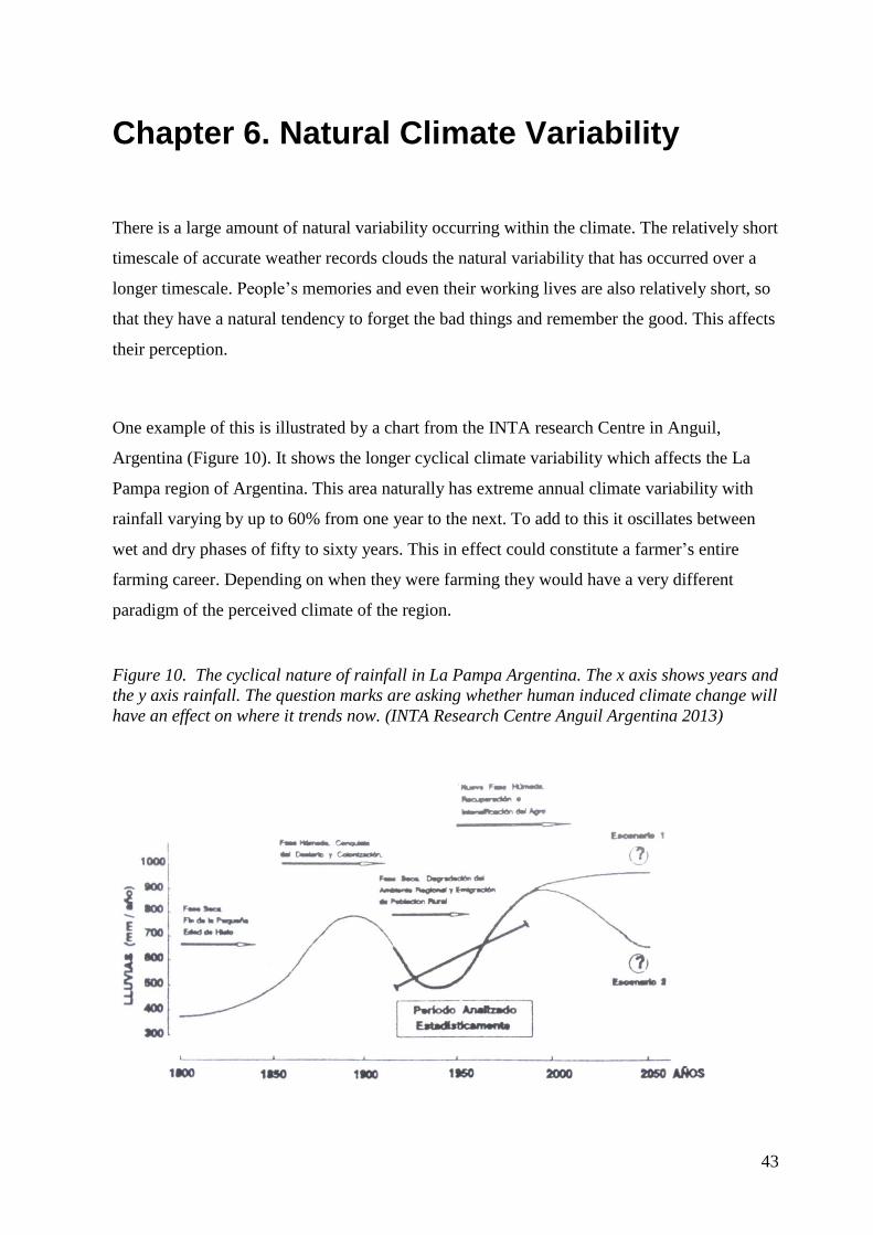
One example of this is illustrated by a chart from the INTA research Centre in Anguil,
Argentina (Figure 10). It shows the longer cyclical climate variability which affects the La
Pampa region of Argentina. This area naturally has extreme annual climate variability with
rainfall varying by up to 60% from one year to the next. To add to this it oscillates between
wet and dry phases of fifty to sixty years. This in effect could constitute a farmer’s entire
farming career. Depending on when they were farming they would have a very different
paradigm of the perceived climate of the region.
Figure 10. The cyclical nature of rainfall in La Pampa Argentina. The x axis shows years and
the y axis rainfall. The question marks are asking whether human induced climate change will
have an effect on where it trends now. (INTA Research Centre Anguil Argentina 2013)

44
Another example was presented by Chuck Cofey from the Samuel Robert Noble foundation in
Ardmore, Oklahoma. Chuck gave a presentation on the cyclical nature of Oklahoma rainfall
(February 2013). From the period 1980 to 2010 Oklahoma had a run of wetter than average
years. The question had been asked was this the “new normal”? Once the influence of the
PDO and AMO (See Appendix 2.) was understood it became apparent that the answer was no,
as this anomaly was only temporary. (Figure 11.)
Figure 11. Chart showing the influence of the PDO & AMO on Oklahoma rainfall between
1895 and 2012 (Samuel Thomas Noble Foundation 2013).
If a way can be found to look to the past to better understand climate variability in a farms
location, the land managers will be better placed to manage for the future. One example of
some work done in this area in Australia is by measuring the growth of old trees using tree
rings. In other parts of the world tree ring research has been quite extensive, however, in
Australia it is relatively new.
45
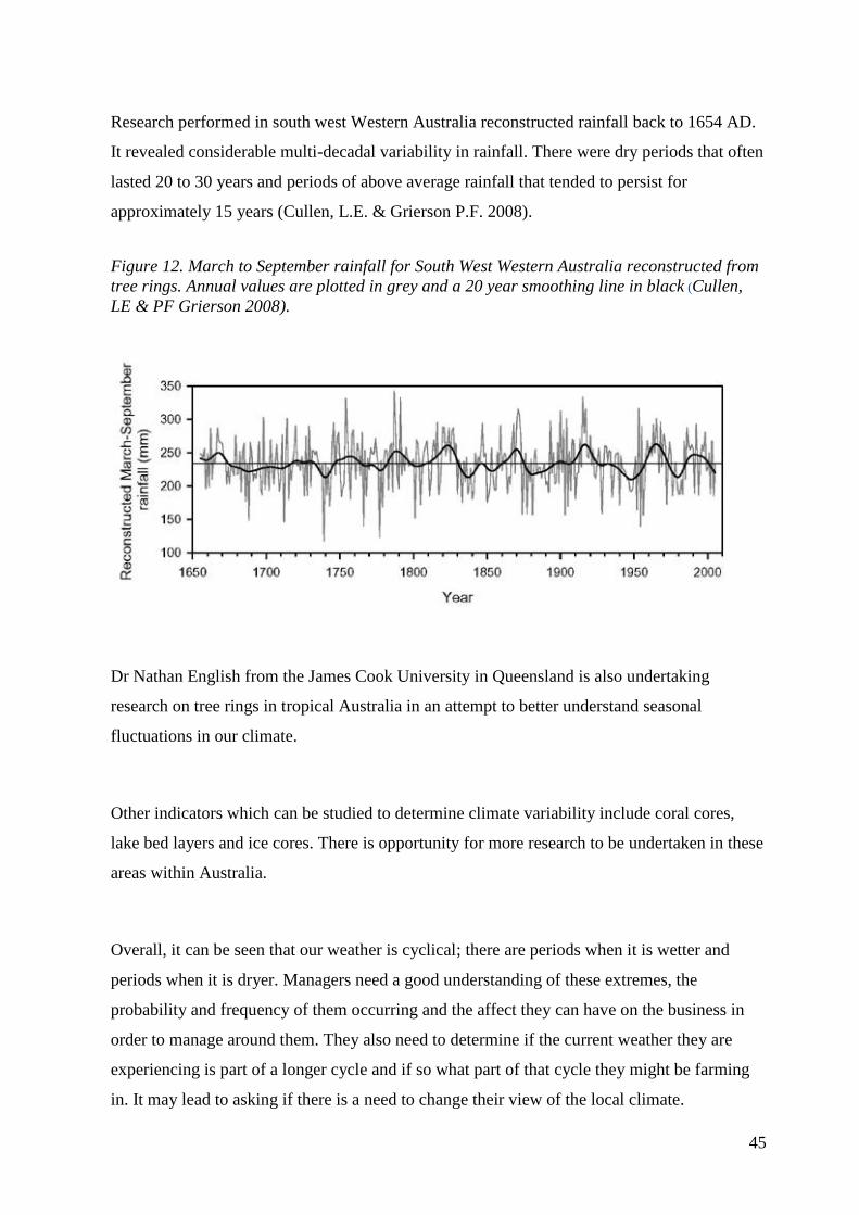
Research performed in south west Western Australia reconstructed rainfall back to 1654 AD.
It revealed considerable multi-decadal variability in rainfall. There were dry periods that often
lasted 20 to 30 years and periods of above average rainfall that tended to persist for
approximately 15 years (Cullen, L.E. & Grierson P.F. 2008).
Figure 12. March to September rainfall for South West Western Australia reconstructed from
tree rings. Annual values are plotted in grey and a 20 year smoothing line in black (Cullen,
LE & PF Grierson 2008).
Dr Nathan English from the James Cook University in Queensland is also undertaking
research on tree rings in tropical Australia in an attempt to better understand seasonal
fluctuations in our climate.
Other indicators which can be studied to determine climate variability include coral cores,
lake bed layers and ice cores. There is opportunity for more research to be undertaken in these
areas within Australia.
Overall, it can be seen that our weather is cyclical; there are periods when it is wetter and
periods when it is dryer. Managers need a good understanding of these extremes, the
probability and frequency of them occurring and the affect they can have on the business in
order to manage around them. They also need to determine if the current weather they are
experiencing is part of a longer cycle and if so what part of that cycle they might be farming
in. It may lead to asking if there is a need to change their view of the local climate.
46
Chapter 7:The Future of Weather
Forecasting
Private Sector versus Public Sector
As shown in this report there have been amazing advances in weather forecasting over the last
30 years. Short term forecasting looks like it is approaching the maximum attainable
accuracy; however, medium range and seasonal forecasting skill will continue to improve.
There is good research happening in both public and private sectors, which will continue to
improve skill levels. Research into human induced climate change is perceived to be more
important than advances in seasonal forecasting; at least advances in seasonal forecasting
seem to be a by-product of climate change research. In the places visited, there seems to be
more dedicated research into seasonal forecasting in the private sector than the public sector.
New Radar Technologies
Dual-polarization technology
One of the downfalls of current radar is that it only measures intensity of precipitation and the
direction and speed it is moving. It cannot accurately identify if it is rain, hail, snow, or ice
pellets, or measure the size of the precipitation. Dual polar radar overcomes this problem.
Conventional radar uses the return signal of a horizontal electromagnetic wave to measure the
horizontal size of an object. Dual pole radar uses a second wave sent at 45 degrees. A
computer programme separates the fields into horizontal and vertical information. This 2-D
image now provides the forecaster with the size and shape of the object. Armed with the extra
information of what the type of precipitation and how much to expect, the confidence of
forecasters to accurately assess weather events will increase. Dual pole radar is currently
being wound out in the United States and trialled at one site in Queensland.
47
Phased Array Radar
Until recently, phased array radar has only been available to the military in the United States.
Research is underway in the USA to see if civilian and military use can be combined. The
benefits of this type of radar is that it can capture 15 images in the time it takes conventional
radar to capture one. It is also able to be electronically steered, so its beam can be focused
only where storms are detected leading to faster updates. This is unlike conventional radar
that wastes time looking at clean air. Use of phased array radar would improve the lead time
associated with severe weather warning forecasts and make these forecasts more reliable.
Teleconnections
Teleconnections form a very important part of seasonal forecasting; because of their longer
term cycles they provide one of the paths to forecast future weather events. No-one
interviewed during the research for this report was specifically researching new
teleconnections; most of the teleconnections research seems to be included with other climate
research. Private forecasters such as Ray Garnett and Ian Holton are certainly doing some of
their own research. Increased research into the forcing effect of teleconnections on each other
could also provide a way to improve seasonal forecasting.
Astrometeorology
There are opportunities to further investigate the links between astrometeorology, various
teleconnections and seasonal variability, which could improve weather forecasting capabilities
Cycles
As the global weather record continues to grow we will continue to gain a better
understanding of natural cycles and variability. Further studies of tree rings, coral and

48
lakebeds will also help to give us a better understanding of these cycles. Together these will
help to understand and improve forecasting of natural cycles. As natural cycles vary in
strength there will always be a margin for error when looking at the past.
According to Chuck Coffey of the Samuel Roberts Noble Foundation (February 2013), the
current statistical models which use ENSO are based on the past, when the PDO was in a
warm phase, and El Ninos occurred every four to five years. Now that the PDO is in a cool
phase it is cycling from El Nino to La Nina and back again more frequently. So the discovery
of the PDO has really changed the way that the statistical ENSO models can be viewed, and
begs the question of what cycles are we not seeing yet and what adjustments will there need to
be made to the current models to allow for them.
Volcanic
Volcanic activity, and especially major eruptions, seem to be related in some way to the
weather. Changes in tree growth could be observed in ancient Kaori trees in New Zealand at
the times of major volcanic episodes. Some scientists suggest that this is related to
atmospheric effects from the volcanoes. Darren Ray from the Australian Bureau of
Meteorology (July 2013) said that there is documented evidence that aerosols from fires in
Indonesia are causing an increase in rainfall in Northern Australia, which would tend to
suggest that volcanic activity could also produce similar effects.
Ken Ring suggests that the volcanic activity and earthquakes can be related to the solar and
lunar cycles, which are actually driving the weather. This seems rather far-fetched, however
Ken explains that just as there is a tide at sea there is also a land tide (Earth Tide). He says the
sun and moons gravitational pull will move the land surface vertically by as much as 20 to
50cm a day. The angle and proximity of the sun, moon and indeed other planets in our solar
system, to the earth, can influence plate movement and volcanic eruptions. In a published
paper on Earth Tides (Agnew, 2007), it is suggested that earth tides can be as large as 60cm
and that as well as vertical movement there is also horizontal movement. As can be seen in
Figure 13 (A) & (B) this occurs in a global nature.
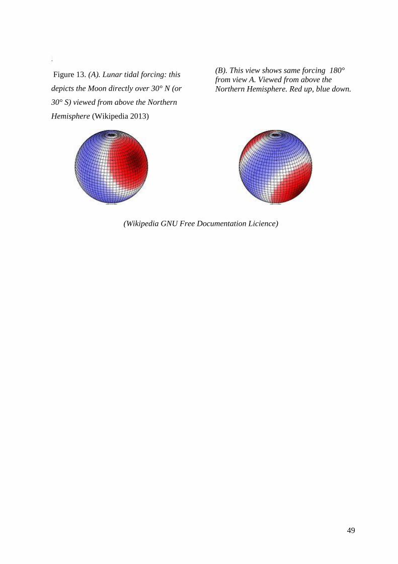
49
.
Figure 13. (A). Lunar tidal forcing: this
depicts the Moon directly over 30° N (or
30° S) viewed from above the Northern
Hemisphere (Wikipedia 2013)
(B). This view shows same forcing 180°
from view A. Viewed from above the
Northern Hemisphere. Red up, blue down.
(Wikipedia GNU Free Documentation Licience)
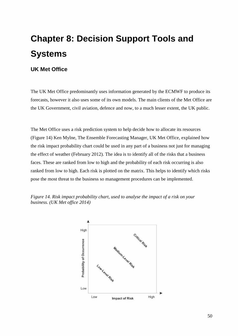
50
Chapter 8: Decision Support Tools and
Systems
UK Met Office
The UK Met Office predominantly uses information generated by the ECMWF to produce its
forecasts, however it also uses some of its own models. The main clients of the Met Office are
the UK Government, civil aviation, defence and now, to a much lesser extent, the UK public.
The Met Office uses a risk prediction system to help decide how to allocate its resources
(Figure 14) Ken Mylne, The Ensemble Forecasting Manager, UK Met Office, explained how
the risk impact probability chart could be used in any part of a business not just for managing
the effect of weather (February 2012). The idea is to identify all of the risks that a business
faces. These are ranked from low to high and the probability of each risk occurring is also
ranked from low to high. Each risk is plotted on the matrix. This helps to identify which risks
pose the most threat to the business so management procedures can be implemented.
Figure 14. Risk impact probability chart, used to analyse the impact of a risk on your
business. (UK Met office 2014)
51
Zed X
Based in Pennsylvania, USA, Zed X specialises in providing high-tech decision support
systems for a number of sectors including agriculture. The team have developed models
which combine data from global and regional forecasts that have a resolution of 30 to 60km.
In addition, the models have mesoscale observations to forecast crop development as well as
pest and disease progression in a one to ten kilometre resolution throughout the world (Figure
15). Early in the season their crop yield forecasting accuracy for the USA is within 20 to 30%,
but by mid summer (July) they are within 8 to 10% of final yield
(http://www.zedxinc.com/products/GRAIN).
Joe Russo from Zed X demonstrated how their models are able to successfully forecast when
there is an increased risk of disease or insect pressure. With this knowledge a farmer can
undertake preventative crop protection measures.
Figure 15. Diagram showing the flow of data used to generate high resolution crop and
disease forecasting by ZedX (ZedX 2012)
52
The Oklahoma Mesonet
The Mesonet has also developed some unique tools that are useful for Oklahoma farmers.
These include a Wheat Growth Calculator, Irrigation Planner, Cattle Comfort Advisor and a
Drift Risk Advisor. These products can be viewed at
http://www.mesonet.org/index.php/agriculture/monitor
With some modifications the Drift Risk Advisor is something that could be developed for
Australian farmers, which would be especially useful if it was available as an app.
Australia
The following is a brief list of Australian weather and management related systems and tools.
Climate Kelpie
This is a great point to start when looking at available tools to better understand climate and
weather. http://www.climatekelpie.com.au/
Australian Rainman
This is an excellent Australian designed tool readily available to farmers. It provides rainfall
data for 9,700 locations worldwide, for as long as records have been collected. Though it
takes a while to learn how to drive it, it is a useful tool to look at seasonal variability for the
location closest to your farm.
Australian Rainman also has a function to look at wet and dry cycles, by smoothing seasonal
rainfall over a selected number of years. It will do this for any location with long term weather
records in Australia and also has a function to import your own data. This can be helpful to
53
determine the climatic pattern that you have been farming in. It has the ability to look at
rainfall in relation to some of the teleconnections discussed. This function could certainly be
further improved in light of recent discoveries.
Australian Bureau of Meteorology (BOM)
The BOM website http://www.bom.gov.au/climate/averages/maps.shtml also has the ability to
look at historical weather data for weather stations across Australia. It is relatively easy to
navigate but lacks some of the features that Australian Rainman has which are useful for
analysing wetter and drier periods for specific locations.
Production Wise
This is production recording software which is linked to Australian Production System
Simulator (APSIM) and Yield Prophet. It has a weather and crop production forecasting
module which has some strong advocates. Recent upgrades provide users with an accuracy
assessment to give farmers more confidence in the forecasts.
Ag Seasons
The website https://www.agric.wa.gov.au/climate-land-water/climate-weather/agseasons , was
developed by The Department of Agriculture and Food Western Australia. It is targeted
specifically at Western Australian farmers. Using historical relationships between rainfall and
known teleconnections, it provides probability based forecasts for the Western Australian
(WA) grain belt. Produced at least monthly throughout the growing season, the forecasts
include an assessment of the accuracy of the forecast which is measured against historical
data. As shown in Figure 16, the forecast is map based and has a lead time of three months.
The user is able to select the start and end months of the forecast, the period in years from
which the base data will be used, and the type of forecast. The three types of forecasts which
can be selected are the most probable decile, median rainfall, and probability of exceeding
median rainfall. The website also includes features which show stored soil moisture and frost
risk for WA.
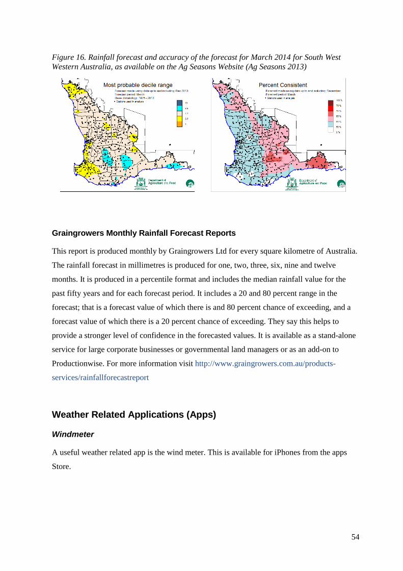
54
Figure 16. Rainfall forecast and accuracy of the forecast for March 2014 for South West
Western Australia, as available on the Ag Seasons Website (Ag Seasons 2013)
Graingrowers Monthly Rainfall Forecast Reports
This report is produced monthly by Graingrowers Ltd for every square kilometre of Australia.
The rainfall forecast in millimetres is produced for one, two, three, six, nine and twelve
months. It is produced in a percentile format and includes the median rainfall value for the
past fifty years and for each forecast period. It includes a 20 and 80 percent range in the
forecast; that is a forecast value of which there is and 80 percent chance of exceeding, and a
forecast value of which there is a 20 percent chance of exceeding. They say this helps to
provide a stronger level of confidence in the forecasted values. It is available as a stand-alone
service for large corporate businesses or governmental land managers or as an add-on to
Productionwise. For more information visit http://www.graingrowers.com.au/products-
services/rainfallforecastreport
Weather Related Applications (Apps)
Windmeter
A useful weather related app is the wind meter. This is available for iPhones from the apps
Store.
55
Australian CliMate App
This app. puts many of the functions of Australian Rainman at your fingertips. At the time of
writing it did not include a function to look at trends to understand where a location might
currently be in a weather cycle. It is certainly a helpful decision making tool.
Spraywise Decisions
Developed by Graingrowers Ltd and sponsored by Nufarm this app provides up to date
information on weather conditions for spray operators. Updated every 12 hours it forecasts
weather up to 14 days ahead, and for the first seven days, every three hours. It forecasts
temperature, wind speed and direction, relative humidity and rainfall. It is available as a
subscription service or as an add-on to Productionwise. It is also available for a free trial
http://www.spraywisedecisions.com.au/
Weatherzone+
Available for Iphones from the Apps Store this app provides the user with a twenty eight day,
seven day, and daily forecast. Also a three hourly, 48 hour forecast. It provides forecast
conditions for temperature, wind speed and direction, relative humidity and rainfall
probability. The app also has a 24 hour chart showing temperature, rainfall probability and
timing
56
Conclusion
Positioning Your Business
Given the uncertain nature of weather forecasts, the riskiest thing anyone could do is to take a
weather forecast literally. In the media we see stories of farmers who followed a forecast of a
drought literally, made a dramatic business decision, (such as deciding not to sow any crop at
all or totally de-stocking), which proved to be the correct decision and resulted in a dramatic
escape from its effects.
For every one of these stories, there are many more where a dramatic decision proved to be
incorrect resulting in huge losses. As weather forecasts continue to become more accurate
farmers will begin to increase their reliance on them. However, this could increase the risk to
the business especially when the forecast will inevitably be wrong.
A way to overcome this risk is to gather as much information as possible from a number of
sources, then to use this information to make a calculated weighted decision. For example;
given no knowledge of any weather forecasting tools, the most profit/risk balanced way to run
a business might be to always plan for an average year. However once it is known that there is
a significant chance of a below average year occurring, a percentage of resources would be
held back, so if the forecast is correct the business is better off, but if it is incorrect the
business still remains profitable. If a significant chance of an above average year was forecast,
a greater amount of resources may be allocated, increasing the profitability of the business if
the forecast proved correct, but not risking too much if an adverse season eventuated.
Managing Without Weather Forecasts
Another way to set up your business is to develop management systems that do not rely on a
weather forecast. These may be developed around obtaining better information about existing
57
conditions and working with what you know. An example of this could be planning crop
fertiliser decisions around stored moisture (or lack of) and then adjusting follow up
applications as the season unfolds. Further development of tools such as APSIM would help
this.
Further Research
This research is really only an overview of agricultural meteorology in the countries visited. It
would be really good for someone to continue this research and to look at the research
occurring in India and South Africa, especially in the area of medium range and seasonal
forecasting.
India in its own right has been researching seasonal weather forecasting for a long time.
Contacts obtained through this research project have also indicated that South Africa is
undertaking some interesting work.
Research needs to be targeted at seasonal forecasting. Investigations for this report have
confirmed there is plenty of scope to continue to improve seasonal forecasting. To achieve
this, researchers need to think outside the square, to be bold and innovative. There is evidence
to show that some of the astrometeorological forecasting techniques, like those used by Ken
Ring, may have sound scientific principles at work and warrant more investigation. An
international symposium on agricultural meteorology would be a good starting point to drive a
quicker improvement in seasonal weather forecasting.
On the opposite end of the scale to seasonal forecasting, the emerging science of micro
meteorology will become increasingly important as farmers try to manage their businesses
around constraints placed on them by the local community. Increased research to build a
better understanding of the effect of the local environment on the weather at the paddock scale
will help to reduce the risk of placing the community offside to farming practices.

58
Recommendations
Australian farmers need to improve their understanding of weather forecasting, and
understand how forecasts are generated, with their strengths and weaknesses. They also need
to know how they can make better use of the forecasts within their businesses to improve risk
management.
1. Australian meteorological research should include an open-minded focus on searching for
more teleconnections which impact Australian weather.
2. Weather forecasters need to develop better techniques to communicate forecasts to farmers
making the information even more useable.
3. Researchers and Australian Farmers need to take advantage of developments in
microprocessors for recording weather data and precision agriculture to increase knowledge in
the field of micrometeorology. Using this technology to manage the impacts of weather at a
very local level will enable farmers to improve their management of day to day operations and
reduce their impact on the local community.
4. Australia should consider hosting a worldwide symposium on Agricultural Meteorology.
59
Appendices
1. Traditional Forecasting Tools
Australian Bush Forecasting Aids
Signs that rainfall may be coming shortly to your area
Ants building high mounded ant-holes & moving eggs up on fence posts
Black clouds of flying ant swarms above treetops
Water birds nesting higher around dams & rivers
Springs starting to flow when the weather is dry
Plovers arriving earlier than normal
Emus laying eggs means rain coming in a few weeks
Lizards sitting on the top of fence posts or in trees (Facing the east in SA Mallee)
Local area kangaroos found in areas that they don't normally move through
Huntsman spiders moving inside the house, means rain in a couple of weeks
Winter type rains will start when the last leaf drops off the fig or apricot tree
Spiders silk webs floating in the air, and catching on trees, grass & fence-wire
Mice and rats moving into and/or nesting in roofs and high places
Floods in Indian sub-continent mean floods in Australia in 2 to 4 months time
Winter rains will not start until 4 to 6 weeks after the last tropical cyclone off
Western Australia
Airplane contrails remaining in sky for short periods
Frequent Whirlwinds
Dust devils turning clockwise means rain ahead...and anticlockwise means fine
weather ahead

60
Part of a list compiled by Ian Holton from information supplied by many farmers, with
thanks.
(Copyright: Ian Holton, 2007.)
United States Traditional Weather Forecasting
The Old Farmers Almanac claims an accuracy of 80% for seasonal predictions. It also
contains some interesting articles on traditional means for forecasting such as using a
persimmon seed, or a pigs spleen for more information please follow the link.
http://www.almanac.com/topics/weather/weather-forecasts/predicting-weather
How to Predict the Weather without a forecast
This is a Wiki page that is quite interesting and gives the average farmer some clues of what
to look for in nature and some scientific rationale behind why they might occur.
http://www.wikihow.com/Predict-the-Weather-Without-a-Forecast
Kenya Meteorological Department (KMD)
The KMD is working with traditional rainmakers in the Baynore community in Western
Kenya to help scientists develop more reliable systems for predicting the weather. The Nganyi
use a combination of natural phenomenon to give advice on optimal planting dates; their
reputed accuracy prompted KMD scientists to work with them. Their knowledge seems to
improve the accuracy of localised forecasts. For more information please follow the link.
http://www.new-ag.info/en/developments/devItem.php?a=2644

61
2. Terms used in this paper
Short Term Weather Forecasting
Weather forecasts for the next 48 hours
Medium Term Weather Forecasting
Weather forecasts for 3 to 14 days
Long Term Weather Forecasting
Weather forecasts longer than 14 days out to seasonal forecasts
Teleconnections affecting Australia (and other surrounding countries)
Madden-Julian Oscillation (MJO)
A global surface feature that occurs in the tropical atmosphere, it is a “pulse” of cloud and
rainfall occurring near the equator. It has an eastward movement and a typical cycle of 30 to
60 days. As it fluctuates significantly in intensity its location is not yet always measurable. It
has an influence on the development, timing and strength of the Monsoon around the world
including Australia. (Garnett R 2013)
El Nino Southern Oscillation (ENSO)
El Nino is a term used to describe warming of a large area of the central and eastern tropical
Pacific Ocean. This leads to a major change in weather patterns across the Pacific. Occurring
every three to eight years it is associated with drier conditions in Eastern Australia and wetter
conditions in parts of the USA & Canadian Prairies. ENSO is the term used to describe the
oscillation between the phases which can be in El Nino, La Nina or Neutral. There are a
number of different NINO indices that can be used to classify an ENSO event, the Australian

62
NCC uses the NINO3.4 index which you can see in Figure 17 (Garnett R 2013; Australian
Bureau of Meteorology 2013).
Figure 17. Map showing the different indices that are used around the world to classify an
ENSO event. (Australian Bureau of Meteorology 2013)
Source (45)
Recent findings in light of the discovery of the PDO have resulted in significant changes in
the way some models can be reliably interpreted. Statistical models reflect the past, when the
PDO was in a warm phase and El Ninos occurred every four to five years. Now the PDO is in
a cool phase, it is cycling from El Nino to La Nina and back again more rapidly. Statistical
models by their nature underestimate how strong El Ninos are in this new environment. They
have a bias toward the Pacific remaining in neutral for a year after a La Nina.
Dynamic models such as POAMA are more reliable since they quickly reflect every change,
however this makes them more vulnerable to the pulses of small MJO oscillations. When a
warm /dry pulse travels through El Nino, they overestimate the events strength. When a
cooler/stormy pulse flows through they underestimate. (The Browning Newsletter October
2012)
The Southern Oscillation Index (SOI) provides an indication of the development and intensity
of an El Nino or La Nina event. It is calculated using a pressure differential between Tahiti
and Darwin. A strong SOI does not necessarily indicate the severity of a drought in Australia,
however it does increase the risk of drought.
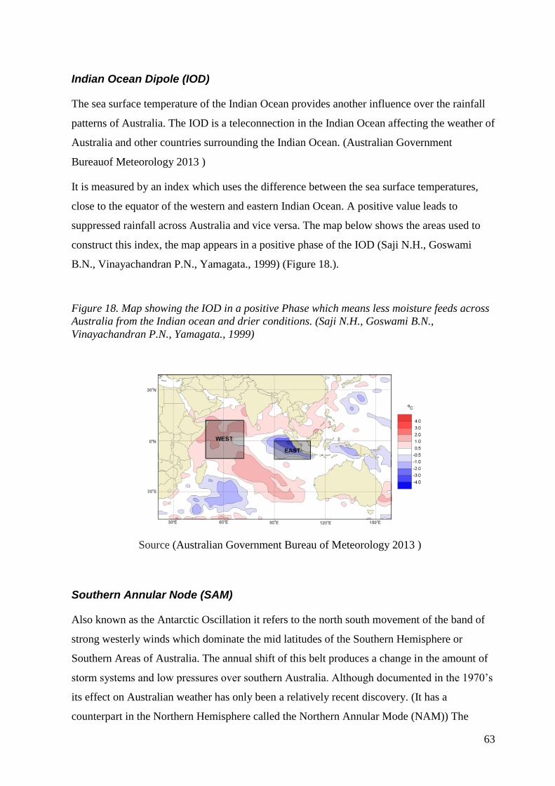
63
Indian Ocean Dipole (IOD)
The sea surface temperature of the Indian Ocean provides another influence over the rainfall
patterns of Australia. The IOD is a teleconnection in the Indian Ocean affecting the weather of
Australia and other countries surrounding the Indian Ocean. (Australian Government
Bureauof Meteorology 2013 )
It is measured by an index which uses the difference between the sea surface temperatures,
close to the equator of the western and eastern Indian Ocean. A positive value leads to
suppressed rainfall across Australia and vice versa. The map below shows the areas used to
construct this index, the map appears in a positive phase of the IOD (Saji N.H., Goswami
B.N., Vinayachandran P.N., Yamagata., 1999) (Figure 18.).
Figure 18. Map showing the IOD in a positive Phase which means less moisture feeds across
Australia from the Indian ocean and drier conditions. (Saji N.H., Goswami B.N.,
Vinayachandran P.N., Yamagata., 1999)
Source (Australian Government Bureau of Meteorology 2013 )
Southern Annular Node (SAM)
Also known as the Antarctic Oscillation it refers to the north south movement of the band of
strong westerly winds which dominate the mid latitudes of the Southern Hemisphere or
Southern Areas of Australia. The annual shift of this belt produces a change in the amount of
storm systems and low pressures over southern Australia. Although documented in the 1970’s
its effect on Australian weather has only been a relatively recent discovery. (It has a
counterpart in the Northern Hemisphere called the Northern Annular Mode (NAM)) The
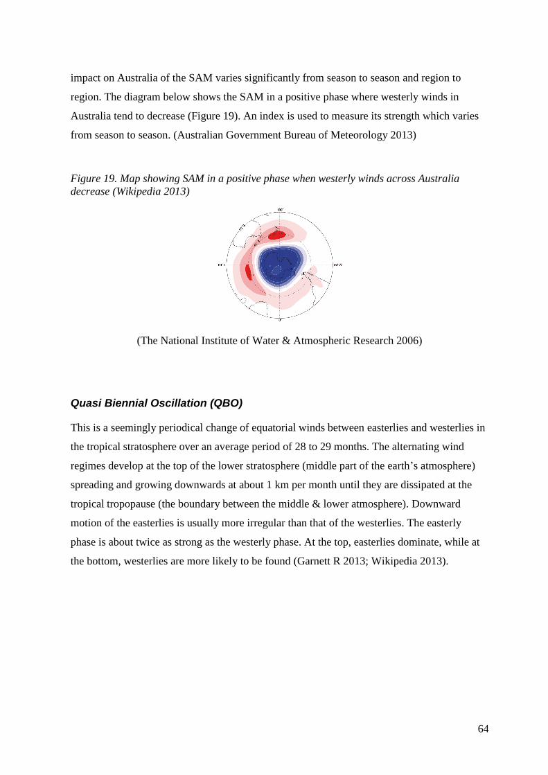
64
impact on Australia of the SAM varies significantly from season to season and region to
region. The diagram below shows the SAM in a positive phase where westerly winds in
Australia tend to decrease (Figure 19). An index is used to measure its strength which varies
from season to season. (Australian Government Bureau of Meteorology 2013)
Figure 19. Map showing SAM in a positive phase when westerly winds across Australia
decrease (Wikipedia 2013)
(The National Institute of Water & Atmospheric Research 2006)
Quasi Biennial Oscillation (QBO)
This is a seemingly periodical change of equatorial winds between easterlies and westerlies in
the tropical stratosphere over an average period of 28 to 29 months. The alternating wind
regimes develop at the top of the lower stratosphere (middle part of the earth’s atmosphere)
spreading and growing downwards at about 1 km per month until they are dissipated at the
tropical tropopause (the boundary between the middle & lower atmosphere). Downward
motion of the easterlies is usually more irregular than that of the westerlies. The easterly
phase is about twice as strong as the westerly phase. At the top, easterlies dominate, while at
the bottom, westerlies are more likely to be found (Garnett R 2013; Wikipedia 2013).
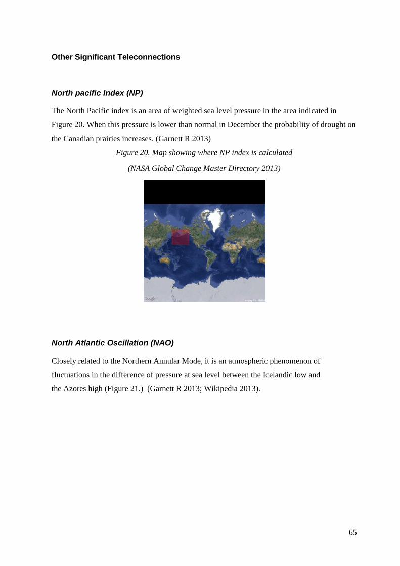
65
Other Significant Teleconnections
North pacific Index (NP)
The North Pacific index is an area of weighted sea level pressure in the area indicated in
Figure 20. When this pressure is lower than normal in December the probability of drought on
the Canadian prairies increases. (Garnett R 2013)
Figure 20. Map showing where NP index is calculated
(NASA Global Change Master Directory 2013)
North Atlantic Oscillation (NAO)
Closely related to the Northern Annular Mode, it is an atmospheric phenomenon of
fluctuations in the difference of pressure at sea level between the Icelandic low and
the Azores high (Figure 21.) (Garnett R 2013; Wikipedia 2013).
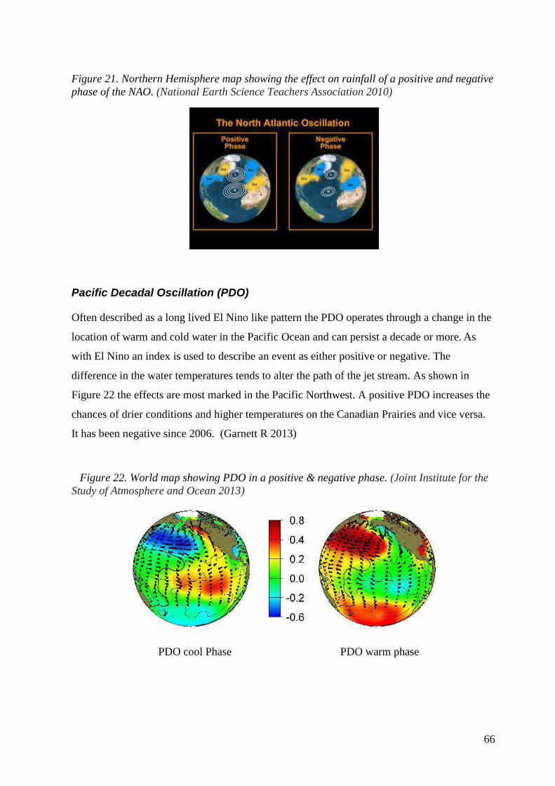
66
Figure 21. Northern Hemisphere map showing the effect on rainfall of a positive and negative
phase of the NAO. (National Earth Science Teachers Association 2010)
Pacific Decadal Oscillation (PDO)
Often described as a long lived El Nino like pattern the PDO operates through a change in the
location of warm and cold water in the Pacific Ocean and can persist a decade or more. As
with El Nino an index is used to describe an event as either positive or negative. The
difference in the water temperatures tends to alter the path of the jet stream. As shown in
Figure 22 the effects are most marked in the Pacific Northwest. A positive PDO increases the
chances of drier conditions and higher temperatures on the Canadian Prairies and vice versa.
It has been negative since 2006. (Garnett R 2013)
Figure 22. World map showing PDO in a positive & negative phase. (Joint Institute for the
Study of Atmosphere and Ocean 2013)
PDO cool Phase PDO warm phase

67
Arctic Oscillation (AO)
The Arctic Oscillation describes the degree to which arctic air penetrates into the middle
latitudes of the northern hemisphere. The Index describes the intensity of a low pressure cell
over the North Pole.
A band of upper-level winds circulates around this centre, forming a vortex (Figure 23). A
positive AO index indicates an intense vortex, the winds tighten like a noose around the North
Pole, locking cold air in place. When the opposite occurs the cold air moves southward into
North America, Europe, and Asia. The Arctic Oscillation has been mostly positive in the
wintertime since the late 1980’s and has strengthened in recent decades, contributing to the
unusual warmth over northern regions of the globe. (Garnett R 2013)
Figure 23. Showing AO in a positive and negative phase (National Snow and Ice Data Centre
2013) Credit J. Walllace University of Washington
Aleutian Low / Islandic Low
The Aleutian Low (AL) is a semi permanent low pressure centre located in the northern
hemisphere near the Aleutian Islands during the winter. The Islandic Low (IL) is also a semi
permanent low pressure centre and is located between Iceland and Southern Greenland. They
are most active during autumn and spring. They are the main centres of action in the Northern
Hemisphere atmospheric circulation. During summer they weaken, the AL retreats toward the
north pole, and the IL splits. In 2001 it was discovered that these features are connected with
an atmospheric bridge and change in strength in a seesaw pattern (Figure 24.). The variation
in the AL also affects the NAO. (Wikipedia 2013; Japanese Agency for Marine Earth and
Science Technology 2003)

68
Figure 24. Position of the Aleutian & Islandic Lows in winter and connection with the
atmospheric bridge. (Japanese Agency for Marine Earth and Science Technology 2003)
Atlantic Multi Decadal Oscillation (AMO)
The AMO is an ongoing series of long-duration changes in the sea surface temperature of the
North Atlantic Ocean, with cool and warm phases that may last for 20-40 years at a time and a
difference of about 1°F between extremes. These changes are natural and have been occurring
for at least the last 1,000 years. Since the mid-1990s we have been in a warm phase.
The AMO has affected air temperatures and rainfall over much of the Northern Hemisphere,
in particular, North America and Europe. It is associated with changes in the frequency of
North American droughts and is reflected in the frequency of severe Atlantic hurricanes.
Some scientists say it alternately obscures and exaggerates the global increase in temperatures
due to human-induced global warming (Garnett R 2013; National Oceanic and Atmospheric
Administration 2005; Wikipedia 2013).
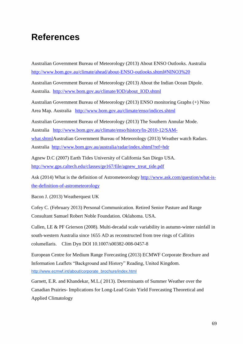
69
References
Australian Government Bureau of Meteorology (2013) About ENSO Outlooks. Australia
http://www.bom.gov.au/climate/ahead/about-ENSO-outlooks.shtml#NINO3%20
Australian Government Bureau of Meteorology (2013) About the Indian Ocean Dipole.
Australia. http://www.bom.gov.au/climate/IOD/about_IOD.shtml
Australian Government Bureau of Meteorology (2013) ENSO monitoring Graphs (+) Nino
Area Map. Australia http://www.bom.gov.au/climate/enso/indices.shtml
Australian Government Bureau of Meteorology (2013) The Southern Annular Mode.
Australia http://www.bom.gov.au/climate/enso/history/ln-2010-12/SAM-
what.shtmlAustralian Government Bureau of Meteorology (2013) Weather watch Radars.
Australia http://www.bom.gov.au/australia/radar/index.shtml?ref=hdr
Agnew D.C (2007) Earth Tides University of California San Diego USA.
http://www.gps.caltech.edu/classes/ge167/file/agnew_treat_tide.pdf
Ask (2014) What is the definition of Astrometeorology http://www.ask.com/question/what-is-
the-definition-of-astrometeorology
Bacon J. (2013) Weatherquest UK
Cofey C. (February 2013) Personal Communication. Retired Senior Pasture and Range
Consultant Samuel Robert Noble Foundation. Oklahoma. USA.
Cullen, LE & PF Grierson (2008). Multi-decadal scale variability in autumn-winter rainfall in
south-western Australia since 1655 AD as reconstructed from tree rings of Callitirs
columellaris. Clim Dyn DOI 10.1007/s00382-008-0457-8
European Centre for Medium Range Forecasting (2013) ECMWF Corporate Brochure and
Information Leaflets “Background and History” Reading, United Kingdom.
http://www.ecmwf.int/about/corporate_brochure/index.html
Garnett, E.R. and Khandekar, M.L.( 2013). Determinants of Summer Weather over the
Canadian Prairies- Implications for Long-Lead Grain Yield Forecasting Theoretical and
Applied Climatology
70
Garnett R. (2013) Glossary of Terms Used. Agro Climatic Consulting Climate and Crop
Letter June 2013. Winnipeg Canada http://www.canadagrain.com/agroclim/index.htm The
Author interviewed Garnett during his research
Garnett R (February2013) Personal Communication. Agro Climatic Consulting. Winnipeg.
Canada
Gosselin P. (2013) Jasper Kirby on the newest unpublished results of CLOUD. No Tricks
Zone. May 2013 http://notrickszone.com/2013/05/19/cerns-jasper-kirkby-on-the-newest-
unpublished-results-of-cloud-the-results-are-very-interesting/
Gray W. Sheaffer J. Knaff J.(1992) Influence of the Stratospheric QBO on ENSO Variability
Department of Atmospheric Science Colorado State University, Fort Collins USA
http://rammb.cira.colostate.edu/resources/docs/gray%20et%20al%201992.pdf
How Stuff Works (2013) Why does the north pole move.
http://science.howstuffworks.com/environmental/earth/geophysics/question782.htm
Ideas Inventions & Innovations (2013). How Cosmic Rays Make Rain
http://nanopatentsandinnovations.blogspot.com.au/2011/08/how-cosmic-rays-make-rain.html
Japanese Agency for Marine Earth and Science Technology (2003) Climate Variations
Diagnostic group. Decadal/Interdecadal climate events accompanied by the Alleutian Low.
Yokosuka Japan. http://www.jamstec.go.jp/frcgc/eng/program/cvrp/group02.html
Joint Institute for the Study of Atmosphere and Ocean (2013) The Pacific Decadal Oscillation,
Data, PDO. http://jisao.washington.edu/pdo/
Kirkby J. Cosmic Rays and Climate (2008) CERN Geneva Switzerland
http://arxiv.org/pdf/0804.1938.pdf
Kloesel K. (February 2013) Personal Communication. Director Oklahoma Climatalogical
Survey. Oklahoma University. Oklahoma. USA.
Landscheidt T. (2001) Trends in Pacific Deadal Oscillation Subjected To Solar Forcing.
Schroeter Institute for Research into Cycles of Solar Activity. Nova Scotia, Canada.
http://landscheidt.wordpress.com/papers-by-dr-theodor-landscheidt/
Lawson J. (2000) Wild Weather Forecasts 2000-2001 Nexus Magazine February-March 2000
http://cruinthe.tripod.com/nexus/articles/violentweather.html

71
McPherson R. Stensrud D. Crawford K. (2004) The Impact of Oklahoma’s winter Wheat Belt
on the Mesoscale Environment http://journals.ametsoc.org/doi/pdf/10.1175/1520-
0493(2004)132%3C0405%3ATIOOWW%3E2.0.CO%3B2Mesonet (2013) About the
Mesonet. University of Oklahoma USA http://m.mesonet.org/index.php/site/about
Mylne K. (February 2012) Personal Communication. Ensemble Forecasting Manager UK Met
office. Reading. United Kingdom.
NASA Global Change Master Directory (2013) North Pacific Index Data set Geographic
Coverage. USA. http://gcmd.nasa.gov/records/GCMD_NCAR_NP.html
National Earth Science Teachers Association. Windows to the Universe (2010) The North
Atlantic Oscillation. University at Albany USA
http://www.windows2universe.org/earth/climate/images/nao_lg_gif_image.html
National Oceanic and Atmospheric Administration (2013) USA National Weather Service
Climate prediction Centre Introduction to Teleconnections
http://www.cpc.ncep.noaa.gov/data/teledoc/teleintro.shtml
National Oceanic and Atmospheric Administration (2005). Frequently Asked Questions
About the Atlantic Multi Decadal Oscillation. Silver Spring USA.
http://www.aoml.noaa.gov/phod/amo_faq.php
National Snow & Ice Data Centre (2013) Arctic Oscillation. University of Colorado, Boulder.
USA http://nsidc.org/cryosphere/arctic-meteorology/weather_climate_patterns.html
Ray D. (July 2013) Personal Communication. Senior Meteorologist. Head of South Australian
Climate Section. Australian Bureau of Meteorology.
Richter G. (February 2013) Personal Communication. BBSRC. Rothamsted. United
Kingdom.
Ring K. (2006) The Lunar Code. Random House New Zealand
http://www.predictweather.co.nz/ShopProducts.aspx?ID=1
Ring K. (March 2013) Personal Communication. Predict Weather. Aukland. New Zealand.
Saji N.H., Goswami B.N., Vinayachandran P.N., Yamagata T., (1999): A Dipole Mode in the
Tropical Indian Ocean, Nature, 401, 360-363.
Schneider, Niklas, Cornuelle, Bruce D. 2005: The Forcing of the Pacific Decadal
Oscillation*. J. Climate, 18, 4355–4373.doi: http://dx.doi.org/10.1175/JCLI3527.1

72
Tepper G. (July 2012) Personal Communication. Private Consultant & Facilitator in Weather
Education Services for Agriculture, Aviation & Marine. Australia
The Browning Newsletter October 2012 Vol 37, No.10 http://www.browningnewsletter.com/
The National Institute of Water and Atmospheric Research. The Southern Annular Mode and
NewZealand Climate. Water and Atmosphere 2006 14 (2) Aukland NewZealand
https://www.niwa.co.nz/publications/wa/vol14-no2-june-2006/the-southern-annular-mode-
and-new-zealand-climate
Vastag B. North Magnetic Pole is Shifting Rapidly Toward Russia. National Geographic
News December 2005
http://news.nationalgeographic.com/news/2005/12/1215_051215_north_pole.html
Weathersage (2013) Reading list http://weathersage.com/about/
Wikipedia (2013) Aleutian Low http://en.wikipedia.org/wiki/Aleutian_Low
Wikipedia (2013) Atlantic Multi Decadal Oscillation
http://en.wikipedia.org/wiki/Atlantic_multidecadal_oscillation
Wikipedia (2013) Astrometeorology http://sv.wikipedia.org/wiki/Astrometeorologi
Wikipedia (2013) Earth Tide http://en.wikipedia.org/wiki/Earth_tide
Wikipedia (2013) Henrik Svensmark http://en.wikipedia.org/wiki/Henrik_Svensmark
Wikipedia (2013) North Magnetic Pole http://en.wikipedia.org/wiki/North_Magnetic_Pole
Wikipedia (2013) Quasi Biennial Oscillation http://en.wikipedia.org/wiki/Quasi-
biennial_oscillation
Wikipedia (2013) North Atlantic Oscillation
http://en.wikipedia.org/wiki/North_Atlantic_oscillation
Wikipedia (2014) Timeline of Meteorology
http://en.wikipedia.org/wiki/Timeline_of_meteorology
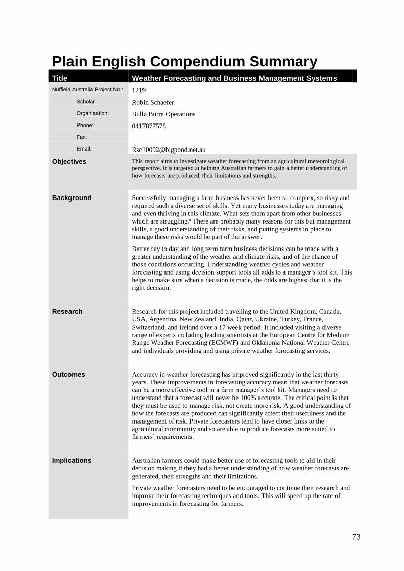
73
Plain English Compendium Summary Title Weather Forecasting and Business Management Systems
Nuffield Australia Project No.: 1219
Scholar: Robin Schaefer
Organisation: Bulla Burra Operations
Phone: 0417877578
Fax:
Email: [email protected]
Objectives This report aims to investigate weather forecasting from an agricultural meteorological
perspective. It is targeted at helping Australian farmers to gain a better understanding of
how forecasts are produced, their limitations and strengths.
Background Successfully managing a farm business has never been so complex, so risky and
required such a diverse set of skills. Yet many businesses today are managing
and even thriving in this climate. What sets them apart from other businesses
which are struggling? There are probably many reasons for this but management
skills, a good understanding of their risks, and putting systems in place to
manage these risks would be part of the answer.
Better day to day and long term farm business decisions can be made with a
greater understanding of the weather and climate risks, and of the chance of
those conditions occurring. Understanding weather cycles and weather
forecasting and using decision support tools all adds to a manager’s tool kit. This
helps to make sure when a decision is made, the odds are highest that it is the
right decision.
Research Research for this project included travelling to the United Kingdom, Canada,
USA, Argentina, New Zealand, India, Qatar, Ukraine, Turkey, France,
Switzerland, and Ireland over a 17 week period. It included visiting a diverse
range of experts including leading scientists at the European Centre for Medium
Range Weather Forecasting (ECMWF) and Oklahoma National Weather Centre
and individuals providing and using private weather forecasting services.
Outcomes Accuracy in weather forecasting has improved significantly in the last thirty
years. These improvements in forecasting accuracy mean that weather forecasts
can be a more effective tool in a farm manager’s tool kit. Managers need to
understand that a forecast will never be 100% accurate. The critical point is that
they must be used to manage risk, not create more risk. A good understanding of
how the forecasts are produced can significantly affect their usefulness and the
management of risk. Private forecasters tend to have closer links to the
agricultural community and so are able to produce forecasts more suited to
farmers’ requirements.
Implications Australian farmers could make better use of forecasting tools to aid in their
decision making if they had a better understanding of how weather forecasts are
generated, their strengths and their limitations.
Private weather forecasters need to be encouraged to continue their research and
improve their forecasting techniques and tools. This will speed up the rate of
improvements in forecasting for farmers.

74