Weakly Supervised Deep Learning for Brain Disease

This article has been accepted for inclusion in a future issue of this journal. Content is final as presented, with the exception of pagination.

IEEE TRANSACTIONS ON CYBERNETICS 1

Weakly Supervised Deep Learning for BrainDisease Prognosis Using MRI and

Incomplete Clinical ScoresMingxia Liu , Jun Zhang , Chunfeng Lian , and Dinggang Shen , Fellow, IEEE

Abstract—As a hot topic in brain disease prognosis, predictingclinical measures of subjects based on brain magnetic reso-nance imaging (MRI) data helps to assess the stage of pathol-ogy and predict future development of the disease. Due toincomplete clinical labels/scores, previous learning-based stud-ies often simply discard subjects without ground-truth scores.This would result in limited training data for learning reliableand robust models. Also, existing methods focus only on usinghand-crafted features (e.g., image intensity or tissue volume)of MRI data, and these features may not be well coordinatedwith prediction models. In this paper, we propose a weaklysupervised densely connected neural network (wiseDNN) forbrain disease prognosis using baseline MRI data and incom-plete clinical scores. Specifically, we first extract multiscale imagepatches (located by anatomical landmarks) from MRI to cap-ture local-to-global structural information of images, and thendevelop a weakly supervised densely connected network for task-oriented extraction of imaging features and joint predictionof multiple clinical measures. A weighted loss function is fur-ther employed to make full use of all available subjects (eventhose without ground-truth scores at certain time-points) fornetwork training. The experimental results on 1469 subjectsfrom both ADNI-1 and ADNI-2 datasets demonstrate that ourproposed method can efficiently predict future clinical measuresof subjects.

Index Terms—Alzheimer’s disease (AD), clinical score, diseaseprognosis, neural network, weakly supervised learning.

I. INTRODUCTION

AS THE most sensitive imaging test of the head(particularly the brain) in routine clinical practice, mag-

netic resonance imaging (MRI) allows physicians to evaluate

Manuscript received November 15, 2018; revised February 3, 2019;accepted March 7, 2019. This work was supported in part by NIH underGrant EB006733, Grant EB008374, Grant EB009634, Grant MH100217,Grant AG041721, Grant AG042599, Grant AG010129, and Grant AG030514.This paper was recommended by Associate Editor D. Goldgof. (Mingxia Liuand Jun Zhang contributed equally to this work.) (Corresponding author:Dinggang Shen.)

M. Liu, J. Zhang, and C. Lian are with the Department of Radiology andBRIC, University of North Carolina at Chapel Hill, Chapel Hill, NC 27599USA.

D. Shen is with the Department of Radiology and BRIC, University ofNorth Carolina at Chapel Hill, Chapel Hill, NC 27599 USA, and also withthe Department of Brain and Cognitive Engineering, Korea University, Seoul02841, South Korea (e-mail: [email protected]).

This paper has supplementary downloadable material available athttp://ieeexplore.ieee.org, provided by the author.

Color versions of one or more of the figures in this paper are availableonline at http://ieeexplore.ieee.org.

Digital Object Identifier 10.1109/TCYB.2019.2904186

(a) (b)

Fig. 1. Distribution of subjects with two types of clinical measures (i.e.,CDR-SB and MMSE) from ADNI-1 and ADNI-2 datasets [10] at four time-points: 1) BL; 2) 6th month (M06); 3) 12th month (M12); and 4) M24 afterthe BL time.

medical conditions of the brain and determine the presenceof certain diseases. Currently, MRI has been widely usedin computer-aided diagnosis of Alzheimer’s disease (AD)and its prodromal stage, that is, mild cognitive impairment(MCI) [1]–[6]. In particular, structural MRI provides a non-invasive solution to potentially identify abnormal structuralchanges of the brain, and helps identify AD-related imagingbiomarkers for clinical applications [1], [4], [7]–[9]. Recently,it has remained a hot topic to assess the stage of pathologyand predict future advances of AD and MCI, by estimatingclinical scores of subjects in future time using baseline (BL)MRI data.

Although several machine-learning methods have beenproposed for predicting clinical scores using BL MRI [11], acommon challenge of existing methods is the weakly labeleddata problem, that is, subjects may miss ground-truth clini-cal scores/labels at certain time-points. As shown in Fig. 1,among 805 subjects at BL time in the AD NeuroimagingInitiative-1 (ADNI-1) dataset [10], only 622 subjects and631 subjects have complete scores of clinical dementia ratingsum of boxes (CDR-SB) and mini-mental state examination(MMSE) at the 24th month (M24) after the BL time, respec-tively. Due to the nature of supervised learning, previousstudies merely discard subjects with missing clinical scores.For instance, Zhang and Shen [11] estimated 2-year changesof two clinical measures from BL MRI, using only 186 sub-jects with complete ground-truth clinical scores from ADNI-1.It is worth noting that removing subjects with missing scoreswill significantly reduce the number of training samples, thusaffecting the accuracy and robustness of prediction mod-els. Also, previous machine-learning methods usually feedpredefined representations [e.g., image intensity and tissuevolume within regions-of-interest (ROIs)] of MR images to

2168-2267 c© 2019 IEEE. Personal use is permitted, but republication/redistribution requires IEEE permission.See http://www.ieee.org/publications_standards/publications/rights/index.html for more information.

https://orcid.org/0000-0002-0598-5692

https://orcid.org/0000-0001-5579-7094

https://orcid.org/0000-0002-9319-6633

https://orcid.org/0000-0002-7934-5698


2 IEEE TRANSACTIONS ON CYBERNETICS

Fig. 2. Flowchart of the proposed weakly supervised deep learning methodfor brain disease prognosis, containing three main steps, that is, MR imagepreprocessing; multiscale patch extraction from MRI; and weakly supervisedneural network for clinical score regression.

subsequent prediction models, while these features may notbe optimal for prediction models, thus degrading the prognosisperformance.

Inspired by the recent success of deep learning tech-niques in medical image analysis [7], [12], [13], severalstudies resort to deep neural networks to extract MRI fea-tures for AD/MCI diagnosis in a data-driven manner [14]–[16].However, these methods are generally within the supervisedlearning framework and, thus, cannot directly employ subjectswith incomplete ground-truth clinical scores for network train-ing. Therefore, using all available weakly labeled data (i.e.,training subjects with incomplete ground-truth scores at cer-tain time-points) becomes an essential problem in MRI-basedbrain disease prognosis.

In this paper, we propose a weakly supervised deep neu-ral network (wiseDNN) for brain disease prognosis usingsubjects with BL MRI and incomplete ground-truth clinicalscores at multiple time-points. The schematic of our methodis shown in Fig. 2. We first preprocess all MR images, and thenextract multiscale image patches based on multiple AD-relatedanatomical landmarks. A deep convolutional neural network(CNN) is finally developed for joint prediction of multiple clin-ical scores at multiple time-points, with a unique weighted lossfunction that allows the network to learn from weakly labeledtraining data. Compared with the previous MRI-based studies,our proposed wiseDNN method can employ all available sub-jects (even though some of them may lack clinical scores atcertain time-points) for model training. Also, our anatomicallandmark-based multiscale patch extraction strategy can partlyalleviate the problem of limited data, by using image patchesother than entire 3-D MR images as the training samples.

The main contributions of this paper can be summarized asfollows. First, we develop a neural network with a weightedloss function that can employ all available weakly labeledsubjects (i.e., with incomplete ground-truth clinical scores),without discarding subjects having missing scores as in theprevious studies [11], [17]. This may help improve the robust-ness of the learned network by including more subjects inthe training process. Second, based on AD-related anatomicallandmarks, we propose to extract multiscale (rather than fixed-sized) image patches from MRI, where both small-scale andlarge-scale patches centered at each landmark are extracted.This kind of strategy helps to capture both local and globalstructural information of brain MRIs. Third, we develop a jointprediction strategy for estimating multiple clinical scores atmultiple time-points simultaneously. Such joint learning strat-egy is expected to model the inherent relationship amongdifferent scores at/across different time-points, thus helping

to improve the prediction performance. Finally, based on anMR image of a new test subject, the proposed method cansimultaneously predict four types of clinical scores at fourtime-points within 12 s, which is close to real time.

The remainder of this paper is organized as follows. Wepresent the most relevant studies in Section II. In Section III,we introduce the materials used in this paper and elaborate thedetails of our proposed method. In Section IV, we first intro-duce experimental settings and methods for comparison, andthen present experimental results of clinical score predictionon both ADNI-1 and ADNI-2 datasets. In Section V, we com-pare our method with previous studies and discuss limitationsof this paper as well as possible future research directions. Wefinally conclude this paper in Section VI.

II. RELATED WORK

In this section, we first introduce the conventional repre-sentations of structural brain MRIs, and then present recentMRI-based deep learning studies for brain disease progno-sis/diagnosis.

A. Representations of Structural Brain MR Images

Thanks to the development of neuroimaging techniques,we can directly access brain structures provided by MRIto understand the neurodegenerative underpinnings of ADand MCI [1], [4]. In the literature, many types of fea-ture representations of brain MRI have been developed forautomatic AD/MCI diagnosis and prognosis. These represen-tations can be roughly categorized into three classes, thatis, voxel-based representation; ROI-based representation; andpatch-based representation, with details given below.

1) Voxel-Based Representation: In general, voxel-basedapproaches [18]–[20] compare brain MR images by directlymeasuring local tissue [e.g., gray matter (GM), white matter(WM), and cerebrospinal fluid (CSF)] density of a brain viavoxel-wise analysis, after deformable registration of individ-ual brain images. For instance, Fan et al. [21], [22] proposedto extract volumetric features from brain regions from MRimages and applied them to AD classification and gender clas-sification. However, the voxel-based methods are often basedon the assumption of one-to-one anatomical mapping betweensubjects and Gaussian distributions of focal tissue densitiesduring statistical testing [23]. To make data fit the voxel-based model, tissue densities are blurred with large kernels atthe expense of focal accuracy, and therefore may reduce thediscriminative power of voxel-based representation for MRIs.Another disadvantage of voxel-based representation is that fea-ture dimension is often very high (e.g., millions), while thenumber of training subjects is very limited (e.g., hundreds),leading to the small-sample-size problem [24] and degradingthe performance of learned models.

2) ROI-Based Representation: Different from voxel-based features, ROI-based representations focus on mea-suring regionally anatomical volumes in predefined regionsin the brain. In particular, previous ROI-based stud-ies often employ tissue volume [11], [25]–[27], cortical


LIU et al.: WEAKLY SUPERVISED DEEP LEARNING FOR BRAIN DISEASE PROGNOSIS 3

thickness [28]–[33], hippocampal volume [34]–[36], and tis-sue density [9], [17], [31], [32], [37], [38] in specific brainregions as feature representation of MR images. However, thistype of representation requires a priori hypothesis on abnor-mal regions from a structural/functional perspective to defineregions in the brain [39], while such a hypothesis may notalways hold in practice. For example, an abnormal brain regionmight span over multiple ROIs or just a small part of anROI, so using a fixed partition for the brain could producesuboptimal learning performance.

3) Patch-Based Representation: Patch-based morphometrywas developed to detect fine anatomical changes in brainMRIs, by taking advantage of nonlocal analysis to modelthe one-to-many mapping between brain anatomies [23]. Asreported in [16], [23], [37], and [40]–[42] neurodegenerativepatterns can be presented through a patch-based analysis forassisting AD diagnosis and also evaluating the progression ofMCI. Liu et al. [37], [41] employed GM density within localpatches as the representation of MRI for AD diagnosis, usingrandomly selected patches (i.e., without localizing AD-relatedmicro-structures in the brain). Zhang et al. [6] proposed toextract morphometric features (i.e., local energy pattern [43])from image patches located by AD-related anatomical land-marks. These hand-crafted features of MRI are usually fed topredefined models (e.g., support vector machine [6], [41] andsparse representation [37]) for disease diagnosis and progno-sis. However, since feature extraction and model training areperformed independently in these methods, those pre-extractedMRI features may not be optimal for prediction models.

B. Deep Learning for Brain Disease Prognosis/Diagnosis

Recently, several deep learning methods have been proposedto automatically learn MRI features in a task-oriented manner.However, to directly feed the whole MR image into a CNNcould not generate robust models, since there are millions ofvoxels in an MR image and many brain regions may be notaffected by dementia. Hence, a common challenge in MRI-based deep learning is determining how to precisely locateinformative (e.g., discriminative between different groups)regions in brain MRIs.

To address this challenge, Zhang et al. [15] proposedto focus on three ROIs (i.e., hippocampal, ventricular, andcortical thickness surface) in brain MRI, and developeda deep CNN for predicting clinical measures of sub-jects using 2-D image patches extracted from three ROIs.Khvostikov et al. [44] employed only the hippocampal ROIand surrounding regions in brain scans (i.e., both structuralMRI and diffusion tensor imaging data) for learning a CNN.Similarly, Li et al. [14] presented a deep ordinal rankingmodel for AD classification, using the hippocampal ROI inMRIs. However, these studies use empirically defined regionsin MRI, without considering other potentially important brainregions that may be affected by brain diseases. Besides,Sarraf et al. [45] developed a 2-D CNN for identifying ADpatients from healthy controls (HCs) using both structuraland functional MRI (fMRI) data. However, they simply con-vert 3-D MR images and 4-D fMR images into 2-D slices

as the input of their networks, ignoring the important spatialinformation of slices in MRIs. More recently, Liu et al. [16],[46] proposed an anatomical landmark-based deep learningframework for AD diagnosis and MCI conversion prediction.Specifically, they first locate 3-D image patches via AD-relatedanatomical landmarks distributed throughout the brain, andthen develop a CNN for joint feature extraction from MRIand disease classification. However, a fixed size of imagepatches is used in these studies, without considering that struc-tural changes caused by dementia could vary largely amongdifferent brain regions.

Besides, most of the existing deep learning methods areperformed in a fully supervised manner, by merely discardingsubjects with missing ground-truth scores at certain time-points. To adequately employ all available subjects (eventhose without ground-truth scores at multiple time-points) formodel training, we propose a weakly supervised CNN forpredicting clinical measures based on BL MRI data. Theproposed method is different from the previous studies in [46].Specifically, in this paper, we focus on making use of weaklylabeled training subjects by developing a unique weightedloss function in the proposed neural network, while previousmethods [46] can only use fully labeled (i.e., with completeground-truth scores) training subjects. Also, this paper pro-poses to extract multiscale image patches centered at eachlandmark location to model multiscale structural informationof each brain MRI, while those in [46] only use fixed-sizedimage patches.

III. MATERIALS AND METHODS

In this section, we first introduce studied subjects and theprocedure of MR image preprocessing, and then present theproposed method in detail.

A. Subjects and Image Preprocessing

We perform experiments on 1469 subjects from two sub-sets of the public ADNI database [10], including ADNI-1and ADNI-2. Specifically, there are 805 subjects with BLstructural MRI data from ADNI-1, and 664 subjects with BLstructural MRI data from ADNI-2. Note that subjects thatappear in both ADNI-1 and ADNI-2 are directly removedfrom ADNI-2. Also, different from subjects with 1.5 T T1-weighted MRI in ADNI-1, the studied subjects in ADNI-2have 3.0 T T1-weighted MRI. That is, ADNI-1 and ADNI-2are two independent datasets in our experiments. According toseveral criteria,1 these subjects can be categorized into threeclasses, that is, AD, MCI, and HC.

For each subject, four types of clinical measures/scoresare used in the experiments: 1) CDR-SB; 2) classic ADassessment scale cognitive (ADAS-Cog) subscale with 11items (ADAS-Cog11); 3) modified ADAS-Cog with 13 items(ADAS-Cog13); and 4) MMSE. The date when subjects werescheduled to perform the screening becomes the BL time afterapproval. Also, the time-points for follow-up visits are denotedby the duration starting from the BL time. Specifically, we

1http://adni.loni.usc.edu



TABLE INUMBER OF STUDIED SUBJECTS HAVING FOUR TYPES OF CLINICAL SCORES (i.e., CDR-SB, ADAS-COG11, ADAS-COG13, AND MMSE) AT FOUR

TIME-POINTS, INCLUDING BL, M06, M12, AND M24 AFTER THE BL TIME

denote M06, M12, and M24 as the 6th month, 12th month,and 24th month after BL, respectively. All studied subjectshave MRI data at BL, while many have missing ground-truthscores at certain time-points regarding a specific clinical mea-sure. The detailed information about the studied subjects isshown in Table I.

For each structural MR image corresponding to a specificsubject, we first perform anterior commissure (AC)–posteriorcommissure (PC) correction, followed by skull stripping andcerebellum removal. We then linearly align each image to acommon Colin27 template [47], and further resample all MRimages to have the same size (i.e., 152×186×144 with a spa-tial resolution of 1×1×1 mm3). Using the N3 algorithm [48],we finally perform intensity inhomogeneity correction for eachMR image.

B. Proposed Method

In this paper, we attempt to deal with two challenging prob-lems in MRI-based brain disease prognosis, that is, how tomake full use of weakly labeled training data (i.e., subjectswith incomplete ground-truth clinical scores) and how to learninformative features of structural MR images. To this end, wedevelop a weakly supervised CNN to integrate feature extrac-tion and model learning into a unified framework, where aunique weighted loss function is used to employ all avail-able weakly labeled subjects for network training. Specifically,there are two main steps in the proposed wiseDNN method,that is, extraction of multiscale image patches and weaklysupervised neural network, with details given below.

1) Extraction of Multiscale Image Patches: While there aremillions of voxels in each brain MR image, the structuralchanges caused by dementia could be subtle, especially inthe early stage of AD (e.g., MCI). If we directly feed thewhole MR image into a deep neural network, the input datawill include too much noisy/irrelevant information, bringingdifficulty in network training based on only a limited (i.e.,hundreds) number of training subjects. Therefore, to facili-tate the network training for accurate disease prognosis, wewould like to first locate informative brain regions in eachMRI, rather than using the whole image.

Following [42], we resort to anatomical landmarks to locateAD-related regions in brain MRIs. To be specific, we apply alandmark detection algorithm [42] to generate a total of 1741anatomical landmarks defined in the Colin27 template [47].

(a) (b) (c)

Fig. 3. Illustration of K = 40 anatomical landmarks of three typical subjectsin their original image spaces: (a) AD; (b) MCI; and (c) HC, shown in threeviews (i.e., axial, sagittal, and coronal views). Each row denotes a particularview, and each column corresponds to a specific subject. RID: Roster ID.

As shown in Fig. S1 of the supplementary material, manylandmarks are spatially close to each other. To reduce theinformation redundancy and computational burden, we selectK = 40 anatomical landmarks from the original landmarkpool via the following steps. We first rank these landmarksin the ascending order according to their p-values, wheresuch p-values are generated by the landmark detection algo-rithm [42] by group comparison between AD and HC subjects.We then use a spatial Euclidean distance threshold (i.e., 20) asa criterion to control the distance between landmarks, and thetop K = 40 landmarks are finally chosen to be used in thispaper. As an illustration, we show the identified landmarkson three typical subjects in Fig. 3, while these landmarksshown in the template space can be found in Fig. S2 of thesupplementary material.

Based on these identified landmarks, we extract multiscaleimage patches located by each landmark from an inputMRI, to capture richer structural information of brain MRIs.Specifically, centered at each landmark, we extract both small-scale (i.e., with the size of 24 × 24 × 24) and large-scale (i.e.,with the size of 48×48×48) patches from each MRI. Hence,



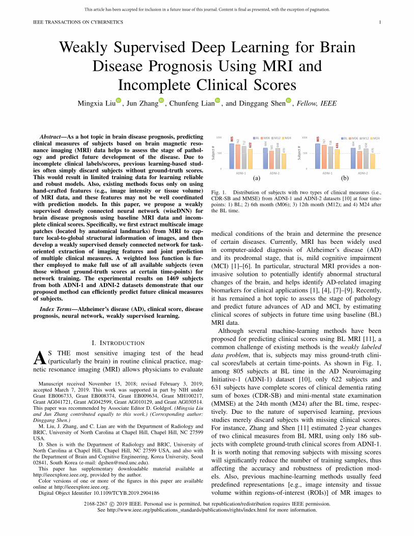
Fig. 4. Illustration of the proposed network using BL MRI data, containing K subnetworks. The input data are 2K image patches from each MR image, andthe outputs are four types of clinical scores (i.e., CDR-SB, ADAS-Cog11, ADAS-Cog13, and MMSE) at four time-points (i.e., BL, M06, M12, and M24).DCM: Densely connected module. Each DCM contains a sequence of three convolutional layers, followed by max-pooling layer for image down-sampling.

given K landmarks, we can obtain 2K image patches from eachsubject (corresponding to a particular MRI). These multiscaleimage patches will be used as the input data of our proposedneural network.

2) Weakly Supervised Neural Network: Using multiscaleimage patches from each MRI, we jointly perform featurelearning of MRIs and regression of multiple clinical scoresat four time-points via the proposed neural network (with thearchitecture given in Fig. 4). As shown in Fig. 4, the input ofthe proposed network includes 2K image patches from eachsubject, and the output contains four types of clinical measures(i.e., CDR-SB, ADAS-Cog11, ADAS-Cog13, and MMSE) atfour time-points (i.e., BL, M06, M12, and M24).

We first focus on modeling relatively local structuralinformation contained in multiscale image patches via K par-allel subnetworks, with each subnetwork corresponding to aspecific landmark location. In each subnetwork, we first down-sample the large-scale (i.e., 48 × 48 × 48) patch to have thesame size as that of the small-scale (i.e., 24 × 24 × 24) patch.Then, these two small-scale patches are treated as the two-channel input and fed into each subnetwork that contains asequence of three densely connected modules (DCMs) and twofully connected (FC) layers. There are three convolutional lay-ers in each DCM, followed by a 2×2×2 max-pooling layer forfeature map down-sampling. Particularly, for a specific convo-lutional layer in each DCM, feature maps (i.e., output imagesof each convolutional layer) of all preceding layers are used asinputs, and its own feature maps are used as inputs for all sub-sequent layers. All convolutional layers are followed by batchnormalization and rectified linear unit (ReLU) activation. It hasbeen proven that such densely connected architecture is use-ful in strengthening feature propagation, encouraging featurereuse, as well as substantially reducing the number of param-eters to be optimized in the network [49]. Even though the Kparallel subnetworks share the same architecture, their parame-ter weights are optimized independently. The motivation is thatwe would like to learn landmark-specific local features fromimage patches via K subnetworks to keep the unique localstructural information provided by each landmark location. If

those subnetworks share parameters, we would not be able tocapture the landmark-specific local structural information ofbrain MRIs via shallow subnetworks.

It is worth noting that using only each local patch individ-ually would not be able to capture the global structure of anMRI. To this end, the feature maps learned from the last KFC layers in K subnetworks are further concatenated, followedby two additional FC layers for learning local-to-global fea-ture representations of the input MR image. The final FC layer(with 32 neurons) is employed to predict four types of clinicalscores at four time-points.

Inspired by [50], we design a weighted loss function inthe proposed network, to make full use of all availableweakly labeled training subjects (with missing ground-truthclinical scores at certain time-points). We denote X =[x1, . . . , xn, . . . , xN] as the training set containing N subjects,where W is the network coefficient. For the nth (n = 1, . . . , N)subject xn, its sth (s = 1, . . . , S) ground-truth clinical scoreat the t-th (t = 1, . . . , T) time-point is denoted as ys,t

n . Theproposed objective function aims to minimize the differencebetween the predicted score f s,t(xn; W) and the ground truthys,t

n in the following:

arg minW

1

N

N∑

n=1

1∑T

t=1∑S

s=1 γs,tn

T∑

t=1

S∑

s=1

γ s,tn

× (ys,t

n − f s,t(xn; W))2 (1)

where γ s,tn is an indicator to denote whether xn is labeled

with the sth clinical score at the t-th time-point. Specifically,γ s,t

n = 1 if the ground-truth score ys,tn is available for xn; and

γ s,tn = 0, otherwise. To be specific, even when a training sub-

ject has missing scores at certain time-points and does notcontribute to the loss computation (i.e., γ s,t

n = 0), it can stillcontribute to the prediction tasks at the remaining time-pointsduring the network training. Hence, more samples can beemployed at different time-points. Using (1), we can not onlyautomatically learn feature representation of MR images in adata-driven manner but also utilize all available subjects (eventhough some of them may lack ground-truth clinical scores



at several time-points) for model training. This is differentfrom the conventional supervised methods [14], [16], [46] thatsimply discard subjects with incomplete ground-truth scores.

3) Implementation: To augment the training samples aswell as reduce the negative influence of landmark detectionerrors, we randomly sample different patches centered at eachlandmark location with displacements within a 5×5×5 cubic,and the step size is 1. Thus, a total of 125 patches centeredat each landmark can be extracted from each MRI at eachscale. Given K landmarks, we can obtain 125K combinationsof patches at each scale, with each combination being regardedas a particular sample for the proposed network. In this way,we can theoretically generate 125K samples for representingeach MR image, and these samples will be randomly used asthe input data of the proposed network. More details can befound in Fig. S4 of the supplementary material.

At the training stage, we train the network based on thetraining subjects, using their BL MRIs as input and thecorresponding ground-truth four clinical scores at four time-points (with missing values) as output. Specifically, basedon K anatomical landmarks, we first sample multiscale (i.e.,24×24×24 and 48×48×48) image patches from each trainMRI, and then feed these patches to the network. In this way,we can learn a nonlinear mapping from each input MRI to itsfour clinical scores at four time-points. At the testing stage,for an unseen test subject with only a BL MR image, we firstlocate its corresponding landmarks via the deep learning-basedlandmark detection algorithm [42], and then extract multiscalepatches based on these landmarks. Finally, we feed thesemultiscale image patches into the learned network to predictthe clinical scores at four time-points for this test subject.

We implement the proposed network using Keras [51] withTensorflow backend [52]. The objective function in (1) is opti-mized by a stochastic gradient descent (SGD) approach [53]combined with a backpropagation algorithm for computingnetwork gradients as well as parameter update. Specifically,we empirically set the momentum coefficient and the learningrate for SGD to 0.9 and 10−4, respectively. The change curvesof the training and validation loss function on the ADNI-1dataset can be found in Fig. S2 of the supplementary mate-rial. Particularly, for an unseen testing subject with BL MRI,our method requires approximately 12 s for predicting its fourtypes of clinical measures at four time-points, using a com-puter with a single GPU (i.e., NVIDIA GTX TITAN 12 GB).This implies that the proposed wiseDNN method is expected toperform real-time brain disease prognosis in real-world appli-cations. For readers’ convenience, the code and the pretrainedmodel have been made publicly available online.2

IV. EXPERIMENTS

In this section, we first present the experimental settings andintroduce the methods for comparison. We then present andanalyze the experimental results achieved by different meth-ods on both ADNI-1 and ADNI-2 datasets, and compare ourmethod with several state-of-the-art methods for MRI-basedAD prognosis.

2https://github.com/mxliu/wiseDNN

A. Experimental Settings

To investigate the robustness of the proposed method,we perform two groups of experiments in a twofold cross-validation manner. Specifically, in the first group of exper-iments, we train models on subjects from ADNI-1, and testthem on subjects from the independent ADNI-2 dataset. In thesecond group, we train models on ADNI-2 and test them onADNI-1, respectively. In the experiments, we aim to predictfour types of clinical scores (i.e., CDR-SB, ADAS-Cog11,ADAS-Cog13, and MMSE) at four time-points (i.e., BL, M06,M12, and M24), by using BL MRI data. Two criteria are usedto evaluate the performance of our method and those compet-ing approaches: 1) the correlation coefficient (CC) and 2) theroot mean square error (RMSE) between the ground-truth andthe predicted clinical scores achieved by a particular method.We also perform a paired t-test (with a significance level of0.05) on prediction results achieved by our wiseDNN methodand each specific comparison method.

B. Methods for Comparison

We first compare the proposed wiseDNN method with threeconventional feature representations of brain MRI: 1) voxel-based tissue density (denoted as Voxel) [19]; 2) ROI-basedGM volume (denoted as ROI) [11]; and 3) landmark-basedmorphological features (denoted as LMF) [42]. The details ofthese methods are introduced in the following.

1) Voxel: In this method, a nonlinear image registrationalgorithm [54] is first applied to spatially normalize allMR images to the template space. Then, the FAST algo-rithm in the FSL package [55] is employed to segmenteach MR image into three tissues (i.e., GM, WM, andCSF). Then, the local GM tissue density in each voxelis used as a feature value. The feature vector (with eachelement corresponding to a particular voxel) of eachMR image is finally fed into a support vector regres-sor (SVR) for clinical score regression. For each typeof clinical scores at a specific time-point, a linear SVR(with a default parameter C = 1) will be learned basedon training subjects and, thus, models for different scoresat different time-points are independently trained in thismethod.

2) ROI: Similar to the Voxel method, the ROI method firstsegments the GM tissue from the spatially normalizedMR image. Using a nonlinear registration algorithm, thesubject-labeled image based on the AAL template with90 manually labeled ROIs can be generated. For eachof 90 brain regions in the labeled MR image, the GMtissue volume of that region is computed as a feature.Then, a 90-D feature vector can be generated for eachMR image, and such a feature vector is then fed into alinear SVR (with a default parameter C = 1) for inde-pendent regression of different clinical scores at differenttime-points.

3) LMF: In this method, the same K landmarks as thoseused in our method are employed to locate AD-relatedimage patches in MRI. Specifically, centered at a par-ticular landmark, LMF first extracts an image patch



TABLE IIRESULTS OF CCS BETWEEN THE GROUND-TRUTH AND PREDICTED SCORES OF FOUR TYPES OF CLINICAL MEASURES, ACHIEVED BY DIFFERENT

METHODS AT FOUR TIME-POINTS (i.e., BL, M06, M12, AND M24). HERE, LEARNING MODELS ARE TRAINED AND TESTED ON ADNI-1 AND ADNI-2,RESPECTIVELY. THE BEST RESULTS ARE SHOWN IN BOLD. THE TERM DENOTED BY ∗ REPRESENTS THAT THE RESULTS OF WISEDNN

ARE STATISTICALLY SIGNIFICANTLY BETTER THAN OTHER COMPARISON METHODS (p < 0.05) USING PAIRWISE t-TEST

(24×24×24), and then compute the 100-D local energypattern [43] as features for this patch. By concatenat-ing these patch-based features, a 100K-D feature vectoris finally obtained for representing each MR image,followed by a linear SVR for clinical score regression.

Three critical strategies are used in wiseDNN, that is, jointprediction of multiple clinical scores at multiple time-points;multiscale patch extraction; and utilization of weakly super-vised subjects (with complete BL MRI data and incompleteground-truth clinical scores) for model training. To investigatethe influence of each strategy, we further compare wiseDNNwith its four variants, with details given below.

1) wiseDNN-IS, that independently trains a model for eachclinical measure using only small-scale (i.e., 24 × 24 ×24) patches. In wiseDNN-IS, we simply train an inde-pendent network for each type of clinical measure ateach time-point, with the input of small-scale imagepatches centered at K landmark locations.

2) wiseDNN-I, that learns an independent network foreach type of clinical scores using multiscale patches.Specifically, in wiseDNN-I, we separately train a spe-cific network for each type of clinical scores at eachtime-point, without exploiting the underlying relation-ship among different clinical measure and that amongdifferent time-points.

3) wiseDNN-S, that uses only small-scale patches for learn-ing a joint network for four clinical measures. In thismethod, we only extract a small-scale (24 × 24 × 24)patch from each landmark location in an MR image,without accounting for more global information of thatimage captured by large-scale (48 × 48 × 48) patches.

4) wiseDNN-C, that uses only labeled subjects (i.e.,with complete ground-truth clinical scores at fourtime-points) for network training. In other words, inwiseDNN-C, subjects with clinical scores missed atleast at one time-point will be discarded. In con-trast, wiseDNN can use all weakly labeled subjects fornetwork training via a weighted loss function in (1).For a fair comparison, similar to wiseDNN, wiseDNN-Cuses multiscale image patches for joint prediction of fourtypes of clinical scores at four time-points.

In summary, the proposed wiseDNN method is comparedwith seven methods in the experiments. Among these meth-ods, five approaches (i.e., Voxel, ROI, LMF, wiseDNN-IS,and wiseDNN-I) independently train models for different

clinical measures, while three approaches (i.e., wiseDNN-S,wiseDNN-C, and wiseDNN) jointly predict multiple clini-cal measures. In three conventional feature-based methods(i.e., Voxel, ROI, and LMF), a linear SVR (with a defaultparameter C = 1) will be learned independently for eachtype of clinical scores at each time-point. Six landmark-basedmethods (i.e., LMF, wiseDNN-IS, wiseDNN-I, wiseDNN-S,wiseDNN-C, and wiseDNN) share the same landmark pool asshown in Fig. 3. Also, four methods (i.e., Voxel, ROI, LMF,and wiseDNN-C) can only employ subjects with completeground-truth scores at four time-points, while the remain-ing ones (i.e., wiseDNN-IS, wiseDNN-I, wiseDNN-S, andwiseDNN) can take advantage of all available training sub-jects (even though some of them may lack clinical scores atcertain time-points).

C. Prognosis Results on ADNI-2

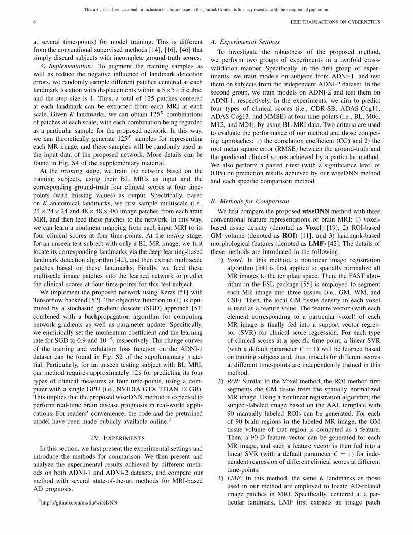
In this group of experiments, we train models on ADNI-1,and test them on ADNI-2. In Table II, we report the CCvalues achieved by eight different methods, with ∗ denotingthat the results of wiseDNN are statistically significantly bet-ter than other compared methods (p < 0.05) using pairwiset-test. Besides, the RMSE values obtained by different meth-ods are reported in Fig. 5. We further show scatter plots of theground-truth versus predicted scores achieved by our proposedwiseDNN method in Fig. 6. From Table II and Figs. 5 and 6,one could have the following observations.

1) Methods (i.e., wiseDNN-IS, wiseDNN-I, wiseDNN-S,wiseDNN-C, and wiseDNN) using task-oriented fea-tures via neural networks usually yield better results(regarding both CC and RMSE), compared with meth-ods (i.e., Voxel, ROI, and LMF) using hand-craftedfeatures of MRI. Also, even though LMF employs thesame landmarks as wiseDNN to locate patches in MRI,its performance is worse than that of wiseDNN. Forinstance, LMF achieves a CC value of 0.431, which isworse than that (i.e., 0.539) of wiseDNN in predictingCDR-SB at BL. This may occur due to that LMF usesexpert defined features of MRI for disease prognosis,where these features may not be well coordinated withsubsequent prediction models. These findings imply thatthe integration of feature extraction into model learning(as we do in this paper) helps improve the prognosisperformance.



(a) (b)

(c) (d)

Fig. 5. Results of RMSE between the ground-truth and predicted clinical scores achieved by eight different methods at four time-points: (a) BL; (b) M06;(c) M12; and (d) M24. Here, learning models are trained and tested on ADNI-1 and ADNI-2, respectively.

(a)

(b)

(c)

(d)

Fig. 6. Scatter plots of ground-truth versus predicted scores of: (a) CDR-SB; (b) ADAS-Cog11; (c) ADAS-Cog13; and (d) MMSE at four time-points,achieved by the proposed wiseDNN method. Each row denotes a particular clinical measure, and each column denotes a time-point. Here, the proposed neuralnetwork is trained and tested on ADNI-1 and ADNI-2, respectively.

2) Compared with those methods (i.e., Voxel, ROI,wiseDNN-IS, and wiseDNN-I) that independently learnmodels for different clinical scores, the proposed meth-ods (i.e., wiseDNN-S, wiseDNN-C, and wiseDNN) thatjointly predicting multiple scores generally yield higherCC and lower RMSE values. It suggests that our jointlearning strategy could boost the learning performance,

by implicitly exploiting the inherent relationship amongdifferent clinical measures.

3) Methods (i.e., wiseDNN-C and wiseDNN) usingmultiscale image patches consistently outperform theircounterparts (i.e., wiseDNN-IS and wiseDNN-S) usingonly single-scale patches, in terms of both CCand RMSE values. Thanks to both small-scale and



TABLE IIIRESULTS OF CCS BETWEEN THE GROUND-TRUTH AND PREDICTED SCORES OF FOUR TYPES OF CLINICAL MEASURES, ACHIEVED BY EIGHT

DIFFERENT METHODS AT FOUR TIME-POINTS (i.e., BL, M06, M12, AND M24). HERE, LEARNING MODELS ARE TRAINED AND TESTED ON ADNI-2AND ADNI-1, RESPECTIVELY. THE BEST RESULTS ARE SHOWN IN BOLD. THE TERM DENOTED BY ∗ REPRESENTS THAT THE RESULTS OF WISEDNN

ARE STATISTICALLY SIGNIFICANTLY BETTER THAN OTHER COMPARISON METHODS (p < 0.05) USING PAIRWISE t-TEST

(a) (b)

(c) (d)

Fig. 7. Results of RMSE between the ground-truth and predicted clinical scores achieved by eight different methods at four time-points: (a) BL; (b) M06;(c) M12; and (d) M24. Here, learning models are trained and tested on ADNI-2 and ADNI-1, respectively.

large-scale image patches, wiseDNN-C and wiseDNNcan model more global structure information of MRI,while wiseDNN-IS and wiseDNN-S merely focus onlocal information of MRI via single-scale patches. Thiscould partly explain why using multiscale image patchescan generate better prediction results.

4) The performance of each method slightly decreases overtime in predicting four types of clinical scores. As anexample, wiseDNN obtains an RMSE value of 3.408at M24, which is worse than that (i.e., 2.554) at BLin predicting MMSE. This result may be caused by thefact that we only use BL MRI data to predict clinicalscores at four time-points, while the brain structure mayslightly change along time after BL time. A more reason-able solution is to use MRI at multiple time-points forpredicting clinical scores at different time-points, whichis expected to generate better performance.

D. Prognosis Results on ADNI-1

In the second group of experiments, we train and test learn-ing models on ADNI-2 and ADNI-1, respectively. The CCand RMSE values achieved by different methods are shownin Table III and Fig. 7, respectively. From Table III and Fig. 7,we can see that, in most cases, our proposed wiseDNN methodachieves better performance than the competing methods,regarding both CC and RMSE values.

Besides, it can be observed from Tables II and III andFigs. 5 and 7 that wiseDNN is superior to wiseDNN-C in

predicting four types of clinical scores at four time-points.Note that wiseDNN uses all subjects with incomplete ground-truth scores for model training, while wiseDNN-C employsonly subjects with complete scores. These results imply thatusing all available weakly labeled subjects for model learning,as we do in wiseDNN, provides a good solution to improve theprognosis performance. Also, Tables II and III suggest that theproposed wiseDNN method achieves comparable results usingindependent models trained on ADNI-1 and ADNI-2, respec-tively. This implies that our method has a good generalizationability because MRIs in ADNI-1 and ADNI-2 were acquiredby 1.5 T and 3.0 T scanners, respectively.

In addition, we can see from Tables II and III that the over-all correlation between the estimated scores achieved by alleight methods and the ground-truth scores are not high, andhence these methods are not yet ready to be used in a clinicalsetting. The underlying reason could be that the brain MRIsof subjects within four categories (AD, pMCI, sMCI, and HC)are combined for network training. Note that it is challengingto accurately distinguish between four categories, because theAD-related structural changes of the brain could be very sub-tle. Besides, MCI is the early stage of AD, and many MCIsubjects (such as sMCI) will not necessarily convert to AD,leading to the complex data distribution of four categories.

E. Comparison With the State-of-the-Art Methods

In the literature, several methods have been proposed topredict clinical scores at multiple time-points [11], [46].



(a)

(b)

Fig. 8. Comparison between the proposed wiseDNN method and two state-of-the-art methods (i.e., M3TL in [11] and DM2L in [46]) in estimating twotypes of clinical scores (i.e., ADAS-Cog11 and MMSE) at two time-points(i.e., BL and M24), in terms of (a) CC and (b) RMSE. The models are trainedon ADNI-1 and tested on ADNI-2, respectively.

However, there are at least two major differences betweenour wiseDNN method and the conventional studies [11], [46].Specifically, our wiseDNN method can automatically learn dis-criminative feature representations for MR images via a deepCNN, rather than using hand-crafted features (ROI-based GMtissue volume) [11]. Also, different from [11] and [46] that useonly training subjects with complete ground-truth labels/scores,wiseDNN can utilize all weakly labeled (i.e., with incompleteground-truth clinical scores) subjects for model learning, thussignificantly increasing the number of training subjects andpotentially boosting the diagnosis performance.

For comparison, we further report the prognosis resultsachieved by wiseDNN and these two previous methods, that is,multimodal multitask learning (M3TL) [11] and deep multitaskmultichannel learning (DM2L) [46]. Note that, M3TL relies onan independent linear SVR for clinical score regression at eachtime-point, while both DM2L and our wiseDNN methods per-form the joint regression of multiple clinical scores via CNNs.For predicting two types of clinical scores (i.e., ADAS-Cog11and MMSE) at two time-points (i.e., BL and M24), models inthis group of experiments are trained on ADNI-1 and tested onADNI-2, respectively. Both M3TL and DM2L can only employsubjects with complete ground-truth clinical scores for modeltraining, while our wiseDNN method is capable of using allavailable subjects.

In Fig. 8, we report the CC and RMSE values in termsof the ground-truth and estimated clinical scores achieved bythree different methods. It can be observed from Fig. 8 thatour wiseDNN method outperforms M3TL and DM2L in mostcases, further suggesting the effectiveness of our proposedmethod. Besides, compared with M3TL that uses conventionalhand-crafted features of MRI, two deep learning methods(i.e., DM2L and wiseDNN) consistently yield higher CC andlower RMSE values, further suggesting that incorporating task-oriented feature learning into the process of training prognosismodels can further improve the learning performance.

V. DISCUSSION

In this paper, we propose a wiseDNN for simultaneousprediction of multiple clinical scores at multiple time-points,

Fig. 9. Results achieved by the proposed wiseDNN method using differentnumbers of landmarks in MMSE score regression at four time-points, in termsof (left) CC and (right) RMSE. In this group of experiments, we train thenetwork on ADNI-1 and test it on ADNI-2.

using subjects with BL MRI data and incomplete ground-truthscores. This method is potentially useful in clinical practicefor disease prognosis in a fast and objective way. For instance,given a subject who is suspected to have AD or MCI evaluatedby a physician, we can acquire the BL brain MR image. Usingthe proposed framework, we can feed this BL MRI to thetrained network to predict how the clinical status changes overtime for this patient, requiring only about 12 s. In the follow-ing, we analyze the influence of parameters and the effect ofdifferent network architectures, and then present the limitationof this paper and possible future research direction.

A. Parameter Analysis

We now evaluate the effect of the number of landmarkson the performance of the proposed wiseDNN method. In thisgroup of experiments, we vary the number of landmarks in therange of [10, 20, . . . , 60], and record the CC and RMSE resultsachieved by wiseDNN in MMSE regression. The experimentalresults are shown in Fig. 9, with models trained and tested onADNI-1 and ADNI-2, respectively.

From Fig. 9, we can observe that wiseDNN with lessthan 20 landmarks does not produce satisfactory results. Theunderlying reason could be that using a limited number oflandmarks are not able to effectively capture global struc-tural information of the brain MRI, thus leading to suboptimallearning performance. Besides, using more landmarks (e.g.,30), the results of our method are stable. Considering the com-putational burden, the optimal number of landmarks for ourmethod can be selected in the range of [30, 50].

B. Effect of Densely Connected Module

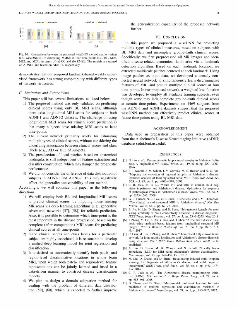
In the proposed network shown in Fig. 4, we employ threeDCMs in each subnetwork to learn patch-level local features.To study the influence of these DCMs, we further performa group of experiments by replacing three DCMs with threeresidual learning modules (RLMs) [56] and denote this newnetwork as wiseDNN-R. Note that wiseDNN-R and wiseDNNshare the same input and objective functions. In Fig. S5 ofthe supplementary material, we show the network architectureof wiseDNN-R. The experimental results produced by bothwiseDNN and wiseDNN-R in estimating MMSE scores at fourtime-points are reported in Fig. 10. It can be seen from Fig. 10that wiseDNN-R achieves similar results with wiseDNN. This



(a) (b)

Fig. 10. Comparison between the proposed wiseDNN method and its variant(i.e., wiseDNN-R) in estimating MMSE at four time-points (i.e., BL, M06,M12, and M24), in terms of (a) CC and (b) RMSE. The models are trainedon ADNI-1 and tested on ADNI-2, respectively.

demonstrates that our proposed landmark-based weakly super-vised framework has strong compatibility with different typesof network structures.

C. Limitation and Future Work

This paper still has several limitations, as listed below.1) The proposed method was only validated on predicting

clinical scores using only BL MRI scans, althoughthere exist longitudinal MRI scans for subjects in bothADNI-1 and ADNI-2 datasets. The challenge of usinglongitudinal MRI scans for clinical score prediction isthat many subjects have missing MRI scans at latertime-points.

2) The current network primarily works for estimatingmultiple types of clinical scores, without considering theunderlying association between clinical scores and classlabels (e.g., AD or HC) of subjects.

3) The preselection of local patches based on anatomicallandmarks is still independent of feature extraction andclassifier construction, which may hamper the prognosticperformance.

4) We did not consider the difference of data distribution ofsubjects in ADNI-1 and ADNI-2. This may negativelyaffect the generalization capability of our method.

Accordingly, we will continue this paper in the followingdirections.

1) We will employ both BL and longitudinal MRI scansto predict clinical scores, by imputing those missingMR scans via deep learning algorithms (e.g., generativeadversarial networks [57], [58]) for reliable prediction.Also, it is possible to determine which time-point is themost important in the disease progression, based on thecomplete (after computation) MRI scans for predictingclinical scores at all time-points.

2) Since clinical scores and class labels for a particularsubject are highly associated, it is reasonable to developa unified deep learning model for joint regression andclassification.

3) It is desired to automatically identify both patch- andregion-level discriminative locations in whole brainMRI, upon which both patch- and region-level featurerepresentations can be jointly learned and fused in adata-driven manner to construct disease classificationmodels.

4) We plan to design a domain adaptation method fordealing with the problem of different data distribu-tion [59], [60], which is expected to further improve

the generalization capability of the proposed networkfurther.

VI. CONCLUSION

In this paper, we proposed a wiseDNN for predictingmultiple types of clinical measures, based on subjects withBL MRI data and incomplete ground-truth clinical scores.Specifically, we first preprocessed all MR images and iden-tified disease-related anatomical landmarks via a landmarkdetection algorithm. Based on each landmark location, weextracted multiscale patches centered at each landmark. Usingimage patches as input data, we developed a densely con-nected neural network to simultaneously learn discriminativefeatures of MRI and predict multiple clinical scores at fourtime-points. In our proposed network, a weighted loss functionwas developed to employ all available training subjects, eventhough some may lack complete ground-truth clinical scoresat certain time-points. Experiments on 1469 subjects fromthe ADNI-1 and ADNI-2 datasets suggest that the proposedwiseDNN method can effectively predict clinical scores atfuture time-points using BL MRI data.

ACKNOWLEDGMENT

Data used in preparation of this paper were obtainedfrom the Alzheimer’s Disease Neuroimaging Initiative (ADNI)database (adni.loni.usc.edu).

REFERENCES

[1] N. Fox et al., “Presymptomatic hippocampal atrophy in Alzheimer’s dis-ease. A longitudinal MRI study,” Brain, vol. 119, no. 6, pp. 2001–2007,1996.

[2] R. I. Scahill, J. M. Schott, J. M. Stevens, M. N. Rossor, and N. C. Fox,“Mapping the evolution of regional atrophy in Alzheimer’s disease:Unbiased analysis of fluid-registered serial MRI,” Proc. Nat. Acad. Sci.USA, vol. 99, no. 7, pp. 4703–4707, 2002.

[3] C. R. Jack, Jr., et al., “Serial PIB and MRI in normal, mild cog-nitive impairment and Alzheimer’s disease: Mplications for sequenceof pathological events in Alzheimer’s disease,” Brain, vol. 132, no. 5,pp. 1355–1365, 2009.

[4] G. B. Frisoni, N. C. Fox, C. R. Jack, P. Scheltens, and P. M. Thompson,“The clinical use of structural MRI in Alzheimer disease,” Nat. Rev.Neurol., vol. 6, no. 2, pp. 67–77, 2010.

[5] B. Jie, M. Liu, D. Zhang, and D. Shen, “Sub-network kernels for mea-suring similarity of brain connectivity networks in disease diagnosis,”IEEE Trans. Image Process., vol. 27, no. 5, pp. 2340–2353, May 2018.

[6] J. Zhang, M. Liu, L. An, Y. Gao, and D. Shen, “Alzheimer’s disease diag-nosis using landmark-based features from longitudinal structural MRimages,” IEEE J. Biomed. Health Inf., vol. 21, no. 6, pp. 1607–1616,Nov. 2017.

[7] C. Lian, M. Liu, J. Zhang, and D. Shen, “Hierarchical fully convolutionalnetwork for joint atrophy localization and Alzheimer’s disease diagnosisusing structural MRI,” IEEE Trans. Pattern Anal. Mach. Intell., to bepublished.

[8] X. Liu, D. Tosun, M. W. Weiner, and N. Schuff, “Locally linearembedding (LLE) for MRI based Alzheimer’s disease classification,”NeuroImage, vol. 83, pp. 148–157, Dec. 2013.

[9] M. Liu, D. Zhang, and D. Shen, “Relationship induced multi-templatelearning for diagnosis of Alzheimer’s disease and mild cognitiveimpairment,” IEEE Trans. Med. Imag., vol. 35, no. 6, pp. 1463–1474,Jun. 2016.

[10] C. R. Jack et al., “The Alzheimer’s disease neuroimaging initia-tive (ADNI): MRI methods,” J. Magn. Reson. Imag., vol. 27, no. 4,pp. 685–691, 2008.

[11] D. Zhang and D. Shen, “Multi-modal multi-task learning for jointprediction of multiple regression and classification variables inAlzheimer’s disease,” NeuroImage, vol. 59, no. 2, pp. 895–907, 2012.



[12] M. Havaei et al., “Brain tumor segmentation with deep neural networks,”Med. Image Anal., vol. 35, pp. 18–31, Jan. 2017.

[13] S. Pereira, A. Pinto, V. Alves, and C. A. Silva, “Brain tumor segmenta-tion using convolutional neural networks in MRI images,” IEEE Trans.Med. Imag., vol. 35, no. 5, pp. 1240–1251, May 2016.

[14] H. Li, M. Habes, and Y. Fan, “Deep ordinal ranking for multi-categorydiagnosis of Alzheimer’s disease using hippocampal MRI data,” arXivpreprint arXiv:1709.01599, 2017.

[15] J. Zhang, Q. Li, R. J. Caselli, J. Ye, and Y. Wang, “Multi-task dictio-nary learning based convolutional neural network for computer aideddiagnosis with longitudinal images,” arXiv preprint arXiv:1709.00042,2017.

[16] M. Liu, J. Zhang, E. Adeli, and D. Shen, “Landmark-based deep multi-instance learning for brain disease diagnosis,” Med. Image Anal., vol. 43,pp. 157–168, Jan. 2018.

[17] X. Zhu, H.-I. Suk, and D. Shen, “A novel matrix-similarity basedloss function for joint regression and classification in AD diagnosis,”NeuroImage, vol. 100, pp. 91–105, Oct. 2014.

[18] J. Ashburner and K. J. Friston, “Voxel-based morphometry—The meth-ods,” NeuroImage, vol. 11, no. 6, pp. 805–821, 2000.

[19] J. C. Baron et al., “In vivo mapping of gray matter loss with voxel-basedmorphometry in mild Alzheimer’s disease,” NeuroImage, vol. 14, no. 2,pp. 298–309, 2001.

[20] R. Honea, T. J. Crow, D. Passingham, and C. E. Mackay, “Regionaldeficits in brain volume in schizophrenia: A meta-analysis of voxel-based morphometry studies,” Amer. J. Psychiatry, vol. 162, no. 12,pp. 2233–2245, 2005.

[21] Y. Fan, D. Shen, R. C. Gur, R. E. Gur, and C. Davatzikos, “COMPARE:Classification of morphological patterns using adaptive regional ele-ments,” IEEE Trans. Med. Imag., vol. 26, no. 1, pp. 93–105, Jan. 2007.

[22] Y. Fan et al., “Unaffected family members and schizophrenia patientsshare brain structure patterns: A high-dimensional pattern classificationstudy,” Biol. Psychiatry, vol. 63, no. 1, pp. 118–124, 2008.

[23] P. Coupé, J. Manjón, V. Fonov, S. F. Eskildsen, and D. L. Collins,“Patch-based morphometry: Application to Alzheimer’s disease,” inProc. Alzheimer’s Assoc. Int. Conf., 2012, p. 1.

[24] J. Friedman, T. Hastie, and R. Tibshirani, The Elements of StatisticalLearning (Springer Series in Statistics), vol. 1. New York, NY, USA:Springer, 2001.

[25] H. Yamasue et al., “Voxel-based analysis of MRI reveals anterior cingu-late gray-matter volume reduction in posttraumatic stress disorder due toterrorism,” Proc. Nat. Acad. Sci. USA, vol. 100, no. 15, pp. 9039–9043,2003.

[26] E. A. Maguire et al., “Navigation-related structural change in the hip-pocampi of taxi drivers,” Proc. Nat. Acad. Sci. USA, vol. 97, no. 8,pp. 4398–4403, 2000.

[27] M. Liu and D. Zhang, “Sparsity score: A novel graph-preserving featureselection method,” Int. J. Pattern Recognit. Artif. Intell., vol. 28, no. 4,2014, Art. no. 1450009.

[28] B. Fischl and A. M. Dale, “Measuring the thickness of the human cere-bral cortex from magnetic resonance images,” Proc. Nat. Acad. Sci. USA,vol. 97, no. 20, pp. 11050–11055, 2000.

[29] R. Cuingnet et al., “Automatic classification of patients with Alzheimer’sdisease from structural MRI: A comparison of ten methods using theADNI database,” NeuroImage, vol. 56, no. 2, pp. 766–781, 2011.

[30] J. Lötjönen et al., “Fast and robust extraction of hippocampus from MRimages for diagnostics of Alzheimer’s disease,” NeuroImage, vol. 56,no. 1, pp. 185–196, 2011.

[31] L. Yuan, Y. Wang, P. M. Thompson, V. A. Narayan, and J. Ye, “Multi-source feature learning for joint analysis of incomplete multiple hetero-geneous neuroimaging data,” NeuroImage, vol. 61, no. 3, pp. 622–632,2012.

[32] S. Xiang et al., “Bi-level multi-source learning for heterogeneous block-wise missing data,” NeuroImage, vol. 102, pp. 192–206, Nov. 2014.

[33] L. Nie et al., “Modeling disease progression via multisource multitasklearners: A case study with Alzheimer’s disease,” IEEE Trans. NeuralNetw. Learn. Syst., vol. 28, no. 7, pp. 1508–1519, Jul. 2017.

[34] C. R. Jack, R. C. Petersen, P. C. O’Brien, and E. G. Tangalos, “MR-based hippocampal volumetry in the diagnosis of Alzheimer’s disease,”Neurology, vol. 42, no. 1, p. 183, 1992.

[35] C. Jack et al., “Prediction of AD with MRI-based hippocampal volumein mild cognitive impairment,” Neurology, vol. 52, no. 7, p. 1397, 1999.

[36] M. Atiya, B. T. Hyman, M. S. Albert, and R. Killiany, “Structuralmagnetic resonance imaging in established and prodromal Alzheimer’sdisease: A review,” Alzheimer’s Disease Assoc. Disorders, vol. 17, no. 3,pp. 177–195, 2003.

[37] M. Liu, D. Zhang, and D. Shen, “Ensemble sparse classification ofAlzheimer’s disease,” NeuroImage, vol. 60, no. 2, pp. 1106–1116, 2012.

[38] B. Lei, P. Yang, T. Wang, S. Chen, and D. Ni, “Relational-regularizeddiscriminative sparse learning for Alzheimer’s disease diagnosis,” IEEETrans. Cybern., vol. 47, no. 4, pp. 1102–1113, Apr. 2017.

[39] G. W. Small et al., “Cerebral metabolic and cognitive decline in personsat genetic risk for Alzheimer’s disease,” Proc. Nat. Acad. Sci. USA,vol. 97, no. 11, pp. 6037–6042, 2000.

[40] P. Coupé et al., “Scoring by nonlocal image patch estimator for earlydetection of Alzheimer’s disease,” NeuroImage Clin., vol. 1, no. 1,pp. 141–152, 2012.

[41] M. Liu, D. Zhang, and D. Shen, “Hierarchical fusion of features andclassifier decisions for Alzheimer’s disease diagnosis,” Human BrainMapping, vol. 35, no. 4, pp. 1305–1319, 2014.

[42] J. Zhang, Y. Gao, Y. Gao, B. Munsell, and D. Shen, “Detecting anatomi-cal landmarks for fast Alzheimer’s disease diagnosis,” IEEE Trans. Med.Imag., vol. 35, no. 12, pp. 2524–2533, Dec. 2016.

[43] J. Zhang, J. Liang, and H. Zhao, “Local energy pattern for texture classi-fication using self-adaptive quantization thresholds,” IEEE Trans. ImageProcess., vol. 22, no. 1, pp. 31–42, Jan. 2013.

[44] A. Khvostikov, K. Aderghal, J. Benois-Pineau, A. Krylov, andG. Catheline, “3D CNN-based classification using sMRI and MD-DTIimages for Alzheimer disease studies,” arXiv preprint arXiv:1801.05968,2018.

[45] S. Sarraf, D. D. DeSouza, J. Anderson, and G. Tofighi, “DeepAD:Alzheimer’s disease classification via deep convolutional neuralnetworks using MRI and fMRI,” BioRxiv, 2017, Art. no. 070441.

[46] M. Liu, J. Zhang, E. Adeli, and D. Shen, “Joint classification andregression via deep multi-task multi-channel learning for Alzheimer’sdisease diagnosis,” IEEE Trans. Biomed. Eng., to be published.doi: 10.1109/TBME.2018.2869989.

[47] C. J. Holmes et al., “Enhancement of MR images using registrationfor signal averaging,” J. Comput. Assisted Tomography, vol. 22, no. 2,pp. 324–333, 1998.

[48] J. G. Sled, A. P. Zijdenbos, and A. C. Evans, “A nonparametric methodfor automatic correction of intensity nonuniformity in MRI data,” IEEETrans. Med. Imag., vol. 17, no. 1, pp. 87–97, Feb. 1998.

[49] G. Huang, Z. Liu, K. Q. Weinberger, and L. van der Maaten, “Denselyconnected convolutional networks,” arXiv preprint arXiv:1608.06993,2016.

[50] Ö. Çiçek, A. Abdulkadir, S. S. Lienkamp, T. Brox, and O. Ronneberger,“3D U-Net: Learning dense volumetric segmentation from sparse anno-tation,” in Proc. MICCAI, 2016, pp. 424–432.

[51] F. Chollet et al. (2015). Keras. [Online]. Available: https://keras.io[52] M. Abadi et al., “Tensorflow: A system for large-scale machine learn-

ing,” in Proc. 12th USENIX Symp. Oper. Syst. Design Implementation,2016, pp. 265–283.

[53] S. P. Boyd and L. Vandenberghe, Convex Optimization. Cambridge,U.K.: Cambridge Univ. Press, 2004.

[54] Z. Xue, D. Shen, and C. Davatzikos, “CLASSIC: Consistent longitudinalalignment and segmentation for serial image computing,” NeuroImage,vol. 30, no. 2, pp. 388–399, 2006.

[55] Y. Zhang, M. Brady, and S. Smith, “Segmentation of brain MR imagesthrough a hidden Markov random field model and the expectation-maximization algorithm,” IEEE Trans. Med. Imag., vol. 20, no. 1,pp. 45–57, Jan. 2001.

[56] K. He, X. Zhang, S. Ren, and J. Sun, “Deep residual learning for imagerecognition,” in Proc. IEEE Conf. Comput. Vis. Pattern Recognit., 2016,pp. 770–778.

[57] I. Goodfellow et al., “Generative adversarial nets,” in Proc. Adv. NeuralInf. Process. Syst., 2014, pp. 2672–2680.

[58] Y. Pan et al., “Synthesizing missing PET from MRI with cycle-consistentgenerative adversarial networks for Alzheimer’s disease diagnosis,” inProc. Int. Conf. Med. Image Comput. Comput.-Assisted Intervention,2018, pp. 455–463.

[59] M. Long, H. Zhu, J. Wang, and M. I. Jordan, “Unsupervised domainadaptation with residual transfer networks,” in Proc. Adv. Neural Inf.Process. Syst., 2016, pp. 136–144.

[60] G. Csurka, “Domain adaptation for visual applications: A comprehensivesurvey,” arXiv preprint arXiv:1702.05374, 2017.

Mingxia Liu, photograph and biography not available at the time ofpublication.Jun Zhang, photograph and biography not available at the time of publication.Chunfeng Lian, photograph and biography not available at the time ofpublication.Dinggang Shen (F’18), photograph and biography not available at the timeof publication.

http://dx.doi.org/10.1109/TBME.2018.2869989

Documents

Weakly Supervised Deep Learning for Brain Disease