Embed Size (px)
Citation preview

J. Fluid Mech. (1998), vol. 372, pp. 71–91. Printed in the United Kingdom
c© 1998 Cambridge University Press
71
Weakly nonlinear shear waves
By F A L K F E D D E R S E NCenter for Coastal Studies, Scripps Institution of Oceanography, University of California,
San Diego, La Jolla, CA 92093-0209, USA
(Received 26 August 1997 and in revised form 11 May 1998)
Alongshore propagating low-frequency O(0.01 Hz) waves related to the direction andintensity of the alongshore current were first observed in the surf zone by Oltman-Shay, Howd & Birkemeier (1989). Based on a linear stability analysis, Bowen &Holman (1989) demonstrated that a shear instability of the alongshore current givesrise to alongshore propagating shear (vorticity) waves. The fully nonlinear dynamics offinite-amplitude shear waves, investigated numerically by Allen, Newberger & Holman(1996), depend on α, the non-dimensional ratio of frictional to nonlinear terms,essentially an inverse Reynolds number. A wide range of shear wave environmentsare reported as a function of α, from equilibrated waves at larger α to fully turbulentflow at smaller α. When α is above the critical level αc, the system is stable. In thispaper, a weakly nonlinear theory, applicable to α just below αc, is developed. Theamplitude of the instability is governed by a complex Ginzburg–Landau equation. Forthe same beach slope and base-state alongshore current used in Allen et al. (1996),an equilibrated shear wave is found analytically. The finite-amplitude behaviour ofthe analytic shear wave, including a forced second-harmonic correction to the meanalongshore current, and amplitude dispersion, agree well with the numerical results ofAllen et al. (1996). Limitations in their numerical model prevent the development ofa side-band instability. The stability of the equilibrated shear wave is demonstratedanalytically. The analytical results confirm that the Allen et al. (1996) model correctlyreproduces many important features of weakly nonlinear shear waves.
1. IntroductionLow-frequency approximately non-dispersive alongshore propagating waves with
periods of O(100 s) and wavelengths of O(100 m) were first observed on a barredbeach by Oltman-Shay, Howd & Birkemeier (1989). The wavelengths of these mo-tions are much shorter than the wavelengths of edge waves of the same frequency,and are related to the intensity and direction of the mean alongshore current. Ina companion paper, Bowen & Holman (1989) used linear stability theory, an ideal-ized topography, and an idealized alongshore current to demonstrate that a shearinstability of the alongshore current leads to growing, nearly non-dispersive shearwaves propagating in the direction of the alongshore current. Dodd, Oltman-Shay& Thornton (1992) included a linearized bottom stress, realistic barred-beach profile,and alongshore currents, and found good agreement between wavelengths and fre-quencies of the most unstable linear mode and the energetic regions of the observedfrequency–wavenumber spectra of velocity. However, neither linear stability analysesnor frequency–wavenumber spectra address the finite-amplitude behaviour of shearwaves.
The finite-amplitude behaviour of shear waves was investigated numerically by

72 F. Feddersen
Allen, Newberger & Holman (1996, hereafter ANH96). Using the rigid-lid shallow-water equations on a planar beach with an idealized alongshore forcing and alinearized bottom stress, ANH96 found that the nonlinearity of the flow can becharacterized by a non-dimensional parameter α (Q in ANH96), the ratio of frictionalto nonlinear terms, essentially an inverse Reynolds number. For values of α below thecritical value for an instability αc, a wide range of behaviour is reported, ranging fromsteady equilibrated waves at larger values of α to irregular eddies and transient ripsat smaller values of α. In ANH96, shear wave energy propagates non-dispersively forall values of α. It is not known whether natural shear wave environments are similarto those at larger or smaller α reported by ANH96.
ANH96 did not study the near critical (i.e. at α just below αc) behaviour of shearwaves. An issue complicating such study is that numerical effects can alter the nearcritical behaviour. For example, Hyman, Nicolaenko & Zaleski (1986) found thatinadequate numerical accuracy could induce a false stability in simulations of theKuramoto–Sivashinsky equation. In the ANH96 model, finite numerical resolutionand biharmonic friction (added for numerical stability) might significantly distort thesolutions near αc. Note also that finite alongshore domain lengths prevent potentialside-band instabilities and motions on scales longer than the domain length fromdeveloping.
In this paper analytic shear wave solutions are found for near critical conditionswhen the departure from stability, given by ε
ε2 =αc − ααc
, (1.1)
is small that largely confirm the results of ANH96. Preliminary work on the finite-amplitude weakly nonlinear theory has been reported by Dodd & Thornton (1992).Recently Shrira, Voronovich & Kozhelupova (1997) demonstrated that, for weakbottom friction (α 1), resonant triads composed of growing waves experience anexplosive instability. Here we follow the approach of Stewartson & Stuart (1971), whosolved for the finite-amplitude behaviour of instabilities of plane Poiseulle flow. Anequation for the perturbation potential vorticity is derived in terms of the perturbationstreamfunction ψ, and expanded in powers of ε. At O(ε) (e.g. Bowen & Holman 1989;Dodd et al. 1992), the eigenvalue problem for ψ at a particular α and alongshorewavenumber k yields growing or decaying alongshore propagating wave solutions forthe streamfunction. There is a critical pair (αc, kc) such that one eigenvalue has zeroimaginary component whose eigenfunction is a neutrally stable wave, and the resthave negative imaginary components whose eigenfunctions are decaying solutions.The frequency of the neutrally stable mode is by definition the primary frequency. AtO(ε2) phenomena typical of weakly nonlinear waves are found: a correction to themean flow and a forced wave (second harmonic) at twice the primary frequency andwavenumber. At O(ε3) the complex Ginzburg–Landau equation for the amplitude ofthe disturbance is derived. This equation has solutions that can exhibit a wide varietyof behaviour ranging from a simple steady wave to chaotic solutions (Manneville1990). For the same choice of beach slope and alongshore forcing as ANH96, the realpart of the Landau coefficient is negative, indicating that the instability is supercriticaland that equilibrated finite-amplitude solutions are possible at O(ε3). Time-periodicsolutions for the amplitude of the disturbance are side-band stable, and amplitudedispersion, a frequency shift of the equilibrated wave related to ε, is found.
Analytic solutions are compared to numerical solutions using the model of ANH96at α near αc. Equilibrated finite-amplitude waves are found in the ANH96 solutions,

Weakly nonlinear shear waves 73
and exhibit characteristic features of weakly nonlinear systems, such as spectral peaksat integer frequencies of the primary frequency and amplitude dispersion. Numericaleffects that affect the near critical behaviour of the shear instability also complicatecomparison with the analytic model, particularly since αc for the ANH96 modelis different from the analytic model. Nevertheless, the cross-shore structures of theANH96 model primary wave, the second harmonic, and the mean flow correction arein excellent agreement with theory. Although differences in the αc and therefore theε of the two models prevent quantitative comparison of shear wave amplitudes, theANH96 model shear wave amplitudes and amplitude dispersion are in reasonableagreement with the analytic model. The overall level of agreement between theanalytic and ANH96 model verifies that the ANH96 model correctly reproduces thequalitative behaviour of weakly nonlinear shear waves.
The remainder of this paper is organized as follows. The weakly nonlinear theory fora planar beach and arbitrary background alongshore current is developed in §2. Thenumerical method and solutions for the finite-amplitude shear waves are describedin §3. Comparisons to ANH96 are given in §4. Section 5 contains a discussion andconclusions.
2. TheoryIncluding forcing and linear bottom friction, the rigid-lid shallow water equations
(continuity, cross- and alongshore momentum) representing the depth- and time-averaged flow in the nearshore are
(hu)x + (hv)y = 0, (2.1a)
ut + uux + vuy = −gηx − νu/h, (2.1b)
vt + uvx + vvy = −gηy + F − νv/h, (2.1c)
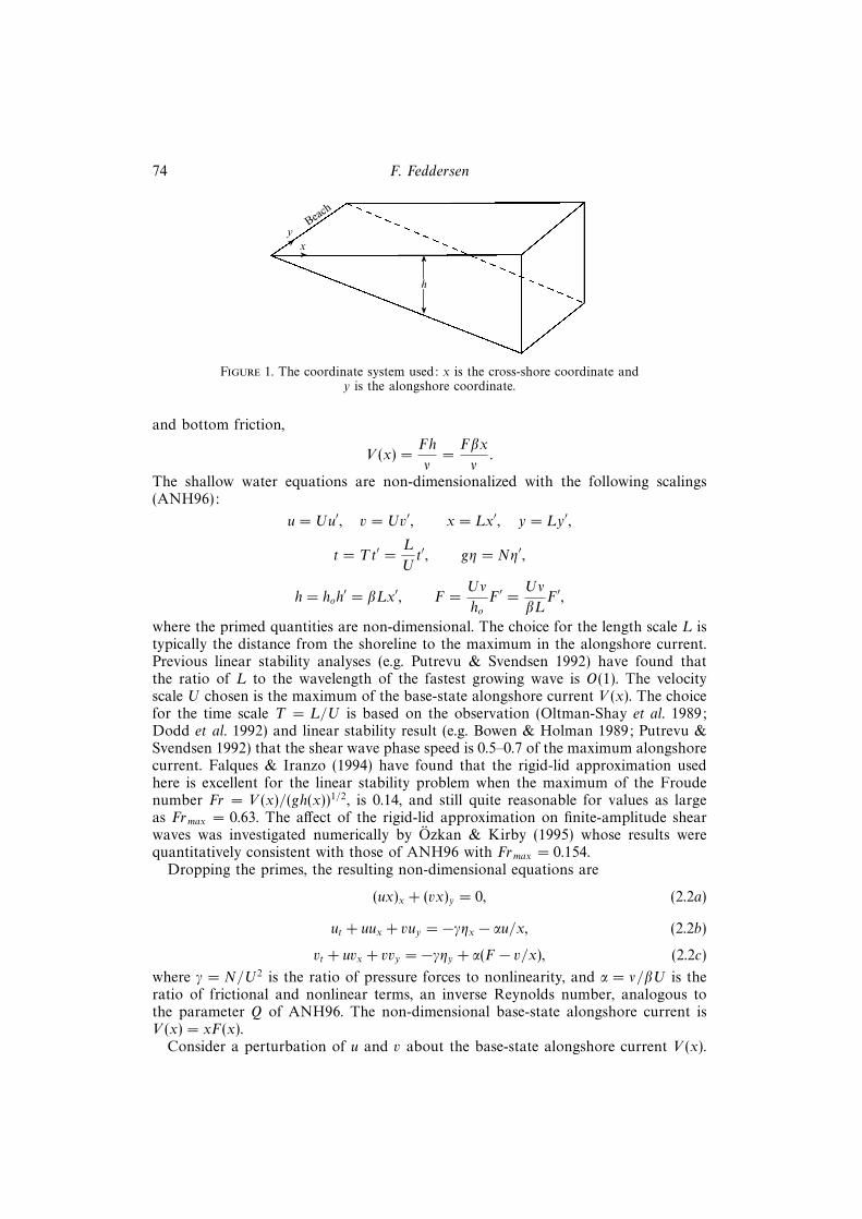
where x and y are the cross- and alongshore coordinates respectively (figure 1), uand v are the cross- and alongshore velocities, η is the sea surface elevation, ν is aconstant friction coefficient, and g represents gravity. This system of equations (2.1)is the same as in ANH96 except that biharmonic friction terms included in ANH96to dampen numerical instabilities are not required here. The bathymetry contours areplanar (h(x) = βx) and the shoreline is at x = 0. Following ANH96, the forcing F(x)from breaking, obliquely incident, surface-gravity waves is for simplicity alongshoredirected and does not vary in the alongshore direction. The bottom stress terms(e.g. νv/h) are an idealized representation of the bulk effects of bottom stress in thesurf zone. This representation has the advantage that it is simple analytically, andhas been used in the linear stability problem (Dodd et al. 1992; Falques & Iranzo1994) and by ANH96. Although other bottom stress representations which takeorbital wave velocities into account are probably more realistic in the surf zone (e.g.Thornton & Guza 1986), the simple bottom stress representation is appropriate forboth numerical-model-based (e.g. ANH96) and theory-based process studies of shearwaves, and allows comparison of the present results to ANH96.
If the alongshore current is steady and independent of y (i.e. v = V (x)), it thenfollows from the continuity equation and the boundary condition of no mass flux intothe shoreline (hu = 0 at x = 0) that u vanishes everywhere. The base-state alongshorecurrent whose stability will be investigated is then given by a balance between forcing
74 F. Feddersen
h
xy
Beach
Figure 1. The coordinate system used: x is the cross-shore coordinate andy is the alongshore coordinate.
and bottom friction,
V (x) =Fh
ν=Fβx
ν.
The shallow water equations are non-dimensionalized with the following scalings(ANH96):
u = Uu′, v = Uv′, x = Lx′, y = Ly′,
t = Tt′ =L
Ut′, gη = Nη′,
h = hoh′ = βLx′, F =
Uν
hoF ′ =
Uν
βLF ′,
where the primed quantities are non-dimensional. The choice for the length scale L istypically the distance from the shoreline to the maximum in the alongshore current.Previous linear stability analyses (e.g. Putrevu & Svendsen 1992) have found thatthe ratio of L to the wavelength of the fastest growing wave is O(1). The velocityscale U chosen is the maximum of the base-state alongshore current V (x). The choicefor the time scale T = L/U is based on the observation (Oltman-Shay et al. 1989;Dodd et al. 1992) and linear stability result (e.g. Bowen & Holman 1989; Putrevu &Svendsen 1992) that the shear wave phase speed is 0.5–0.7 of the maximum alongshorecurrent. Falques & Iranzo (1994) have found that the rigid-lid approximation usedhere is excellent for the linear stability problem when the maximum of the Froudenumber Fr = V (x)/(gh(x))1/2, is 0.14, and still quite reasonable for values as largeas Frmax = 0.63. The affect of the rigid-lid approximation on finite-amplitude shearwaves was investigated numerically by Ozkan & Kirby (1995) whose results werequantitatively consistent with those of ANH96 with Frmax = 0.154.
Dropping the primes, the resulting non-dimensional equations are
(ux)x + (vx)y = 0, (2.2a)
ut + uux + vuy = −γηx − αu/x, (2.2b)
vt + uvx + vvy = −γηy + α(F − v/x), (2.2c)
where γ = N/U2 is the ratio of pressure forces to nonlinearity, and α = ν/βU is theratio of frictional and nonlinear terms, an inverse Reynolds number, analogous tothe parameter Q of ANH96. The non-dimensional base-state alongshore current isV (x) = xF(x).
Consider a perturbation of u and v about the base-state alongshore current V (x).

Weakly nonlinear shear waves 75
The non-dimensional perturbation equations become
(ux)x + (vx)y = 0,
ut + uux + (v + V )uy = −γηx − αu/x,
vt + u(vx + Vx) + (v + V )vy = −γηy − αv/x.Taking the curl of the perturbation momentum equations, dividing by the waterdepth and substituting the continuity equation yields a perturbation potential vorticityequation
Dq
Dt+ uQx =
α
x
[−( vx
)x
+(ux
)y
],
whereD
Dt=
∂
∂t+ u
∂
∂x+ (V + v)
∂
∂y.
The perturbation potential vorticity is q = ζ/x, the perturbation vorticity is ζ = vx−uy ,and the background potential vorticity is Q = Vx/x. In terms of the perturbationtransport streamfunction ψ, where ψx = xv and ψy = −xu, the potential vorticitybecomes
q =1
x2
(∇2ψ − ψx/x
),
and the potential vorticity equation is
D
Dt
[1
x2(∇2ψ − ψx/x)
]− ψy
xQx = − α
x3
(∇2ψ − 2ψx/x
). (2.3)
The boundary conditions of no cross-shore mass flux at both the shoreline and faroffshore make ψ constant at x = 0 and ∞. The perturbation is assumed not to induceany net alongshore transport so ψ is the same constant (set for convenience to ψ = 0)at x = 0 and ∞. Fully expanded in terms of ψ and multiplied by x2, (2.3) becomes
(∇2ψ − ψx/x)t −ψy
x
(∇2ψx − 2∇2ψ/x− ψxx/x+ 3ψx/x
2)− xQxψy
+(V +
ψx
x
)(∇2ψy − ψxy/x) = −α
x
(∇2ψ − 2ψx/x
). (2.4)
This equation and the boundary conditions on ψ govern the evolution of shearinstabilities on a planar sloping bottom with a given base-state alongshore current.Substituting a perturbation expansion of ψ,
ψ = εψ1 + ε2ψ2 + ε3ψ3 + · · · , (2.5)
into (2.4) and collecting terms of O(ε) yields
L[ψ1] = (∇2ψ1 − ψ1x/x)t − xQxψ1y + V (∇2ψ1y − ψ1xy/x) +α
x
(∇2ψ1 − 2ψ1x/x
)= 0. (2.6)
This equation determines the linear stability of the flow. An alongshore propagatingwave solution for ψ1,
ψ1 = φ1(x) exp[ik(y − ct)] + c.c.,
is substituted into (2.6) where k is an alongshore wavenumber and c.c. denotes thecomplex conjugate. In general, c is complex. The real part cr is the phase speed and

76 F. Feddersen
is related to the frequency of the wave by ω = kcr . The imaginary part ci is relatedto the linear growth rate of the wave as σ = kci. Collecting terms proportional toexp[ik(y − ct)] yields (Dodd et al. 1992; ANH96)(
V − iα
kx− c)
(φ1xx − φ1x/x− k2φ1) = xQxφ1 −iα
kx2φ1x (2.7)
with boundary conditions φ1(0) = φ1(∞) = 0. For a particular paired value of k andα, an infinite set of paired eigenvalues c and eigenfunctions φ1(x) are solutions of(2.7). To proceed with the weakly nonlinear analysis, the critical α = αc is soughtsuch that there is only one wavenumber, k = kc, for which a single eigenvalueis purely real, while all others have negative imaginary parts. At all other wave-numbers the solutions decay (ci < 0). At (αc, kc), φ1(x) represents the single neutralmode corresponding to the critical eigenvalue. A dispersion relation is defined atαc:
ωc(k) + iσc(k) = kc, (2.8)
where c is the critical eigenvalue. A few properties of this dispersion relation are
σc(kc) = 0,∂ωc(kc)
∂k= cg,
∂σc(kc)
∂k= 0, (2.9)
where cg is the group velocity. After finding αc and kc, the finite-amplitude shearwave behaviour for small values of ε is found by setting α = αc(1 − ε2) so that theperturbation grows slowly. The evolution of the instability is determined at O(ε2) andO(ε3).
At O(ε2), the following scalings are introduced (Stewartson & Stuart 1971; Craik1985):
τ = ε2t, Y = ε(y − cgt), (2.10)
where τ is a slow time, and Y is a stretched alongshore coordinate moving with thegroup velocity, cg . The differential operators for time and the alongshore coordinateare replaced by
∂t → ∂t − εcg∂Y + ε2∂τ, ∂y → ∂y + ε∂Y . (2.11)
Again the perturbation streamfunction ψ is expanded in powers of ε (2.5), and ψ1,ψ2, and ψ3 have the following forms:
ψ1 = A(τ, Y )φ1(x) exp[ikc(y − ct)] + c.c., (2.12)
ψ2 = AA∗φ(0)2 (x)+AY φ
(1)2 (x) exp(ikc(y−ct))+A2φ
(2)2 (x) exp[2ikc(y−ct)]+c.c., (2.13)
ψ3 = |A|2Aφ(1)3 (x) exp[ikc(y − ct)] + c.c.+ · · · , (2.14)
where kc is the critical wavenumber, c is the phase speed of the neutral wave at (αc,kc), and A(τ, Y ) is the amplitude of the shear wave which may have slow variations inthe alongshore direction and in time. The term proportional to φ(0)
2 (x) represents the
correction to the mean transport, and that proportional to φ(2)2 (x) the forced harmonic
at twice the primary frequency (second harmonic).Applying the scalings for time and alongshore coordinate (2.11) to the full per-
turbation equation (2.4) with α = αc(1 − ε2) and collecting terms of O(ε) and O(ε2)gives
Lc[ψ1] = 0,

Weakly nonlinear shear waves 77
and
Lc[ψ2] =ψ1y
x
(∇2ψ1x − 2∇2ψ1/x− ψ1xx/x+ 3ψ1x/x
2)
−ψ1x
x
(∇2ψ1y − ψ1xy/x
)+ cg(∇2ψ1 − ψ1x/x)Y
−V (ψ1xx + 3ψ1yy − ψ1x/x)Y + xQxψ1Y − 2ψ1yY t −2αcxψ1yY , (2.15)
where the linear operator Lc[ψ] is the operator L[ψ] defined in (2.6) with α = αc.Substituting (2.12) for ψ1 and (2.13) for ψ2 into (2.15) and collecting terms proportionalto AA∗ yields
L0[φ(0)2 ] =
αc
x
(φ
(0)2xx −
2φ(0)2x
x
)=
ikcx
(φ1φ
∗1xxx − φ1xxxφ
∗1 + φ1xφ
∗1xx − φ1xxφ
∗1x
)+
3ikcx2
(φ1xxφ
∗1 − φ1φ
∗1xx
)+
3ikcx3
(φ1φ
∗1x − φ1xφ
∗1
)(2.16)
with the boundary conditions φ(0)2 = 0 at x = 0 and x = ∞. The linear operator L0 is
Ln (with n = 0), where
Ln[φ] = inkc
(V − iαc
nkcx− c)
(φxx − φx/x− (nkc)2φ)− inkcxQxφ−
αc
x2φx (2.17)
and n is an integer. The O(ε2) terms proportional to AY exp[ikc(y − ct)] give
L1[φ(1)2 ] = cg(φ1xx − φ1x/x− k2
cφ1)− V (φ1xx − φ1x/x− 3k2cφ1)
+
(xQx − 2k2
c c−2αcikcx
)φ1. (2.18)
In general, φ(1)2 is resonantly forced since the homogeneous problem, L1[ϕ] = 0, is
satisfied with the stated choice of αc, kc, and c. The solvability condition for φ(1)2
requires that cg satisfy
cg
∫ ∞0
φ†1(φ1xx − φ1x/x− k2
cφ1)dx =
∫ ∞0
φ†1V (φ1xx − φ1x/x− 3k2
cφ1)dx
−∫ ∞
0
φ†1
(xQx − 2k2
c c−2αcikcx
)φ1dx, (2.19)
where φ†1(x) is the adjoint function of φ1(x) and is defined in Appendix A. The cgfound by (2.19) should be equal to that found from the dispersion relationship (2.9),providing a useful check of both the algebra and the numerical computations. Withcg (2.18) can be solved for φ(1)
2 subject to boundary conditions φ(1)2 (x) = 0 at x = 0
and x = ∞. The O(ε2) terms proportional to A2 exp[2ikc(y − ct)] are
L2[φ(2)2 ] =
ikcx
(φ1φxxx − φ1xφ1xx) +ikcx2
(−3φ1φ1xx + 2k2
cφ21 + φ2
1x
)+
3ikcx3
(φ1φ1x) ,
(2.20)
where L2 is the operator Ln in (2.17) with n = 2. With the boundary conditions,φ
(2)2 = 0 at x = 0 and x = ∞, (2.18) can be solved for φ(2)
2 (x).The equation for the amplitude A(τ, Y ) of the instability is determined from O(ε3)

78 F. Feddersen
terms in (2.4) with α = αc(1− ε2),
L[ψ3] = −(∇2ψ1 −
ψ1x
x
)τ
+αc
x
(∇2ψ1 −
2ψ1x
x
)− αc
x(ψ1Y Y + 2ψ2yY )
−(ψ1Y Y t + 2ψ2yY t) + xQxψ2Y + cg
(2ψ1yY Y + ψ2xxY + ψ2yyY −
ψ2xY
x
)−V
(3ψ1yY Y + ψ2xxY + 3ψ2yyY −
ψ2xY
x
)+ψ1y
x
(∇2ψ2x −
3ψ2xx
x− 2ψ2yy
x+
3ψ2x
x2
)+ψ2y
x
(∇2ψ1x −
3ψ1xx
x− 2ψ1yy
x+
3ψ1x
x2
)+ψ1Y
x
(∇2ψ1x −
3ψ1xx
x− 2ψ1yy
x+
3ψ1x
x2
)+ψ1y
x
(2ψ1xyY −
4ψ1yY
x
)− ψ2x
x
(∇2ψ1y −
ψ1xy
x
)−ψ1x
x
(∇2ψ2y −
ψ2xy
x
)− ψ1x
x
(ψ1xxY + 3ψ1yyY −
ψ1xY
x
). (2.21)
The equation for A(τ, Y ) is derived by substituting (2.12) for ψ1 and (2.13) for ψ2,and invoking the solvability condition for ψ3. The terms on the right-hand side of(2.21) proportional to exp[ikc(y − ct)] are multiplied by the adjoint function φ
†1 and
integrated in the cross-shore direction. The left-hand side is identically zero (A 1) andsetting the right-hand side to zero yields a complex Ginzburg–Landau equation forthe amplitude of the instability
Aτ = σA+ δAY Y + µ|A|2A, (2.22)
where σ is the growth rate of the disturbance, δ is a dispersion term, and µ is theLandau coefficient which can limit the growth of the disturbance. These coefficientsare all complex in general. First κ, which is given by the terms proportional toAτ exp[ikc(y − ct)] on the right-hand side of (2.21), is defined
κ =
∫ ∞0
φ†1(φ1xx − φ1x/x− k2
cφ1) dx. (2.23)
The growth rate is given by the terms proportional to A exp[ikc(y − ct)] on theright-hand side of (2.21),
σ · κ =
∫ ∞0
φ†1
αc
x
(φ1xx − 2φ1x/x− k2
cφ1
)dx. (2.24)
The terms proportional to AY Y exp[ikc(y− ct)] on the right-hand side of (2.21) defineδ,
δ · κ =
∫ ∞0
φ†1Sdx, (2.25)
where
S =(−αcx
+ ikc(c+ 2cg − 3V ))φ1 +
(xQx − 2ikc
αc
x− k2
c (2c+ cg − 3V ))φ
(1)2
+V − cgx
φ(1)2x + (cg − V )φ(1)
2xx.

Weakly nonlinear shear waves 79
The terms on the right-hand side of the O(ε3) equation that are proportional to|A|2A exp[ikc(y − ct)] define the complex Landau constant µ,
µ · κ =
∫ ∞0
φ†1Tdx, (2.26)
where
T =ikcx
[2φ1φ
(0)2xxx − φ∗1φ
(2)2xxx − 2φ∗1xφ
(2)2xx + 2φ∗xxxφ
(2)2 − 2φ1xxφ
(0)2x + φ∗1xxφ
(2)2x
+k2c (3φ
∗1φ
(2)2x + 6φ∗1xφ
(2)2 + 2φ1φ
(0)2x )]
+ikcx2
(−6φ1φ
(0)2xx + 3φ∗1φ
(2)2xx + φ∗1xφ
(2)2x − 6φ∗1xxφ
(2)2 + 2φ1xφ
(0)2x − 4k2
cφ∗1φ
(2)2
)+
ikcx3
(6φ1φ
(0)2x − 3φ∗1φ
(2)2x + 6φ∗1xφ
(2)2
).
The complex Ginzburg–Landau equation (2.22) can exhibit a rich behaviour ofsolutions depending on the values of its coefficients (Manneville 1990). When the realpart of the Landau coefficient is negative, finite-amplitude solutions can be found ofthe form
A(τ, Y ) = B exp[i(ΛY − Ωτ)], (2.27)
where B is a complex constant. The simplest solution is when Λ = 0, and
|B|2 = −Re(σ)
Re(µ), (2.28)
Ω = −[Im(σ) + |B|2Im(µ)
]. (2.29)
This solution is side-band stable (Benjamin & Feir 1967; Stuart & DiPrima 1978) if
Im(µ)Im(δ)
Re(µ)Re(δ)+ 1 > 0. (2.30)
3. Calculations for ANH96 base-state conditionsThe beach slope (β = 0.05) and forcing of ANH96 will be used for the weakly
nonlinear calculations. The ANH96 base-state dimensional alongshore velocity is
V (x) = Cox2 exp
(−x
3
δ3
), (3.1)
where
Co = 2.404 609 9× 10⁻⁴ 1
m× s, δ = 103.02 m
so that the maximum in V is 1 m s−1 and occurs at x = 90 m. Therefore the chosenvelocity scale is U = 1 m s−1. The length scale becomes L = 90 m. The ratioL3/δ3 = 2/3, and the time scale is T = 90 s. The inverse Reynolds number for thesescaling choices is α = 20ν. The maximum Froude number is Frmax = 0.154, close tothe value of 0.14 found to satisfy the rigid-lid approximation for the linear stabilityproblem (Falques & Iranzo 1994). The non-dimensional base-state alongshore velocityV (x) and potential vorticity Q(x) become
V (x) = Vox2 exp
(−2x3/3
), Vo =
CoL2
U= exp(2/3), (3.2a)

80 F. Feddersen
1.0
0.8
0.6
0.4
0.2
0 1 2 3 4 5 6 7
4
3
2
1
0
0 1 2 3 4 5 6 7
–1
–2
x
Q (x)
V (x)
Figure 2. The base-state non-dimensional alongshore current V (x) (3.2a) and potentialvorticity Q(x) (3.2b).
Q(x) = 2Vo(1− x3) exp(−2x3/3
), (3.2b)
and are shown in figure 2. The potential vorticity has a minimum, which satisfies theRayleigh condition for inviscid instability.
ANH96 used a dimensional domain extending from x = 0 to x = 1000 m andfrom y = 0 to y = 450 m, corresponding to a non-dimensional domain extending tox = 11.111 and y = 5. Because the solution is expected to decay exponentially offshore(Appendix B) a smaller non-dimensional domain extending to x = 7.5 is used here. Asecond-order finite difference scheme is used with N−1 grid points so δx = 7.5/N. Inorder to accurately do the weakly nonlinear analysis, αc, kc, c, and the eigenfunctionsmust be precisely known. Therefore, c and φ1 are extrapolated from calculations inextended precision (32 significant digits) on grids with N − 1, 2N − 1, and 4N − 1points, giving an accuracy of O(δx6). To find αc and the dispersion relationship, (2.7)was solved on the three grids using N = 2500 (δx = 0.003) by inverse iteration,which is highly efficient for large tridiagonal systems (Golub & Van Loan 1996).From the solutions on the three grids, c and φ1 are extrapolated giving errors ofO(δx6) = 10−16. A search was performed in (α, k) space to find the pair of values(αc,kc) where one eigenvalue has a zero imaginary component, and all the others havenegative imaginary components. For the given beach slope and background velocity,the critical values are αc = 0.201 189 612 42 and kc = 1.363 262 549 16. The eigenvaluespectrum is shown in figure 3(a). The critical eigenvalue is well separated from theother eigenvalues (figure 3b). The adjoint eigenvalue spectrum at αc and kc from(A 2) is calculated in the same manner and, as expected, is identical to the eigenvaluespectrum of (2.7). The numerical value of the maximum non-dimensional growth rateat αc is very close to zero (σc(kc) = kcci = 2× 10⁻¹¹, corresponding to a dimensionalgrowth time scale of 105 years). The points on the dispersion relation (2.8) near kc arewell fitted by a parabola (figure 4, the coefficients of the parabola are given in table 1)indicating that a Taylor series expansion of the dispersion relationship near kc is

Weakly nonlinear shear waves 81
0.2
0
–0.2
–0.4
–0.6
–0.8
–1.00 0.2 0.4 0.6 0.8 1.0
(a)
cr
ci
0.005
0
–0.025
0 0.2 0.4 0.6 0.8 1.0
(b)
cr
–0.030
–0.020
–0.015
–0.010
–0.005
Figure 3. (a) Real and imaginary parts of the eigenvalues of (2.7) at αc = 0.201 189 andkc = 1.363 262 549, and (b) the spectrum enlarged to show the region −0.030 < ci < 0.005.
1.3628 1.3630 1.3632 1.3634 1.3636–2
–1
0
(× 10–8)
1
0.8424
0.8422
0.8420
1.3628 1.3630 1.3632 1.3634 1.3636
k
ωc(k)
σc(k)
Figure 4. The critical dispersion curve for ωc(k) + iσc(k) = kc near the critical wavenumber k. Thecircles represent calculated values. The solid lines are the best-fit parabolas from the coefficients oftable 1.
valid. Based on the coefficients in table 1, the phase speed at the critical wavenumberis c = 0.617 753 649 7 and by (2.9) the group velocity is cg = 0.490 600 164 4.
Once the critical frictional parameter and wavenumber are known, φ1 is calculatedfrom (2.7) using αc and kc with the same numerical scheme on much denser grids whereN = 10 000 (δx = 7.5 × 10⁻⁴). Denser grids are used because third derivatives mustbe accurately calculated to find the coefficients of the complex Ginzburg–Landau

82 F. Feddersen
a2 a1 a0
ω(k) 0.012 869 479 738 04 0.490 600 164 421 66 0.842 160 415 251 88σ(k) −0.088 322 793 143 48 0 1.893 23× 10−11
Table 1. The quadratic coefficients for the growth rate and frequency,ωc(k) + iσc(k) = a2(k − kc)2 + a1(k − kc) + a0 where kc = 1.363 262 549 16.
σ 0.123 746− i0.014 047δ 0.088 330 + i0.012 854µ −321.730 54 + i407.930 56|B| 0.0196 11Ω −0.1428 53
Table 2. Coefficients for the complex Ginzburg–Landau equation and solution values.
equation. The real and imaginary parts of the normalized and extrapolated φ1 areshown in figure 5(a). The adjoint function φ†1, shown in figure 5(b), is calculated in asimilar manner. The group velocity cg calculated from (2.19), where the derivatives ofφ1 and the integrals are extrapolated, yields a value of cg = 0.490 600 157 2− 0.35×10⁻⁸i. This agrees with the value from the dispersion relationship (2.9) to 10−8 in boththe real and imaginary parts, serving as a check of the numerical computations. Thefunctions φ(0)
2 and φ(2)2 (figure 5c and figure 5e) are calculated from (2.16) and (2.20)
on grids identical to those used for φ1 with a standard tridiagonal matrix solver,and extrapolated. The function φ
(1)2 is found by solving (2.18) with a singular value
decomposition of the L1 matrix with N = 999 grid points. There is one well-isolatedzero (10−13) singular value, and the forward and adjoint null vectors of the L1 matrixare proportional to φ1 and φ
†1. The solution for φ(1)
2 (figure 5d) is constructed by
suppressing the homogeneous solution to L1. The derivatives of φ1, φ(0)2 , φ(1)
2 , φ(2)2
and the integrals in (2.23), (2.24), (2.26) are extrapolated to derive the coefficientsof the complex Ginzburg–Landau equation (2.22), summarized in table 2. The valueof δ can also be calculated (Stewartson & Stuart 1971) from the linear dispersionrelationship (figure 4 and the dispersion relation coefficients in table 1) by
δ = −1
2
∂2σc
∂k2+ i
1
2
∂2ωc
∂k2. (3.3)
These two estimates of δ agree to three significant digits. The accuracy of theagreement between the two is much smaller than that between the two estimates ofcg (from (2.9) and (2.19)), because δ is calculated from (2.25) where φ(1)
2 (x) is foundon a much coarser grid than for example φ1(x).
The real part of the Landau coefficient is negative so in this case the instabilityis supercritical, and finite-amplitude equilibration is possible. A solution for theamplitude of the shear wave is sought that has the form (2.27) with Λ = 0. The valuesof B (2.28) and Ω (2.29) are given in table 2. The values of µ and δ are such thatthis solution for A(τ, Y ) is side-band stable (2.30) for the stated choice of beach slopeand base-state alongshore current. For other choices of beach slope and base-statealongshore currents, the instability could be either subcritical or side-band unstable.

Weakly nonlinear shear waves 83
(a)
(b)
(c)
(d)
(e)
76543210–5
0
5
10
–0.5
0
0.5
–20
–10
0
10
–1
0
1
–0.5
0
0.5
1.0
φ(2)2
φ(1)2
φ(0)2
φ†2
φ1
x
Figure 5. The real (solid) and imaginary (dashed) parts of (a) φ1, (b) φ†1, (c) φ(0)2 ,
(d) φ(1)2 , and (e) φ(2)
2 .
4. Analytic and numerical model comparisonDue to numerical limitations, the near critical behaviour of the ANH96 model may
be distorted. Therefore, analytic and ANH96 numerical results will be compared forthe same non-dimensional beach profile (h = x) and base-state alongshore current(3.2a) at two values of α = 0.18 and 0.17. There are differences between the twomodels. The ANH96 model is a second-order finite-difference model of essentiallythe equations (2.1), but also includes weak biharmonic friction (−ν∗∇4u and −ν∗∇4vadded to the right-hand side of (2.1b) and (2.1c)) to suppress numerical instabilities.Boundary conditions of no flow into the shoreline and offshore boundary are used.Additional boundary conditions (uxx = vx = vxxx = 0) are required at the shorelineand offshore boundary in the ANH96 model due to the fourth-order derivativesin the biharmonic friction terms. The finite-difference representation for biharmonicfriction and the associated boundary conditions may influence the development ofthe instability. ANH96 use a numerical resolution with N = 200 grid points in x,M = 90 points in y, and a non-dimensional grid spacing δx = δy = 0.044. The

84 F. Feddersen
0.1 0.2 0.30
2
4
6
8
(a)
ε
Pri
mar
y am
plit
ude
(× 10–3)
0.05 0.100
0.5
1.0
1.5
2.0
(b)
ε2
2nd
harm
onic
am
plitu
de
(× 10–3)2.5
Figure 6. (a) The ANH96 model peak amplitude at the primary frequency at x = 1 versus ε forα = 0.18 (∗) and α = 0.17 (). The inferred αc = 0.185 64. (b) The amplitude of the second harmonicversus ε2. The inferred αc = 0.187 41.
finite numerical resolution of ANH96 may also mask the near critical behaviour (e.g.Hyman et al. 1986).
Periodic boundary conditions are used in the alongshore direction, and the along-shore domain is slightly longer than the wavelength of the theoretical critical wave,leading to a smaller wavenumber (k = 1.2566 vs. kc = 1.3632) for the ANH96 criticalwave. Therefore the most unstable wave cannot grow, and an evolution of the insta-bility to smaller wavenumbers is restricted. ANH96 also ran numerical experimentswith an alongshore domain three times the wavelength of the most unstable modeand stronger nonlinearity (α 6 0.12 corresponding to ε > 0.6), and reported a shifttoward lower frequencies and wavenumbers as the instability evolved. For α = 0.15(ε ≈ 0.45), more strongly nonlinear than the values of α investigated here, steadyequilibrated waves with the same frequencies and wavenumber as the experimentswith the smaller domains were reported (figure 7 of ANH96). However, even onthe extended alongshore domain, a potential side-band instability of the shear waveis still suppressed. Due to these limitations of the ANH96 model, the near criticalbehaviour of shear waves may be modelled incorrectly, and for these reasons, the αcand hence ε for the ANH96 model are not accurately known.
Before comparing the results of the ANH96 model with the analytic model, itis first verified that the ANH96 model at αc = 0.17 and αc = 0.18 is in a weaklynonlinear regime. For weakly nonlinear waves, the amplitude at the primary frequencya1 depends linearly on ε and the amplitude at the second harmonic a2 depends onε2. Both amplitudes should vanish when ε = 0. The αc is found so that the line goingthrough the (ε,a1) and (ε2,a2) points have zero y-intercept (figure 6). The resultingestimates of αc are quite similar, αc = 0.185 64 from the primary frequency andαc = 0.18741 from the second harmonic, confirming the ANH96 model is in a weaklynonlinear regime. Using αc = 0.185 64, ε = 0.174 for α = 0.18 and ε = 0.290 forα = 0.17.
The choice of αc feeds back into all parts of the solution to the weakly nonlinearproblem, so it is not possible to use the ANH96-derived αc to compare results fromthe ANH96 and analytic models. Therefore, the analytic αc = 0.20119 is used tocalculate ε for comparison purposes, resulting in ε = 0.325 for α = 0.18 and ε = 0.394for α = 0.17. As will be shown, this leads to reasonable agreement between analyticand ANH96 model amplitudes for the shear waves, and very good agreement for thecross-shore structure of the shear waves.
The spectrum of ANH96 cross-shore velocity at both values of α contains distinct

Weakly nonlinear shear waves 85
10–18
10–16
10–14
10–12
10–10
10–8
10–6
10–4
10–2
100
0 0.5 1.5 2.0 2.5 3.0 3.5 4.01.0
Non-dimensional radian frequency
Figure 7. Non-dimensional spectra of u at x = 1 from ANH96 model with α = 0.17 (grey line)and 0.18 (bold line).
peaks at integer multiples of the primary frequency (figure 7). The primary peak inthe spectrum at the weakest nonlinearity (α = 0.18) has a dimensional period of 12minutes. The ANH96 model non-dimensional primary frequency ω1 = 0.7822 is closeto the analytical model value ω = 0.8421 at αc and kc from linear stability theory(2.7). The difference in frequencies is largely attributable to the ANH96 alongshoredomain being slightly longer than the critical wavelength. From (2.7), the smallerwavenumber forced by the domain size corresponds to a frequency ω = 0.7899, closeto the ANH96 primary frequency ω1 = 0.7822.
The shift to lower frequency in the spectral peaks with decreasing α (figure 7)is consistent with amplitude dispersion. The equilibrated cross-shore velocity at theprimary frequency and at a fixed alongshore position is
u =−εikx
(Bφ1(x)e−i(ωc+ε
2Ω)t − B∗φ∗1(x)ei(ωc+ε2Ω)t)
(4.1)
indicating a finite-amplitude shift of ε2Ω in the primary frequency, where Ω is givenby (2.29). At the nth harmonic (e.g. nω1) the leading-order frequency shift is given bynε2Ω. Therefore the difference in spectral peak frequencies at α = 0.18 and α = 0.17is theoretically n∆ε2Ω, where ∆ε2 = (0.18− 0.17)/αc. The ANH96 observed frequencyshift for the first four harmonics at the nth harmonic is n times the primary frequencyshift (figure 8), consistent with O(ε2) amplitude dispersion. However, the magnitudeof the ANH96 observed frequency shift is about 30% larger than the analytical modelfrequency shift.
The equilibrated cross-shore velocity of the ANH96 model at a fixed alongshore

86 F. Feddersen
0.04
0.03
0.02
0.01
0 0.01 0.02 0.03 0.04
Theory Dω
Obs
erve
d D
ω
Figure 8. The ANH96-derived versus the theoretical change in peak frequency between α = 0.18and α = 0.17. Results for the primary frequency (∗), second (), third (), and fourth (4) harmonicare shown with αc = 0.201 19. The error bars (±0.003) indicate the frequency resolution of thespectrum. The solid line represents perfect ANH96 model–theory agreement. The dashed line is thebest fit through the symbols.
position is
u(x, t) = U1(x)eiω1t +U2(x)ei2ω1t + c.c.+ · · · , (4.2)
where ω1 is the primary wave frequency, and U1(x) and U2(x) are the Fouriertransforms of the ANH96 cross-shore velocities at ω1 and 2ω1. U1(x) and U2(x) arerelated to the analytic model by
U1(x) =−εB∗ikφ∗1(x)
xU2(x) =
−ε2B∗22ikφ(2)∗2 (x)
x. (4.3a,b)
The functions φ1(x) and φ(2)2 (x) can therefore be inferred from the ANH96 cross-
shore velocity for α = 0.18 and α = 0.17. The magnitudes of |φ1(x)| and |φ(2)2 (x)| are
equal to the square root of the spectrum of u (e.g. figure 7) summed over a smallwindow of frequencies centred on the primary or secondary frequency (to account forspectral leakage) and multiplied by x/(ε|B|k) or x/(2ε2|B|2k) respectively. The phases
of φ1(x) and φ(2)2 (x) are given within arbitrary constants from the phases of U1(x) or
U2(x).
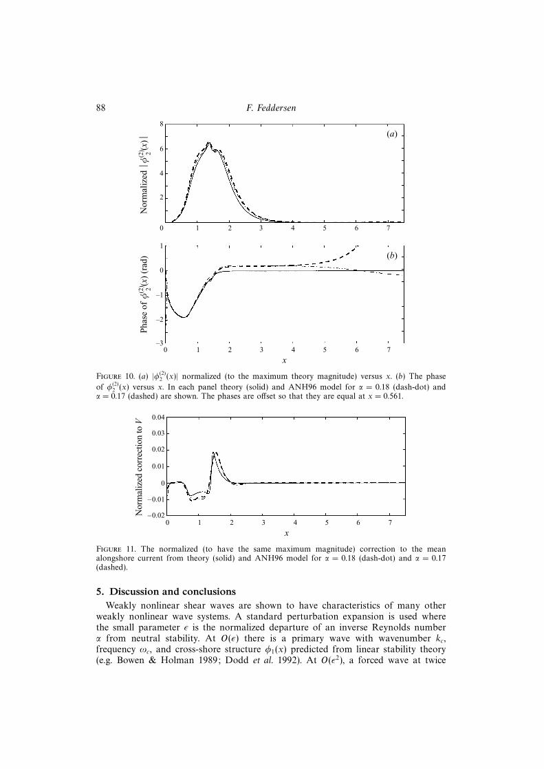
Analytic and ANH96 model solutions for φ1(x) and for φ(2)2 (x) are shown in
figures 9 and 10. The magnitudes of the ANH96-derived φ1(x) are in approximateagreement with theory (figure 9a) using the ε derived from the analytic αc. However,when normalized to the same maximum magnitude, the cross-shore structure of boththe ANH96-inferred and theoretical |φ1(x)| and |φ(2)
2 (x)| are in very good agreementfor both values of α (figures 9b and 10a). The cross-shore phase structure is also inexcellent agreement (figure 9c and figure 10b), except near the shoreline where thedifferences are evidently due to the additional boundary conditions applied to theANH96 model at the shoreline and the resulting boundary layer from the biharmonicfriction. Far offshore (x > 4), the phase for φ(2)
2 (x) is in error because the signal is soweak.

Weakly nonlinear shear waves 87
2.0
1.5
1.0
0.5
0 1 2 3 4 5 6 7
(a);
φ1(x
);
1.0
0.8
0.6
0.4
0 1 2 3 4 5 6 7
(b)
Nor
mal
ized
;φ
1(x
);
0.2
1
0
–1
–2
0 1 2 3 4 5 6 7
(c)
Pha
se o
f φ
1(x
) (r
ad)
–3
xFigure 9. (a) |φ1(x)| versus non-dimensional cross-shore coordinate, x. (b) |φ1(x)| normalized (to amaximum magnitude of 1.0) versus x. (c) The phase of φ1(x) versus x. In each panel, theory is asolid line, and ANH96 model φ1(x) are inferred with αc = 0.20119, and are shown with α = 0.18(dash-dot) and α = 0.17 (dashed). The phases are offset so that they are equal at x = 0.582.
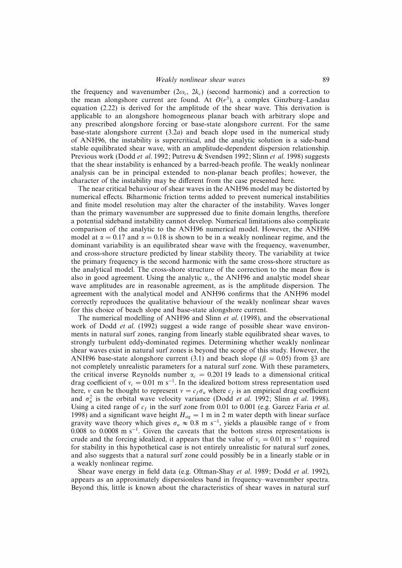
The analytic model predicts a mean second-order correction Vc(x) to the alongshorecurrent
Vc(x) =ε2|B|2φ(0)
2x
x. (4.4)
The ANH96 correction, defined as the difference between the time mean from thebase-state alongshore current v(x)−V (x), was calculated for both α. The ε2-normalizedtheoretical correction to the alongshore current, Vc/ε
2 = |B|2φ(0)2x/x, and the ANH96
correction (v − V )/ε2 normalized to the same magnitude are also in very goodagreement (figure 11). The differences in the correction near the shoreline are againdue to the additional boundary conditions applied there. The effect of the mean flowcorrection is to reduce the offshore velocity shear by decreasing the velocity at themaximum near x = 1 and increasing the velocity further offshore.
88 F. Feddersen
8
6
4
0 1 2 3 4 5 6 7
(a)N
orm
aliz
ed;
φ(2
) 2 (x
);
2
1
0
–1
–2
0 1 2 3 4 5 6 7
(b)
Pha
se o
f φ
(2) 2 (x
) (r
ad)
–3
x
Figure 10. (a) |φ(2)2 (x)| normalized (to the maximum theory magnitude) versus x. (b) The phase
of φ(2)2 (x) versus x. In each panel theory (solid) and ANH96 model for α = 0.18 (dash-dot) and
α = 0.17 (dashed) are shown. The phases are offset so that they are equal at x = 0.561.
0.04
0.02
0.01
0 1 2 3 4 5 6 7
Nor
mal
ized
cor
rect
ion
to V
–0.02
x
–0.01
0
0.03
Figure 11. The normalized (to have the same maximum magnitude) correction to the meanalongshore current from theory (solid) and ANH96 model for α = 0.18 (dash-dot) and α = 0.17(dashed).
5. Discussion and conclusionsWeakly nonlinear shear waves are shown to have characteristics of many other
weakly nonlinear wave systems. A standard perturbation expansion is used wherethe small parameter ε is the normalized departure of an inverse Reynolds numberα from neutral stability. At O(ε) there is a primary wave with wavenumber kc,frequency ωc, and cross-shore structure φ1(x) predicted from linear stability theory(e.g. Bowen & Holman 1989; Dodd et al. 1992). At O(ε2), a forced wave at twice
Weakly nonlinear shear waves 89
the frequency and wavenumber (2ωc, 2kc) (second harmonic) and a correction tothe mean alongshore current are found. At O(ε3), a complex Ginzburg–Landauequation (2.22) is derived for the amplitude of the shear wave. This derivation isapplicable to an alongshore homogeneous planar beach with arbitrary slope andany prescribed alongshore forcing or base-state alongshore current. For the samebase-state alongshore current (3.2a) and beach slope used in the numerical studyof ANH96, the instability is supercritical, and the analytic solution is a side-bandstable equilibrated shear wave, with an amplitude-dependent dispersion relationship.Previous work (Dodd et al. 1992; Putrevu & Svendsen 1992; Slinn et al. 1998) suggeststhat the shear instability is enhanced by a barred-beach profile. The weakly nonlinearanalysis can be in principal extended to non-planar beach profiles; however, thecharacter of the instability may be different from the case presented here.
The near critical behaviour of shear waves in the ANH96 model may be distorted bynumerical effects. Biharmonic friction terms added to prevent numerical instabilitiesand finite model resolution may alter the character of the instability. Waves longerthan the primary wavenumber are suppressed due to finite domain lengths, thereforea potential sideband instability cannot develop. Numerical limitations also complicatecomparison of the analytic to the ANH96 numerical model. However, the ANH96model at α = 0.17 and α = 0.18 is shown to be in a weakly nonlinear regime, and thedominant variability is an equilibrated shear wave with the frequency, wavenumber,and cross-shore structure predicted by linear stability theory. The variability at twicethe primary frequency is the second harmonic with the same cross-shore structure asthe analytical model. The cross-shore structure of the correction to the mean flow isalso in good agreement. Using the analytic αc, the ANH96 and analytic model shearwave amplitudes are in reasonable agreement, as is the amplitude dispersion. Theagreement with the analytical model and ANH96 confirms that the ANH96 modelcorrectly reproduces the qualitative behaviour of the weakly nonlinear shear wavesfor this choice of beach slope and base-state alongshore current.
The numerical modelling of ANH96 and Slinn et al. (1998), and the observationalwork of Dodd et al. (1992) suggest a wide range of possible shear wave environ-ments in natural surf zones, ranging from linearly stable equilibrated shear waves, tostrongly turbulent eddy-dominated regimes. Determining whether weakly nonlinearshear waves exist in natural surf zones is beyond the scope of this study. However, theANH96 base-state alongshore current (3.1) and beach slope (β = 0.05) from §3 arenot completely unrealistic parameters for a natural surf zone. With these parameters,the critical inverse Reynolds number αc = 0.201 19 leads to a dimensional criticaldrag coefficient of νc = 0.01 m s−1. In the idealized bottom stress representation usedhere, ν can be thought to represent ν = cfσu where cf is an empirical drag coefficientand σ2
u is the orbital wave velocity variance (Dodd et al. 1992; Slinn et al. 1998).Using a cited range of cf in the surf zone from 0.01 to 0.001 (e.g. Garcez Faria et al.1998) and a significant wave height Hsig = 1 m in 2 m water depth with linear surfacegravity wave theory which gives σu ≈ 0.8 m s−1, yields a plausible range of ν from0.008 to 0.0008 m s−1. Given the caveats that the bottom stress representations iscrude and the forcing idealized, it appears that the value of νc = 0.01 m s−1 requiredfor stability in this hypothetical case is not entirely unrealistic for natural surf zones,and also suggests that a natural surf zone could possibly be in a linearly stable or ina weakly nonlinear regime.
Shear wave energy in field data (e.g. Oltman-Shay et al. 1989; Dodd et al. 1992),appears as an approximately dispersionless band in frequency–wavenumber spectra.Beyond this, little is known about the characteristics of shear waves in natural surf

90 F. Feddersen
zones. Future analyses and observations may better characterize surf zone shear waveenvironments. If shear waves are weakly nonlinear equilibrated linear modes, thismight be elucidated with bispectral analysis (e.g. Elgar & Guza 1985) because in theweakly nonlinear limit, the wave at 2ω and 2k is bound to the primary wave at ωand k. Future theoretical and observational study could include investigating possibleresonances between modes, either leading to explosive instabilities (Shrira et al. 1997)or a coupled set of amplitude equations.
Funding for this study was provided by ONR Coastal Sciences and AASert pro-grams, and California Sea Grant. The author appreciates the help of by John Allenand Priscilla Newberger in providing ouput from their model. Glenn Ierley and BobGuza provided sage advice on many occasions, and Paola Cessi taught the class thatinspired this work.
Appendix A. The adjoint operator
The adjoint operator, L†1 and the adjoint function φ†1 to the linear operator L1 aredefined as ∫ ∞
0
φ†1L1[φ1]dx =
∫ ∞0
φ1L†1[φ
†1]dx = 0 (A 1)
with L1[φ1] given by (2.17) with n = 1 and and the boundary conditions, φ1 = 0 atx = 0 and x = ∞. Integrating by parts yields
L†[φ†1] =
(V − iαc
kcx− c)φ†1xx +
(2Vx +
V
x− c
x
)φ†1x −
(xQx −
iαckcx
(k2c +
2
x2
)+V
(k2c +
1
x2
)− Vx
x− Vxx − c
(k2c +
1
x2
))φ†1 = 0, (A 2)
with the boundary conditions φ†1 = 0 at x = 0 and ∞. The adjoint φ†1 is solved at thecritical wavenumber, kc and critical friction parameter, αc. The adjoint operator L†
must and does have the same eigenvalue spectrum as the linear operator L1.
Appendix B. AsymptoticsThe asymptotic nature of the linear eigenvalue problem near the beach (x = 0)
is examined where the dimensional water depth, h → 0. The solution of the lineareigenvalue problem should be analytic near the shoreline and match the prescribedboundary condition, φ1 = 0. The non-dimensional velocity used by ANH96 (3.2a)and resulting potential vorticity gradient are expanded around x = 0. The stabilityequation (2.7) is rewritten as
φ1xx −φ1x
x− k2φ1 =
(Qox
3φ1 − iαkx2φ1x
)(Vox
2 − c+ iαkx
)(Vox
2 − c− iα
kx
)(Vox
2 − c+iα
kx
)= λ1(x)φ1 + iλ2(x)φ1x + φ1x/x,
where λ1(x) and λ2(x) are analytic functions near x = 0. The origin is a regularsingular point. Expanding in a Frobenius series, the indicial exponents are 0 and3. The latter gives a non-singular solution that satisfies the boundary condition,φ1(0) = 0.
The asymptotic behaviour as x → ∞ is also of interest because the solution for

Weakly nonlinear shear waves 91
φ1 should match the boundary condition of φ1(∞) = 0, in checking the numericalsolution for φ1 and helping to choose the proper numerical domain. As x→∞, termsthat are proportional to V and Qx can be ignored since both have leading-orderbehaviour exp(−2x3/3). The equation becomes(
c+iα
kx
)φ1xx −
(c+
2iα
kx
)φ1x
x−(c+
iα
kx
)k2φ1 = 0,
which has an irregular singular point at x = ∞. Substituting φ1 = eS(x), standardasymptotic methods are used to determine that to leading order S ∼ −kx + 1/2 ln xthus
φ1 ∼ x1/2 exp(−kx).
Note that this leading order result is independent of both the eigenvalue c and α.
REFERENCES
Allen, J. S., Newberger P. A. & Holman R. A. 1996 Nonlinear shear instabilities of alongshorecurrents on plane beaches. J. Fluid Mech. 310, 181–213 (referred to herein as ANH96).
Benjamin, T. B. & Feir, J. E. 1967 The disintegration of wave trains on deep water. J. Fluid Mech.27, 417–430.
Bowen, A. J. & Holman, R. A. 1989 Shear instabilities of the mean longshore current, 1. Theory.J. Geophys. Res. 94, 18023–18030.
Craik, A. D. D. 1989 Wave Interactions and Fluid Flows. Cambridge University Press.
Dodd, N., Oltman-Shay, J. & Thornton, E. B. 1992 Shear instabilities in the longshore current: acomparison of observation and theory. J. Phys. Oceanogr. 22, 62–82.
Dodd, N. & Thornton, E. B. 1992 Longshore current instabilities: growth to finite amplitude. Proc.23rd Intl Conf. Coastal Engng, pp. 2644–2668. ASCE.
Elgar, S. & Guza, R. T. 1985 Observations of bispectra of shoaling surface gravity waves. J. FluidMech. 161, 425–448.
Falques, A. & Iranzo, V. 1994 Numerical simulation of vorticity waves in the nearshore. J. Geophys.Res. 99, 825–841.
Garcez Faria, A. F., Thornton, E. B., Stanton, T. P., Soares, C. M. & Lippmann, T. C. 1998Vertical profiles of longshore currents and related bed shear stress and bottom roughness. J.Geophys. Res. 103, 3217–3232.
Golub, G. H. & Van Loan, C. F. 1996 Matrix Computations, 3rd edn. Johns Hopkins UniversityPress.
Hyman, J. M., Nicolaenko, B. & Zaleski, S. 1986 Order and complexity in the Kuramoto-Sivashinsky model of weakly turbulent interfaces. Physica D 23, 265–292.
Manneville, P. 1990 Dissipative Structures and Weak Turbulence. Academic Press.
Oltman-Shay, J., Howd, P. A. & Birkemeier, W. A. 1989 Shear instabilities of the mean longshorecurrent, 2. Field data. J. Geophys. Res. 94, 18,031–18042.
Ozkan, H. T. & Kirby, J. T. 1995 Finite amplitude shear wave instabilities. Proc. Coastal Dynamics1995, pp. 465–476. ASCE.
Putrevu, U. & Svendsen, I. A. 1992 Shear instability of longshore currents: A numerical study. J.Geophys. Res. 97, 7283–7302.
Shrira, V. I., Voronovich, V. V. & Kozhelupova, N. G. 1997 Explosive instability of vorticitywaves. J. Phys. Oceanogr. 27, 542–554.
Slinn, D. N., Allen, J. S., Newberger, P. A. & Holman, R. A. 1998 Nonlinear shear instabilitiesof alongshore currents over barred beaches. J. Geophys. Res. (in press).
Stewartson, K. & Stuart, J. T. 1971 A non-linear instability theory for a wave system in planePoiseulle flow. J. Fluid Mech. 48, 529–545.
Stuart, J. T. & DiPrima, R. C. 1978 The Eckhaus and Benjamin-Feir resonance mechanisms. Proc.R. Soc. Lond. A 362, 27–41.
Thornton, E. B. & Guza, R. T. 1986 Surf zone longshore currents and random waves: field dataand models. J. Phys. Oceanogr. 16, 1165–1178.