WEAKLY IMPLICIT NUMERICAL SCHEMES - UiSsevje/files/1-60063.pdfThe aim of this paper is to construct semi-implicit numerical schemes for a two-phase (two-ﬂuid) ﬂow model, allowing

SIAM J. SCI. COMPUT. c© 2005 Society for Industrial and Applied MathematicsVol. 26, No. 5, pp. 1449–1484

WEAKLY IMPLICIT NUMERICAL SCHEMESFOR A TWO-FLUID MODEL∗

STEINAR EVJE† AND TORE FLATTEN‡

Abstract. The aim of this paper is to construct semi-implicit numerical schemes for a two-phase(two-fluid) flow model, allowing for violation of the CFL criterion for sonic waves while maintaininga high level of accuracy and stability on volume fraction waves.

By using an appropriate hybridization of a robust implicit flux and an upwind explicit flux,we obtain a class of first-order schemes, which we refer to as weakly implicit mixture flux (WIMF)methods. In particular, by using an advection upstream splitting method (AUSMD) type of upwindflux [S. Evje and T. Flatten, J. Comput. Phys., 192 (2003), pp. 175–210], we obtain a scheme denotedas WIMF-AUSMD.

We present several numerical simulations, all of them indicating that the CFL-stability of theWIMF-AUSMD scheme is governed by the velocity of the volume fraction waves and not the rapidsonic waves. Comparisons with an explicit Roe scheme indicate that the scheme presented in thispaper is highly efficient, robust, and accurate on slow transients. By exploiting the possibility to takemuch larger time steps, it outperforms the Roe scheme in the resolution of the volume fraction wavefor the classical water faucet problem. On the other hand, it is more diffusive on pressure waves.

Although conservation of positivity for the masses is not proved, we demonstrate that a fix maybe applied, making the scheme able to handle the transition to one-phase flow while maintaining ahigh level of accuracy on volume fraction fronts.

Key words. two-phase flow, two-fluid model, hyperbolic system of conservation laws, fluxsplitting, implicit scheme

AMS subject classifications. 76T10, 76N10, 65M12, 35L65

DOI. 10.1137/030600631

1. Introduction. This paper deals with numerical solutions to a classical four-equation two-fluid model for isentropic flows in one space dimension. The model wewill be concerned with (described in detail in section 2) is classified as a hyperbolicset of differential equations, with the implication that information flows in the systemalong characteristic curves with a certain velocity. For such models explicit numericalschemes are commonly used, advantage being taken of the fact that the time devel-opment of the state at some point depends only on points within the span of thecharacteristic curves in time and space. Explicit schemes are simple to implementand may give more flexibility in the treatment of complex pipe networks. However,they are subject to the CFL constraint

Δx

Δt≥ |λmax|,(1)

where λmax is the largest eigenvalue for the system. For the two-fluid model we areconcerned with, the four eigenvalues are pairwise associated with sonic and volumefraction waves [9]. The sonic waves may be several orders of magnitude faster thanthe volume fraction waves, although the latter may often be of greater interest to the

∗Received by the editors August 7, 2003; accepted for publication (in revised form) July 8, 2004;published electronically April 19, 2005.

http://www.siam.org/journals/sisc/26-5/60063.html†RF-Rogaland Research, Prof. Olav Hanssensvei 15, Stavanger, Norway ([email protected]).‡Department of Energy and Process Engineering, Norwegian University of Science and Technology,

Kolbjørn Hejes vei 1B, N-7491, Trondheim, Norway ([email protected]). This author wassupported in part by the Petronics program of the Norwegian Research Council.

1449

1450 STEINAR EVJE AND TORE FLATTEN

researcher. For this reason the CFL criterion (1) may severely limit the computationalefficiency of explicit schemes.

To remedy the situation, a step in a more implicit direction, i.e., coupling one ormore variables throughout the computational domain, may be made. Such approachesmay be classified as follows:

• Weakly implicit. The original CFL criterion (1) may be broken for sonicwaves, but a weaker CFL criterion for volume fraction waves still applies,

Δx

Δt≥ |λv

max|,(2)

where λvmax is the largest of the two eigenvalues corresponding to volume

fraction waves.• Strongly implicit. No CFL-like stability criterion applies and the equations

may be integrated with arbitrary time step. However, stability could beaffected by other issues, such as inherent stiffness of the equations.

Most engineering computer software for two-fluid simulations seem to be basedon some implicit approach. Examples include the CATHARE code [2], developedfor the nuclear industry, and OLGA [3], aimed toward the petroleum industry. Therecently developed PeTra [12] is largely based on the OLGA approach, being stronglyimplicit in the sense of the classification above. Weakly implicit numerical schemes fortwo-phase flow models have been investigated by Faille and Heintze [10] and Masellaet al. [14].

In recent years there have been several new applications of different upwind tech-niques for the equations of two-phase flow. Examples include implementations ofthe Roe scheme by Toumi and Kumbaro [26], Toumi [25], Cortese, Debussche, andToumi [5], Romate [21], and Fjelde and Karlsen [11]. Masella, Faille, and Gallouet[15] implemented a rough Godunov scheme. A different approach was undertakenby Coquel et al. [4], who studied kinetic upwind schemes for the approximation of atwo-fluid model. Saurel and Abgrall studied a general compressible unconditionallyhyperbolic two-phase model with a wide range of applications [22, 23].

For one-phase flow, Wada and Liou [28] suggested a hybrid flux difference split-ting (FDS) and flux vector splitting (FVS) scheme with good accuracy and stabilityproperties. Their idea was extended to two-phase flow models by Edwards, Franklin,and Liou [6], Niu [16, 17], and Evje and Fjelde [7, 8] and Evje and Flatten [9].

The aim of this work is to develop a general methodology for constructing numeri-cal schemes for the two-fluid model which possesses the following important properties:

• no use of Riemann solver or computation of nonlinear flux Jacobians;• accurate and nonoscillatory resolution of mass fronts, i.e., slow-moving vol-

ume fraction waves, comparable with the resolution given by upwind type ofschemes like the Roe scheme; and

• stability under the weak CFL condition (2).To this aim, we introduce an approach which we denote as the mixture flux (MF)

method, as it takes into account that the physical variables of the system (pressureand volume fractions) each depend on the simultaneous state of both phases whenexpressed in terms of conservative variables. In other words, they are properties ofthe two-phase mixture.

The MF method consists of the following basic steps:(a) derivation of a pressure evolution equation solved centrally at cell interfaces,(b) derivation of implicit numerical mass fluxes consistent with the pressure cal-

culation (a), and

WEAKLY IMPLICIT NUMERICAL SCHEMES 1451

(c) hybridization of the implicit mass fluxes of (b) with upwind fluxes.These steps are described in detail in sections 3 through 7. In particular, by using ahybridization of an implicit and an explicit flux in (c), we obtain what we denote as theweakly implicit mixture flux (WIMF) family of schemes. The WIMF approach allowsus to unify two different aspects of two-phase flow calculation, namely, producing ahigh level of accuracy on volume fraction waves while allowing for violation of thesonic CFL criterion.

Our paper is organized as follows. In section 2 we present the two-fluid modelwe will be working with. In section 3 the MF approach is presented in a semidiscretesetting where the pressure evolution equation is introduced as well as the constructionof mixture mass fluxes. These two steps constitute the main components of theMF methods. In section 4 we present a straightforward analysis demonstrating thatthe MF schemes possess some desirable properties relevant for their approximationproperties.

Based on the semidiscrete scheme of section 3, we then in sections 5, 6, and 7proceed to construct fully discrete first-order schemes which possess the propertiesidentified in section 4. In section 8 we present numerical simulations where we attemptto shed light on the issues of stability, robustness, and accuracy for the scheme. Wehere also investigate how the scheme can handle a transition to one-phase flow usinga transition fix similar to the one introduced in [9].

2. The two-fluid model. Throughout this paper we will be concerned withthe common two-fluid model formulated by stating separate conservation equationsfor mass and momentum for the two fluids, which we will denote as a gas (g) and aliquid (l) phase. The model is identical to the model previously considered by Evjeand Flatten [9] and will be only briefly restated here. For a closer description of theterms and their significance, we refer to the previous work and the references therein.

2.1. Generally. We let U be the vector of conserved variables,

U =

⎡⎢⎢⎣

ρgαg

ρlαl

ρgαgvg

ρlαlvl

⎤⎥⎥⎦ =

⎡⎢⎢⎣

mg

ml

IgIl

⎤⎥⎥⎦ .(3)

By using the notation Δp = p − pi, where pi is the interfacial pressure, and τk =(pi − p)∂xαk, the model can be written in the form

• conservation of mass,

∂

∂t(ρgαg) +

∂

∂x(ρgαgvg) = 0,(4)

∂

∂t(ρlαl) +

∂

∂x(ρlαlvl) = 0;(5)

• conservation of momentum,

∂

∂t(ρgαgvg) +

∂

∂x

(ρgαgv

2g + αgΔp

)+ αg

∂

∂x(p− Δp) = Qg + MD

g ,(6)

∂

∂t(ρlαlvl) +

∂

∂x

(ρlαlv

2l + αlΔp

)+ αl

∂

∂x(p− Δp) = Ql + MD

l ,(7)


where for phase k the nomenclature is as follows:ρk—density,p—pressure,vk—velocity,αk—volume fraction,Δp—pressure correction at the gas-liquid interface,Qk—momentum sources (due to gravity, friction, etc.), andMD

k —interfacial drag force.The volume fractions satisfy

αg + αl = 1.(8)

For the numerical simulations presented in this work we assume the simplified ther-modynamic relations

ρl = ρl,0 +p− p0

a2l

(9)

and

ρg =p

a2g

,(10)

where

p0 = 1 bar = 105 Pa,

ρl,0 = 1000 kg/m3,

a2g = 105(m/s)2,

and

al = 103 m/s.

Moreover, we will treat Qk as a pure source term, assuming that it does notcontain any differential operators. We use the interface pressure correction

Δp = Δp (U, δ) = δαgαlρgρl

ρgαl + ρlαg(vg − vl)

2,(11)

where we set δ = 1.2. This choice ensures that the model is a hyperbolic system ofconservation laws; see, for instance, [26, 5]. Another feature of this model is that itpossesses an approximate mixture sound velocity c given by

c =

√ρlαg + ρgαl

∂ρg

∂p ρlαg + ∂ρl

∂p ρgαl

.(12)

We refer to [26, 9] for more details.


Having solved for the conservative variable U, we need to obtain the primitivevariables (αg, p, vg, vl). For the pressure variable we see that by writing the volumefraction in equation (8) in terms of the conserved variables as

mg

ρg(p)+

ml

ρl(p)= 1,(13)

we obtain a relation yielding the pressure p(mg,ml). Using the relatively simpleequations of state (EOS) given by (9) and (10), we see that the pressure p is found asa positive root of a second-order polynomial. For more general EOS we must solve anonlinear system of equations, for instance, by using a Newton–Raphson algorithm.Moreover, the fluid velocities vg and vl are obtained directly from the relations

vg =U3

U1, vl =

U4

U2.

Remark 1. Concerning the EOS for the liquid and gas phase, we would like toemphasize that the methods we develop do not require simple linear relations as givenby (9) and (10). Formally, the only point of the algorithm which is affected by usingmore complicated EOS is the resolution algorithm which determines the pressure fromthe general relation (13).

2.2. Some useful differential relations. By differentiating the relation (13)we obtain the expressions

dp = κ(ρldmg + ρgdml)(14)

and

dαl = κ

(−∂ρl

∂pαldmg +

∂ρg

∂pαgdml

),(15)

where

κ =1

∂ρl

∂p αlρg +∂ρg

∂p αgρl

.(16)

By combining (14) and (15) we can write the masses mk in terms of a pressure anda volume fraction component as follows:

dmg = αg∂ρg

∂pdp− ρgdαl(17)

and

dml = αl∂ρl

∂pdp + ρldαl.(18)

The relations (14) and (15) reflect that differentials of the primitive variables αl andp generally depend strongly on properties of the mixture of both masses throughthe differentials dmg and dml. Later we will derive numerical mass fluxes which areconsistent with the differential relations (14)–(18).


2.3. A pressure evolution equation. The relation (13) gives the pressurep = p(mg,ml) through a state relation. Now we describe another procedure fordetermining the pressure through a dynamic relation.

Multiplying the gas mass conservation equation with κρl and the liquid massconservation equation with κρg and adding the two resulting equations, we get

κρl∂

∂tmg + κρg

∂

∂tml + κρl

∂

∂x(ρgαgvg) + κρg

∂

∂x(ρlαlvl) = 0.

In view of (14) we get the nonconservative pressure evolution equation

∂p

∂t+ κ

(ρl

∂

∂x(ρgαgvg) + ρg

∂

∂x(ρlαlvl)

)= 0,(19)

where κ is given by (16). Coupling this pressure evolution equation to the momentumequations will be an important ingredient in allowing us to break the CFL criterion(2).

3. A semidiscrete scheme. In this section we construct semidiscrete approx-imations of solutions to (4)–(7). In sections 5, 6, and 7 we describe fully discreteapproximations, and in section 8 we explore properties of these fully discrete schemesfor several well-known two-phase flow problems.

3.1. General form. It will be convenient to express the model (4)–(7) on thefollowing form:

∂tmk + ∂xfk = 0,

∂tIk + ∂xgk + αk∂xp + (Δp)∂xαk = Qk,(20)

where k =g,l and

fk = ρkαkvk and mk = ρkαk,

gk = ρkαkv2k and Ik = ρkαkvk.

We assume that we have given approximations (mnk,j , I

nk,j) ≈ (mk,j(t

n), Ik,j(tn)). Ap-

proximations mk,j(t) and Ik,j(t) for t ∈ (tn, tn+1] are now constructed by solving thefollowing ODE problem:

.mk,j +δxFk,j = 0,

.

Ik,j +δxGk,j + αk,jδxPj + (Δp)jδxΛk,j = Qk,j

(21)

subject to the initial conditions

mk,j(tn) = mn

k,j , Ik,j(tn) = Ink,j .

Here δx is the operator defined by

δxwj =wj+1/2 − wj−1/2

Δx, δxwj+1/2 =

wj+1 − wj

Δx,

and (Δp)j(t) = (Δp) (Uj(t), δ) is obtained from (11). Moreover, Fk,j+1/2(t) =Fk(Uj(t), Uj+1(t)) Gk,j+1/2(t) = Gk(Uj(t), Uj+1(t)) Pj+1/2(t) = P (Uj(t), Uj+1(t)),


and Λk,j+1/2(t) = Λk(Uj(t), Uj+1(t)) are assumed to be numerical fluxes consistentwith the corresponding physical fluxes, i.e.,

Fk(U,U) = fk = ρkαkvk,

Gk(U,U) = gk = ρkαkv2k,

P (U,U) = p,

Λk(U,U) = αk.

The purpose now is to derive these numerical fluxes.

3.2. The numerical flux Λk,j+1/2(t). We first start with the numerical fluxΛk,j+1/2(t). This term ensures that the system of equations becomes hyperbolic, butit is small in magnitude compared to other terms. Hence, for reasons of simplicity,we follow the approach of Paillere, Corre, and Cascales [18] and Coquel et al. [4] anddiscretize this term centrally. Thus we use the numerical flux

Λk,j+1/2(t) =αk,j(t) + αk,j+1(t)

2.(22)

In the following we seek to discretize the remaining fluxes so that they are consistentwith the underlying dynamics of the model. Essential information about the interplaybetween masses mk and pressure p is given by the relation (13). We shall exploit thissystematically when we devise numerical fluxes Fk,j+1/2(t) and Pj+1/2(t).

3.3. The numerical flux Pj+1/2(t). To avoid an odd-even decoupling of thenumerical pressure, we follow the approach of classical pressure-based schemes [19] inaiming to obtain an expression for Pj+1/2 involving a dynamical coupling to the cellcenter momentums. We hence suggest to associate the numerical flux Pj+1/2(t) withthe solution of the pressure evolution equation (19) and (16) discretized at the cellinterface j + 1/2. More precisely, given the cell centered pressure pnj ≈ p(xj , t

n) we

determine Pj+1/2(t) for t ∈ (tn, tn+1] by solving the ODE

.

P j+1/2 +[κj+1/2ρl,j+1/2]δxIg,j+1/2 + [κj+1/2ρg,j+1/2]δxIl,j+1/2 = 0,

Pj+1/2(tn+) =

pnj + pnj+1

2,

(23)

where the interface values κj+1/2 and ρk,j+1/2 are computed from Pj+1/2(t) togetherwith the arithmetic average (22) which defines αk,j+1/2(t).

Remark 2. The numerical flux Pj+1/2(t) = P (Uj(t), Uj+1(t)) is consistent withthe physical flux. This follows easily since assuming that Uj(t) = Uj+1(t) = U(t) fort ∈ [tn, tn+1] implies that we shall solve the ODE

.

P j+1/2= 0, Pj+1/2(tn+) =

pnj + pnj+1

2= p(tn),

i.e., Pj+1/2(t) = p(tn) = p(t) for t ∈ [tn, tn+1].

3.4. The numerical flux Fk,j+1/2(t). We first recall that from the massesmk,j(t), which in turn depend on the numerical mass fluxes Fk,j+1/2(t) via the massconservation equations of (21), we obtain the pressure pj(t) as well as the volumefraction αk,j(t) by using the relation (13). To give more room for incorporating severalproperties which are relevant for accurate and nonoscillatory approximations of the


pressure pj(t) and the volume fraction αk,j(t), we suggest describing the numericalmass fluxes Fk(t) as a combination of two different flux components, FD

k (t) and FAk (t),

respectively.More precisely, we associate the mass flux component FD

k with the pressure cal-culation p = p(mg,ml) via the relation (13) while the FA

k component is associatedwith the volume fraction calculation αk = mk/ρk(p(mg,ml)). An important pointhere is to give an appropriate description of the balance between the two componentsFDk and FA

k as well as to develop the FDk and FA

k components themselves. The firstpoint is discussed in the following while the latter is postponed until section 6 andsection 7, respectively.

From (17) and (18) we see that the mass differentials dmk can be split into apressure component dp and a volume fraction component dα. We now want to designnumerical fluxes which are consistent with this splitting; i.e., we introduce a fluxcomponent Fp and Fα such that the mass fluxes Fl and Fg are given by

Fl = αl∂ρl

∂pFp + ρlFα(24)

and

Fg = αg∂ρg

∂pFp − ρgFα.(25)

The flux component Fp is associated with the pressure; hence it is natural to assigna diffusive mass flux FD for stable approximation of pressure for the various waves.Inspired by the differential relation (14) we propose to give Fp the following form:

Fp = κρgFDl + κρlF

Dg .(26)

Similarly, the flux component Fα is associated with the volume fraction. Hence weseek to assign a mass flux FA such that an accurate resolution of the volume fractionvariable can be obtained. Inspired by the differential relation (15), we propose to giveFα the following form:

Fα = κ∂ρg

∂pαgF

Al − κ

∂ρl

∂pαlF

Ag .(27)

Here we note that a subscript j + 1/2 is assumed on the fluxes and coefficients.Substituting (26) and (27) into (25) and (24) we obtain the final hybrid mass fluxes

Fl = κ

(ρgαl

∂ρl

∂pFD

l + ρlαg∂ρg

∂pFA

l + ρlαl∂ρl

∂p(FD

g − FAg )

)(28)

and

Fg = κ

(ρlαg

∂ρg

∂pFD

g + ρgαl∂ρl

∂pFA

g + ρgαg∂ρg

∂p(FD

l − FAl )

).(29)

The coefficient variables at j+1/2 remain to be determined. We suggest finding thesefrom the cell interface pressure Pj+1/2(t) as well as the relation

αj+1/2(t) =1

2(αj(t) + αj+1(t)),


which is consistent with the treatment of the coefficients of the pressure evolutionequation (23).

Remark 3. We remark that the consistency criterion

Fk(U,U) = fk(U) = ρkαkvk,

relating the physical flux fk to the numerical flux Fk, is satisfied for the hybridfluxes (28) and (29) provided the fluxes FA

k and FDk are consistent. In particular, if

FAk = FD

k , the expressions (28) and (29) reduce to the trivial identity

Fk = FAk = FD

k .

3.5. The numerical flux Gk,j+1/2(t). In principle, one could envisage a hy-bridization similar to (28) and (29) for constructing the convective momentum fluxGk,j+1/2(t). We will not pursue such ideas here. For purposes of simplicity, we in-stead seek a more straightforward construction of this convective flux, coupling it tothe mass flux component FA

k only. To emphasize this we use the superscript A, i.e.,

Gk,j+1/2(t) = GAk,j+1/2(t).(30)

More precisely, we choose GAk,j+1/2(t) to be consistent with the flux component

FAk,j+1/2(t) in the following sense: for a flow with velocities which are constant in

space for the time interval [tn, tn+1], that is,

vk,j(t) = vk,j+1(t) = vk(t), t ∈ [tn, tn+1],(31)

we assume that GAk,j+1/2(t) takes the form

GAk,j+1/2(t) = vk(t)F

Ak,j+1/2(t),(32)

where FAk,j+1/2(t) is the numerical flux component introduced above and assumed to

be consistent with the physical flux fk = ρkαkvk.Remark 4. We remark that the consistency criterion

Gk(U,U) = gk(U) = ρkαkv2k,

relating the numerical flux Gk to the physical flux gk, is satisfied for Gk as given by(32) provided the numerical flux FA

k is consistent with the physical flux fk.

4. Further development of the mass flux Fk,j+1/2(t). A main issue inthe resolution of two-phase flow as described by the current model is to obtain anaccurate resolution of mass fronts, i.e., slow-moving volume fraction waves. Hence, inthe following we want to ensure that the mass fluxes FD

k (t) and FAk (t) are constructed

so that certain “good” properties in this respect are ensured for the resulting massflux Fk(t). Particularly, we shall identify a simple characterization of some propertieswhich FD

k and FAk should possess.

To identify this characterization, we consider the contact discontinuity given by

pL = pR = p,(33)

αL �= αR,

(vg)L = (vl)L = (vg)R = (vl)R = v


for the period [tn, tn+1]. All pressure terms vanish from the model (4)–(7), and it isseen that the solution to this initial value problem is simply that the discontinuitywill propagate with the velocity v. The exact solution of the Riemann problem willthen give the numerical mass flux

(ραv)j+1/2 =1

2ρ(αL + αR)v − 1

2ρ(αR − αL)|v|.(34)

Definition 1. A numerical flux F that satisfies (34) for the contact discontinuity(33) will in the following be termed a mass coherent flux.

4.1. A mass coherent flux F Ak . The purpose of the flux component FA

k is toensure accuracy at volume fraction waves. A natural requirement for FA

k is then thatit should be mass coherent in the sense of Definition 1. We shall return to a moredetailed specification in section 7 but at this stage it might be instructive to brieflymention two examples of numerical mass fluxes studied before for the two-fluid model[9], one which is mass coherent and one which is not mass coherent.

Two examples. In [9] we studied a FVS-type of scheme for the current two-phasemodel whose mass fluxes are given by

(ραv)j+1/2 = (ρα)LV+(vL, cj+1/2) + (ρα)RV

−(vR, cj+1/2)(35)

for each phase where cj+1/2 = max(cL, cR) and V ± are given by

V ±(v, c) =

{± 1

4c (v ± c)2 if |v| ≤ c,12 (v ± |v|) otherwise.

Here the parameter c controls the amount of numerical diffusion and is normallyassociated with the physical sound velocity for the system. This flux is not masscoherent according to Definition 1 and leads to poor resolution of mass fronts, as wasclearly observed in [9].

In [9] we also studied a modification of the mass fluxes (35) obtained by replacingV ± by

V ±(v, c, χ) =

{χV ±(v, c) + (1 − χ) v±|v|

2 , |v| < c,12 (v ± |v|) otherwise,

where χL and χR satisfy the relation

χRαR − χLαL = 0.(36)

It is easy to verify that the resulting mass flux is mass coherent in the sense ofDefinition 1, and we observed in [9] that the level of accuracy was similar to that ofa Roe scheme in the resolution of mass fronts.

Knowing that the total flux component Fk given by (28) and (29) also should beaccurate at volume fraction waves, i.e., mass coherent, we way ask, What is a minimalcondition satisfied by the FD

k component which ensures that Fk still becomes masscoherent?

4.2. A pressure coherent flux F Dk . We note that the pressure will remain

constant and uniform as the discontinuity (33) is propagating. Consequently, a naturalrequirement on a good flux FD

k for stable pressure resolution is that it preserves theconstancy of pressure for the moving or stationary contact discontinuity given by (33).


We write (14) as

dp = κdμ,

where

dμ = ρgdml + ρldmg.(37)

To maintain a constant pressure we must have dμ = 0. Assuming constant pressure,(37) can be integrated to yield

μ = ρgml + ρlmg = ρgρl(αl + αg) = ρgρl.

To maintain constancy of μ, and hence p, we now insist that the flux FDk is a consistent

numerical flux when applied to the mix mass μ. That is, we impose

ρgFDl,j+1/2 + ρlF

Dg,j+1/2 = ρgρlv(38)

for the contact discontinuity (33).Definition 2. A pair of numerical fluxes (Fl, Fg) that satisfy (38) for the contact

discontinuity (33) will in the following be termed pressure coherent fluxes.In particular, we note that the FVS mass fluxes (35) as well as the upwind fluxes

(34) are pressure coherent. Thus, the class of mass coherent fluxes is contained inthe class of pressure coherent fluxes. However, it should be noted that we can easilyconstruct a pair of perfectly valid mass fluxes, in the sense that they are consistentwith the physical flux, that are not pressure coherent. Consider, for example, thestationary contact discontinuity (33) with v = 0. Let Fg be given by the upwind flux(34) and let Fl be given by the FVS flux (35). Then

ρgFl,j+1/2 + ρlFg,j+1/2 = ρgρlc

4((αl)L − (αl)R) �= 0,

defying the requirement (38). Thus, this mass flux is neither pressure nor masscoherent in the sense of Definitions 1 and 2.

4.3. Construction of mass coherent fluxes Fk(t). We now state the follow-ing important lemma.

Lemma 1. Let the mixture fluxes (28) and (29) be constructed from pressurecoherent fluxes FD

k in the sense of Definition 2 and mass coherent fluxes FAk in the

sense of Definition 1. Then the hybrid fluxes (28) and (29) reduce to the upwind fluxes(34) on the contact discontinuity (33); i.e., they are mass coherent.

Proof. We consider the hybrid liquid mass flux (28) and assume that v ≥ 0.Remembering that a subscript j + 1/2 is assumed on the variables, we write the fluxas

Fl = κ

(αl

∂ρl

∂p(ρgF

Dl + ρlF

Dg ) + ρlαg

∂ρg

∂pFA

l − ρlαl∂ρl

∂pFA

g

).(39)

Using the required properties of FAk and FD

k given by Definition 1 and Definition 2,respectively, we obtain

Fl = κ

(αl

∂ρl

∂pρgρlv + ρ2

l αg∂ρg

∂p(αl)Lv − ρgρlαl

∂ρl

∂p(1 − (αl)L)v

)= ρl(αl)Lv,(40)


where we have used that

ρj+1/2 = ρL = ρR,(41)

which follows from the assumption of constant, uniform pressure. Spatial and phasicsymmetry directly give the corresponding results for Fg and v ≤ 0, completing theproof.

Remark 5. The importance of Lemma 1 lies in the fact that it allows us to searchfor an appropriate flux component FD

k outside the class of mass coherent fluxes, andstill, as long as FD

k is pressure coherent and FAk is mass coherent, we obtain mass

coherent fluxes Fk. This is the crucial mechanism of the decomposition (28) and (29).

4.4. The class of MF methods. Motivated by the mixture mass fluxes (28)and (29) as well as the use of the pressure evolution equation (23), we propose thefollowing definition.

Definition 3. We will use the term MF methods to denote numerical algorithmswhich are constructed within the above semidiscrete framework; that is, (i) the numer-ical mass flux Fk,j+1/2(t) is given by the mixture fluxes (28) and (29), where FD

k ispressure coherent in the sense of Definition 2 and FA

k is mass coherent in the senseof Definition 1; (ii) the numerical pressure flux Pj+1/2(t) is obtained as the solutionof (23); and (iii) the convective flux GA

k,j+1/2(t) satisfies (32) for flow with uniform

velocity (31).Next, we apply Lemma 1 to verify that the MF methods satisfy the following

principle, due to Abgrall [1, 22, 23]: a flow, uniform in pressure and velocity, mustremain uniform in the same variables during its time evolution.

Lemma 2. The MF methods given by Definition 3 obey Abgrall’s principle.Proof. We assume that we have the contact discontinuity given by (33) and that

it remains unchanged during the time interval [tn, tn+1]. In view of Lemma 1 andthe fact that the convective fluxes GA

k,j+1/2(t) of the momentum equations of the MF

methods satisfy (32), we immediately conclude that the semidiscrete model (21) takesthe form

.mk,j +δx(ρkαkvk)j = 0,

v.mk,j +vδx(ρkαkvk)j + αk,jδxPj + (Δp)jδxΛk,j = 0,

(42)

where (ρkαkvk)j+1/2 is given by (34). In view of (11) we conclude that (Δp)j = 0.Moreover, we see that (23) reduces to

.

P j+1/2 = −[κj+1/2ρl,j+1/2]δxIg,j+1/2 + [κj+1/2ρg,j+1/2]δxIl,j+1/2

= −κj+1/2[ρlρgvδxαg,j+1/2 + ρgρlvδxαl,j+1/2] = 0

since αg + αl = 1. In other words,

Pj+1/2(t) = Pj+1/2(tn+) =

pnj + pnj+1

2= p, t ∈ (tn, tn+1],

for all j. Consequently, δxPj = 0, and we can conclude that Abgrall’s principle holdsfor the MF methods.

Remark 6. We may consider the class of schemes introduced in this paper, whichall employ mass fluxes of the form (28) and (29), as genuine two-phase flux splittingschemes. This flux splitting is based on a decomposition of the mass fluxes into several


phasic components, i.e., one specific mass flux involves components from both theliquid and the gas phase. In this sense the class of schemes we study is fundamentallydifferent from the solution method used in, e.g., [4, 17, 18, 9], where the underlyingphilosophy is to solve the two-phase model basically as two single-phase problems.

In the next sections (sections 5, 6, and 7) we shall specify fully discrete schemesbased on the semidiscrete scheme presented in sections 3 and 4. In particular, wewill develop a flux component FD

k which is pressure coherent but not mass coherent.This flux component is constructed so that it allows us to obtain a stable pressurep = p(mg,ml) via (13), even for time steps which obey only the weak CFL condition(2). The fact that it is pressure coherent, i.e., satisfies (38) for a contact discontinuity(33), ensures that it does not introduce undesirable numerical dissipation at volumefraction waves. The construction of appropriate flux components FA

k and GAk will be

based on the advection upstream splitting method (AUSM) framework developed byWada and Liou [28] for Euler equations and adapted to the two-phase flow model in[9]; see also [18] for similar types of schemes for the two-fluid model.

5. Fully discrete numerical schemes. We now consider a fully discrete schemecorresponding to the semidiscrete scheme given by (21), (22), (23), (28), (29), and(30).

General form.• Gas mass,

mn+1g,j −mn

g,j

Δt= −δxF

n+1/2g,j ;(43)

• liquid mass,

mn+1l,j −mn

l,j

Δt= −δxF

n+1/2l,j ;(44)

• pressure at cell interface,

Pn+1j+1/2 −

12 (pnj + pnj+1)

Δt

= −(κρl)nj+1/2

In+1g,j+1 − In+1

g,j

Δx− (κρg)

nj+1/2

In+1l,j+1 − In+1

l,j

Δx;

(45)

• gas momentum,

In+1g,j − Ing,j

Δt

= −δx(GA)ng,j − αng,j

Pn+1j+1/2 − Pn+1

j−1/2

Δx− (Δp)nj δxΛn

g,j + (Qg)nj ;

(46)

• liquid momentum,

In+1l,j − Inl,j

Δt

= −δx(GA)nl,j − αnl,j

Pn+1j+1/2 − Pn+1

j−1/2

Δx− (Δp)nj δxΛn

l,j + (Ql)nj .

(47)


Here we have introduced the shorthand

mk = ρkαk, Ik = mkvk.

In accordance with (22) we use

Λnk,j+1/2 =

αnk,j + αn

k,j+1

2,(48)

and where (Δp)nj = (Δp)(Unj , δ

)is evaluated from (11). For the discretization of the

pressure evolution equation (23) as given by (45), we keep the coefficients κρk fixedat time level tn, whereas the mass fluxes Ik are given an implicit treatment as theyare discretized at time level tn+1. Particularly, this enforces a coupling between (45),(46), and (47). We end up with solving a linear system Ax = b, where A is a sparsebanded matrix with two superdiagonals and two subdiagonals.

For the numerical mass fluxes Fn+1/2k,j+1/2 the purpose of the n + 1/2 notation is to

indicate that we shall discretize some terms at time level tn and others at time tn+1.More precisely, we propose to use the following time discretization for the mass fluxes(28) and (29) (for simplicity we have again dropped the subscript j + 1/2):

Fn+1/2l = [κρgαl(ρl)p]

n(FDl )n+1/2 + [κρlαg(ρg)p]

n(FAl )n

+ [κρlαl(ρl)p]n((FD

g )n+1/2 − (FAg )n

)(49)

and

Fn+1/2g = [κρlαg(ρg)p]

n(FDg )n+1/2 + [κρgαl(ρl)p]

n(FAg )n

+ [κρgαg(ρg)p]n((FD

l )n+1/2 − (FAl )n

).

(50)

In other words, the flux component FAk is kept at the time level tn, whereas the flux

component FDk involves terms at time level tn+1. Particularly, we want to make use

of the updated momentums In+1k obtained from solving (45)–(47) in the expressions

for FDk . We describe the details in the next section.

It turns out that this implicit treatment is crucial to maintain the stability ofthe scheme for large time steps. This aspect is explored in more detail in section8.1. Note that we shall not need to solve any linear system here, as will become clearfrom section 6. In view of (49) and (50), we see that what remains is to specify the

numerical flux components (FAk )nj+1/2 and (GA

k )nj+1/2, as well as (FDk )

n+1/2j+1/2 . We start

with the latter.

Remark 7. The discretization of the pressure equation at the cell interface canbe viewed as a staggered Lax–Friedrichs scheme. We assume that the pressure pjis found from the masses mj by (13). The interdependence between Pj+1/2 and thecouple (pj , pj+1) through the proposed discretization (45) ensures that the numericalflux Pj+1/2 is consistent with the physical flux, as pointed out in Remark 2.

6. Specification of the pressure coherent convective flux (F Dk )n+1/2.

Due to the fact that the mass flux component FDk is associated with the pressure

calculation as described in section 3.4, it is natural to choose a discretization of thisflux which is consistent with the discretization of the pressure evolution equation. On


the semidiscrete level, in view of (23), we therefore propose to consider the followingdiscretization of the mass conservation equations:

.mk,j+1/2 +δxIk,j+1/2 = 0, t ∈ (tn, tn+1],

mk,j+1/2(tn+) =

mnk,j + mn

k,j+1

2.

(51)

We now suggest averaging as follows:

mk,j(t) =1

2

(mk,j−1/2(t) + mk,j+1/2(t)

),

which implies that

.mk,j (t) =

1

2

( .mk,j−1/2 (t)+

.mk,j+1/2 (t)

).(52)

By substituting (51) into (52) we obtain the following ODE equation for mk,j(t):

.mk,j +

1

2Δx(Ik,j+1 − Ik,j−1) = 0, t ∈ (tn, tn+1],

mk,j(tn+) =

1

4

(mn

k,j−1 + 2mnk,j + mn

k,j+1

).

(53)

To achieve conservative mass treatment while maintaining CFL stability, it is clearthat we somehow should take advantage of the already implicitly calculated massfluxes In+1

k,j obtained from solving (45)–(47). A fully discrete version of (53) which

employs these updated mass fluxes In+1k,j is then given by

mn+1k,j − 1

4

(2mn

k,j + mnk,j−1 + mn

k,j+1

)Δt

+1

2Δx

(In+1k,j+1 − In+1

k,j−1

)= 0,(54)

which can be written in flux-conservative form (43) and (44) with the numerical fluxes

(FDk )

n+1/2j+1/2 =

1

2(In+1

k,j + In+1k,j+1) +

1

4

Δx

Δt(mn

k,j −mnk,j+1).(55)

Now we may solve for the masses mn+1k,j using the fluxes (55), taking advantage of the

fact that they emerge through an implicit coupling to the pressure. We found that bydoing this we were able to violate the CFL criterion for sonic waves. This is exploredin more detail in section 8.1.

Next, we check that the proposed flux FDk possesses the pressure coherent property

of Definition 2.Proposition 1. The flux component FD

k given by (55) is pressure coherent inthe sense of Definition 2.

Proof. We just need to check that FDk satisfies the relation (38). Using the

constants of (33), a direct calculation gives

ρg(FDl )

n+1/2j+1/2 + ρl(F

Dg )

n+1/2j+1/2 = ρgρl

[v

2(αn+1

l,j + αn+1l,j+1) +

Δx

4Δt(αn

l,j − αnl,j+1)

]

+ ρgρl

[v

2(αn+1

g,j + αn+1g,j+1) +

Δx

4Δt(αn

g,j − αng,j+1)

]

= ρgρl

[v

2(1 + 1) +

Δx

4Δt(1 − 1)

]= ρgρlv.


Note, however, by direct calculation, that this FDk mass flux component is not

mass coherent in the sense of Definition 1.Remark 8. Our experience is that it is essential to use a discretization of the

mass equations, represented by the FDk flux component (55), which is consistent with

the one used for the pressure evolution equation to obtain nonoscillatory (stable)approximations for the pressure when large time steps governed by (2) are employed.However, this leads to mass fluxes FD

k which are not mass coherent according toDefinition 1.

Consequently, by using FDk only as mass fluxes, i.e., Fk = FD

k , we must expectthat a strong smearing of volume fraction waves is introduced. However, Lemma 1states that by the introduction of the mixture mass fluxes (28) and (29) we only needFDk to satisfy the weaker pressure coherent condition given by Definition 2, and still

we retain mass fluxes Fk which are mass coherent as long as we use a mass coherentFAk component.

7. Specification of the mass coherent convective fluxes (F Ak )n and cor-

responding convective momentum fluxes (GAk )n. In this section we look for

appropriate choices for the numerical flux components FAk and GA

k by considering so-called hybrid FDS/FVS types of schemes. Such schemes have been explored for thepresent two-fluid model [9]. Here we briefly restate the numerical convective fluxes(ραv)j+1/2 and (ραv2)j+1/2 corresponding to the flux splitting schemes we investi-gated in [9].

7.1. FVS/van Leer. We consider the velocity splitting formulas used in previ-ous works [13, 28, 7, 8, 9]:

V ±(v, c) =

{± 1

4c (v ± c)2 if |v| ≤ c,12 (v ± |v|) otherwise.

(56)

Here the parameter c controls the amount of numerical diffusion and is normallyassociated with the physical sound velocity for the system. Following [9] we hereassume that the sound velocity is given by (12). Following the standard set by earlierworks [28, 7, 9] we choose a common sound velocity

cj+1/2 = max(cL, cR)

at the cell interface.1. Mass flux. We let the numerical mass flux (ραv)j+1/2 for FVS and van Leer

be given as

(ραv)j+1/2 = (ρα)LV+(vL, cj+1/2) + (ρα)RV

−(vR, cj+1/2)(57)

for each phase.2. Momentum flux. We let the numerical convective momentum flux (ραv2)j+1/2

be given as• FVS,

(ραv2)j+1/2 = V +(vL, cj+1/2)(ραv)L + V −(vR, cj+1/2)(ραv)R,(58)

• van Leer,

(ραv2)j+1/2 =1

2(ραv)j+1/2(vL + vR) − 1

2|(ραv)j+1/2|(vR − vL).(59)


7.2. AUSMV/AUSMD. Following [9], we consider the convective fluxes as-sociated with the AUSMV and AUSMD scheme obtained by replacing the splittingformulas V ± used in (57)–(59) with the less diffusive pair

V ±(v, c, χ) =

{χV ±(v, c) + (1 − χ) v±|v|

2 , |v| < c,12 (v ± |v|) otherwise,

(60)

where

χL =2(ρ/α)L

(ρ/α)L + (ρ/α)R(61)

and

χR =2(ρ/α)R

(ρ/α)L + (ρ/α)R(62)

for each phase.Definition 4. Using the terminology of Wada and Liou [28], we will henceforth

refer to the FVS scheme modified with the splittings (60) and the choice of χ describedby (61) and (62) as the AUSMV scheme. That is, the convective fluxes of AUSMVare described by

• mass flux,

(ραv)AUSMVj+1/2 = (ρα)LV

+(vL, cj+1/2, χL) + (ρα)RV−(vR, cj+1/2, χR),(63)

• momentum flux,

(ραv2)AUSMVj+1/2 = V +(vL, cj+1/2, χL)(ραv)L + V −(vR, cj+1/2, χR)(ραv)R.

(64)

Definition 5. Similarly, we will henceforth refer to the van Leer scheme modifiedwith the splittings (60) and the choice of χ described by (61) and (62) as the AUSMDscheme. That is, the convective fluxes of AUSMD are described by

• mass flux,

(ραv)AUSMDj+1/2 = (ρα)LV

+(vL, cj+1/2, χL) + (ρα)RV−(vR, cj+1/2, χR),(65)

• momentum flux,

(ραv2)AUSMDj+1/2 =

1

2(ραv)j+1/2(vL + vR) − 1

2|(ραv)j+1/2|(vR − vL).(66)

We note that χL and χR given by (61) and (62) satisfy the relation (36). Conse-quently, as remarked in section 4.1, it is easy to check by direct calculation that theAUSMV and AUSMD convective fluxes hold the following property; see also [9].

Proposition 2. The convective fluxes (ραv)AUSMVj+1/2 and (ραv)AUSMD

j+1/2 are masscoherent in the sense of Definition 1.

7.3. WIMF-AUSMD and WIMF-AUSMV. We are now in a position wherewe can give a precise definition of fully discrete MF schemes. We shall consider thefollowing two different choices for (FA

k )n and (GAk )n leading to two different MF

schemes.


Definition 6. We will use the term WIMF-AUSMV to denote the numericalscheme given by (43)–(50), where (FD

k )n+1/2j+1/2 is given by the pressure coherent com-

ponent (55) whereas (FAk )nj+1/2 and (GA

k )nj+1/2 are given by

(FAk )nj+1/2 = (ραv)AUSMV,n

k,j+1/2 , (GAk )nj+1/2 = (ραv2)AUSMV,n

k,j+1/2 .

Definition 7. We will use the term WIMF-AUSMD to denote the numericalscheme given by (43)–(50), where (FD

k )n+1/2j+1/2 is given by the pressure coherent com-

ponent (55) whereas (FAk )nj+1/2 and (GA


(FAk )nj+1/2 = (ραv)AUSMD,n

k,j+1/2 , (GAk )nj+1/2 = (ραv2)AUSMD,n

k,j+1/2 .

The following result holds for WIMF-AUSMV and WIMF-AUSMD.

Proposition 3. WIMF-AUSMV and WIMF-AUSMD satisfy the following prop-erties: (i) The mass fluxes of WIMF-AUSMV and WIMF-AUSMD are mass coherentin the sense of Definition 1, and (ii) both schemes obey Abgrall’s principle.

Proof. In view of Lemma 1, result (i) follows directly from Proposition 1 andProposition 2.

Result (ii) follows by observing that the flux component GAk of both schemes (see

Definitions 6 and 7) satisfy the relation (32) for flow with uniform velocity (31) andthen by applying Lemma 2.

Remark 9. We observed in [9] that the convective fluxes of AUSMV were con-siderably more diffusive on volume fraction waves than those of AUSMD. Thus, fornumerical simulations we prefer to use the WIMF-AUSMD scheme which appliesAUSMD mass and momentum fluxes for FA

k and GAk , respectively. However, we will

take advantage of the robustness of the convective fluxes of AUSMV and apply thesein combination with the convective fluxes of AUSMD in an appropriate manner whenwe consider flows which locally involve transition to single-phase flow. We refer tosection 8.3 for details.

8. Numerical simulations. In the following, some selected numerical exampleswill be presented. We will consider the performance of the WIMF-AUSMD schemegiven by Definition 7. To ensure that this scheme can handle flow cases which in-volve transition to single-phase flow, we introduce a slight modification whose basicpurpose is to introduce more numerical dissipation near the single-phase zone. Thisis explained in detail in section 8.3.

As our main concern will be to demonstrate the inherent accuracy and stabilityproperties of the WIMF-AUSMD scheme, we limit ourselves to first-order accuracy inspace and time. The boundary conditions are implemented using a simple ghost cellapproach, where the variables are either imposed or determined by simple (zeroth-order) extrapolation from the computational domain.

In the first example we explore more carefully central mechanisms of the WIMF-AUSMD scheme.

8.1. A large relative velocity shock. We consider a Riemann initial valueproblem investigated by Cortes, Debussche, and Toumi [5] for a similar two-fluidmodel. Our primary motivation for studying this problem is to investigate the per-formance of WIMF-AUSMD on sonic waves. The initial states are given by


0.696

0.698

0.7

0.702

0.704

0.706

0.708

0.71

0.712

0 20 40 60 80 100

Liqu

id fr

actio

n

Distance (m)

referenceRoe

WIMF-AUMSD

265000

266000

267000

268000

269000

270000

271000

0 20 40 60 80 100

Pre

ssur

e (P

a)

Distance (m)

referenceRoe

WIMF-AUMSD

0.975

0.98

0.985

0.99

0.995

1

1.005

1.01

1.015

1.02

0 20 40 60 80 100

Liqu

id v

eloc

ity (

m/s

)

Distance (m)

referenceRoe

WIMF-AUMSD

48

50

52

54

56

58

60

62

64

66

0 20 40 60 80 100

Gas

vel

ocity

(m

/s)

Distance (m)

referenceRoe

WIMF-AUMSD

Fig. 1. LRV shock tube problem. WIMF-AUSMD versus Roe scheme for a grid of 100 cells.Top left: liquid fraction. Top right: pressure. Bottom left: liquid velocity: Bottom right: gasvelocity.

WL =

⎡⎢⎢⎣

pαl

vg

vl

⎤⎥⎥⎦ =

⎡⎢⎢⎣

265000 Pa0.71

65 m/s1 m/s

⎤⎥⎥⎦(67)

and

WR =

⎡⎢⎢⎣

pαl

vg

vl

⎤⎥⎥⎦ =

⎡⎢⎢⎣

265000 Pa0.7

50 m/s1 m/s

⎤⎥⎥⎦ .(68)

8.1.1. Comparison with explicit scheme. We aim here to compare theWIMF-AUSMD with an explicit Roe scheme at the same spatial and temporal grid.We refer to [9] for a description of the implementation of the Roe scheme. We assumea grid of 100 cells and use the time step

Δx

Δt= 400 m/s.(69)

The results, plotted at time t = 0.1 s, are given in Figure 1. The reference solutionwas computed using the Roe scheme on a grid of 10,000 cells.

We note that the implicit pressure-momentum coupling used in WIMF-AUMSDcauses a stronger numerical dissipation associated with the sonic waves as comparedto the explicit Roe scheme, whereas the approximation of the volume fraction waves


265000

266000

267000

268000

269000

270000

271000

0 20 40 60 80 100

Pre

ssur

e (P

a)

Distance (m)

reference1000 m/s100 m/s50 m/s25 m/s15 m/s

Fig. 2. LRV shock tube problem. Pressure is shown for a grid of 1000 cells. Different timesteps are considered by considering different values for Δx/Δt for the WIMF-AUSMD scheme.

located at about 50 m seems to be very similar. The approximation properties regard-ing the slow volume fraction waves for WIMF-AUSMD are explored in more detail insection 8.2 (water faucet problem).

8.1.2. Test of time step sensitivity for calculation of pressure usingthe WIMF-AUSMD scheme. We now investigate what happens when the timestep is increased beyond the sonic CFL criterion. The two-fluid model possesses anapproximate mixture velocity of sound given by

c =

√ρlαg + ρgαl

∂ρg

∂p ρlαg + ∂ρl

∂p ρgαl

(70)

(see [26, 9] for details). Hence the mixture sound velocity is approximately given bythe sound velocity of the gas phase, giving

c ≈ 317 m/s.(71)

Hence for time steps satisfying

Δx

Δt< c,(72)

the sonic CFL criterion is broken. For a grid of 1000 cells, the results of the pressurecalculation for several different values of Δx/Δt are given in Figure 2. We observethat increasing the time step beyond the sonic CFL criterion (1) does not induceinstabilities. However, a significant increase of the numerical dissipation of the sonicwaves follows the increased time step.


0.694

0.696

0.698

0.7

0.702

0.704

0.706

0.708

0.71

0.712

0 20 40 60 80 100

Liqu

id fr

actio

n

Distance (m)

reference10 000 cells2 500 cells

800 cells200 cells

265000

266000

267000

268000

269000

270000

271000

0 20 40 60 80 100

Pre

ssur

e (P

a)

Distance (m)


800 cells200 cells

0.975

0.98

0.985

0.99

0.995

1

1.005

1.01

1.015

1.02

0 20 40 60 80 100

Liqu

id v

eloc

ity (

m/s

)

Distance (m)


800 cells200 cells

48

50

52

54

56

58

60

62

64

66

0 20 40 60 80 100

Gas

vel

ocity

(m

/s)

Distance (m)


800 cells200 cells

Fig. 3. LRV shock tube problem. Grid refinement for the WIMF-AUSMD scheme. Top left:liquid fraction. Top right: pressure. Bottom left: liquid velocity. Bottom right: gas velocity.

8.1.3. Test of stability and convergence for the WIMF-AUSMD schemeunder violation of sonic CFL condition. Using the time step Δx/Δt = 100m/s, the effect of grid refinement for the WIMF-AUSMD scheme is demonstrated inFigure 3. We observe that the Roe reference solution is approached in a monotone wayand by that verifies that the stability of the WIMF-AUSMD scheme is not governedby the maximal speed of the sonic waves.

8.1.4. Test of using purely explicit mass fluxes Fk. We now wish to illus-trate the need for using the implicitly calculated mass fluxes In+1

k as given by (55)when we approximate the mass equations. We consider a slight modification of theflux component FD

k given by (55), where we instead use the momentum from theprevious time step as follows:

(FDk )nj+1/2 =

1

2(Ink,j + Ink,j+1) +

1

4

Δx

Δt(mn

k,j −mnk,j+1).

Results are given in Figure 4 for the time steps Δx/Δt = 1000 m/s and Δx/Δt = 100m/s using a grid of 1000 cells. We observe that this works well for Δx/Δt = 1000 m/swhen the sonic CFL condition is satisfied. However, increasing the time step by anorder of magnitude leads to CFL-like instabilities, although the pressure-momentumcoupling still is implicit. It seems to be a crucial step to use information from timelevel tn+1 to achieve stable mass calculations.

Remark 10. In particular, these results illustrate that the combination of usingthe pressure evolution equation (45) and the mixture mass fluxes (49) and (50), where(FD

k )n+1/2 is given by (55), makes the pressure calculation independent of any sonicCFL condition.


265000

266000

267000

268000

269000

270000

271000

272000

273000

274000

0 20 40 60 80 100

Pre

ssur

e (P

a)

Distance (m)

reference1000 m/s100 m/s

Fig. 4. LRV shock tube problem, 1000 cells. Modified WIMF-AUSMD. Purely explicit massfluxes are used.

The strength of the mixture fluxes (49) and (50) lies in their ability to properlycombine the stability of an implicit scheme with the accuracy of an explicit scheme,at least for the resolution of volume fraction waves. This is the central issue in thenext example.

8.2. Water faucet problem. We now wish to focus more on the resolution ofvolume fraction waves. For this purpose, we study the faucet flow problem of Ransom[20], which has become a standard benchmark [27, 26, 4, 17, 18].

We consider a vertical pipe of length 12 m with the initial uniform state

W =

⎡⎢⎢⎣

pαl

vg

vl

⎤⎥⎥⎦ =

⎡⎢⎢⎣

105 Pa0.80

10 m/s

⎤⎥⎥⎦ .(73)

Gravity is the only source term taken into account, i.e., in the framework of (6) and(7) we have

Qk = gρkαk,(74)

with g being the acceleration of gravity. At the inlet we have the constant conditionsαl = 0.8, vl = 10 m/s, and vg = 0. At the outlet the pipe is open to the ambientpressure p = 105 Pa.

We restate the approximate analytical solution presented in [18, 27],

vl(x, t) =

{√v20 + 2gx for x < v0t + 1

2gt2,

v0 + gt otherwise,(75)


0.2

0.25

0.3

0.35

0.4

0.45

0.5

0 2 4 6 8 10 12

Gas

frac

tion

Distance (m)

referenceRoe

WIMF-AUSMD

99600

99650

99700

99750

99800

99850

99900

99950

100000

0 2 4 6 8 10 12

Pre

ssur

e (P

a)

Distance (m)

Roe 1200 cellsRoe

WIMF-AUSMD

10

11

12

13

14

15

16

0 2 4 6 8 10 12

Liqu

id v

eloc

ity (

m/s

)

Distance (m)

referenceRoe

WIMF-AUSMD

-25

-20

-15

-10

-5

0

0 2 4 6 8 10 12

Gas

vel

ocity

(m

/s)

Distance (m)

RoeWIMF-AUSMD

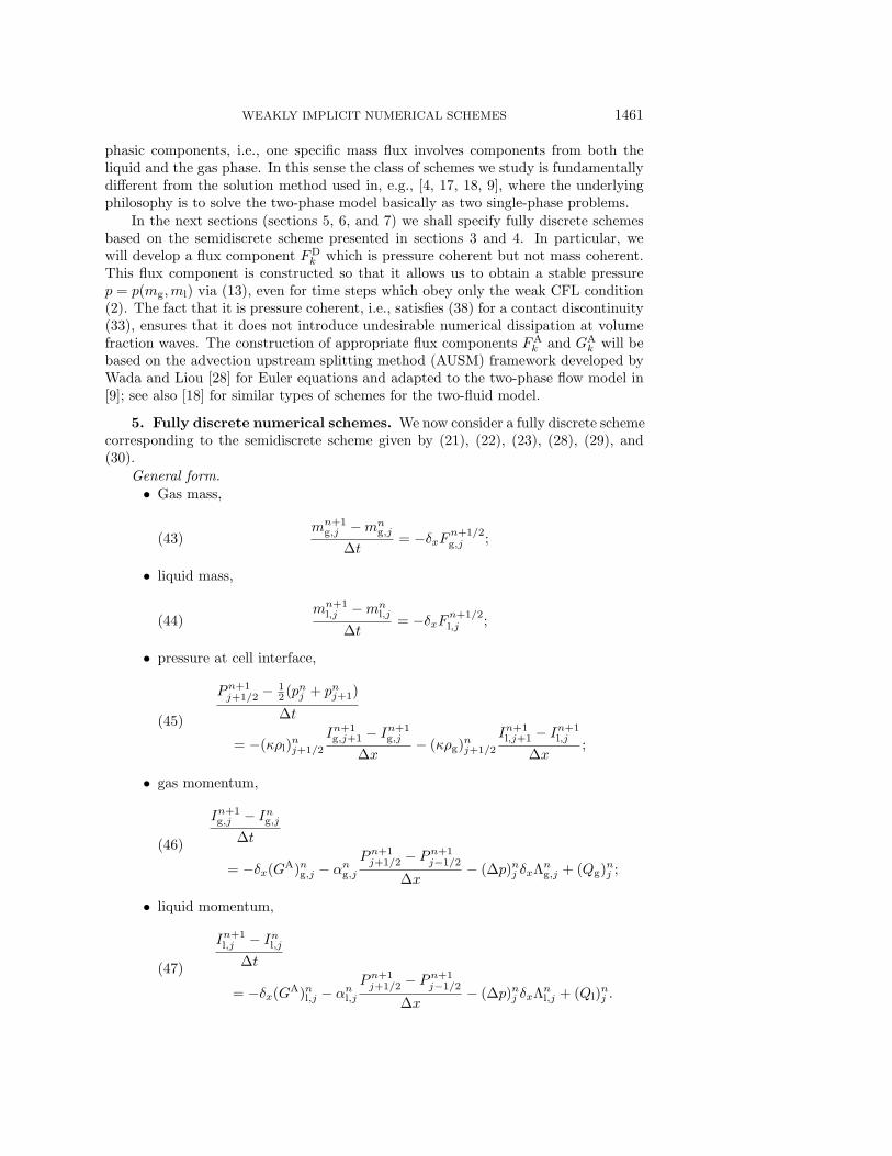
Fig. 5. Water faucet problem, 120 cells, T = 0.6 s. Roe versus WIMF-AUSMD, Δx/Δt = 103

m/s. Top left: gas fraction. Top right: pressure. Bottom left: liquid velocity. Bottom right: gasvelocity.

αl(x, t) =

{α0(1 + 2gxv−2

0 )−1/2 for x < v0t + 12gt

2,α0 otherwise,

(76)

where the parameters α0 = 0.8 and v0 = 10 m/s are the initial states.

8.2.1. Comparison with explicit Roe scheme. We now compare the WIMF-AUSMD scheme with the explicit Roe scheme under equal conditions. That is, weassume a grid of 120 cells and use the time step

Δx

Δt= 103 m/s.(77)

Results are given in Figure 5 after t = 0.6 s. We note that there is little visibledifference between WIMF-AUSMD and the Roe scheme on the volume fraction wave.However, the WIMF-AUSMD is somewhat more diffusive on pressure. This is consis-tent with our observations in section 8.1.1.

8.2.2. Effect of increasing the time step for WIMF-AUSMD. An eigen-value analysis (see [26, 9]) reveals that the velocities of the volume fraction waves areapproximately given by

λ±v =

ρgαlvg + ρlαgvl

ρgαl + ρlαg±√

Δp(ρgαl + ρlαg) − ρlρgαlαg(vg − vl)2

(ρgαl + ρlαg)2.(78)


0.2

0.25

0.3

0.35

0.4

0.45

0.5

0.55

0 2 4 6 8 10 12

Gas

frac

tion

Distance (m)

reference14 m/s17 m/s25 m/s

1000 m/s

99600

99650

99700

99750

99800

99850

99900

99950

100000

0 2 4 6 8 10 12

Pre

ssur

e (P

a)

Distance (m)

Roe 1200 cells14 m/s17 m/s25 m/s

1000 m/s

10

11

12

13

14

15

16

17

0 2 4 6 8 10 12

Liqu

id v

eloc

ity (

m/s

)

Distance (m)

reference14 m/s17 m/s25 m/s

1000 m/s

-25

-20

-15

-10

-5

0

5

0 2 4 6 8 10 12

Gas

vel

ocity

(m

/s)

Distance (m)

14 m/s17 m/s25 m/s

1000 m/s

Fig. 6. Water faucet problem, 120 cells, T = 0.6 s. Different time steps for the WIMF-AUSMDscheme. Top left: gas fraction. Top right: pressure. Bottom left: liquid velocity. Bottom right: gasvelocity.

For a weakly implicit scheme as defined by (2) we must then have

Δx

Δt≥ max

j,n(λ±

v ).(79)

Having ρl >> ρg we obtain from (78)

λ±v ≈ vl,(80)

and hence we expect a weakly implicit scheme to encounter CFL-related stabilityproblems near time steps corresponding to the liquid velocity.

We now study the effect of increasing the time step for the WIMF-AUSMD scheme.We consider the following time steps:

• Δx/Δt = 1000 m/s,• Δx/Δt = 25 m/s,• Δx/Δt = 17 m/s,• Δx/Δt = 14 m/s.

Results for these time steps are given in Figure 6. We observe that increasing the timestep toward the time step corresponding to the liquid velocity significantly improvesthe accuracy of WIMF-AUSMD on the volume fraction wave, as seen on the plots ofvelocities and volume fraction. The rate of improvement in accuracy is largest nearthe optimal time step Δx/Δt = vl. Increasing the time step further violates the weakCFL criterion (79) and instabilities occur. The increased accuracy in volume fractionis accompanied by increased numerical dissipation in the pressure variable, consistentwith our observations in section 8.1.2.


0.2

0.25

0.3

0.35

0.4

0.45

0.5

0 2 4 6 8 10 12

Gas

frac

tion

Distance (m)

referenceWIMF-AUMSD

Roe

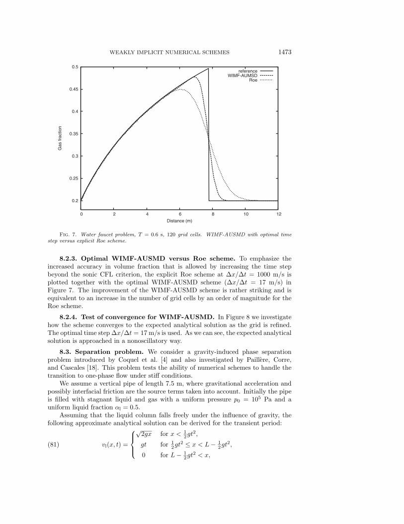
Fig. 7. Water faucet problem, T = 0.6 s, 120 grid cells. WIMF-AUSMD with optimal timestep versus explicit Roe scheme.

8.2.3. Optimal WIMF-AUSMD versus Roe scheme. To emphasize theincreased accuracy in volume fraction that is allowed by increasing the time stepbeyond the sonic CFL criterion, the explicit Roe scheme at Δx/Δt = 1000 m/s isplotted together with the optimal WIMF-AUSMD scheme (Δx/Δt = 17 m/s) inFigure 7. The improvement of the WIMF-AUSMD scheme is rather striking and isequivalent to an increase in the number of grid cells by an order of magnitude for theRoe scheme.

8.2.4. Test of convergence for WIMF-AUSMD. In Figure 8 we investigatehow the scheme converges to the expected analytical solution as the grid is refined.The optimal time step Δx/Δt = 17 m/s is used. As we can see, the expected analyticalsolution is approached in a nonoscillatory way.

8.3. Separation problem. We consider a gravity-induced phase separationproblem introduced by Coquel et al. [4] and also investigated by Paillere, Corre,and Cascales [18]. This problem tests the ability of numerical schemes to handle thetransition to one-phase flow under stiff conditions.

We assume a vertical pipe of length 7.5 m, where gravitational acceleration andpossibly interfacial friction are the source terms taken into account. Initially the pipeis filled with stagnant liquid and gas with a uniform pressure p0 = 105 Pa and auniform liquid fraction αl = 0.5.

Assuming that the liquid column falls freely under the influence of gravity, thefollowing approximate analytical solution can be derived for the transient period:

vl(x, t) =

⎧⎪⎨⎪⎩√

2gx for x < 12gt

2,

gt for 12gt

2 ≤ x < L− 12gt

2,

0 for L− 12gt

2 < x,

(81)


0.2

0.25

0.3

0.35

0.4

0.45

0.5

0 2 4 6 8 10 12

Gas

frac

tion

Distance (m)

reference1200 cells120 cells60 cells24 cells12 cells6 cells

Fig. 8. Water faucet problem, T = 0.6 s. Grid refinement for the WIMF-AUSMD scheme.

αl(x, t) =

⎧⎪⎨⎪⎩

0 for x < 12gt

2,

0.5 for 12gt

2 ≤ x < L− 12gt

2,

1 for L− 12gt

2 < x,

(82)

where L = 7.5 m is the length of the tube. This approximate solution consists of acontact discontinuity at the top of the tube and a shock-like discontinuity at the lowerpart of the tube. After the time

T =

√L

g= 0.87 s(83)

these discontinuities will merge and the phases will become fully separated. Thevolume fraction reaches a stationary state, whereas the other variables slowly con-verge toward a stationary solution. Assuming hydrostatic conditions the pressure willapproximately be given by

p(x, t) =

{p0 for x < L/2,

p0 + ρlg (x− L/2) for x ≥ L/2.(84)

8.3.1. Transition to one-phase flow. We observed that the basic WIMF-AUSMD scheme would produce instabilities in the transition to one-phase flow. In-deed, this is a common problem for two-phase flow models, observed by, among others,Coquel et al. [4] for their kinetic scheme, Paillere, Corre, and Cascales [18] for theirAUSM+ scheme, and Romate [21] for his Roe scheme. Romate suggested a schemeswitching strategy for solving this problem, where the original scheme is replacedwith a stable, diffusive scheme near one-phase regions. Here we will follow a similarapproach, using a strategy that has been previously applied with success [9]. Weproceed as follows.


8.3.2. Modification of basic AUSMV and AUSMD splitting formulas.We modify the parameters χ used in the splitting formulas (60) corresponding to theAUSMV and AUSMD schemes,

χL = (1 − φL)2(ρ/α)L

(ρ/α)L + (ρ/α)R+ φL(85)

and

χR = (1 − φR)2(ρ/α)R

(ρ/α)L + (ρ/α)R+ φR,(86)

for each phase. Here φ is the transition fix function

φ = φ(αg) = e−Γgαg + e−Γl(1−αg),(87)

where Γk is a parameter controlling the diffusive effect of the transition fix. This fixensures that we recover the more stable FVS/van Leer fluxes, as given by (56)–(59),in one-phase regions.

We observe that the transition to one-phase liquid flow (the denser phase) moreeasily induces instabilities than the transition to one-phase gas flow (the less densephase). For the purposes of this paper, we choose the parameters

Γg = 50(88)

and

Γl = 500.(89)

Definition 8. The modified AUSMD scheme as described by (85) and (86)will be denoted as the AUSMD∗ scheme. Similarly, the modified AUSMV scheme asdescribed by (85) and (86) will be denoted as the AUSMV∗ scheme.

8.3.3. WIMF-AUSMDV∗. We consider convective fluxes which are a hybridof those employed by AUSMD∗ and AUSMV∗ and are denoted as AUSMDV∗. Moreprecisely, the numerical convective fluxes (αρv)j+1/2 and (αρv2)j+1/2 are given by thefollowing expression:

(αρv)AUSMDV∗

j+1/2 = s(αρv)AUSMV∗

j+1/2 + (1 − s)(αρv)AUSMD∗

j+1/2 ,

(αρv2)AUSMDV∗

j+1/2 = s(αρv2)AUSMV∗

j+1/2 + (1 − s)(αρv2)AUSMD∗

j+1/2 .(90)

Here s is chosen as

s = max(φL, φR),(91)

where φ is the transition fix function given by (87). Note that this hybridizationaffects only the momentum convective fluxes since (αρv)AUSMV∗

j+1/2 = (αρv)AUSMD∗

j+1/2 .

The construction (90) ensures that AUSMDV∗ uses the accurate AUSMD∗ fluxesin two-phase regions and switches to the more stable AUSMV∗ fluxes in one-phaseregions.

The WIMF-AUSMDV∗ scheme is now constructed straightforwardly by associat-ing the fluxes FA

k and GAk with the corresponding AUSMDV∗ fluxes as follows.


Definition 9. We will use the term WIMF-AUSMDV∗ to denote the numer-ical scheme given by (43)–(50), where (FD

k )n+1/2j+1/2 is given by the pressure coherent

component (55) whereas (FAk )nj+1/2 and (GA


(FAk )nj+1/2 = (ραv)AUSMDV∗,n

k,j+1/2 , (GAk )nj+1/2 = (ραv2)AUSMDV∗,n

k,j+1/2 .

Remark 11. It should be noted that we have no formal proof which guaran-tees that negative mass fractions will never be calculated by the proposed WIMF-AUSMDV∗ scheme. It does, however, work well on practical cases, while retainingthe property of being fully consistent with the model formulation.

The idea of increasing the numerical dissipation near one-phase regions may beexplored more systematically with the aim of obtaining more general relations thatdo not involve free parameters. Paillere, Corre, and Cascales [18] used a relatedapproach, introducing a diffusion term depending on the pressure gradient to improvethe performance of their AUSM+ scheme near one-phase liquid regions.

8.3.4. Numerical results. We now consider two different formulations of thetwo-fluid model:

• Frictionless flow. We assume that gravity is the only source term taken intoaccount. In this case, the lack of friction terms causes the gas velocity tobecome large as the gas phase is disappearing. We note that for one-phaseliquid flow we have αl >> αg and the volume fraction velocities (78) aredominated by this large gas velocity. Hence the weak CFL criterion (79)becomes very restrictive here. With this model we use the relatively low timestep

Δx

Δt= 500 m/s.(92)

For stability of the FVS scheme, which AUSMDV∗ employs in the transi-tion to single phase flow, we rescale the sound velocity c as described in theappendix, using

c = 750 m/s(93)

instead of the sound velocity determined from (12). This choice was basedon the fact that we observed that the gas velocity could become as high asapproximately 400 m/s. According to (120) in the appendix, we should thenchoose c such that 200 ≤ c ≤ 800. We consistently have chosen c in the upperregion.

• Interfacial momentum exchange. The low time step needed for the friction-less model is undesirable. In addition, the assumption of frictionless low isunphysical. In reality we expect the last remnants of the disappearing phaseto be completely dissolved, and we expect vg ≈ vl near one-phase regions. Tomore realistically model this situation, we consider an interfacial momentumtransfer model also used by Paillere, Corre, and Cascales [18]. For the gasmomentum equation, we introduce the source term

MDg = Cαgαlρg(vg − vl),(94)

where C is a positive constant. Likewise, the liquid momentum source termis given as

MDl = −MD

g = −Cαgαlρg(vg − vl),(95)


conserving total momentum. We write

C = C0φ,(96)

making the exchange term kick in more strongly near one-phase regions. Fol-lowing [18], we set

C0 = 50000 s−1.(97)

To avoid stability problems related to stiffness in this term, we use a semi-implicit implementation as follows:

(MDg )

n+1/2j = Cn

j (αgαlρg)nj

[(Ig)

n+1j

(mg)nj−

(Il)n+1j

(ml)nj

].(98)

We found that we could now increase the time step to

Δx

Δt= 75 m/s,(99)

consistent with the largest gas (volume fraction) velocities during the tran-sient period. The sound velocity is rescaled as

c = 150 m/s.(100)

Again, this choice is based on the criterion (120), where we now can assumethat the fluid velocity becomes zero in the transition to single-phase flow (dueto the inclusion of the interfacial momentum transfer model). This gives usthat c should be chosen in the interval 0 ≤ c ≤ 2λ = 2Δx/Δt.

Results after t = 0.6 s are plotted in Figure 9, using a grid of 100 cells. Theapproximate analytical solutions (81) and (82) are used for reference. We note thatgood accordance with the expected analytical solutions is achieved. The most notableeffect of the interfacial momentum exchange term is the reduction of the gas velocityin the one-phase liquid region.

Although the phases will be separated for t < 1.0 s, it takes some seconds beforethe excess momentum has been dissipated at the endpoints. Results for fully station-ary conditions (t = 5.0 s) are plotted in Figure 10. We note that the frictionless modeldoes not exactly yield the expected hydrostatic pressure distribution. This seems tobe due to the strong velocity gradients at the separation point, and hydrostatic con-ditions are never fully reached. The inclusion of the interfacial friction term removesthese gradients.

In Figure 11 the effect of grid refinement on the resolution of volume fraction isillustrated for the WIMF-AUSMDV∗ scheme with momentum exchange terms. Thetime step Δx/Δt = 75 m/s is used. The expected analytical solution is approachedin a monotone way.

8.4. Oscillating manometer problem. Finally, we consider a problem intro-duced by Ransom [20] and investigated by Paillere, Corre, and Cascales [18] and Evjeand Flatten [9]. This problem tests the ability of numerical schemes to handle achange in the flow direction.


0

0.2

0.4

0.6

0.8

1

0 1 2 3 4 5 6 7

Liqu

id fr

actio

n

Distance (m)

referenceno friction

friction

90000

100000

110000

120000

130000

140000

150000

160000

0 1 2 3 4 5 6 7

Pre

ssur

e (P

a)

Distance (m)

no frictionfriction

0

1

2

3

4

5

6

0 1 2 3 4 5 6 7

Liqu

id v

eloc

ity (

m/s

)

Distance (m)


friction

-180

-160

-140

-120

-100

-80

-60

-40

-20

0

0 1 2 3 4 5 6 7

Gas

vel

ocity

(m

/s)

Distance (m)

no frictionfriction

Fig. 9. Separation problem, T = 0.6 s, 100 grid cells. WIMF-AUSMDV∗ scheme with andwithout interfacial momentum exchange terms. Top left: liquid fraction. Top right: pressure.Bottom left: liquid velocity. Bottom right: gas velocity.

We consider a U-shaped tube of total length 20 m. The geometry of the tube isreflected in the x-component of the gravity field

gx(x) =

⎧⎪⎪⎨⎪⎪⎩

g for 0 ≤ x ≤ 5 m,

g cos(

(x−5 m)10 m π

)for 5 m < x ≤ 15 m,

−g for 15 m < x ≤ 20 m.

(101)

Initially we assume that the liquid fraction is given by

αl(x) =

⎧⎪⎨⎪⎩

10−6 for 0 ≤ x ≤ 5 m,

0.999 for 5 m < x ≤ 15 m,

10−6 for 15 m < x ≤ 20 m.

(102)

The initial pressure is assumed to be equal to the hydrostatic pressure distribution. Weassume that the gas velocity is uniformly vg = 0, and the liquid velocity distributionis given by

vl(x) =

⎧⎪⎨⎪⎩

0 for 0 ≤ x ≤ 5 m,

V0 for 5 m < x ≤ 15 m,

0 for 15 m < x ≤ 20 m,

(103)

where V0 = 2.1 m/s.


0

0.2

0.4

0.6

0.8

1

0 1 2 3 4 5 6 7

Liqu

id fr

actio

n

Distance (m)


friction

95000

100000

105000

110000

115000

120000

125000

130000

135000

140000

0 1 2 3 4 5 6 7

Liqu

id fr

actio

n

Distance (m)


friction

-0.5

0

0.5

1

1.5

2

2.5

3

3.5

4

4.5

5

0 1 2 3 4 5 6 7

Liqu

id v

eloc

ity (

m/s

)

Distance (m)

no frictionfriction

-250

-200

-150

-100

-50

0

50

0 1 2 3 4 5 6 7

Gas

vel

ocity

(m

/s)

Distance (m)

no frictionfriction

Fig. 10. Separation problem, t = 5.0 s, 100 grid cells. WIMF-AUSMDV∗ scheme with andwithout interfacial momentum exchange terms. Top left: liquid fraction. Top right: pressure.Bottom left: liquid velocity. Bottom right: gas velocity.

0

0.2

0.4

0.6

0.8

1

0 1 2 3 4 5 6 7

Liqu

id fr

actio

n

Distance (m)

reference1000 cells100 cells25 cells

Fig. 11. Separation problem, T = 0.6 s. Convergence properties of the WIMF-AUSMDV∗

scheme with interfacial momentum exchange terms.


-2

-1

0

1

2

3

0 5 10 15 20

Liqu

id v

eloc

ity (

m/s

)

Time (s)

reference500 cells100 cells

Fig. 12. Oscillating manometer, WIMF-AUSMDV∗ scheme. Time development of the liquidvelocity.

Ransom [20] suggested treating the manometer as a closed loop. We will followthe approach of Paillere, Corre, and Cascales [18], assuming that both ends of themanometer are open to the atmosphere. We assume that the liquid column will movewith uniform velocity under the influence of gravity, giving the following approximateanalytical solution for the liquid velocity [18]

vl(t) = V0 cos(ωt),(104)

where

ω =

√2g

L,(105)

where L = 10 m is the length of the liquid column.To exploit the possibility of taking large time steps, we include the interfacial

momentum exchange term as described in section 8.3.4. The sound velocity is rescaledto c = 30 m/s, which is consistent with (120), where we use that the fluid velocity isnegligible in the transition to single-phase flow.

8.4.1. Numerical results. We consider the following grids:• 100 cells—we use a time step corresponding to Δx/Δt = 50 m/s, and• 500 cells—we use a time step corresponding to Δx/Δt = 15 m/s.

For the fine grid with 500 cells, the critical time step was found to be consistent withthe weak CFL criterion (79). For the coarse grid consisting of 100 cells, a lower CFLnumber was needed to ensure stability. The evolution of the center cell liquid velocityis given in Figure 12. We note that the results for 100 and 500 cells are virtuallyidentical, indicating that the resolution of the liquid velocity is not grid sensitive. We


0

0.1

0.2

0.3

0.4

0.5

0.6

0.7

0.8

0.9

1

0 2 4 6 8 10 12 14 16 18 20

Liqu

id fr

actio

n

Distance (m)

WIMF-AUSMDV*

100000

105000

110000

115000

120000

125000

130000

135000

0 2 4 6 8 10 12 14 16 18 20

Pre

ssur

e (P

a)

Distance (m)

WIMF-AUSMDV*

-4

-3.5

-3

-2.5

-2

-1.5

-1

-0.5

0

0 2 4 6 8 10 12 14 16 18 20

Liqu

id v

eloc

ity (

m/s

)

Distance (m)

WIMF-AUSMDV*

-4.5

-4

-3.5

-3

-2.5

-2

-1.5

-1

-0.5

0

0.5

0 2 4 6 8 10 12 14 16 18 20

Gas

vel

ocity

(m

/s)

Distance (m)

WIMF-AUSMDV*

Fig. 13. Oscillating manometer, t = 20.0 s, 500 grid cells. WIMF-AUSMDV∗ scheme. Topleft: liquid fraction. Top right: pressure. Bottom left: liquid velocity. Bottom right: gas velocity

observe a slight phase difference from the approximate analytical solution, as was alsoobserved in [18, 9].

The distribution of all variables after t = 20 s is given in Figure 13 for the gridof 500 cells. We observe that the variables are approximated without any numericaloscillations. In particular there is little numerical diffusion for the volume fractionvariable. The strong gradients in the velocities are a consequence of the sudden volumechange at the transition points between the phases. We remark that the gas velocitywas extrapolated at the boundaries, whereas the liquid velocity was forced to zero atthe boundaries to avoid liquid mass leakage.

9. Summary. We have proposed a general framework for constructing weaklyimplicit methods for a two-fluid model. Particularly, we have constructed a weaklyimplicit numerical scheme, denoted as WIMF-AUSMD, that allows the CFL criterionfor sonic waves to be violated. All the numerical experiments indicate that a weakerCFL criterion applies with relation to the slow-moving volume fraction waves.

The scheme is based on a mixture flux approach which properly combines diffusiveand nondissipative fluxes to yield an accurate and robust resolution of sonic andvolume fraction waves on nonstaggered grids. The sonic CFL criterion is violated byenforcing a coupling between the pressure wave component of the mixture flux, thecell center momenta, and the cell interface pressure. In particular all convective (massand momentum) fluxes are treated in an explicit manner.

The numerical evidence indicates that the WIMF-AUSMD is highly robust andefficient and gives an accuracy potentially superior to the explicit Roe scheme onvolume fraction waves. An added advantage of the WIMF-AUSMD scheme is that


it does not require a full eigenstructure decomposition of the Jacobi matrix for thesystem. However, the scheme is diffusive on pressure waves, especially for large timesteps.

By increasing the numerical dissipation near one-phase regions, we have demon-strated that the framework allows for accurate, efficient, and robust solutions also forflow cases which locally involve the transition from one-phase to two-phase flow.

Appendix.

Rescaling the sound velocity. A problem with the original FVS scheme isthat it can produce instabilities for large time steps if the discretization parameterλ = Δx/Δt is chosen much smaller than the sound velocity. For an explicit schemethis will never be a problem as the CFL criterion limits the time steps we can take.For a semi-implicit method, however, we wish to use a value for λ that may be severalorders of magnitude smaller than the physical sound velocity and the issue becomesof relevance. To describe the problem, we consider the mass conservation equation

∂u

∂t+

∂(uv)

∂x= 0,(106)

where u = ρkαk. We now consider the FVS scheme

(uv)j+1/2 = V +(vj , c)uj + V −(vj+1, c)uj+1,(107)

where we use the splitting formulas (56), assuming v < c,

V ±(v, c) = ± 1

4c(v ± c)2.(108)

Total variation stability. We now take advantage of the following theorem dueto Harten, as stated by Tadmor [24]

Theorem 1. Consider the scalar equation

∂u

∂t+

∂f(u)

∂x= 0(109)

solved by the numerical scheme

un+1j − uj

Δt+

1

Δx

(F(un

j , unj+1) − F(un

j−1, unj ))

= 0,(110)

where the numerical flux F(unj , u

nj+1) is written in viscous form

Fj+1/2 = F(unj , u

nj+1) =

1

2

(f(un

j ) + f(unj+1)

)− 1

2

Δx

ΔtQn

j+1/2(unj+1 − un

j ).(111)

The scheme (110) is total variation nonincreasing provided its numerical viscositycoefficient Qn

j+1/2 = Q(unj , u

nj+1) satisfies

Δt

Δx

∣∣∣∣∣f(unj+1) − f(un

j )

unj+1 − un

j

∣∣∣∣∣ ≤ Qnj+1/2 ≤ 1.(112)

For the scheme (107) using the splitting formulas (108) we obtain the numericalviscosity coefficient

Qnj+1/2 =

Δt

Δx

v2 + c2

2c.(113)


Using this and assuming uniform velocity we can write the requirement (112) as

Δt

Δxv ≤ Δt

Δx

v2 + c2

2c≤ 1,(114)

which yields the following lemma.Lemma 3. Let the mass equation (106) be solved using the numerical fluxes given

by (107) and (108). Then the resulting scheme is total variation nonincreasing if

Δx

Δt≥ v2 + c2

2c(115)

and

c > 0.(116)

The criterion (115) attains its minimum value for v = c, for which we obtain

Δx

Δt≥ v,(117)

which is the standard CFL criterion.To further investigate how c should be chosen, we now assume that

λ =Δx

Δt(118)

is known and investigate which criteria govern the possible choices for c. From (115)we obtain

c2 − 2cλ + v2 ≤ 0.(119)

Solving this equation we obtain the following corollary.Corollary 1. Let the linear advection equation (106) be solved using the numer-

ical fluxes given by (107) and (108). Assume the time step λ = Δx/Δt is known. Thenthe resulting scheme is total variation nonincreasing if the sound velocity c satisfies

λ−√λ2 − v2 ≤ c ≤ λ +

√λ2 − v2.(120)

This result is confirmed by numerical experiments and illustrates that if c >> λthe FVS scheme is unstable. We hence propose to rescale the sound velocity used inthe flux splitting schemes such that the requirement (120) is satisfied also for largetime steps. We stress that this step is necessary to achieve stability on the advectiveeffects for the FVS scheme. Stability of the sonic waves is an independent problemthat we wish to achieve through taking advantage of the implicit pressure-momentumcoupling together with the decomposition of Fk into FD

k and FAk .

Acknowledgments. The authors thank the reviewers for carefully readingthrough the manuscript and making several useful comments.


REFERENCES

[1] R. Abgrall, How to prevent pressure oscillations in multicomponent flow calculations, J. Com-put. Phys., 125 (1996), pp. 150–160.

[2] F. Barre and M. Bernard, The cathare code strategy and assessment, Nuclear Engrg. Des.,124 (1990), pp. 257–284.

[3] K. H. Bendiksen, D. Malnes, R. Moe, and S. Nuland, The dynamic two-fluid model OLGA:Theory and application, SPE Prod. Eng., 6 (1991), pp. 171–180.

[4] F. Coquel, K. El Amine, E. Godlewski, B. Perthame, and P. Rascle, A numerical methodusing upwind schemes for the resolution of two-phase flows, J. Comput. Phys., 136 (1997),pp. 272–288.

[5] J. Cortes, A. Debussche, and I. Toumi, A density perturbation method to study the eigen-structure of two-phase flow equation systems, J. Comput. Phys., 147 (1998), pp. 463–484.

[6] J. R. Edwards, R. K. Franklin, and M.-S. Liou, Low-diffusion flux-splitting methods forreal fluid flows with phase transition, AIAA J., 38 (2000), pp. 1624–1633.

[7] S. Evje and K. K. Fjelde, Hybrid flux-splitting schemes for a two-phase flow model, J. Com-put. Phys., 175 (2002), pp. 674–701.

[8] S. Evje and K. K. Fjelde, On a rough AUSM scheme for a one-dimensional two-phase flowmodel, Comput. & Fluids, 32 (2003), pp. 1497–1530.

[9] S. Evje and T. Flatten, Hybrid flux-splitting schemes for a common two-fluid model, J. Com-put. Phys., 192 (2003), pp. 175–210.

[10] I. Faille and E. Heintze, A rough finite volume scheme for modeling two-phase flow in apipeline, Comput. & Fluids, 28 (1999), pp. 213–241.

[11] K.-K. Fjelde and K. H. Karlsen, High-resolution hybrid primitive-conservative upwindschemes for the drift flux model, Comput. & Fluids, 31 (2002), pp. 335–367.

[12] M. Larsen, E. Hustvedt, P. Hedne, and T. Straume, Petra: A novel computer code forsimulation of slug flow, in SPE Annual Technical Conference and Exhibition, Society ofPetroleum Engineers, 1997.

[13] M.-S. Liou, A sequel to AUSM: AUSM(+), J. Comput. Phys., 129 (1996), pp. 364–382.[14] J. M. Masella, Q. H. Tran, D. Ferre, and C. Pauchon, Transient simulation of two-phase

flow in pipes, Int. J. Multiphase Flow, 24 (1998), pp. 739–755.[15] J. M. Masella, I. Faille, and T. Gallouet, On an approximate Godunov scheme, Int. J.

Comput. Fluid. Dyn., 12 (1999), pp. 133–149.[16] Y. Y. Niu, Simple conservative flux splitting for multi-component flow calculations, Num. Heat

Trans., 38 (2000), pp. 203–222.[17] Y.-Y. Niu, Advection upwinding splitting method to solve a compressible two-fluid model, In-

ternat. J. Numer. Methods Fluids, 36 (2001), pp. 351–371.[18] H. Paillere, C. Corre, and J. R. G Cascales, On the extension of the AUSM+ scheme to

compressible two-fluid models, Comput. & Fluids, 32 (2003), pp. 891–916.[19] S. V. Patankar, Numerical Heat Transfer and Fluid Flow, Taylor & Francis, Philadelphia,

1980.[20] V. H. Ransom, Numerical benchmark tests, Multiphase Sci. Tech., 3 (1987), pp. 465–473.[21] J. E. Romate, An approximate Riemann solver for a two-phase flow model with numerically

given slip relation, Comput. & Fluids, 27 (1998), pp. 455–477.[22] R. Saurel and R. Abgrall, A multiphase Godunov method for compressible multifluid and

multiphase flows, J. Comput. Phys., 150 (1999), pp. 425–467.[23] R. Saurel and R. Abgrall, A simple method for compressible multifluid flows, SIAM J. Sci.

Comput., 21 (1999), pp. 1115–1145.[24] E. Tadmor, Numerical viscosity and the entropy condition for conservative difference schemes,

Math. Comp., 43 (1984), pp. 369–381.[25] I. Toumi, An upwind numerical method for two-fluid two-phase flow models, Nuclear Sci.

Engrg., 123 (1996), pp. 147–168.[26] I. Toumi and A. Kumbaro, An approximate linearized riemann solver for a two-fluid model,

J. Comput. Phys., 124 (1996), pp. 286–300.[27] J. A. Trapp and R. A. Riemke, A nearly-implicit hydrodynamic numerical scheme for two-

phase flows, J. Comput. Phys., 66 (1986), pp. 62–82.[28] Y. Wada and M.-S. Liou, An accurate and robust flux splitting scheme for shock and contact

discontinuities, SIAM J. Sci. Comput., 18 (1997), pp. 633–657.

Documents

WEAKLY IMPLICIT NUMERICAL SCHEMES - UiSsevje/files/1-60063.pdfThe aim of this paper is to construct semi-implicit numerical schemes for a two-phase (two-ﬂuid) ﬂow model, allowing