Embed Size (px)
Citation preview

econstorMake Your Publication Visible
A Service of
zbwLeibniz-InformationszentrumWirtschaftLeibniz Information Centrefor Economics
Hartog, Joop; Gerritsen, Sander
Working Paper
Mincer Earnings Functions for the Netherlands1962-2012
CESifo Working Paper, No. 5719
Provided in Cooperation with:Ifo Institute – Leibniz Institute for Economic Research at the University ofMunich
Suggested Citation: Hartog, Joop; Gerritsen, Sander (2016) : Mincer Earnings Functions for theNetherlands 1962-2012, CESifo Working Paper, No. 5719
This Version is available at:http://hdl.handle.net/10419/128419
Standard-Nutzungsbedingungen:
Die Dokumente auf EconStor dürfen zu eigenen wissenschaftlichenZwecken und zum Privatgebrauch gespeichert und kopiert werden.
Sie dürfen die Dokumente nicht für öffentliche oder kommerzielleZwecke vervielfältigen, öffentlich ausstellen, öffentlich zugänglichmachen, vertreiben oder anderweitig nutzen.
Sofern die Verfasser die Dokumente unter Open-Content-Lizenzen(insbesondere CC-Lizenzen) zur Verfügung gestellt haben sollten,gelten abweichend von diesen Nutzungsbedingungen die in der dortgenannten Lizenz gewährten Nutzungsrechte.
Terms of use:
Documents in EconStor may be saved and copied for yourpersonal and scholarly purposes.
You are not to copy documents for public or commercialpurposes, to exhibit the documents publicly, to make thempublicly available on the internet, or to distribute or otherwiseuse the documents in public.
If the documents have been made available under an OpenContent Licence (especially Creative Commons Licences), youmay exercise further usage rights as specified in the indicatedlicence.
www.econstor.eu

Mincer Earnings Functions for the Netherlands 1962-2012
Joop Hartog Sander Gerritsen
CESIFO WORKING PAPER NO. 5719 CATEGORY 5: ECONOMICS OF EDUCATION
JANUARY 2016
An electronic version of the paper may be downloaded • from the SSRN website: www.SSRN.com • from the RePEc website: www.RePEc.org
• from the CESifo website: Twww.CESifo-group.org/wp T
ISSN 2364-1428

CESifo Working Paper No. 5719
Mincer Earnings Functions for the Netherlands 1962-2012
Abstract We extract estimation results on the Mincer earnings function from four earlier studies and add new results from a recent dataset. We analyse differences related to differences in earnings concepts, in sampling frame and differences among studies that cannot be explained. Jointly, the studies show a clear U-shaped development in the rate of return to education from 1962 to 2012, with a bottom in the 1980’s. We explain this from Tinbergens’s race between suppy and demand (schooling and technology) and suggest this may be a widespread international pattern. Returns to potential experience show no marked time trend.
JEL-codes: I260, J240, J310.
Keywords: returns to education, Mincer earnings equation, race supply and demand.
Joop Hartog* University of Amsterdam
P.O. Box 15867 The Netherlands – 1001 NJ Amsterdam
Sander Gerritsen CPB Netherlands Bureau
for Economic Policy Analysis The Netherlands - 2585 JR The Hague
*corresponding author The paper has been presented at the CPB-OCW Workshop “Returns to education: research and policy”, The Hague, December 17 2015. We are grateful to Bas ter Weel and Harry Patrinos for comments on an earlier version and to Wiljan van den Berge and Dinand Webbink for providing us with their data.

[1] Concept Notulen LOWI-bijeenkomst 9 december 2014
2
1. The Mincer equation
The Mincer earnings equation is a standard summary of the wage structure by education and
experience:
2
0 1 2 3lnW S X X
Ln W is the logarithm of an employee’s wage rate per time unit, S is years of schooling, X is years of
work experience and is a residual for all other variables; some of these other variables may be
explicitly specified (e.g. gender or region). The equation has at well defined theoretical basis in the
theory of human capital. Under strict conditions, 1 can be interpreted as the rate of return on
investment in schooling: the return on invested foregone wages by going to school rather than going to
work. Key conditions are perfect competition in the labour market, stationarity across cohorts,
identical aptness among individuals to benefit from schooling (equal “ability”), negligible tuition and
other direct cost of schooling, linearity of returns in years of schooling and separabity of log earnings
in schooling and experience. 2 and 3 measure the returns to continued investment after school, in
on-the-job training. Because of easier data availability, X is commonly measured as potential
experience: age minus age of graduation from highest level of schooling attended. In standard
applications, years of schooling S is measured as the normal, nominal duration of an education. OLS
estimates cannot be taken as measures of causal effects, essentially because benefits can only be
inferred from individuals who differ in the amount of schooling they have chosen1. Without the frame
of human capital theory, the equation measures the effect of an extra year of schooling and the average
effect of additional experience, from observations on inidividuals that differ in years of schooling and
(potential) experience.
In the next two sections we first present the datasets and then the estimation results from the four
established studies and from our own new study. Section 4 gives an interpretation of the observed U-
shaped time profiles of the Mincer rate of return, section 5 compares the profile to international
evidence, section 6 asks the question to what extent other or further explanations than a race between
supply and demand are needed, and section 7 discusses the proper econometric interpretation of
Mincer returns estimated by OLS. Section 8 concludes.
2. Data
In this paper we present estimation results for The Netherlands from different studies for the period
1962-20122. Unfortunately, not all data have been collected in the same way and we have to face the
issue of comparability. We will present published estimates from 4 studies and results from new
estimations of our own.
HOT3, 1962-1989, CBS loonstructuuronderzoeken combined with NPAO and OSA surveys; gross
1 For discussion and references, see Joop Hartog en Henriette Maassen van den Brink (red), Human capital, theory and
evidence, Cambridge University Press, 2007. For the host of practical issues in data, variable definitions and specifications,
see Harmon, Walker and Westergaard-Nielsen, 2001). 2 We frequently cite verbatim from the source articles, without always specifying the exact location.
3 HOT: J. Hartog, H. Oosterbeek en C. Teulings, Age, wages and education in the Netherlands, in P. Johnson and K.
Zimmermann (eds), Labour markets in an ageing Europe, Cambridge University Press, 1993
[1] Concept Notulen LOWI-bijeenkomst 9 december 2014
3
For the period 1962-1989, data are from 6 samples of 10,000 or more observations, collected from
company administrations by CBS (Central Bureau of Statistics, the national statistical agency). In
1962, 1965 and 1972 observations are sampled from male employees working in manufacturing,
construction and banking, in 1979, 1985 and 1989 from all full-time working men. Up to 1972, there
was a distinction among “employees”, with monthly salary, and “labourers”, with weekly wage,
matching the then internationally common distinction among white-collar and blue-collar workers. The
data are available as mean earnings in cross-tables with 5 levels of education and 6 to 10 age groups. .
In addition, for 1982, 1985, 1986 and 1988 HOT present results based on data collected by NPAO and
OSA (government subsidised programs for labour market research). The data are from national
surveys, each covering some 1200 respondents. Earnings are self-reported, not from administrative
sources.
CBS has published separate cross-table data for labourers in 1972; the survey data for 1982 and 1988
allow to distinguish employees and labourers. Availability of these data permits to assess the effect of
estimating returns on observations for employees only.
SOH4: OSA, 1986-1996; net
Estimates for the period 1986-1996 have been made on data from the bi-annual OSA Labour Market
Panel. The data for each year cover some 4500 individuals aged 16-64. We present results on net
hourly wages, as reported by respondents. Male respondents have a job of 34 hours a week or more,
among females, women with part-time jobs are included and the regressions include a dummy for part-
time work (less than 35 hours a week).
LO5: IALS 1994, NIPO 1999, gross
Leuven and Oosterbeek use two different samples, a survey collected in 1999 by NIPO (an opinion
research agency) and data from the IALS project in 1994 (International Adult Literacy Survey), both
on gross hourly wages for 16-60 year olds. Note that in this case, the data for the two observations of a
“time series” are not from the same sampling frame. The samples are rather small.
JW6: Loonstruktuuronderzoeken 1979-2002; gross
Jacobs and Webbink analyse data from CBS Loonstructuuronderzoeken (Wage Structure Surveys) for
1979, 1985, 1989, 1996, 1997 and 2002: gross hourly wages from administrative sources, calculated
by dividing gross monthly earnings by hours worked.
GH7: CBS Panel Project, 1999-2012;gross
4 SOH: J. Smits, J. Odink en J. Hartog (2000), New results on returns to education in The Netherlands, unpublished note,
University of Amsterdam, Department of Economics and Econometrics; results have been published in J.Hartog, J.Odink
en J.Smits (1999), Rendement op scholing stabiliseert, Economisch-Statistische Berichten, 84 (4215), 13 augustus. 582-
584. 5 LO: E. Leuven en H. Oosterbeek (2000), Rendement van onderwijs stijgt, Economisch-Statistische Berichten,85 (4262).
23 juni, 523-524 6 JW: B. Jacobs en D. Webbink (2006), Rendement onderwijs blijft stijgen, Economisch-Statistische Berichten, 91 (4492),
25 augustus, 406-407; we are grateful to Dinand Webbink for supplying is with his estimation results. 7 GH refers to our own estmates. Earlier estimations on the CBS panel project data were made by D. Webbink, S. Gerritsen
and M. van der Steeg, Financiële opbrengsten onderwijs verder omhoog, ESB 98 (4651). 11 januari 2013. They used annual
rather than hourly wages, leading to rates of return also determined by hours worked. Moreover, years of education was
incorrectly defined: the year of highest education level attained was not not measured in the same year as wages were
observed. Wiljan van den Berge (CPB) kindly provided the data.
[1] Concept Notulen LOWI-bijeenkomst 9 december 2014
4
We present newly estimated returns covering 1999-2012 on data from the CBS Labour Market Panel
Project. We do not use panel observations, but a match of data in the EBB (Enquete Beroepsbevolking,
Labour Force survey) and data in the SSB (Sociaal Statistisch Bestand8, Social Statistical Datasurce).
Earnings are fiscal earnings, taken from the income tax returns and hours worked have been obtained
from EBB. Fiscal earnings are defined as Bruto Loon Sociale Verzekeringen (Gross Earnings Social
Security, BLSV). Earnings have been divided by days worked as applied for Social Security purposes
(SV-dagen) and then divided by daily hours, to arrive at gross hourly wages. Respondents are 16-64
years old, the annual number of observations is between 25 and 30 thousand for men, and between 20
and 25 thousand for women.
3. Results
3.1 Effects of different datasources
Estimates of rates of return on data from different sources, with different definitions and different
sampling frames, cannot be combined at face value in a single time series. Hence, we will first try to
assess effects of these differences. One effect has already been assessed by the original authors
themselves. As noted above, the earliest estimates can be corrected fort he restriction to employees
only. By estimating the Mincer equation on data for employees only and for all workers, from the
same data source in the same year, HOT conclude that estimates on employees only underestimate
returns by 2 percentage points. Experience profiles are not systematically under- or overestimated.
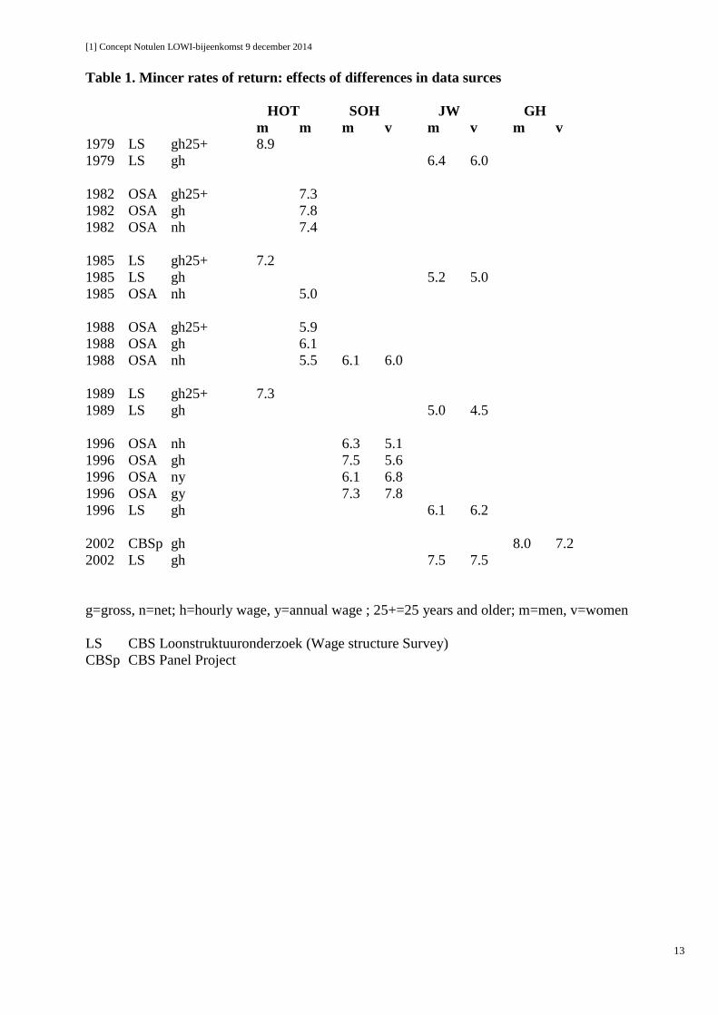
In Table 1 we present estimation results from different data source in the same year. We also estimated
several specifications on the data set used by Webbink, Gerritsen and Van der Steeg (see footnote 7);
we do not present these results, but they have been taken into account in our conclusions.
Age restrictions on the sample have the same effect in all estimations: excluding respondents aged 15-
25 reduces estimated rates of return. The exclusion eliminates in particular early working years of the
low educated, when their earnings increase rapidly. Excluding their low earnings years reduces the gap
with the higher educated, thus depressing the rate of return. The effect of exclusion is larger for
women than for men.
Estimation on net wages generates lower rates of return than estimates on gross wages. This is
plausible from progressive taxation. Yet, caution is warranted as all comparisons between net and
gross are based on self-reported data and not on administrative data. Peculiarities of survey data may
also play a role.
Comparing results from OSA data and CBS Wage Structure Survey data, both for 1996, both on gross
hourly wages, exposes a gap in estimated returns of 1.4 points for men and 0.6 points for women. This
may be due to all kinds of systematic differences in sampling, but it might also simply be due to
random sampling variation. Without further research we have no way to tell them apart.
With our CBS Panel Project data 1999-2012 we have made three estimates, both for men and for
women: no conditions on hours worked, 35 hours a week or more, or all hours but with a dummy for
full-time (35 hours or more). Among men, estimation with a full-time dummy has no effect on the
8 For details on the data, see CBS Centrum voor Beleidsstatistiek, Documentatierapport Arbeidsmarktpanel 1999-2009V1,
30 maart 2012.

[1] Concept Notulen LOWI-bijeenkomst 9 december 2014
5
estimated return to years in school, estimation for full-time workers only increases the schooling
coefficient by 0.005 to 0.006, ie half a percent point. Among women, including a full-time dummy
raises the returns by about one percentage point. Estimation on full-time workers only leads to higher
returns: a difference that gradually increases from 2 to 3 percentage points. Thus, full-time and part-
time workers will not always enjoy identical rates of returns, but intertemporal comparisons are
influenced only slightly for women and not at all for men. Among women, the difference among
estimates without sample constraints on weekly hours and a sample with weekly hours above 34
increases by just more than half a percentage point between 1999 and 2012. We have chosen to present
our results on CBS panel project data from estimation on the sample without restriction on weekly
hours worked.
The Mincer model distinguishes investment in formal schooling and in on-the-job training. To get a
handle on changes in the experience profiles of earnings, we use the estimates to calculate earnings
growth over the first 10 years: 2 310 100 . Results are presented in Table 3.
Restricting the sample to workers over 25 years of age flattens estimated profiles, which comes as no
surprise. The effect is visible in the OSA data 1982 and 1988 as analysed in the HOT study. It is also
visible from the LS data for 1979, 1985 and 1989, but here, the comparison is based on different
studies ( HOT and JW). The profiles are also flatter for net earnings as compared to gross earnings
(OSA 1982, 1988 and 1996), which again, given income tax rate progression, comes as no surprise,
but the effect is mostly modest. Remarkably, profiles for women are mostly flatter for women than for
men before 1999, and mostly steeper after 1999 (in the GH study). This may be a composition effect
on hours worked, as in the GH study women’s profiles are flatter than men’s if only full-time workers
are compared. The profiles estimated by JW are remarkably steeper than in other studies, but this is
due to specification: JW estimate on age rather than potential experience. Smits, Odink and Hartog
(2001, Table 10.7 and Table 10.8)9 estimate on age and on potential experience (age minus schooling
years minus 6) on the same data set (OSA 1996) and find much higher growth rate on age than on
potential experience. For men, the linear terms are 0.081 versus 0.052, for women 0.078 versus 0.041.
3.2 Indications for a time series
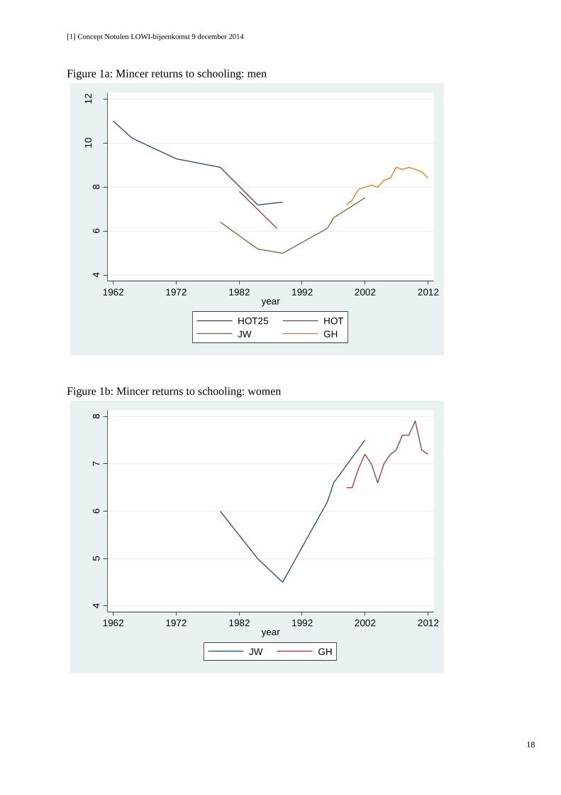
Table 2 and Figure 1 show the development of estimated Mincer returns since 1962. In the graph, we
only connect estimates that emanate from a single study. For men, the composition of fragments
merges into a clear pattern: an asymmetric tulip, starting with a decrease since the early 1960’s
towards a low in the early 1980’s, followed by recovery, after 2007 turnign into a mild decline. The
swings are large. Just considering comparable data points, the initial decrease, from over 12% (when
we add the correction for considering employees only) to some 7% is quite substantial, and the
recovery during the 1990’s, from 5% to 7.5% is also strong. For women, with fewer data points, the
pattern is not at variance with the U-shape observed for men, and the changes are also substantial.
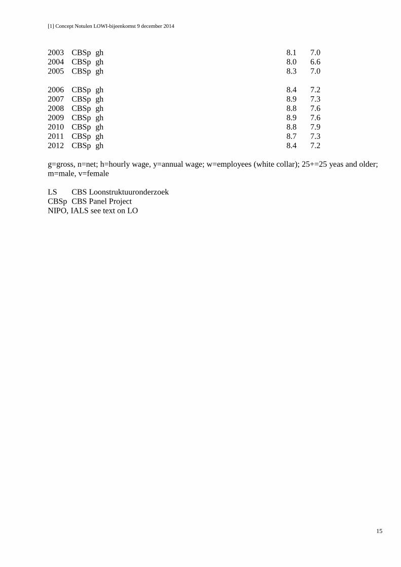
Both for men and for women, the increase from 1999 to the peak in the next decade is some one and a
half percentage point. For both there is a decline during the most recent years.
Just as for the returns to schooling we have graphed (in Figure 2) the ten-year profile slopes,
connecting only the points that emanate from a single study. There are no unequivocal indications of
trend in the profile slopes. Estimates differ among studies, but no single study has a clear trend, and
the fragments do not merge into a single direction. At best, there is a very mild indication of a decling
slope for women after 2000.
9 J. Smits, J. Odink and J. Hartog (2001), The Netherlands, in C. Harmon, I Walker and N. Westergaard-Nielsen (eds),
Education and earnings in Europe, Cheltenham UK: Edward Elgar
[1] Concept Notulen LOWI-bijeenkomst 9 december 2014
6
4. A simple supply and demand interpretation
The primary goal of this paper has been to document the development of the Mincer rate of return over
half a century. But once the data are there, the temptation is irresistable to reflect on an interpretation.
We will do so by simply checking whether the Tinbergen view of a race between supply and demand,
i.e. between education and technology (Tinbergen, 1975. Chapter 6)10
, can fit the data. The feature we
focus on is the U shaped development of returns: a decline followed by an increase. Returns will fall
when the relative supply of higher educated labour increases faster than the relative demand is pushed
up by increased knowledge intensity of production. In the declining stage, supply must have won, in
the increasing stage demand must have won.
As Figure 3 shows, the share of higher educated men and women in the labour force has continuously
increased since 196011
. It is less straightforward to measure demand for higher educated labour. We
started by contructing an index of labour demand based on sectoral composition of employment. We
calculated how many higher educated workers would have been hired if demand for higher education
within each industry would have been been constant, while the employment share of industries was
allowed to follow its observed actual course. Hence, the index measures how demand for higher
educated labour increases if employment shifts towards industries with high intensity of higher
educated labour12
. As Figure 3 shows, this cannot explain the upward movement of the rate of return.
The shift towards high education industries only starts after 1970 (so, during the 1960’s supply growth
may have outpaced demand growth) but it tapers off after the early 1980’s, when rates of return
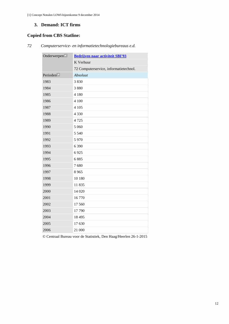
recover and supply continues to grow. To focus on technological development, we have looked for an
index of ICT development. Changes in information and communication technology are generally
recognised as the key drivers of structural changes in labour demand. Figure 3 also graphs the index of
the number of computer service and information technology agencies13
. Such firms barely existed
during the 1960’s and 1970’s, but their number exploded after the mid-1990’s. This suggests that it is
not a shift towards knowledge-intensive industries but a shift towards knowledge-intensive production
across the board that explains why a shifting supply curve has been overtaken by an even faster
shifting demand curve. The interpretation of an economy-wide increase in knowledge intensity
triggered by economy-wide application of new ICT technology matches simple day-to-day
observations as well as results in the international literature. It is also in line with results on
polarisation in the Dutch labour market as reported by Smits and De Vries (2015)14
. They find that
between 1996 and 2011, polarisation has increased in the sense that the share of low-pay jobs and the
share of high-pay jobs have both increased while the share of middle-pay jobs has decreased. The
interpretation is that computerisation can take over cognitive routine jobs in the middle segment. Low-
pay jobs, often involving non-cognitive manual routine jobs (like personal services) and high pay jobs,
involving cognitive non-routine jobs are less easily substituted by computerisation. The polarisation is
not due to a shift of employment among four main industrial sectors (agriculture, manufacturing,
commercial services and non-commercial serviceses), but operates within each sector. Unfortunately,
developments before 1996 have not been measured.
5. International comparison
10
J. Tinbergen (1975), Income distribution, Amsterdam: North Holland 11
Bron: HOT (1960-1990); CBS Statline (2001, 2010). 12
Bron: CBS Statline, Werkzame Beroepsbevolking; vergrijzing per bedrijfstak SBI 2008 (dd 17 maart 2014) en Statistisch
Zakboek 1964. 13
Bron: CBS Statline, Bedrijven naar activiteit SBI 93, K 72 14
W. Smits and J. de Vries (2105), Toenemende polarisatie op de Nederlandse arbeidsmarkt, Economisch-Statistische
Berichten 100 (4701, January 8, 24-25

[1] Concept Notulen LOWI-bijeenkomst 9 december 2014
7
Montenegro and Patrinos (2014) estimated rates of return for 139 countries using 819 household
surveys standardised for maximum comparability. The international annual mean shows a gradual
decline from the early 1980’s to around 2000 and stabilisation since then. However, it is hard to tell
how important composition effects are, as the means have not been calculated for a constant set of
countries15
.
Heckman, Lochner and Todd (2005) present estimates of the same standard Mincer earnings function
as we use, on U.S. Census data spanning the years 1940-1990. For white men, the return to education
is remarkably constant across five decades: 12.5, 11, 11, 12, 10 and 13 percent. Still, the last three
values, relating to 1970, 1980 and 1990, indicate a U-shaped pattern as observed for The Netherlands
and the increase between 1980 and 1990, by 30%, is substantial. For black men, the estimated return
increases monotonically, from 9 to 15 percent.
Harmon, Walker and Westergaard-Nielsen (2001, p 16) classify results from more than 1000 studies
(!) on Europe and the United States. Their graph shows a similar U- shaped pattern as we report here: a
marked decline from the 1960’s to the 1970’s, a further decline to the 1980’s and then recovery in the
1990’s.
6. Further explanations
While the supply and demand framework is an obvious start for an economic analysis of changes in
the structure of wages, it is equally obvious that we should not be blind to its limitations. Of course,
there is a long list of factors that may explain changes in the rate of return to education. However, we
have a specific focus on a broad feature of the developments, the U-shaped pattern observed over 5
decades. International evidence seems to confirm that this is a global development and this calls for
considering factors that operate worldwide. The simple supply and demand framework seems to match
this global development quite well. Growing participation in higher education is a world wide
development, interestingly enough precisely in the period we cover. As Shofer and Meyer (2005, p 3)16
note: :”Participation in higher education has been growing at high rates in virtually every country in
the world…..The bulk of the growth occurred after 1960, in just the last four decades.” Similarly, the
ICT revolution is a global phenomenon. It would be a broad and bold step to suggest that the race
between supply and demand, or education and technology, has developed at the same page
everywhere. Acemoglu and Autor (2012)17
, in their review of Goldin and Katz’s book that squarely
adopts the Tinbergen race as their key frame of analysis, agree that that the model does a good job in
explaining the development of the college/high school wage premium during the twentieth century. In
the US, the increased college premium in recent decades is not ascribed to speeding up of
technological develepment, but of slowing down of the growth in college participation. But the key
implication is that Tinbergen’s race model is a very fruitful approach.
A little reflection suggests that other, specific Dutch potential explanations probably will not carry
much weight in undermining our interpretation of the observed time profile. One might think that the
business cycle has some influence: the bottom of the U-shape coincides with high unemployment and
the modest decline in rates of return in recent years may be related to the recession that developed after
2008. In fact however, the relationship between rate of return and the business cycle is poorly
15
Inspection of time series for separate countries shows a variety of patterns and certainly no dominant U-shape. But for
several countries from EUROSTAT which enter the sample at the end of the period (around 2004), they usually have low
returns. This private communication from Harry Patrinos is gratefully acknowledged. 16
E. Shofer and J. Meyer (2011), The World-Wide Expansion of Higher Education, Stanford Univerity, CDDRL Working
0Papers no 32 17
D. Acemoglu and D. Autor (2012), What Does Human Capital Do? A Review of Goldin and Katz's The Race between
Education and Technology, Journal of Economic Literature, 50(2), 426-63.
[1] Concept Notulen LOWI-bijeenkomst 9 december 2014
8
known18
. Labour market institutions may have an impact on the wage structure as the relative
bargaining power of educational groups may shift over time. However, there have not been significant
changes in the system of wage bargaining; union membership rates have fluctuated, but coverage by
collective bargaining has been fairly constant. Socio-economic policies may have some effect, as
social protection at the bottom (minimum wages, unemployment and disability entitlements and
benefits) has weakened after the 1980s19
: less policy support for the lower wages may increase the rate
of return. The schooling system has been restructured, with softening the rigid selection of pupils right
after grade school but this was precisely motivated by a desire to facilitate more participation in
advanced education: it would merely help to explain the increased supply of higher educated labour.
While each of these factors may have an impact on the wage structure by education, whether
compressing or elongating, it is unclear a priori how their interaction would precisely generate the
observed U-shaped profile of returns.
A deeper analysis would certainly be interesting. Shifting demand curves can be related to changes in
the nature of job tasks and in job requirements, adding the dynamic perspective to an analysis as in
Hartog (1980)20
, in the vein of Autor, Levy and Murnane (2003)21
. The notion of shifting supply
curves can be backed up by a more detailed analysis of a changing differentiaton of the labour force by
abilities, skills and personality, Horizontal differentiaton of job requirements and types of education
can also enrich the picture. It would be interesting, for example, to trace the effects of technological
change and distinguish primary effects from spill-overs to jbs with less scope for productivity increase
(like teaching or live entertainment). But these would all be additional analyses rather than alternative
explanations. Essentially, the race between shifting supply and demand curves seems an excellent
starting point for understanding the U – shaped time profiles of the Mincerian rate of return to
education.
7. Can we trust Mincer rates of return?
In a much more extensive and profound analysis than ours of 50 years of Mincer equations for men in
the US, Heckman, Lochner and Todd (2005)22
quantify limitations of Mincer estimates of the rate of
return. Statistical tests show that separability of schooling and experience does not hold: profiles differ
by education. Calculations of internal rates of return from estimated earnings functions allowing for
these interactions and giving up linearity in the schooling effect show large variations in the rates of
return to sequential steps in schooling careers, thus rejecting the imposition of constant marginal
returns to years of schooling. Not surprisingly, a single schooling coefficient can hide large variation.
In 1940, the single Mincer coefficient for white men is 12.5 percent, while estimating marginal returns
for sequential steps of two additional schooling years each, from 6 to 16, leads to the series 12, 14, 24,
8 and 15 percent; in 1990, the linear Mincer return is 13 percent, while the step series is 19, 19, 47, 8
and 12 percent. There are also large and variable gaps among internal rates of return calculated from
estimated Mincer equations or from observed mean earning by schooling and experience cells. The
effect of including tuition cost and taxes on men’s return to schooling is actually rather mild; the
largest reductions relate to the highest level of education, in particular for black men.
18
M. Corliss, P. Lewis and A. Daly (2013), The Rate of Return to Higher Education Over the Business Cycle, Australian
Journal of Labour Economics, 16 (2), 219 – 236. 19
ESB Dossier Activerende Sociale Zekerheid, Economisch-Statistische Berichten, 2015 (47065), 26 maart 20
J. Hartog (1980), Earnings and capability requirements, Review of Economics and Statistics, LXII (2), pp. 230-240 21
D. Autor, F. Levy and R. Murnane (2003), The Skill Content of Recent Technological Change: An Empirical
Exploration, The Quarterly Journal of Economics, 118(4), 1279-1333. 22
J.Heckman, L. Lochner and P. Todd (2005), Earnings Functions, Rates of Return and Treatment Effects: The Mincer
Equation and Beyond, IZA Discussion Paper 1700
[1] Concept Notulen LOWI-bijeenkomst 9 december 2014
9
As noted, OLS Mincer estimates cannot be taken at face value as measuring causal effects. But in
1999, David Card concluded from a survey of IV studies that “the average (or average marginal)
return to education in a given population is not much below the estimate that emerges from a simple
cross-section regression of earnings on education. The “best avaliable”evidence …..suggest a small
upward bias (on the order of 10%) in the simple OLS estimates” (Card, 1999, p 1855)23
. Card suggests
that the ability bias is modest and emphasises that IV corrections are sensitive to the type of
instruments used. Rates of return to education are heterogeneous, and through their choice of
instruments, IV corrections target different segments of the distribution. Heckman, Lochner and Todd
(2005) are very critical on the value of IV estimates, arguing that instruments are mostly very weak.
For our purpose, the key question is to what extent endogeneity bias is constant over time. As far as we
know, there is only one study that compares a time series of OLS estimates with a time series of IV
estimates using the same instruments in each year. Sousa, Portega and Sa (2015) 24
use quarter of birth
as instrument to estimate returns to schooling in Portugal for each year from 1986 to 2009. Not only
the level differs among OLS and IV, but trends also differ. Taber (2001)25
analyses the rise in the
college premium in the US from early to late 1980s’ and concludes from IV, Heckman two-step and
structural dynamic programming modelling that the causal effect of college attendence has not
changed but that returns to unobserved ability have increased (the returns to observed ability, i.e.
AFQT score, has not changed); estimation (and interpretation) of the dynamic programming model is
marred by a problem of multiple optima. Taber’s conclusion fits in with the the dominant view of ythe
time, but Cawley, Heckman and Vytlacil (1998)26
do not agree that the increase in the college
premium in the US would be due to an increase in the return to ability. They show that the result is not
robust and point to two serious identification problems: the effects of time and age cannot be
disentangled, and strong sorting of education by ability leaves most education-ability combinations
unobserved. They reject the linear models that have been applied and conclude from their own non-
parametric estimates that in the mid-80’s the college premium has increased for young white males of
high ability, but that little can be said for other ability groups.
8. Conclusion
After assessing comparability of a number of studies on the Mincer earnings function in the
Netherlands, we can confidently draw two clear conclusions, both for men and for women: over a
period of five decades since 1960, the rate of return to education has followed a U shaped pattern with
bottom in the mid-1980’s, while the slopes of earnings-experience profiles have not changed. The U-
shape can be explained with Tinbergen’s race between supply and demand: initially the growth of
participation in higher education outpaced the growth in demand, while later the ICT revolution
pushed out the demand curve faster than the supply curve. This history is similar to international
developments.
In spite of its elegant theoretical underpinning, we should not forget that essentially, the Mincer rate of
return is a convenient summary statistic of the wage structure by level of education. Log-linearity in
23
D. Card (1999), The causal effect of education on earnings, in O. Ashenfelter and D. Card, Handbook of Labor
Economics, volume 3A, Amsterdam: North-Holland 24
S. Sousa, M. Portela and C. Sa (2015), Characterization of returns to education in Portugal: 1986-2009, Working Paper
Catolica Lisbon School of Economics and Business 25
C. Taber (2001), The Rising College Premium in the Eighties: Return to College or Return to Unobserved Ability? , The
Review of Economic Studies, 68 (3), 665-691 26
J. Cawley, J. Heckman and E. Vytlacil (1998), Cognitive ability and the rising return to education, NBER Working Paper
6388

[1] Concept Notulen LOWI-bijeenkomst 9 december 2014
10
years of schooling is a simplification that hides miuch variation. On changes in the causal effect of
education on wages we cannot draw firm conclusions

[1] Concept Notulen LOWI-bijeenkomst 9 december 2014
11
Data Appendix
1. Supply: Share of tertiary educated in the labour force
1960 1975 1979 1990 2001 2010
Male 4.0 10.8 13.6 20.0 25.5 33.2
Female 1.0 9.1 11.9 19.8 33.2 35.0
Source: HOT (1960-1990); CBS Statline (2001, 2010)
2. Supply: Aggregate share of tertiary educated if shares within industries were constant
Share of higher educated in the labour force if the share of higher educated within industries is held
constant at the level in 2001, and employment across industries shifts over time as observed
1960 1971 1975 1979 1983 1987 1991 1995 1999 2003 2007 2011 2012
18.20 18.69 21.29 22.11 23.75 24.25 24.40 24.97 25.26 26.21 26.66 27.09 27.02
Source 1971-2012
Share higher educated in labour force by industry 2001: CBS Statline, Werkzame Beroepsbevolking;
vergrijzing per bedrijfstak SBI 2008 (dd 17 maart 2014), Totaal M/V, 15 +, totaal herkomstgroepering,
totaal werkzame beroepsbevolking
Share labour force by industry: 1971-2012: idem, idem, SBI 93
Share labour force by industry 1960: Statistisch Zakboek 1964, H74, p 40
Added: werknemers Gemeente (H78, p 43), Rijk (H77, p 44) voor Sector Overheid, afgezonderd van
“Overige dienstverlening”; Restant “Overige dienstverlening” samengevoegd met “Huiselijke
diensten”.
Share higher educated added up to Aggregate 1960, weight of subgroups 1971 :
Handel, Bank Verzekering = G+J
Overig= H+K+M+N+O
Datasources: CBS statline
Labour force by industry: Werkzame beroepsbevolking; vergrijzing per bedrijfstak SBI ‘93;
verslagperiode 1971-2013; 14 maart 2014
Share higher educated: Werkzame beroepsbevolking; vergrijzing per bedrijfstak SBI 2008; 14 maart
2014
[1] Concept Notulen LOWI-bijeenkomst 9 december 2014
12
3. Demand: ICT firms
Copied from CBS Statline:
72 Computerservice- en informatietechnologiebureaus e.d.
Onderwerpen Bedrijven naar activiteit SBI'93
K Verhuur
72 Computerservice, informatietechnol.
Perioden Absoluut
1983 3 830
1984 3 880
1985 4 180
1986 4 100
1987 4 105
1988 4 330
1989 4 725
1990 5 060
1991 5 540
1992 5 970
1993 6 390
1994 6 925
1995 6 885
1996 7 680
1997 8 965
1998 10 180
1999 11 835
2000 14 020
2001 16 770
2002 17 560
2003 17 790
2004 18 495
2005 17 630
2006 21 000
© Centraal Bureau voor de Statistiek, Den Haag/Heerlen 26-1-2015
[1] Concept Notulen LOWI-bijeenkomst 9 december 2014
13
Table 1. Mincer rates of return: effects of differences in data surces
HOT SOH JW GH
m m m v m v m v
1979 LS gh25+ 8.9
1979 LS gh 6.4 6.0
1982 OSA gh25+ 7.3
1982 OSA gh 7.8
1982 OSA nh 7.4
1985 LS gh25+ 7.2
1985 LS gh 5.2 5.0
1985 OSA nh 5.0
1988 OSA gh25+ 5.9
1988 OSA gh 6.1
1988 OSA nh 5.5 6.1 6.0
1989 LS gh25+ 7.3
1989 LS gh 5.0 4.5
1996 OSA nh 6.3 5.1
1996 OSA gh 7.5 5.6
1996 OSA ny 6.1 6.8
1996 OSA gy 7.3 7.8
1996 LS gh 6.1 6.2
2002 CBSp gh 8.0 7.2
2002 LS gh 7.5 7.5
g=gross, n=net; h=hourly wage, y=annual wage ; 25+=25 years and older; m=men, v=women
LS CBS Loonstruktuuronderzoek (Wage structure Survey)
CBSp CBS Panel Project

[1] Concept Notulen LOWI-bijeenkomst 9 december 2014
14
Table 2. Mincer rates of return: time series
HOT SOH JW GH LO
m m m v m v m v m v
1962 LS ghw25+ 11.0
1965 LS ghw25+ 10.2
1972 LS ghw25+ 9.3
1979 LS gh25+ 8.9
1979 LS gh 6.4 6.0
1982 OSA gh25+ 7.3
1982 OSA gh 7.8
1982 OSA nh 7.4
1985 LS gh25+ 7.2
1985 LS gh 5.2 5.0
1985 OSA nh 5.0
1986 OSA nh 4.8 5.8 6.2
1988 OSA gh25+ 5.9
1988 OSA gh 6.1
1988 OSA nh 5.5 6.1 6.0
1989 LS gh25+ 7.3
1989 LS gh 5.0 4.5
1990 OSA nh 5.4 6.0
1992 OSA nh 5.6 5.3
1994 OSA nh 6.3 5.7
1994 IALS gh 5.7 5.7
1996 OSA nh 6.3 5.1
1996 OSA gh 7.5 5.6
1996 OSA ny 6.1 6.8
1996 OSA gy 7.3 7.8
1996 LS gh 6.1 6.2
1997 LS gh 6.6 6.6
1999 NIPO gh 8.0 9.0
1999 CBSp gh 7.2 6.5
2000 CBSp gh 7.4 6.5
2001 CBSp gh 7.9 6.9
2002 CBSp gh 8.0 7.2
2002 LS gh 7.5 7.5
[1] Concept Notulen LOWI-bijeenkomst 9 december 2014
15
2003 CBSp gh 8.1 7.0
2004 CBSp gh 8.0 6.6
2005 CBSp gh 8.3 7.0
2006 CBSp gh 8.4 7.2
2007 CBSp gh 8.9 7.3
2008 CBSp gh 8.8 7.6
2009 CBSp gh 8.9 7.6
2010 CBSp gh 8.8 7.9
2011 CBSp gh 8.7 7.3
2012 CBSp gh 8.4 7.2
g=gross, n=net; h=hourly wage, y=annual wage; w=employees (white collar); 25+=25 yeas and older;
m=male, v=female
LS CBS Loonstruktuuronderzoek
CBSp CBS Panel Project
NIPO, IALS see text on LO

[1] Concept Notulen LOWI-bijeenkomst 9 december 2014
16
Table 3. Wage growth over the first 10 years ( 2 310 100 ).
HOT SOH JW GH
m m m v m v m v
1962 LS ghw25+ .513
1965 LS ghw25+ .490
1972 LS ghw25+ .480
1979 LS gh25+ .326
1979 LS gh .636 .593
1982 OSA gh25+ .299
1982 OSA gh .430
1982 OSA nh .350
1985 LS gh25+ .328
1985 LS gh .707 .744
1985 OSA nh .340
1986 OSA nh .280 .393 .367
1988 OSA gh25+ .300
1988 OSA gh ,370
1988 OSA nh .350 .421 .372
1989 LS gh25+ .344
1989 LS gh .727 .731
1990 OSA nh .449 .341
1992 OSA nh .397 .282
1994 OSA nh .448 .313
1995
1996 OSA nh .443 .344
1996 OSA gh .488 .382
1996 OSA ny .433 .184
1996 OSA gy .477 .226
1996 LS gh .731 .709
1997 LS gh .789 .736
1999 CBSp gh .237 .269
2000 CBSp gh .234 .251
2001 CBSp gh .220 .255
2002 CBSp gh .200 .240
2002 LS gh .723 .596
2003 CBSp gh .205 .243
2004 CBSp gh .207 .243

[1] Concept Notulen LOWI-bijeenkomst 9 december 2014
17
2005 CBSp gh .214 .239
2006 CBSp gh .207 .243
2007 CBSp gh .207 .245
2008 CBSp gh .215 .222
2009 CBSp gh .196 .198
2010 CBSp gh .193 .199
2011 CBSp gh .212 .189
2012 CBSp gh .188 .206
g=gross, n=net;h=hourly, y=annual; w=white collar only; 25+=25 and older
LS CBS Loonstruktuuronderzoek
CBSp CBS Panel Project
[1] Concept Notulen LOWI-bijeenkomst 9 december 2014
18
Figure 1a: Mincer returns to schooling: men
Figure 1b: Mincer returns to schooling: women
46
81
01
2
retu
rn
1962 1972 1982 1992 2002 2012year
HOT25 HOT
JW GH
45
67
8
retu
rn
1962 1972 1982 1992 2002 2012year
JW GH

[1] Concept Notulen LOWI-bijeenkomst 9 december 2014
19
Figure 2a. Predicted wage growth during the first 10 years: men
Figure 2b. Predicted wage growth during the first 10 years: women
.2.4
.6.8
wag
e g
row
th
1980 1990 2000 2010year
HOT25 HOT
SOH JW
GH
.2.4
.6.8
wag
e g
row
th
1980 1990 2000 2010year
SOH JW
GH

[1] Concept Notulen LOWI-bijeenkomst 9 december 2014
20
Figure 3: Supply and demand higher educated labour
010
20
30
40
% o
f m
en that is
hig
hly
educate
d
1960 1970 1980 1990 2000 2010year
010
20
30
40
% o
f w
om
en that is
hig
hly
educate
d
1960 1970 1980 1990 2000 2010year
18
20
22
24
26
28
% h
ighly
educate
d in industr
y
1960 1970 1980 1990 2000 2010year
5000
10000
15000
20000
num
ber
of IC
T a
gencie
s
1960 1970 1980 1990 2000 2010year