POTENTIAL UNEMPLOYMENT INSURANCE DURATION AND LABOR SUPPLY: THE INDIVIDUAL AND MARKET-LEVEL RESPONSE TO A BENEFIT CUT*

April 2017

Andrew C. Johnston

University of California, Merced

Alexandre Mas Princeton University and NBER

ABSTRACT

We examine how a 16-week cut in potential unemployment insurance (UI) duration in Missouri affected search behavior of UI recipients and the aggregate labor market. Using a regression discontinuity design (RDD), we estimate a marginal effect of maximum duration on UI and nonemployment spells of approximately 0.45 and 0.25 respectively. We use the RDD estimates to simulate the unemployment rate assuming no market-level externalities. The simulated response, which implies almost a one percentage point decline in the unemployment rate, closely approximates the estimated change in the unemployment rate following the benefit cut. This finding suggests that, even in a period of high unemployment, the labor market absorbed this influx of workers without crowding-out other jobseekers.

*We are grateful to David Card, Mark Duggan, Henry Farber, Erik Hurst, Robert Jensen, Pauline Leung, Olivia S. Mitchell, Kurt Mitman, Ulrich Müller, Zhuan Pei, Jesse Rothstein, Johannes Schmieder, Steven Woodbury, and workshop participants at the ABL conference, Georgetown, New York Federal Reserve, Princeton University, UC Berkeley, The Wharton School, Universitat Autonoma de Barcelona, University Carlos III, and University of Wisconsin. Elijah De La Campa, Kevin DeLuca, Disa Hynsjo, Samsun Knight, Dan Van Deusen, and Sophie Zhu provided excellent research assistance.

2

I. INTRODUCTION How do recipients respond to the maximum duration of unemployment insurance (UI)

benefits and how do these responses affect the broader labor market? These questions are important

for evaluating UI programs and labor-market performance over the business cycle. A large

literature has estimated the relationship between maximum UI duration and the behavior of UI

recipients and some researchers have hypothesized that extended benefits may have contributed to

slow job-market recoveries (Mitman and Rabinovich 2014). However, evidence of the relationship

between potential UI duration and labor-market outcomes is thin, especially after the mid-1990s

in the United States. Additionally, if there are general-equilibrium effects or spillovers, the

aggregate effects of these policies may differ substantially from those implied by the micro

response, as would be the case if job searching among UI recipients crowded out other jobseekers.

With a few notable exceptions (Levine 1993, Valletta 2014, Marinescu 2014, and Lalive, Landais,

and Zweimuller 2015), we know relatively little about the relationship between the micro and

macro responses to UI extensions.1

Using newly available administrative data with regression discontinuity and difference-in-

differences designs we study the micro and macro effects of a large cut in Missouri’s benefit

duration that occurred in 2011. Following the 2007–2009 recession, eight U.S. states reduced

regular UI durations in response to diminished reserves in state UI trust funds and a changing

political environment. While there is a precedent for cutting UI benefit generosity, to our

knowledge, this was the first time states cut UI benefit durations. These states (Arkansas, Florida,

1 There is also a literature testing for externalities from job search assistance programs in Western Europe. These include Blundell et al. (2004), Crépon et al. (2013), Ferracci, Jolivet, and van den Berg (2010), and Gautier et al. (2012). Davidson and Woodbury (1993) consider displacement effects from reemployment bonuses in the United States. General-equilibrium estimates in Hagedorn et al. (2013) and Hagedorn, Manovskii, and Mitman (2015) are also related to tests for the presence of externalities.

3

Georgia, Kansas, North Carolina, Missouri, Michigan, and South Carolina) cut the duration of UI

benefits to below 26 weeks, the duration that had been the standard in place for over half a century.2

We examine the effect of UI benefit duration on the duration of UI receipt, the length of

nonemployment, wages, and the aggregate unemployment rate by evaluating the dramatic cut in

UI benefit weeks implemented in Missouri in April 2011. This reduction resulted in dislocated

workers receiving up to 16 fewer weeks of UI eligibility than they would have received if they had

applied previously, since the six-week state cut triggered a ten-week cut in federal benefits from

the Emergency Unemployment Compensation (EUC) program.3 The policy change was sudden

and unanticipated; only five days passed between when the legislation was first proposed and when

the law applied to new UI claimants, giving almost no opportunity for the unemployed to shift the

timing of their claims.

We use rich unemployment insurance administrative program data and wage records from

Missouri with a regression discontinuity design (RDD) to estimate the effects of this policy. The

running variable is calendar time and the threshold of interest is the exact week the law was enacted

and implemented.4 The administrative data we use not only allow us to measure UI receipt but also

re-entry into employment and wages which has not been possible in the vast majority of papers

investigating UI in the United States, particularly in recent years.

Our findings indicate economically and statistically significant higher rates of exit from UI

for claimants who are subject to the shorter benefit duration than those with the longer duration at

the cutoff resulting in an estimated sensitivity of unemployment duration to potential UI duration

2 In 2010, all states had a maximum duration of benefit eligibility of at least 26 weeks. 3 The maximum UI duration was cut by 16 weeks for UI recipients who previously had been eligible to receive extended benefits provided by the EUC program in addition to the 26 weeks of regular state UI. 4 More precisely, this is an interrupted time-series design, but we use RDD and refer to the design as an RDD throughout.

4

that is at the upper end of the literature. As found in Card, Chetty, and Weber (2007), Schmieder,

von Wachter, and Bender (2012), as well as Le Barbanchon (2012), we find evidence that some

UI recipients are forward-looking. For example, UI recipients subject to the benefit cuts had 57

weeks of eligibility, but were 7.5 percentage points less likely to receive UI by week 20 of their

spell, from a base of 56 percent. We estimate that a one-month reduction of UI duration reduces

UI receipt an average of 1.8 weeks and that approximately 45 percent of this change is through

earlier exits prior to benefit exhaustion.

Analysis of earnings records for all legally employed Missouri workers indicates that those

exiting UI early enter employment. The estimates imply that a one-month cut in potential duration

resulted in a reduction of nonemployment duration of approximately 1.1 weeks, suggesting the

benefit cut increased job search. However, we find more limited effects of shorter benefits on the

long-term unemployed. In particular, we find no evidence that lower potential duration leads to

higher employment after UI exhaustion.

Similar to the findings of some other studies (Van Ours and Vodopivec, 2005; Card,

Chetty, and Weber, 2007; Lalive, 2007; Lindner and Reizer, 2016) we find no significant

difference in reemployment earnings, conditional on employment, relative to the comparison

group, which suggests that those induced to exit unemployment earlier are not penalized with

lower wages.

The effects of extended UI on other job seekers is theoretically ambiguous. If there is job

rationing, which can arise in search models with diminishing returns to labor and sticky wages

(Michaillat 2012), increased search effort leads to negative externalities on other workers.

However, there are no externalities in models with constant marginal returns to labor and perfectly

elastic labor demand (Landais, Michaillat, and Saez 2010; Hall 2005). In models of Nash

5

bargaining (such as Pissarides 2000), the macro elasticity of UI benefits is larger than the micro

elasticity as a result of a “wage externality.”

To assess spillovers, we calculate the change in the predicted path of the unemployment

rate from the policy using the shift in the survivor function estimated from the RDD and the flow

of initial UI claims. In the simulation, we assume that jobseekers are not displaced by additional

search effort from UI recipients who were exposed to the cut. We compare this predicted path to

the actual path of the unemployment rate from a differences-in-differences (DiD) estimate of the

cut. We find that the simulated and estimated paths of the macro effect closely match. The

predicted and estimated paths are close in levels and follow a similar kinked pattern, peaking at

almost a one percentage point drop in the state unemployment rate, suggesting that the labor market

absorbed jobseekers without displacement, even though the unemployment rate was high (8.6

percent) at the time of the cut. The findings are more consistent with a labor market characterized

by a flat labor demand curve in Landais, Michaillat, and Saez (2010).

Our study also speaks to the labor-market effects of UI extensions during the Great

Recession. During this period, UI benefits increased from the near-universal length of 26 weeks

to up to 99 weeks in some states. Subsequently, declining unemployment led to reductions in

extended benefits, and benefit duration largely returned to pre-recession levels following the

expiration of the federal EUC program in December 2013. The labor-market effects from these

changes in benefit duration are a central question for labor-market policy and have been the focus

of several studies. Notably, recent papers studying this period in the United States have used state-

level variation in benefit lengths to estimate the effects of UI potential duration over the 2007

recession period and its aftermath. The findings from these studies are mixed. Rothstein (2011),

Farber and Valletta (2013), and Farber, Rothstein, and Valletta (2015) find limited effects of the

6

UI extensions on job finding. Hagedorn et al. (2013) find small effects on jobseekers but large

macro effects on wages, job vacancies, labor-force participation, and employment. Hagedorn et al.

(2015) provide evidence of very large effects of cuts in UI duration on unemployment. Our paper

contributes to this literature by using a design-based approach with administrative micro data

covering UI receipt, employment, and wages to study the labor-market effects of changes in

maximum duration in this period. While we find little evidence of moral hazard for the long-term

unemployed who exhaust their benefits, we identify a large response to the benefit cut for a subset

of participants prior to exhaustion.

II. INSTITUTIONAL BACKGROUND

In the United States, UI is administered by state governments but is overseen and regulated

by the federal government. Before 2011, eligible laid-off workers received up to 26 weeks of

regular UI benefits if they were not reemployed before their benefits were exhausted. During

periods of unusually high unemployment, state and federal governments have extended potential

benefit duration to support the long-term unemployed after regular benefits are exhausted. In the

2007–2009 recession, two programs provided these extended benefits: the Extended Benefit (EB)

program and the Emergency Unemployment Compensation (EUC) program.

EB is a permanent federal program that provides extended benefits to unemployed workers

who exhaust their regular state benefits in states with high unemployment. Until recently, the

federal government split the cost of EB with state governments. Through the Recovery Act passed

in February 2009, Congress temporarily suspended cost sharing and the federal government bore

all the cost of EB through December 2013. EB extended benefits are triggered as a function of a

state’s total and insured unemployment rate, and triggering thresholds vary by state. When the

7

federal government took on all the costs of EB, Missouri temporarily enacted legislation to

implement an additional trigger that would increase EB duration from 13 to 20 weeks.5

Congress occasionally extends unemployment duration through additional legislation

when unemployment is high. During the period of the 2007–2009 recession, the EUC program

was active from June 2008 through December 2013. In the version in place at the time of the

Missouri policy change, federal benefits provided longer extensions for states with higher rates of

insured unemployment.6

The benefit cut in Missouri was the byproduct of a Republican filibuster, led by four

lawmakers in the Missouri State Senate who objected to legislation that would accept federal

money to extend UI benefits under the EB program. The bill would have allowed for the

continuation of 20 additional weeks of benefits to unemployed workers who exhausted their EUC

and regular benefits at no cost to Missouri.7 The extension had already passed the Missouri State

House by a margin of 123 to 14. The first news reports of the filibuster were published March 4,

2011 (Wing 2011). On April 6, a report indicated that the lawmakers had agreed to end their

filibuster, though the article did not specify terms (Associated Press 2011). On April 8, the St.

Louis Post Dispatch published the first article detailing the possible compromise. Under the

compromise, regular benefits would be cut from 26 to 20 weeks in exchange for Missouri accepting

5 If the total unemployment rate (TUR) was at least 8 percent and 110 percent of the TUR for the same three-month period in either of the two previous years, the duration of EB would increase from 13 to 20 weeks (http://www.cbpp.org/cms/index.cfm?fa=view&id=1466). 6 At that time EUC, had four “tiers”: tier 1 = 20 additional weeks, tier 2 = 14 additional weeks, tier 3 = 13 additional weeks, and tier 4 = 6 additional weeks. To move into a new tier, recipients had to exhaust the previous tier and the next tier had to be available to state residents. The availability of tiers depended on whether the three month average of the seasonally adjusted state unemployment rate exceeded a threshold set for that tier. At the time of the policy change, Missouri recipients were eligible for all four tiers. However, recipients who claimed UI around the time of the policy change in April 2011 were only ever able to claim the first three tiers because the state unemployment rate fell below the tier 4 threshold in February 2012, prior to tier 3 exhaustion. 7 The lawmakers leading the filibuster argued that accepting these funds would increase the federal deficit unnecessarily.

8

federal dollars and maintaining EB benefits for the long-term unemployed (Young 2011). In effect,

the agreement traded-off longer UI durations in the short-run (for the long-term unemployed) in

exchange for shorter UI durations in the long run. We found no press reports prior to April 8

regarding the possibility of cutting the duration of regular benefits as a possible compromise for

the filibuster. This legislation appears to have been unanticipated. On April 13, the Missouri House

of Representatives passed the bill, which the governor signed into law on the same day (Selway

2011). All new claims submitted after that date were subject to abbreviated benefits (Mannies

2011).

Federal regulations calculate EUC weeks eligible in proportion to regular state UI benefits.

Thus, the cut in regular state UI benefits triggered an additional ten-week reduction in EUC, and

the maximum UI duration fell from 73 weeks for claimants approved by April 13, to 57 weeks for

claimants approved afterwards resulting in a total change in potential duration of 16 weeks. EB

did not materially affect new claimants at this time (with or without the benefit cut) because EB

phased out by the time they were eligible to receive these benefits.

The change in potential UI duration was the only change in Missouri’s UI system in the

legislation. We corresponded with Missouri UI program administrators who told us that there were

no changes in the administration of the program, including search requirements or communications

with UI recipients. For example, they did not send additional notices informing UI recipients

affected by the policy change.

For convenience, we label recipients applying for UI after the policy change the “treatment

group” and recipients applying before the policy change the “control group.”

9

III. DATA

Our analysis utilizes administrative data from the state of Missouri covering workers,

firms, and UI recipients from 2003 to 2013. We use three data files for the analysis. The first is a

worker-wage file detailing quarterly earnings for each worker with unique (but de-identified)

employee and employer IDs. The second is an unemployment claims file that contains the same

worker and employer IDs as the wage file. For each claim, we observe the date the claim was filed,

the weekly benefit amount, the maximum benefit amount over the entire claim, the dates weekly

benefits were issued, the wage history used to calculate benefits and duration, and the benefit

regime (i.e., regular benefits, EB, or EUC). For every claim, we link the records for regular

benefits, EB, and EUC claims to construct a single continuous history associated with each claim.

The third dataset reports a limited set of employer characteristics including detailed industry

categories. The raw data contains 1,635,993 initial UI claims from 2003 to 2013 and 184,191

claims in 2011. We remove claims ineligible for UI, including unemployed workers who were

fired for cause or quit voluntarily, observations with missing claim types (regular, EB, or EUC) or

missing base-period earnings, and EB or EUC claims that could not be traced to an initial regular

claim. To aid in interpreting the effects, we also limit the sample to those workers who, based on

their earnings histories, would have been eligible for the full 26 weeks of regular UI benefits

without the policy change. Specifically, the formula for maximum potential duration of regular

benefits is:

Regular Potential Duration = min !,#

$

%

&

where E is a measure of total base period earnings, B is the average weekly benefit, and X is 26

weeks on or before April 13, 2011 and 20 weeks after this date. Because we want to focus on

workers who are affected by the cut in maximum duration we select recipients for whom #$&≥ 26.

10

This procedure does not induce any mechanical change in the characteristics of workers across the

policy change threshold. These “full eligibility” claimants represent 72 percent of all claimants in

2011 and 67 percent of all claimants for the entire 2003–2013 period. After these screens, we have

1,064,652 claims over the 2003–2013 period and 127,710 claims in 2011.

Descriptive statistics for the administrative data appear in Table 1. Column (1) reports

summary statistics for the full 2003–2011 period and column (2) for 2011. The average weekly

benefit in 2011 in the sample was $260. UI recipients eligible for the maximum benefit duration

had an average of 14.5 quarters of tenure in their previous employer and their earnings in the last

complete quarter of employment prior to collecting UI benefits was $8,259. Earnings in the first

complete quarter of employment after the UI spell average $7,240. On average, recipients claiming

benefits in 2011 received 29.3 weeks of unemployment benefits.

For the aggregate analysis, we use data from the Local Area Unemployment Statistics

(LAUS) program of the Bureau of Labor Statistics. For outcomes we use the state-by-calendar

month unemployment rate, the natural log of number of unemployed, and the labor force

participation rate. We deseasonalize these variables by regressing each outcome on state × month

dummies over the 2001–2005 period and then deviating each outcome in 2005–2013 from the

predicted value of this regression. We also use these variables derived from the Current Population

Survey (CPS) to assess robustness.

IV. EMPIRICAL DESIGN

To identify the causal effect of longer UI duration, we utilize the discrete change in the

maximum UI duration resulting from a rapid and unexpected policy change: claimants who applied

just before April 13, 2011 were eligible for 73 weeks of benefits and those who applied after were

eligible for 57 weeks. We use this discontinuity to compare similar displaced workers entering the

11

same labor market who experienced very different UI benefit durations. This quasi-experiment

implicitly controls for labor-market conditions that may be affected by the reform.

We model the outcome variable () as a continuous function of the running variable, the

claim week, and estimate the outcome discontinuity that occurs at the threshold, the date of the

policy change:

(1) () = +,) + . /) − /1+ 2),

where /) is the calendar week of the UI claim for person i, /1 is the week of the policy change, and

,) equals one if worker i applied after the policy change and zero if she applied before.8 Thus,

. /) − /1 is a continuous function of the running variable which captures the continuous

relationship between the application date and the outcome of interest. Because we control flexibly

for the running variable, the model can accommodate smooth seasonal and secular changes in the

labor market, allowing for unbiased estimation of the effect of the discrete policy change. To

expand on this point, the unemployment rate in Missouri began to decline in the months before the

policy was enacted. If our model is correctly specified, a smooth improvement in labor-market

conditions would be captured by the term . /) − /1 . A threat to validity would be if there was a

discrete change in the labor market from one week to the next at the time of the policy.

In practice, we first collapse the data to the claim week level and weight the observations

by the number of claims in the week, a process that yields identical point estimates to the micro

data. As shown by Lee and Card (2008), heteroskedasticity-consistent inference with collapsed

data is asymptotically equivalent to clustering on the running variable. We estimate the model

using local linear regression (Hahn, Todd, and Van der Klaauw 2001) with the Imbens and

Kalyanaraman (2012) (IK) optimal bandwidth and a triangular kernel. We consider a range of

8 We use the claim week because the data can be sparse when using the claim application calendar date, and there are days with no claims, such as administrative holidays and weekends.

12

alternative bandwidths to assess robustness, as well as estimation of a local quadratic using the

Calonico, Cattaneo, and Titiunik (2014) (CCT) optimal bandwidth.

V. DIAGNOSTICS

We begin by testing for manipulation of the running variable, which might occur if

claimants could strategically time their applications around the policy change. Figure 1 plots the

frequency distribution of the number of UI claims by week, over the 2009–2012 period. The solid

vertical line denotes the time of the policy change, and the dashed vertical lines denote the same

date in the previous years. It is evident in Figure 1 that there is a great deal of seasonality in claims,

with a large spike in claims around the new year. The policy change occurred after the large

seasonal increase, in April, and by this time claims were at moderate levels. There is no abnormal

spike in claims before the policy change, as would be the case if claimants could time their

applications for longer-lasting UI benefits. Column 1 of Table 2 formally tests for a discontinuity

in claims (as in McCrary 2008). Estimating a local quadratic model to fit the curvature in the

distribution, we find no significant discontinuity in the relative frequency of claims.9

Inspection of the frequency distribution does reveal a moderate jump in claims two weeks

after the change in policy. As we will show, this applicant cohort looks different in a number of

dimensions from recipients who applied before or after this group, and in particular they appear to

have characteristics correlated with being lower duration claimants. This outlier might be random

noise, or it might reflect a failed attempt to time claims to obtain UI before the cut. To err on the

conservative side, we remove this group from the main specifications. For reference, we also

estimate all models including this cohort.

As a second examination of design validity, we test for discontinuities in pre-determined

9 Appendix Figure 1 displays the fitted quadratic in the frequency distribution.

13

covariates of UI applicants around the policy change. Because there are numerous predetermined

variables from which we can select, we construct an index of predicted log initial UI duration using

all covariates available in the data set following the same procedure as Card et al. (2015). To

construct the index, we regress log UI duration on a fourth-order polynomial of earnings in the

quarter preceding job loss, indicators for four-digit industry, and previous job tenure quintiles.

Figure 2 plots the mean values of the covariate index over 2009–2012 by claim week. The

continuity in the index around the threshold is borne out visually, and the RDD estimate of this

predicted value at the cutoff is small and statistically insignificant (column (2) of Table 2). The

lack of evidence of sorting and differences in predetermined characteristics around the threshold

reinforces the claim that the policy change was unanticipated and difficult or impossible to game.10

V. MICRO RESULTS

In this section, we discuss the main micro results. In the following section, we perform

several robustness checks including placebo analyses, permutation tests, varying bandwidths, and

assessing the influence of seasonality.

Duration of UI Receipt

Figure 3 exhibits the mean duration of realized UI spells by application week. There is a

clear drop in the number of weeks claimed as a function of the claim week. Column (1) in Table

3 shows that the benefit reduction of 16 weeks is associated with 7.2 fewer weeks of UI benefits

claimed (s.e. = 0.82), on average.

The reduction in weeks of UI receipt is a possible combination of “mechanical” effect of

earlier exhaustion for the treatment group and pre-exhaustion UI exit. We decompose the overall

10 In Figure 2 we see that the cohort receiving claims two weeks after the duration cut has substantially lower predicted durations.

14

change in weeks of UI receipt into two parts: the part due to changes in behavior prior to exhaustion

and the part due to post-exhaustion exit. The estimated effect of treatment on unemployment

duration conditional on duration being less than 58, that is, excluding anyone exhausting, is 4.4

weeks. Because E[Duration] = E[Duration|Duration < 58] * Pr(Duration<58) +

E[Duration|Duration ≥58] * Pr(Duration≥58), and Pr(Duration<58) ≈ 0.74 in the control group,

approximately 45 percent (=100*(4.4*0.74)/7.2) of the change in the overall duration of UI receipt

comes from changes in the response to the cut before exhaustion.

Timing of UI Receipt

To examine the timing of UI receipt in greater detail, we estimate the probability that an

individual remains on UI through each of the first 73 weeks of the spell. Figure 4 presents binned

scatterplots of the probability that claimants remained on UI in weeks 20, 40, 55, and 60 as a

function of their initial claim week. The figure shows that there is a response to the cut in maximum

duration fairly early in the spell. In weeks 20, 40, and 55, before the treatment group exhausted

benefits, it can be seen visually that the duration cut is associated with a lower probability of

receipt. By week 60, the probability of remaining in UI for the treated group falls to about zero,

consistent with all remaining claimants in the treatment group exhausting their benefits, while 25

percent of the comparison group was still receiving UI at that point. In none of these series do we

see a similar break one year prior to the policy change (denoted by the dashed vertical line).

Table 3 columns (2)–(5) report the point estimates for the probability that the UI spell

lasted until weeks 20, 40, 55, and 60. The RDD estimate for UI receipt is -7.5 percentage points in

week 20, -0.09 percentage points in week 40, -0.08 percentage points in week 55, and -24

percentage points in week 60. All estimates are highly significant.

To estimate the timing of the effects over the whole period, we fit variants of equation (1)

15

where, in each specification, () is the probability that the claimant received at least T weeks of

benefits, where T spans 1 to 73. These estimates give the relative survival probabilities between

the two groups, week by week. Figure 5 plots each of the RDD estimates with the associated

confidence intervals. The figure shows that the survival function diverges between the two groups,

starting after 4 weeks into the UI spells.

Note that there is a sharp drop in the survivor rate for the treatment group in week 20 and

a similar drop for the comparison group in week 26. These drops represent individuals who did

not receive benefits beyond the regular state benefits, either because they were ineligible since the

federal government automatically enrolls the eligible, or did not enroll for other reasons.11 Because

of these drops in the survivor rate at regular benefit exhaustion date, we do not interpret the 20–26

week span because any differences over this term reflect a combination of eligibility and

behavioral effects.

Excluding this 20–26 week period, the treatment-control differences in the survivor rate

are relatively stable from week 20 of the UI spell through week 57, at which point there is a

significant drop in the relative survivor rates as the treatment group exhausts EUC benefits while

the control group continues to receive EUC benefits until week 73. The error bands in Figure 5

show that gap between the two groups are significant after week 5, and the differences remain

significant after that point. These estimates indicate claimants respond in a forward-looking way

to UI exhaustion, and much of the response to the duration cut occurs fairly early in the spell,

within the first three months.

11 It is also possible that this dip could be the result of unmatched administrative claims data. The raw administrative data has a separate record for each type of claim (regular benefits, different EUC tiers, extended benefits). We matched the records to form a continuous history. To the extent that we couldn’t match regular benefits to EUC records this pattern would emerge. However, we believe that it is unlikely that this slippage plays a major role in this pattern since the different tiers of EUC are also separate records, and we would therefore expect to see similar step patterns at all points where these transitions occur, which we do not.

16

We can use the estimated survival functions to estimate the average change in the hazard

rate. In Panel A of Figure 6 we show the level of the survival rate for the control and treatment

groups that underlie Figure 5. A point in the survivor curve for the control is the constant in the

local linear regression used to estimate a weekly estimate in Figure 5. The treatment series is the

corresponding intercept for the treatment group. The difference in these two series is Figure 5.

Panel B shows the survivor functions in logs. The slope of these functions times –1 is the hazard

rate. To compute the hazard rate, we first smooth the survivor functions separately over weeks 1–

20 and 26–57 for the treatment group and weeks 1–26 and 26–73 for the control group.12 We use

these separate segments so as to not have the function be influenced by the drop in the survivor

function due to regular UI recipients not claiming EUC. We then numerically differentiate these

smoothed functions. The derivatives times –1 are plotted in Panel C. The difference in the

estimated hazard rates are shown in Panel D.

This exercise reveals several features about the response of recipients to the cut in benefits.

As can be seen in Figure 5, there is a large response between weeks 5 and 20 of the spell, where

the hazard is approximately 0.5–1 percentage point higher in the treatment than the control.

However, the exit hazard in the treatment remains elevated after 26 weeks, something that is not

necessarily apparent when looking at raw survivor functions in Panel A. On average, the treatment

group has a 30 percent higher exit hazard than the control over the first 57 weeks of the UI spell.

This translates into a large elasticity of exit hazard with respect to the cut of 1.36.13 A second

interesting feature is that, consistent with Meyer (1990), there are spikes in the exit hazard prior to

exhaustion. This can be seen both for the treatment and control groups approaching the EUC

exhaustion weeks.

12 To smooth the series we use a kernel-weighted local polynomial smoother of degree two, and a bandwidth of 5. 13 The policy resulted in a 22% change in potential UI duration (16 weeks from a base of 73).

17

Employment

Using the quarterly wage files we can measure the employment rate for the treatment and

control groups following the policy change. Figure 7 plots the employment rate by UI application

week for four quarters after the benefit cut. Consistent with the pattern seen for UI exits, in 2011

Q3—the first full quarter after the cut—there is a noticeable jump in the employment rate for

applicants claiming after the duration cut. The elevated employment rate for the treated group can

also be seen in 2011 Q4, 2012 Q1 and 2012 Q2.

Figure 8 presents the RDD estimates and associated 95 percent confidence intervals for

employment rates by quarter, starting in the quarter the policy went into effect (the second quarter

of 2011) through the second quarter of 2013. In 2011 Q3—the first complete quarter after the

duration cut—the treated group has an 8.5 percentage point higher employment rate than the

comparison group. The difference in employment rates is similar to the 8–9 percentage point

difference in the probability of receipt in the early part of the UI spells over the relevant range,

suggesting that those individuals who leave UI before exhaustion tend to enter employment. The

employment effect fades out by 2012 Q4 at which point both treatment and control have exhausted

their benefits. The point estimates and standard errors for the employment RDD are presented in

Table 4.

Conveniently, the 16-week period when the treated group had exhausted benefits and the

control group was still eligible for benefits covers the entire third quarter of 2012 (as well as part

of the second quarter of 2012). Therefore, to assess the effects of benefit exhaustion for the long-

term unemployed in the treatment group, relative to the control who still received benefits, we can

look at the change in the relative employment rate between the two groups in 2012 Q3 relative to

earlier quarters. If exhausting benefits results in people scrambling and successfully finding

18

employment, we would expect to see an increase in the RDD estimate for employment relative to

the estimate in the previous quarter and the subsequent quarter. This is not what we find, rather, in

Figure 8 the relative employment rates in the treatment and control groups fell over the period.

This pattern suggests that, for the long-term unemployed who did not respond to the policy prior

to UI exhaustion, exhausting UI benefits did not hasten reemployment relative to the control.

Instead, the positive employment effects we observe come from the group of UI recipients who

responded to the changing weeks of eligibility well before exhaustion. A caveat to this conclusion

is that at the time the treatment group exhausts UI benefits the composition of the two groups

differs since there were more exits from UI in the treated group among the “forward-looking”

subset of claimants. It is possible that an increase in the exit rate from this group in the control

masks any positive effect of exhaustion on employment in the treatment group.

We can use the estimates corresponding to the relative nonemployment probabilities by

quarter (shown in Figure 8) to calculate the expected difference in the duration of mean

nonemployment between the two groups. If we assume that the relative employment probabilities

between the two groups are the same after the third quarter of 2012, after which point all recipients

have exhausted their benefits, summing the estimates in Figure 8 from the quarter of the policy

change through 2012 Q3 implies that a one-month reduction in potential unemployment duration

reduces the time in nonemployment by an average of 1.1 week, with a 95 percent confidence

interval of (0.75, 1.4).14 This confidence interval implies an approximate elasticity of

nonemployment with respect to potential unemployment duration in the range of 0.29–0.55. This

elasticity is only an approximation because we assume that UI exit prior to exhaustion is into

employment (as appears to be the case in the data), as well as a particular exit hazard rate into

14 The confidence interval, which is constructed from the standard errors for each quarterly estimate, assumes no covariance term between the RDD estimates of employment by quarter.

19

employment for UI exhaustees. Both assumptions are required to compute an average

nonemployment duration in the baseline.15

Reemployment Earnings

A class of job search models predict that longer provision of unemployment benefits allows

workers to increase their reservation wage and find a more desirable job match. Longer UI duration

could also depreciate human capital resulting in lower wages. The literature has mixed findings on

the relationship between UI benefit duration and reemployment wages. Card, Chetty, and Weber

(2007) found no significant effect of delay, Schmieder, Von Wachter, and Bender (2013) find that

workers with longer potential UI spells have lower wages, and Nekoei and Weber (forthcoming)

find the opposite relationship. We find that post-employment earnings do not change significantly

following the cut in duration. Figure 9 shows mean log reemployment earnings for the first

complete quarter after the individual has been reemployed, by application week.16 There is no

evidence of a break at the threshold, a finding that is confirmed by the positive and insignificant

estimate on the log reemployment wage outcome in column (5) of Table 4.

VI. ROBUSTNESS AND SPECIFICATION TESTS OF MICRO RESULTS

In this section we describe a number of tests to probe robustness of the estimates to

alternative models and samples, and to assess the specifications. These tests are organized by the

outcome variable.

15 This range is calculated as follows: the percent change in potential unemployment duration was 22%. The confidence interval implies that the policy increased the time in nonemployment by 3-5.5 weeks. Eighty percent of the control group exited before UI exhaustion and their average duration was 27.6 weeks. We assume that these recipients entered employment. We do not have a nonemployment spells for exhaustees. If we assume a hazard rate into employment of 2% at the times of exhaustion, which is roughly what Figure 6 implies, this implies a mean duration of 73+1/.02=123 weeks for exhaustees and an overall average duration of 46.7 weeks. This yields a nonemployment elasticity in the range of 0.29-0.55. 16 Our data contains information on quarterly earnings.

20

Duration of UI Receipt

We implement a permutation test in which we estimate model (1) using every week outside

of the winter holiday season as a placebo treatment.17 The procedure generates 443 placebo

estimates, only two of which are larger than our RD estimate of the treatment week (Figure 10).

The duration estimate is stable for a wide range of bandwidths, including bandwidths smaller than

the IK bandwidth and up to twice as large as the IK bandwidth (Appendix Figure 2; Appendix

Figure 3). Including the negative outlier cohort two weeks after the policy change results in an

estimate that is somewhat larger and still highly significant (Appendix Table 1). Estimates are

robust to using a local quadratic model with the CCT optimal bandwidth (Appendix Table 2). To

evaluate whether our estimates could be driven by seasonal changes, we hone in to the estimated

placebo discontinuities at the policy-change week in each of the other nine years for which we

have data. While our estimate in the treatment year is –7.2, the nine placebo estimates range from

–1.5 to 2.3 (Appendix Table 3).18 We also show that the estimates are robust to a variety of methods

for dealing with seasonality, including using deseasonalized initial claims data (Appendix Table

4) and removing claimants from the 25 percent of most seasonal industries as well as

manufacturing (Appendix Table 5). A similar decline in weeks-received does not occur in Utah,

the only other state for which we have identical administrative data (Appendix Table 6).

Employment

Figure 11 presents placebo estimates for the employment effect of the benefit cut.

Specifically, we estimate the same model with quarterly employment outcomes for quarters

17 We exclude the holiday season in November and December because of the extreme variation in average UI durations in the period due to seasonal hiring. This procedure generates 443 placebo estimates from 2003-2012.18 Because Easter was on April 24, 2011, we also estimated a placebo specification setting the policy change just prior to Easter 2010. We found no significant effects for the placebo suggesting that our estimates are not being driven by this holiday.

21

starting one year prior to the duration cut, setting the placebo duration cut to April 2010. There are

no significant employment estimates over this period. Appendix Figure 4 reproduces Figure 8

using twice the IK bandwidth. The pattern of estimates is similar, though with less precision than

when using the IK bandwidth. Estimates are robust to including the outlier cohort (Appendix Table

7) and local quadratic estimates with the CCT optimal bandwidth (Appendix Table 8). Appendix

Figure 5 shows the placebo distribution for employment probabilities in Q3 2011, Q4 2011, and

Q1 2012 for placebo weeks that range from one month prior to the actual policy change to six

months after – a period of improving labor-market conditions for Missouri. Estimates for the real

policy change week are at the extreme tail of the placebo distribution, demonstrating that our

estimates are not simply capturing smooth improvements in the labor market.

VII. RECONCILING THE INDIVIDUAL AND MARKET-LEVEL EFFECT OF THE POLICY

We have documented fairly large responses of the duration of UI receipt and

nonemployment to changes in potential duration. In this section we ask how the cut affected the

aggregate unemployment rate and, further, what the relative magnitude of the change in the

unemployment rate and the change implied by the RDD estimates implies about possible

spillovers, particularly displacement effects from the treated group crowding out other jobseekers.

To this end, we estimate DiD models comparing the unemployment rate in Missouri to a

comparison group of states.19 We then compare the estimated change in the Missouri

unemployment rate over the period to the change in the unemployment rate predicted by the

19 Hagedorn et al. (2014) conduct a similar analysis for a UI duration cut in North Carolina.

22

estimated change in the survivor function from the RDD models, assuming no market-level

spillovers. A comparison of the two series is informative about the degree of spillovers.20

The challenge for estimating the effect of the policy change in Missouri is in constructing

a reasonable counterfactual. The policy change occurred during the recovery of the 2007–2009

recession, and it is well known that states differed in the shocks they experienced and the strength

and speed of the labor-market recoveries. Over the period there were shocks to housing (Mian and

Sufi 2012), manufacturing (Charles, Hurst and Notowidigdo 2016), and credit (Chodorow-Reich

2014, Greenstone, Mas, and Nguyen 2014). These shocks had different regional distributions, and

it has been found that the labor-market recovery varied by region (Yagan 2016). For this reason,

we experiment with a number of approaches for estimating counterfactuals in order to match

Missouri to similar states with respect to the labor-market dynamics, as well as to assess

robustness.

In Figure 12 we plot the raw difference between the deseasonalized unemployment rates

in Missouri and the average of all other states by month. The figure shows what appears to be a

decline in the unemployment rate in Missouri coinciding with the duration cut as we see a relative

reduction in the Missouri unemployment rate, peaking at just over 1 percentage point, following

the April 2011 cut.21

In Figure 13 we compare Missouri to a synthetic control using the method of Abadie and

Gardeazabal (2003) and Abadie, Diamond, and Hainmueller (2010) which assigns weights to

states as to minimize the mean squared prediction error between the treatment and control states

20 Our design is best suited for capturing the “crowding” general-equilibrium effects emphasized by Landais et al. (2010). A caveat is that there are general-equilibrium effects that are likely not detected by this research design. For example, we may not be able to detect the effects of changes do to gradual firm adjustment to UI policy. 21 Appendix Figures 6 and 7 show the raw unemployment rates for Missouri and the comparison groups, without seasonal adjustment, using LAUS and CPS data respectively. The comparison groups used are all states, neighboring states, and a weighted average of the unemployment rate using the synthetic controls described below.

23

in the pre-intervention period for a set of outcomes. To construct weights for the comparison group,

we use as predictors the unemployment rate for each quarter from January 2009 to March 2011,

the percent of employment in agriculture, mining, utilities and construction, the percent of

employment in manufacturing, the percent of employment in retail and wholesale trade, the percent

change in housing values from 1999–2006, the percent change in housing values from 2007–2010,

and the percent of the state population that is living in rural areas.22 We exclude from the donor

pool other states that cut UI duration.23 The figure plots the Missouri unemployment rate against

the weighted unemployment rate for the synthetic control. The figure shows a similar drop as when

we use the unweighted comparison group of states, with the relative unemployment rate declining,

peaking at almost a one-percentage point decline, and then gradually reverting to the control.

Figure 14 uses the simple average unemployment rate of states that border Missouri as the

control. The motivation for this comparison is evidence that there are important regional patterns

in the cyclical pattern of unemployment (Yagan 2016). The disadvantage relative to the synthetic

control approach is that we lose the ability to compare states with similar characteristics that are

not necessarily regionally concentrated, such as industry and housing price dynamics. The drop in

the unemployment rate also has a similar pattern as when we use all states as the control group,

though the fall in the unemployment rate appears even more pronounced and more persistent in

this comparison.24

Note that in these figures there appears to be some decline in the unemployment rate in

Missouri relative to the control states a few months before the policy change. While this decline is

22 The housing values are annual state-level indices for the value of single-family homes from the Federal Housing Finance Agency. The percent of population that is rural is from the 2010 decennial census. 23 The procedure assigns weights of 10.5% to Arizona, 21.6% to Connecticut, 13.1% to Delaware, 42.2% to Kentucky, 1.2% to Minnesota, 10.7% to North Dakota, 0.8% to Oklahoma, and 0 to all other states. 24 Appendix Figure 8 shows the synthetic control approach just on border states. This figure also shows a similar pattern of falling unemployment after the policy change, though with more of a positive trend between the treated and control groups prior to the policy change.

24

not large, a reasonable concern is that we are detecting a pre-treatment change in trend in the

Missouri unemployment rate. In Figures 12–14 the month of April is marked with a dotted vertical

line for all years. Even with seasonally adjusted data there is a somewhat different seasonal pattern

between Missouri and the comparison groups, with Missouri exhibiting a pattern of sharper

declines in unemployment from December through April. It is therefore very difficult to

distinguish the small decline in the unemployment rate we observe prior to the policy change

between a typical seasonal fluctuation and a secular change in trend. Given the evidence from the

micro analysis that points to large changes in unemployment durations, we believe it is reasonable

to conclude that the patterns in these figures are driven by these changes in policies.

Next we compare these relative changes in the state unemployment rate to the changes in

the unemployment rate predicted by the RDD estimates assuming no spillovers. For every week 3

relative to the week of the benefit cut (3=0), we compute the predicted change in the number of

unemployed (∆56) due to the policy as:

∆56 = (9:;− 9:

<) ∗

>?

:@A B6C: + (−0.05) ∗?$

:@>G B6C:,

where B6C:is the number of initial UI claims in week 3 − I if 3 − I ≥ 0, B6C: = 0 if 3 − I < 0,

and 9:; and 9:< are the estimated probabilities that UI recipients are receiving benefits t weeks into

the spell for the treatment and control groups respectively. An underlying assumption, which the

analysis above supports, is that pre-exhaustion exits out of UI represent moves out of

unemployment and into employment. For UI recipients who first received benefits 58–73 weeks

prior to the week of April 13, we assume that the relative difference in the relative exit rate out of

unemployment between treatment and control is the RDD estimate for the employment probability

outcome in 2012 Q3. We assume that after 73 weeks, beyond the duration of the program in the

control period, there are no differences in relative unemployment exit rates, an assumption that is

25

consistent with the insignificant employment probabilities between the two groups after they both

exhaust. We then compute the predicted change in the unemployment rate in each week after April

13, 2011 as ∆56/L6, where L6 is labor force participation.

Figure 15 plots the predicted change in the state unemployment rate by week against the

DiD estimates (by month) of the change in the Missouri unemployment rate expressed relative to

the value in March 2011, the month before the cut. The DiD estimates not only line up closely to

the predicted change, but the series exhibits a similar kinked pattern. In both series the

unemployment rate change declines, and plateaus at approximately the same time. The DiD

unemployment rate estimates peak at approximately 1 percentage point and, depending on the

comparison used, either flattens or increase somewhat as in the predicted change. A spillover

effects would imply that the actual change in unemployment should be smaller than the predicted

change from the micro model. If anything, the actual change is somewhat larger.25,26

Table 5, Panel A reports the estimates for the DiD models fit over the 2009–2013 period

and with the intervention period defined as April 2011 through December 2013. The unit of

observation is at the month-by-state level, and we estimate all models with state fixed effects,

calendar month dummies, interaction of time (calendar month) with the same set of state

characteristics used in the synthetic control match, and with and without a Missouri-specific

trend.27

25 When using the predicted change from a model that includes the outlier cohort, they are about the same magnitude (Appendix Figure 9). 26 We have also estimated models using the employment-to-population ratio (EPOP) as an outcome. While EPOP appears to to have risen by close to the predicted change if the reduction in unemployed were shifting to employment—0.5 percentage points—the series are too noisy to draw any meaningful conclusions. The estimates are available in Appendix Figure 10. This imprecision is because the change in the number of unemployed, while large relative to the number of unemployed, is small relative to the working age population. 27 We have also estimated models with state-specific trends, which yield almost the same point estimates. However, these models are not well suited for bootstrapping so we opted for the more parsimonious model.

26

Computing standard errors is complicated in cases where there is only one intervention

unit. The primary concern when using grouped data in a DiD analysis is how to account for

possible serial correlation (Bertrand, Duflo, and Mullainathan 2004). Though we use data from all

50 states and the District of Columbia, we cannot cluster on state because the relevant degrees of

freedom are the number of intervention units (Imbens and Kolesar 2012), which in this case is a

single state. As an alternative, we employ several different approaches for inference. For the

unweighted DiD estimates we report OLS standard errors, panel-corrected standard errors,

confidence intervals from a wild bootstrap using the empirical t-distribution (Cameron, Gelbach,

and Miller 2008), and the percentile rank of the coefficient from a permutation exercise where we

estimate a placebo effect of the cut for every state for the post-April 2011 period. We also employ

tests from Ibragimov and Müller (2014), which are discussed below. For the synthetic control

estimates, we report the percentile rank from the permutation exercise. Specifically, for every state

we form its state-specific synthetic control and compute the mean difference in the outcome

between the state and the state-specific control as if the state were treated. Table 5 also includes

the average post-intervention predicted change in the unemployment rate from the RDD estimates,

which can be compared to the DiD estimates to assess the degree of spillovers. We show these

both for the main estimates and the estimates including the outlier cohort.

In Panel A the DiD estimate using the unweighted control is –0.89 percentage points

(column 1), and –0.80 percentage points with a Missouri-specific trend. These estimates are

interpretable as the difference in the Missouri unemployment rate in the period April 2011–August

2013 relative to January 2009–March 2011 and relative to the average change in all other states.

The estimates are statistically different from 0 as well as from the predicted change in the

unemployment rate, in both models using OLS standard errors, panel corrected standard errors,

27

and the wild bootstrap confidence intervals. The percentile ranks are 5.9 percent (column 1) and

2.0 percent (Column 2) meaning that in specification 1, 5.9 percent of states have more negative

estimated effects while in specification 2, 2.0 percent of states have more negative estimated

effects. Column (3) presents the synthetic control estimates. The DiD point-estimate is –0.85,

which has an associated percentile rank of 3.9 percent. These estimated average changes in the

unemployment rate are larger than the predicted change in the unemployment rate.

We estimate these models in Panel B using the Missouri neighbors comparison group. In

these models we do not control for state characteristics interacted with time since there are too few

degrees of freedom to identify these effects, but otherwise the models are the same as in Panel A.

The estimates are similar in magnitude to when using all states. There is an estimated decline in

the unemployment rate of 1.0, 0.76, and 0.70 percentage points without trends, with Missouri-

specific trends, and with the synthetic control, respectively.28 All of these estimates are significant

and are the largest estimated effects when permuting the treatment through this set of states (the

percentile rank is 0).

In Table 5 columns (4)–(6) we estimate the same models using the log of the number of

unemployed as the dependent variable. Across specifications, we see large and significant declines

in the number of unemployed, in the range of 10–12 percent depending on the specification. These

estimates are about 30 percent larger than the predicted value, and close to the predicted change

when including the outlier cohort. Columns (7)–(9) report the estimates for the labor force

participation rate. The estimates tend to be small and insignificant negative estimates, except for

28 The synthetic control is constructed using the same matching variables described in Figure 13 but using only neighboring states. We exclude Arkansas from the donor pool because it changed benefit durations over the same period. The control group consists of the following weighted average of states: 38.7% Illinois, 5.6% Nebraska, and 55.7% Kentucky.

28

the synthetic control estimate that uses neighboring states that is fairly large at -0.5 percentage

points and borderline significant.29

We have also computed p-values for the DiD estimate of the effect of the policy change on

the unemployment rate based on the approach of Ibragimov and Müller (2014). To implement this

test we limit the sample to 28 months on each side of the policy change, and collapse the monthly

difference between the Missouri and the average of the comparison group unemployment rates

(denoted for convenience UMO-CO,t) into blocks of months of varying sizes (28, 14, 7, 4, 3, and 2

blocks in each of the pre and post periods). We then conduct a two-sample t-test of equality of

UMO-CO in the pre and post periods using the collapsed data and N-2 degrees of freedom. In these

tests the sampling variances are estimated from variation in UMO-CO across blocks of months, and

in doing so we assume independence of UMO-CO across blocks of months, but allow for arbitrary

correlation within blocks. Under the conventional assumption of weak dependence in time series

data, observations that are far apart will be less correlated to each other than those close together,

and we would therefore expect less auto-correlation when grouping more months together into

larger blocks than smaller blocks. By comparing p-values across block groups we can assess the

degree to which the inference is serially robust. Looking across the columns of Table 6, this indeed

appears to be the case. For the unweighted and synthetic controls we can reject equality of the pre

and post period values of UMO-CO for all block groupings, even when we collapse the sample to

just two blocks on either side of the cut-off, where auto-correlation should be minimal. Appendix

Table 10 shows the same test for the CPS derived sample.

29 In Appendix Table 9 we reproduce this analysis using these measures derived from the Current Population Survey. The magnitudes are close to those from LAUS, and while noisier they are still reasonably precise in most specifications. This analysis shows that our estimates are not driven by how the LAUS data are constructed.

29

In Table 7 we further control for regional shocks by narrowing the estimation to those

counties that straddle the Missouri state line. These border estimates look very similar to those

from the state-level analyses, with estimated changes in unemployment rates of approximately 0.8

percentage points, 9 percent declines in the number of unemployed, and no detectable changes in

labor-force participation.

Our conclusion from the cumulative findings is that there is reasonably strong evidence

that the increase in exit rates translated into a lower unemployment rate. Moreover, while an

important caveat is that in a single unit intervention it is not straightforward to compute correct

standard errors, the point-estimates suggest that there were limited displacement effects due to

the higher employment rates from the treated group. This analysis also supports another

assumption: that the behavioral response is not local to the time of the policy change. If the effect

were transitory, we would not expect to see a pronounced and growing change in the state

unemployment rate.

VII. DISCUSSION

The UI estimates imply that a one-month reduction in potential UI duration leads to a 0.45

month reduction in compensated UI spells and a 0.25 month reduction in nonemployment. The

implied elasticity of the UI exit hazard with respect to the cut in potential duration is approximately

1.36, and we estimate an elasticity of non-employment in the range of 0.29 – 0.55. These estimates

are large and at the high end of the literature.

Among European studies, the marginal effect for nonemployment is close to Van

Ours and Vodopivec (2005), women in Lalive (2007), women in Lalive (2008), Le Barbachon

(2012), Lalive, Landais, and Zweimüller (2015), and Centeno and Novo (2009) (0.25–0.40

marginal effects), but higher than Card, Chetty, and Weber (2007) and Schmieder, Von Wachter,

30

and Bender (2012) (≈0.1 marginal effects). The elasticity of nonemployment in our study is close

to Lalive (2008) and Centeno and Novo (2009) (0.35–0.55 elasticities) but larger than Card,

Chetty, and Weber (2007) and Schmieder, Von Wachter, and Bender (2012) (≈0.1 elasticities).

Among U.S. studies, the nonemployment effect is larger than Leung and O’Leary (2015) and

comparable to Landais (2015) and Solon (1979).30

We can make better comparisons to U.S. studies by comparing estimates of the effect of

potential duration changes on UI spells and UI exit hazard rates. Our estimated marginal effect of

UI spell duration of 0.5 is higher than Katz and Meyer (1990) and Card and Levine (2000) (0.1–

0.2 marginal effects) and closer to Landais (2015). Our estimated elasticity of UI exit hazard with

respect to potential duration is substantially higher than Moffit (1985), Card and Levine (2000)

and Katz and Meyer (1990) (0.15–0.35 elasticities) but closer to Landais (2015) and Solon (1979)

(1.0–1.4 elasticities).

It is perhaps not surprising that estimates from some of these studies differ from the

estimates reported here since they tend to be from the 1980s and early-1990s in the United States

or from European countries where the labor-market institutions are different. For example, in many

European countries baseline durations are longer than in the United States, and the availability of

means-tested welfare programs after UI exhaustion may affect the response to UI parameters. It is

also possible that the response to a potential duration cut is larger than an increase. Few studies

have examined cuts to potential duration, but one study that does, van Ours and Vodopivec (2005)

in Slovenia, also finds large effects on UI exit and job finding rates (elasticity of exit rate with

respect to potential benefit duration ≈ 0.9–1).

30 The nonemployment marginal effect in Leung and O’Leary (2012) is approximately 0.12, the elasticity of nonemployment in Landais (2015) is approximately 0.35, and the elasticity for UI repeaters in Solon (1979) is approximately 1 while it is insignificant for nonrepeaters.

31

We can also calculate, with all caveats about external validity, what our estimates would

imply about a national cut in benefit duration just as we did with the expiration of EUC in

December 2013. At the time of the EUC expiration there were approximately 4.7 million UI

recipients who either had expiring benefits or were going to face expiring benefits over the first

half of 2014 (Council of Economic Advisors and Department of Labor 2013). The average

reduction in UI duration due to this expiration was 53 percent. Our estimates imply that a 22

percent reduction in benefits (16 weeks from a base of 73) led to a 10 percent reduction in the

number of unemployed. Applying our estimates directly, a 53 percent cut in benefit duration

implies a 24 percent reduction in the number of unemployed. This translates to 1.1 million fewer

unemployed from a base of 4.7 million. This is a large effect, larger than several studies using

nationally representative data (e.g., Rothstein 2011; and Farber, Rothstein, and Valletta 2015) but

close to Hagedorn, Manovskii, and Mitman (2015) who estimate that EUC expiration resulted in

954,000 fewer unemployed.31,32

Another finding in our paper is that the increased hazard rate out of unemployment

insurance begins early in the UI spell, after the first month. There is evidence in the literature of

this kind of anticipatory effect (Schmieder, Von Wachter, and Bender 2012; Card, Chetty, and

Weber 2007; Le Barbachon 2012; Landais 2015). It is possible that the media attention following

the policy made the duration cut more salient in the minds of some UI recipients, resulting in

increased search intensity. However, this explanation would imply that the change in behavior is

mainly local to the time of the cut and less pronounced for subsequent cohorts of UI recipients. As

discussed, since the path of the unemployment rate tracks the predicted path, which assumes that

31 They also estimate that another 1.1 million people entered the labor force as a result of the failure to extend EUC. 32 Our estimated macro effect of the cut is also larger than Marinescu (2014) who estimates that a 10 percent increase in benefits corresponds to a 0.7 percent decline in the unemployment rate. See also Coglianese (2015) and Chodorow-Reich and Karabarbounis (2016).

32

the change in the survivor function is permanent, this explanation is not compelling.

Another explanation for the forward-looking behavior is that recipients were confused by

the policy change, believing that the cut would give them only 20 weeks of benefits and not the

federal benefits which were an additional 37 weeks. This explanation is attractive because it

implies smaller UI hazard elasticities because some of the recipients would have believed the cuts

to be substantially larger than those implemented. It is possible that recipients interpreted the law

in this way, but our review of media reports and Missouri communications to UI recipients provide

no evidence that the information disseminated would lead to this kind of confusion. The media

coverage at the time emphasized that the reduction was a compromise to preserve extended

benefits (e.g., Young 2011). The initial packet sent to claimants before and after the law change

was identical and did not explicitly state the number of weeks of eligibility for regular UI. Rather,

the report states only the maximum benefit and the weekly benefit. The number of weeks of

eligibility would be derived from the ratio of these two numbers (see Appendix Figure 11 for an

example of this document). No other wording was changed and no information about extended

benefits was provided in the initial packet for either the treatment or control group. Instead, the

claimants were informed whether extended benefits were in effect when they logged into

Missouri’s UI website (MODES). They also received a call informing them that extended benefits

were available. When the claimant exhausted their benefits they were reminded in correspondence

that EUC was available and eligible claimants were automatically enrolled. These procedures did

not change with the law. Because the policy change was clearly described even in the headlines,

and the information regarding regular and extended benefits were continuous at the time of the

policy change, we find it difficult to sustain an argument that policy understanding was affected

discontinuously at the threshold. However, the presence of a small spike in the UI exit hazard prior

33

to 20 weeks in the treatment group might indicate some confusion. If people were confused, it is

interesting that some exiting recipients responded well before the 20-week mark and were largely

able to find employment.

We find that the long-term unemployed who exhausted their benefits did not have higher

rates of reemployment than the control group that remained on UI. This uniformity can be seen

most clearly in the comparison of employment rates during the period that the treated group had

no benefits remaining while the comparison group remained eligible. There is no evidence that the

employment rate rose for the group exhausting benefits during this period—with the caveat that

the control group at this point has a different composition near exhaustion because it contains a

subset of the “forward-looking” types. This finding suggests that the benefit cut increased

reemployment rates for a subset of individuals who responded early in the spell, but for the

remaining recipients, UI continued to serve an insurance function with limited moral hazard

response. As the optimal UI literature suggests, our results suggest that policymakers must trade

off between moral hazard and insurance when determining the duration of UI.

Finally, we provide direct evidence on the relative magnitudes of the micro and macro

elasticities with respect to potential UI duration. Unlike Lalive, Landais, and Zweimüller (2015),

we find that the macro elasticity is at least as large as the micro elasticity. Within the framework

of Landais, Michaillat, and Saez (2010), this finding is consistent with a horizontal aggregate labor

demand curve. This finding supports the assumptions of the Baily-Chetty model of optimal UI

(Baily 1978; Chetty 2006) and other models of UI (Kroft and Notowidigdo 2015), which assume

no spillovers. The “micro” marginal effect of potential duration in Lalive, Landais, and Zweimüller

(2015) is close to the one we find (≈0.3), but the “macro” response differs. While we cannot pin

down the reason for the discrepancy, differences in the programs and settings might contribute.

34

Lalive, Landais, and Zweimüller study a policy in a country with different institutions and

economics circumstances. The policy they leverage is also different: they examine a benefit

increase rather than benefit cut, and the Austrian program was intended to be an early-retirement

program and was targeted to a region that experienced restructuring in the steel sector. Our findings

suggest that perhaps the relationship between the micro and macro elasticities for UI depends on

labor-market conditions and institutions. Such differences are not necessarily surprising given the

findings in Crepon et al. (2013), who show substantial heterogeneity in the relative micro and

macro response for job search assistance in France as a function of labor-market conditions.

While Missouri is a fairly “typical” state in terms of demographics and labor-market

characteristics, an important caveat regarding our findings is that this is a single state study, so

appropriate caution should be taken when extrapolating these estimates to other settings.33 We also

note that while the seasonally-adjusted Missouri unemployment rate was high at the time of the

benefit cut, at 8.6 percent, the labor market nationally was mending, and the finding that the market

largely absorbed the larger number of workers exiting UI without displacement may not hold when

the unemployment rate is even higher or on an upward trajectory.

33 Appendix Table 11 compares the characteristics of Missouri to the rest of the US. Missouri’s demographic and labor-market characteristics look fairly similar to the average of the other states in many, though not all dimensions. Using the characteristics in the table we investigate Missouri’s “representativeness” by summing each state’s rank-distance from the national median for each variable. Using this criterion, Missouri is fifth closest to the median in these characteristics across all states.

35

REFERENCES Abadie, Alberto, and Javier Gardeazabal. 2003. “The Economic Costs of Conflict: A Case Study of

the Basque Country.” American Economic Review, 93(1): 113–132. Abadie, Alberto, Alexis Diamond, and Jens Hainmueller. 2010. “Synthetic Control Methods for

Comparative Case Studies: Estimating the Effect of California’s Tobacco Control Program.” Journal of the American Statistical Association, 105(490): 493–505.

Associated Press. 2011. “Lembke Ends Filibuster Blocking Jobless Benefits.” Jefferson, Missouri.

CBS-Saint Louis. (http://stlouis.cbslocal.com/2011/04/06/lembke-ends-filibuster-blocking-jobless-benefits/ on January 28, 2015).

Baily, Martin Neil. 1978. "Some Aspects of Optimal Unemployment Insurance." Journal of Public

Economics, 10(3): 379–402. Bertrand, Marianne, Esther Duflo, and Sendhil Mullainathan. 2004. “How Much Should We Trust

Differences-In-Differences Estimates?” The Quarterly Journal of Economics, 119(1): 249–275. Blundell, Richard, Monica Costa Dias, Costas Meghir, and John Van Reenen. 2004. "Evaluating the

Employment Impact of a Mandatory Job Search Program." Journal of The European Economic Association, 2(4): 569–606.

Calonico, Sebastian, Matias D. Cattaneo, and Rocio Titiunik. 2014. "Robust Nonparametric

Confidence Intervals for Regression-Discontinuity Designs." Econometrica, 82(6): 2295–2326. Cameron, A. Colin, Jonah B. Gelbach, and Douglas L. Miller. 2008. "Bootstrap-Based Improvements

for Inference with Clustered Errors." Review of Economics and Statistics, 90(3): 414–427. Card, David, Raj Chetty, and Andrea Weber. 2007. “Cash-on-Hand and Competing Models of

Intertemporal Behavior: New Evidence from the Labor Market.” The Quarterly Journal of Economics, 122(4): 1511–1560.

Card, David, and Phillip B. Levine. 2000. "Extended Benefits and the Duration of UI spells: Evidence

from the New Jersey Extended Benefit Program." Journal of Public Economics, 78(1): 107–138. Card, David, Andrew Johnston, Pauline Leung, Alexandre Mas, and Zhuan Pei. 2015. "The Effect of

Unemployment Benefits on the Duration of Unemployment Insurance Receipt: New Evidence from a Regression Kink Design in Missouri, 2003–2013." American Economic Review, 105(5): 126–30.

Centeno, Mário, and Álvaro A. Novo. 2009. "Reemployment Wages and UI Liquidity Effect: A

Regression Discontinuity Approach." Portuguese Economic Journal, 8(1): 45–52. Charles, Kerwin, Erik Hurst, and Matthew Notowidigdo. 2016. “The Masking of the Decline in

Manufacturing Employment by the Housing Bubble.” Journal of Economic Perspectives, 30(2): 179–200.

36

Chetty, Raj. 2006. "A General Formula for the Optimal Level of Social Insurance." Journal of Public Economics 90(10): 1879–1901.

Chodorow-Reich, Gabriel. 2014. "The Employment Effects of Credit Market Disruptions: Firm-Level

Evidence from the 2008–9 Financial Crisis." The Quarterly Journal of Economics, 129(1): 1–59. Chodorow-Reich, Gabriel, and Loukas Karabarbounis. 2016. “The Limited Macroeconomic Effects of

Unemployment Benefit Extensions.” NBER Working Paper No. 22163. Coglianese, John. 2015. “Do Unemployment Insurance Extensions Reduce Employment?” Harvard

University Working Paper. Council of Economic Advisors and Department of Labor. 2013. “The Economic Benefits of Extending

Unemployment Insurance.” https://www.whitehouse.gov/sites/default/files/docs/ uireport-2013-12-4.pdf

Crépon, Bruno, Esther Duflo, Marc Gurgand, Roland Rathelot, and Philippe Zamora. 2013. “Do Labor

Market Policies have Displacement Effects? Evidence from a Clustered Randomized Experiment.” The Quarterly Journal of Economics, 128(2): 531–580.

Davidson, Carl, and Stephen A. Woodbury. 1993. “The Displacement Effect of Reemployment Bonus

Programs.” Journal of Labor Economics, 11(4): 575–605. Farber, Henry S., and Robert G. Valletta. 2013. “Do Extended Unemployment Benefits Lengthen

Unemployment Spells? Evidence from recent cycles in the US labor market.” NBER Working Paper No. 19048.

Farber, Henry S., Jesse Rothstein, and Robert G. Valletta. 2015. “The Effect of Extended

Unemployment Insurance Benefits: Evidence from the 2012–2013 Phase-Out.” Federal Reserve Bank of San Francisco Working Paper 2015-03.

Ferracci, Marc, Grégory Jolivet, and Gerald J. van den Berg. 2010. “Treatment Evaluation in the Case

of Interactions within Markets.” Institute for the Study of Labor (IZA) Discussion Paper 4700. Gautier, Pieter A., Paul Muller, Bas van der Klaauw, Michael Rosholm, and Michael Svarer. 2012.

“Estimating Equilibrium Effects of Job Search Assistance”. Tinbergen Institute No. 12-071/3.

Greenstone, Michael, Alexandre Mas, and Hoai-Luu Nguyen. 2014. “Do Credit Market Shocks Affect the Real Economy? Quasi-experimental Evidence from the Great Recession and ‘Normal’ Economic Times.” NBER Working Paper No. 20704.

Hagedorn, Marcus, Fatih Karahan, Iourii Manovskii, and Kurt Mitman. 2013. “Unemployment Benefits and Unemployment in the Great Recession: The Role of Macro Effects.” NBER Working Paper No. 19499.

Hagedorn, Marcus, Fatih Karahan, Iourii Manovskii, and Kurt Mitman. 2014. “Case Study of

Unemployment Insurance Reform in North Carolina.” Unpublished working paper.

37

Hagedorn, Marcus, Iourii Manovskii, and Kurt Mitman. 2015. “The Impact of Unemployment Benefit Extensions on Employment: The 2014 Employment Miracle?” NBER Working Paper No. 20884.

Hahn, Jinyong, Petra Todd, and Wilbert Van der Klaauw. 2001. “Identification and estimation of

treatment effects with a regression-discontinuity design.” Econometrica, 69(1): 201–209. Hall, Robert E. 2005. "Employment Fluctuations with Equilibrium Wage Stickiness." The American

Economic Review, 95(1): 50–65. Ibragimov, Rustam, and Ulrich K. Müller. 2014. "Inference with Few Heterogeneous Clusters." Review

of Economics and Statistics (forthcoming). Imbens, Guido W., and Karthik Kalyanaraman. 2012. “Optimal Bandwidth Choice for The Regression

Discontinuity Estimator.” The Review of Economic Studies, 79(3): 933–959. Imbens, Guido W., and Michal Kolesar. 2012. “Robust Standard Errors in Small Samples: Some

Practical Advice.” NBER Working Paper No. 18478. Katz, Lawrence F., and Bruce D. Meyer. 1990. “The Impact of The Potential Duration of

Unemployment Benefits on The Duration of Unemployment.” Journal of Public Economics, 41(1): 45–72.

Kroft, Kory, and Matthew J. Notowidigdo. 2015. “Should Unemployment Insurance Vary with the Unemployment Rate? Theory and Evidence.” available at http://korykroft.com/wordpress/Kroft_Notowidigdo_UI.pdf

Lalive, Rafael, 2007. “Unemployment Benefits, Unemployment Duration, and Post-Unemployment Jobs: A Regression Discontinuity Approach,” American Economic Review, 97 (2): 108–112.

Lalive, Rafael. 2008. “How do Extended Benefits Affect Unemployment Duration? A Regression Discontinuity Approach.” Journal of Econometrics, 142(2): 785–806.

Lalive, Rafael, Camille Landais, and Josef Zweimüller. 2015. "Market Externalities of Large

Unemployment Insurance Extension Programs." The American Economic Review, 105(12): 3564–3596.

Landais, Camille, Pascal Michaillat, and Emmanuel Saez. 2010. “Optimal Unemployment Insurance

over the Business Cycle.” NBER Working Paper No. 16526. Le Barbanchon, Thomas. 2012. “The Effect of the Potential Duration of Unemployment Benefits on

Unemployment Exits to Work and Match Quality in France.” available at www.crest.fr/ckfinder/userfiles/files/Pageperso/Indemnisation%20Crest%20wp%202012-21.pdf

Lee, David S., and David Card. 2008. “Regression Discontinuity Inference with Specification Error.”

Journal of Econometrics, 142(2): 655–674. Leung, Pauline, and Christopher J. O'Leary. 2015. “Should UI Eligibility Be Expanded to Low-Earning

Workers? Evidence on Employment, Transfer Receipt, and Income from Administrative Data.”

38

Upjohn Institute Working Paper 15-236. Kalamazoo, MI: WE Upjohn Institute for Employment Research.

Levine, Phillip B. 1993. “Spillover Effects Between the Insured and Uninsured Unemployed.”

Industrial & Labor Relations Review, 47(1): 73–86. Lindner, Attila, and Balazs Reizer. 2016. Frontloading the Unemployment Benefit: An Empirical

Assessment. No. 1627. Institute of Economics, Centre for Economic and Regional Studies, Hungarian Academy of Sciences.

Mannies, Jo. 2011. “Missouri Legislators Cut Unemployment Benefits.” The St. Louis American

(http://www.stlamerican.com/news/community_news/article_b4dd5a7a-6baa-11e0-88ab-001cc4c002e0.html on January 29, 2015)

Marinescu, Ioana. 2014. “The General Equilibrium Impacts of Unemployment Insurance: Evidence

from a Large Online Job Board.” Unpublished working paper. Meyer, Bruce D. 1990. “Unemployment Insurance and Unemployment Spells.” Econometrica, 58(4):

757–782. McCrary, Justin. 2008. “Manipulation of the Running Variable in the Regression Discontinuity

Design: A Density Test.” Journal of Econometrics, 142(2): 698–714. Mian, Atif R., and Amir Sufi. 2012. “What Explains High Unemployment? The Aggregate Demand

Channel.” NBER Working Paper No. 17830. Michaillat, Pascal. 2012. "Do Matching Frictions Explain Unemployment? Not in Bad Times." The

American Economic Review, 102(4): 1721–1750. Mitman, Kurt, and Stanislav Rabinovich. 2014. “Do Unemployment Benefits Explain the Emergence

of Jobless Recoveries.” Mimeo. Moffitt, Robert. 1985. "Unemployment Insurance and The Distribution of Unemployment Spells."

Journal of Econometrics, 28(1): 85–101. Nekoei, Arash, and Andrea Weber. "Does Extending Unemployment Benefits Improve Job

Quality?" American Economic Review. (forthcoming) Pissarides, Christopher A. 2000. Equilibrium Unemployment Theory. 2nd ed., Cambridge, MA: MIT

Press. Rothstein, Jesse. 2011. “Unemployment Insurance and Job Search in the Great Recession.” Brookings

Papers on Economic Activity, 2011(2): 143–213. Selway, William. 2011. “Broke U.S. States’ $48 Billion Debt Drives Unemployment Aid Cuts.”

Bloomberg Business (http://www.bloomberg.com/news/articles/2011-04-15/broke-u-s-states-48-billion-debt-drives-unemployment-assistance-cuts on January 29, 2015)

39

Schmieder, Johannes F., Till von Wachter, and Stefan Bender. 2012. “The Effects of Extended Unemployment Insurance Over the Business Cycle: Evidence from Regression Discontinuity Estimates Over 20 Years.” The Quarterly Journal of Economics, 127(2): 701–752.

Schmieder, Johannes F., Till von Wachter, and Stefan Bender. 2013. “The Effect of Unemployment

Duration on Wages: Evidence from Unemployment Insurance Extensions.” American Economic Review.

Solon, Gary. 1979. “Labor Supply Effects of Extended Unemployment Benefits.” Journal of Human

Resources, 14(2): 247–255. Valletta, Robert G. 2014. "Recent Extensions of US Unemployment Benefits: Search Responses in

Alternative Labor Market States." IZA Journal of Labor Policy, 3(1): 18. Van Ours, J. C., and M. Vodopivec. 2005. "How Changes in Benefits Entitlement Affect the Duration

of Unemployment." CentER Discussion Paper. Wing, Nick. 2011.“Missouri State Lawmaker: Unemployed Should 'Get Off Their Backsides,' Get

Jobs.” The Huffington Post. (http://www.huffingtonpost.com/2011/03/03/jim-lembke-missouri-unemployed_n_830892.html on May 5, 2015).

Yagan, Danny. 2016. “The Enduring Employment Impact of Your Great Recession Location.” Mimeo. Young, Virginia. 2011. “Senate offers deal on Missouri jobless benefits.” St. Louis Post Dispatch.

(http://www.stltoday.com/news/local/govt-and-politics/senate-offers-deal-on-missouri-jobless-benefits/article_1be0146f-2221-597d-8d9a-1b2ef1a5ca9a.html on May 5, 2015).

40

Figure 1. Frequency Distribution of Full Eligibility Initial Claims

Notes: This figure plots the number of initial UI claims for workers eligible for the maximum duration of regular benefits (26 weeks before the cut and 20 weeks after the cut) by claim week.

41

Figure 2. Predicted Log Initial UI Spell Duration

Notes: The figure plots the mean value of the covariates index by claim week. The covariates index is the predicted log initial UI duration using a fourth-order polynomial of earnings in the quarter preceding job loss, indicators for four-digit industry, and previous job tenure quintiles. See text for additional details.

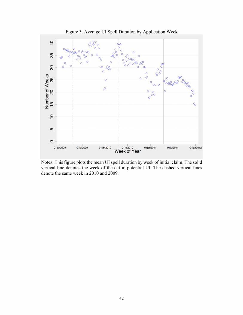
42

Figure 3. Average UI Spell Duration by Application Week

Notes: This figure plots the mean UI spell duration by week of initial claim. The solid vertical line denotes the week of the cut in potential UI. The dashed vertical lines denote the same week in 2010 and 2009.

43

Figure 4. Probability UI Spell Duration Exceeds Threshold 20 Weeks

40 Weeks

55 Weeks

60 Weeks

Notes: The figures plot the probability that UI spell durations exceed 20, 40, 55, and 60 weeks, by initial claim week. The solid vertical lines denote the week of the UI potential duration cut. The dashed vertical lines represent the same week in 2010.

44

Figure 5. RDD Estimates of the Differential Probability of Claiming UI for Weeks 1-73 of the Spell, Treatment - Control

Notes: Each point is an RDD estimate (local linear regression with IK optimal bandwidth with triangular kernel) for the probability that a recipient claims X weeks of UI, for X spanning 1 to 73. The dashed lines are the 95 percent confidence interval.

Figure 6. Treatment and Control Survivor and Hazards Functions at the Policy Threshold Panel A: Survivor Functions

Panel C: Hazard rates (-1*Derivative of Log Survivor Fct.)

Panel B: Log of the Survivor Functions

Panel D: Difference in the hazard rates

46

Notes: Panel A plots the RDD estimate of the survivor function. Each point in the control series is the estimated intercept for the control group in the local linear regression used to estimate the RDD probabilities of survival up to a given week, shown in in Figure 6. Each point in the treatment is the corresponding estimate for the treatment. The difference in these two series are the RDD estimates shown in Figure 6. Panel B plots the natural log of the survivor functions. Panel C plots -1 times the numerical derivative of the smoothed survivor functions. To smooth the survivor functions, we estimate a local quadratic regression with a bandwidth of 4 separately for the 1–20 week and the 21–57 week segments for the treatment group and the 1-26 week and 26-73 week segments for the control group. The segments are split this way to avoid the discontinuous drop in enrollment from recipients not enrolling into the EUC program. Panel D shows the difference in the estimated hazards in Panel C.

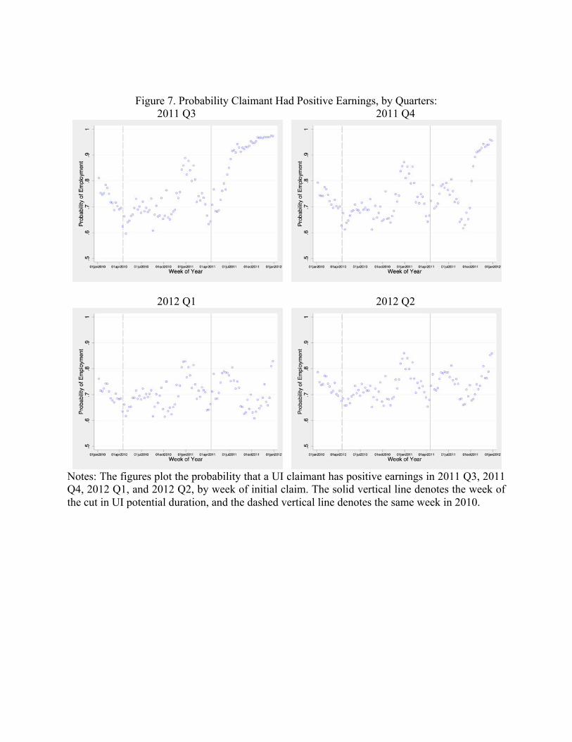
Figure 7. Probability Claimant Had Positive Earnings, by Quarters: 2011 Q3

2011 Q4

2012 Q1

2012 Q2

Notes: The figures plot the probability that a UI claimant has positive earnings in 2011 Q3, 2011 Q4, 2012 Q1, and 2012 Q2, by week of initial claim. The solid vertical line denotes the week of the cut in UI potential duration, and the dashed vertical line denotes the same week in 2010.

48

Figure 8. RDD Estimates of the Probability of Positive Earnings by Quarter following April 2011 UI Duration Cut

Notes: Each point is the RDD estimate (local linear regression with IK optimal bandwidth with triangular kernel) for the probability that a UI claimant has positive earnings in each quarter after the cut in potential UI duration. The dashed lines are the 95 percent confidence interval.

49

Figure 9. Log Reemployment Wage

Notes: The figure plots the mean of log earnings for the first complete quarter of earnings after a UI claim.

50

Figure 10. Placebo Distribution

Notes: This figure shows the distribution of placebo RDD estimates for unemployment insurance spell durations, where we vary the placebo treatment date over all weeks from January-October for years 2003-2012. Vertical line indicates the real treatment.

51

Figure 11. RDD Estimates of the Probability of Positive Earnings by Quarter After April 2010 Placebo Cut

Notes: Each point is the RDD estimate (local linear regression with IK optimal bandwidth with triangular kernel) for the probability that a UI claimant has positive earnings setting the UI benefit cut threshold to April 2010, one year prior to the actual cut in UI duration. The dashed line is the 95 percent confidence interval.

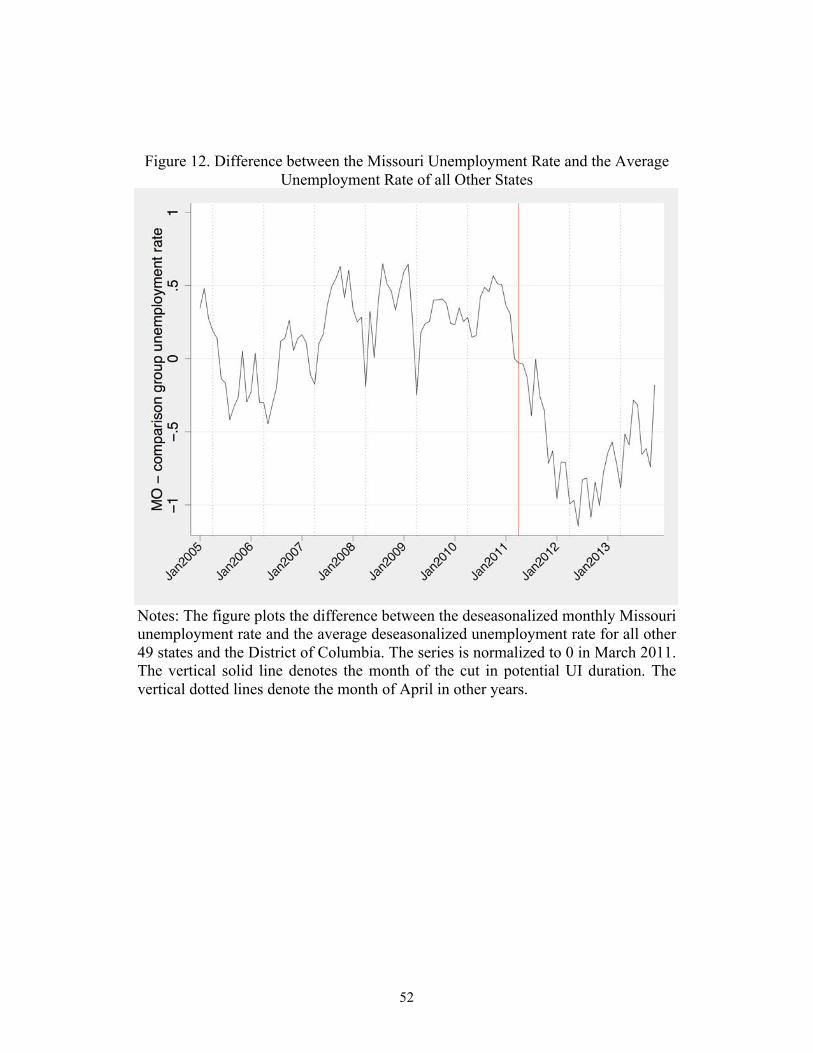
52

Figure 12. Difference between the Missouri Unemployment Rate and the Average Unemployment Rate of all Other States

Notes: The figure plots the difference between the deseasonalized monthly Missouri unemployment rate and the average deseasonalized unemployment rate for all other 49 states and the District of Columbia. The series is normalized to 0 in March 2011. The vertical solid line denotes the month of the cut in potential UI duration. The vertical dotted lines denote the month of April in other years.

53

Figure 13. Difference Between the Missouri Unemployment Rate and the Synthetic Control Unemployment Rate

Notes: The figure plots the difference between the monthly deseasonalized Missouri unemployment rate and the deseasonalized unemployment rate of the synthetic control. See text for details on the construction of the synthetic control. The vertical solid line denotes the month of the cut in potential UI duration. The vertical dotted lines denote the month of April in other years.

54

Figure 14. Difference Between the Missouri Unemployment Rate and Neighboring States

Unemployment Rate

Notes: The figure plots the difference between the deseasonalized monthly Missouri unemployment rate and the average deseasonalized unemployment rate for neighboring states. The series is normalized to 0 in March 2011. The vertical solid line denotes the month of the cut in potential UI duration. The vertical dotted lines denote the month of April in other years.

55

Figure 15. Predicted Change in the Missouri Unemployment Rate versus Difference-in-Difference Estimates of the Change in the Actual Missouri Unemployment Rate

Notes: The “Predicted Change” is the change in the Missouri unemployment rate that is predicted by the estimated RDD change in the survivor function assuming no spillover effects. “Actual – All states” is the difference between the Missouri unemployment rate and the unweighted average of the unemployment rate in all other states relative to March 2011. “Actual – Synthetic” is the difference between the Missouri unemployment rate and the synthetic control unemployment rate. “Actual – Neighbor states” is the difference between the Missouri unemployment rate and the unemployment rate of neighboring states. See text for details on the construction of the synthetic control.

56

Table 1. Summary Statistics 2003-2013 2011 Weekly benefit 260.4 259.6 [65.62] [74.19] Maximum benefit 6321 6328 [1976] [2727] Total benefits 3563 4234 [2769] [3429] Reemployment quarterly wage 7720 7240 [6901] [5703] Previous employer quarterly 9021 8259 wage [8072] [6891] Previous employment tenure 12.1 14.5 [9.50] [11.18] Jobless quarters 1.9 1.7 [5.23] [3.02] Weeks received 22.0 29.3 [18.92] [23.22] Notes: Standard deviations in brackets. Maximum benefit is the maximum dollars of regular state benefits available to the UI recipient. Total benefit is the total amount of UI benefits received in the spell. Weekly, maximum and total benefits pertain only to regular UI benefits and not EUC and EB. Reemployment quarterly wage is earnings for the first complete quarter of employment after the UI claim. Previous employer quarterly wage is earnings for the last complete quarter of employment before the unemployment claim. Previous employment tenure is in quarters. Weeks received refers to both regular and extended benefits.

57

Table 2. RDD Diagnostics

Claim

Frequency Log Predicted Duration Index

(1) (2) Estimated Discontinuity 3.13 -0.025 (824.2) (0.045) Observations 525 525 Bandwidth 9.64 3.91 Mean of Dependent Variable 5396.76 2.56 Notes: Local quadratic (column 1) and local linear (column 2) RDD estimates with a triangular kernel. Observations are at the claim week level. Models are estimated using weekly averages of the dependent variable, weighting observations by the number of observations in the cell. Column (1) reports the RDD estimate for the number of full eligibility initial UI claims. Column (2) reports the RDD estimate for the index of predicted log initial UI duration which is constructed by regressing log UI duration on a fourth-order polynomial of earnings in the quarter preceding job loss, indicators for four-digit industry, and previous job tenure quintiles.

58

Table 3. RDD Estimates of the Effect of the Cut in UI Potential Duration on Weeks of UI Received

Weeks Received

(1)

Received at least 20 Weeks

(2)

Received at least 40 Weeks

(3)

Received at least 55 Weeks

(4)

Received at least 60 Weeks

(5) Estimated Discontinuity -7.19 -0.075 -0.091 -0.079 -0.235 (0.818) (0.013) (0.011) (0.014) (0.013) Observations 524 524 524 524 524 Bandwidth 15.31 6.18 5.58 5.20 4.89 Mean of Dependent Variable 25.52 0.46 0.25 0.16 0.11 Notes: Local linear RDD estimates using the IK optimal bandwidth and a triangular kernel. Observations are at the claim week level. Models are estimated using weekly averages of the dependent variable, weighting observations by the number of observations in the cell. Placebo estimates are from estimating the same specification with a threshold set to one year prior to the April 2011 cut in benefits duration.

59

Table 4. RDD Estimates of the Effect of the Cut in UI Maximum Duration on Employment and Reemployment Wages

Pr(Earnings>0 in Q=0) (1)

Pr(Earnings>0 in Q=1) (2)

Pr(Earnings>0 in Q=2) (3)

Pr(Earnings>0 in Q=3) (4)

First complete quarter log reemployment

wage (5)

Estimated Discontinuity -0.029 0.085 0.082 0.072 0.035 (0.010) (0.020) (0.024) (0.022) (0.037) Observations 103 103 103 103 524 Bandwidth 5.21 6.08 5.97 5.78 7.38 Mean of Dependent Variable 0.84 0.80 0.75 0.71 8.60 Notes: Local linear RDD estimates using the IK optimal bandwidth and a triangular kernel. Observations are at the claim week level. Models are estimated using weekly averages of the dependent variable, weighting observations by the number of observations in the cell. Q=0 is 2011 Q2 for the main estimates and 2010 Q2 for the placebo estimates. Placebo estimates are from estimating the same specification with a threshold of one year prior to the April 2011 cut in benefits duration.

60

Table 5. DiD Estimates of the Change in the Missouri Unemployment Rate, Log Number of Unemployed, and Log Size of the Labor Force following the April 2011 UI Maximum Duration Cut

UR (1)

UR (2)

UR (3)

ln(U) (4)

ln(U) (5)

ln(U) (6)

LFP (7)

LFP (8)

LFP (9)

Panel A. All States Missouri * Post -0.89 -0.80 -0.85 -0.12 -0.10 -0.10 -0.07 -0.47 0.076 SE (0.12) (0.25) (0.02) (0.03) (0.16) (0.31) PCSE (0.19) (0.21) (0.02) (0.03) (0.26) (0.31) Wild Bootstrap C.I. (-1.1, -0.6) (-0.9, -0.7) (-0.15, -0.09) (-0.12, -0.08) (-0.3, 0.2) (-0.7, -0.3) %-tile rank 0.059 0.020 0.039 0.078 0.020 0.039 0.255 0.353 0.157 Observations 2856 2856 2576 2856 2856 2576 2856 2856 2576 Panel B. Neighbors Missouri * Post -1.0 -0.75 -0.70 -0.11 -0.08 -0.11 0.03 -0.42 -0.46 SE (0.11) (0.22) (0.01) (0.03) (0.16) (0.32) PCSE (0.20) (0.19) (0.03) (0.03) (0.30) (0.26) Wild Bootstrap C.I. (-1.3, -0.7) (-0.9, -0.6) (-0.14, -0.08) (-0.11, -0.06) (-0.44, 0.48) (-0.79, -0.14) %-tile rank 0.000 0.000 0.000 0.000 0.000 0.000 0.333 0.111 0.111 Observations 504 504 448 504 504 448 504 504 448 Predicted change -0.48 -0.48 -0.48 -0.07 -0.07 -0.07 Pred. chg. w/ outlier -0.64 -0.64 -0.64 -0.10 -0.10 -0.10 MO*trend X X X Synthetic control X X X

61

Notes: Observations are state by month units. UR is the unemployment rate, ln(U) is the natural log of the number of unemployed, and LFP is labor force participation as a percent of the civilian noninstitutional population. Variables are derived from the BLS Local Area Unemployment Statistics and deseasonalized as described in the text. All models in Panel A include the interaction of year×month and the percent of employment in agriculture, mining, utilities and construction, the percent of employment in manufacturing, the percent of employment in retail and wholesale trade, the percent change in housing values from 1999–2006, the percent change in housing values from 2007–2010, and the percent of the state population that is living in rural areas. The sample spans January 2009 to August 2013. SE is the OLS standard error, PCSE is the panel corrected standard error, and the permutation %-tile rank is the percentage of states that have a more negative “effect” when estimating the same model assigning each state to be the “treated” state in each permutation. MO*trend allows for a Missouri specific trend. The synthetic control uses weights from the synthetic control method described in the text to form a control group. Predicted change is the change in UR and ln(U) that is predicted by the RDD estimates of the change in the survivor function assuming no spillover effects. “Pred. chg. w/ outlier” is the same prediction with the outlier cohort.

62

Table 6. Ibragimov and Müller p-values by Block Sizes

(1)

56 blocks (2)

28 blocks (3)

14 blocks (4)

8 blocks (5)

6 blocks (6)

4 blocks Panel A. Unweighted Control; All States (Estimate = -0.95) t-statistic 13.50 9.94 7.95 6.62 6.34 14.26 Two-tail p-value (N-2 DOF) 0.00 0.00 0.00 0.01 0.02 0.04 N 56 28 14 8 6 4 Panel B. Synthetic Control; All States (Estimate = -0.86) t-statistic 12.20 9.13 6.98 5.74 5.19 4.58 Two-tail p-value (N-2 DOF) 0.00 0.00 0.00 0.01 0.04 0.14 N 56 28 14 8 6 4 Panel C. Unweighted Control; Neighbors (Estimate = -1.01) t-statistic 12.01 8.72 6.53 5.15 4.54 3.75 Two-tail p-value (N-2 DOF) 0.00 0.00 0.00 0.00 0.02 0.09 N 56 28 14 8 6 4 Panel D. Synthetic Control; Neighbors (Estimate = -0.73) t-statistic 8.68 6.38 4.85 3.82 3.30 2.34 Two-tail p-value (N-2 DOF) 0.00 0.00 0.00 0.01 0.03 0.15 N 56 28 14 8 6 4

Notes: Each column reports the t-statistic and corresponding two-tail p-value with N-2 degrees of freedom for the two-sample t-test of equality of the difference between the Missouri and comparison group unemployment rate before and after the potential duration cut, where the monthly Missouri – comparison group unemployment rate differences have been collapsed into the specified number of blocks. In Panel A the comparison group is the equally weighted average of the monthly unemployment rate for all states and the District of Columbia excluding Missouri. In Panel B, the comparison group is the synthetic control discussed in the text. We limit the sample to 28 months on each side of the policy change. Unemployment rates are derived from BLS LAUS. See Appendix Table 10 for the same tests using BLS CPS data.

63

Table 7. Comparison of Bordering Counties

UR (1)

UR (2)

ln(U) (3)

ln(U) (4)

ln(LF) (5)

ln(LF) (6)

Missouri * Post -0.77 -0.88 -0.08 -0.09 0.003 0.000 SE (0.08) (0.13) (0.01) (0.01) (0.023) (0.035) County Cluster SE (0.17) (0.09) (0.02) (0.01) (0.007) (0.002) Observations 4620 4620 4620 4620 4620 4620 State F.E. X X X X X X Time F.E. X X X X X X County-Pair FE X X X X X X MO*trend X X X Notes: This table uses LAUS unemployment data from 2009 through 2013 where an observation is the unemployment rate in a county-month. We match each treatment county on Missouri’s border to a neighboring untreated county in the adjoining state which we call county pairs. UR is the unemployment rate, ln(U) is the natural log of the number of unemployed, and ln(LF) is the natural log of the size of the labor force. MO*trend allows for a Missouri specific trend.

64

Online Appendix

Appendix Figure 1. Local Quadratic Fit in the Frequency Distribution of Full Eligibility Claims Underlying Column 1 of Table 2.

65

Appendix Figure 2. RDD Estimate of Total Weeks Received by Bandwidth (multiple of the IK

bandwidth)

Notes: Each point represents the local linear RDD estimate with bandwidth as a multiple of the IK bandwidth, along with the 95 percent confidence interval.

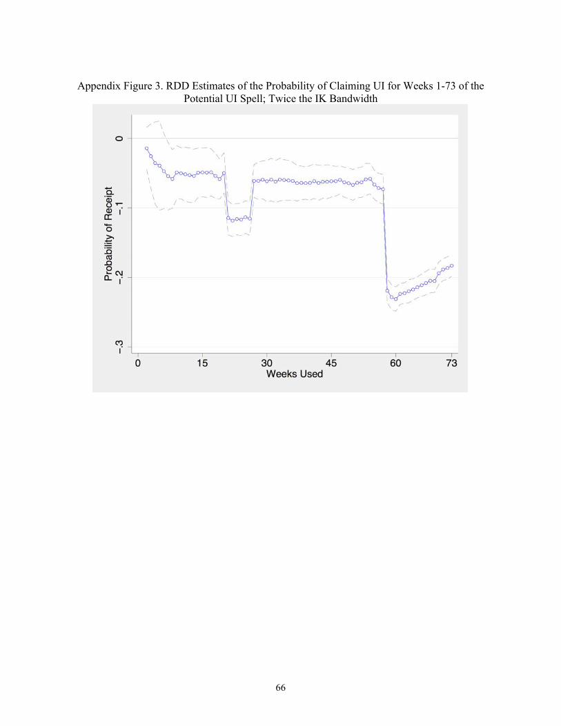
66

Appendix Figure 3. RDD Estimates of the Probability of Claiming UI for Weeks 1-73 of the

Potential UI Spell; Twice the IK Bandwidth

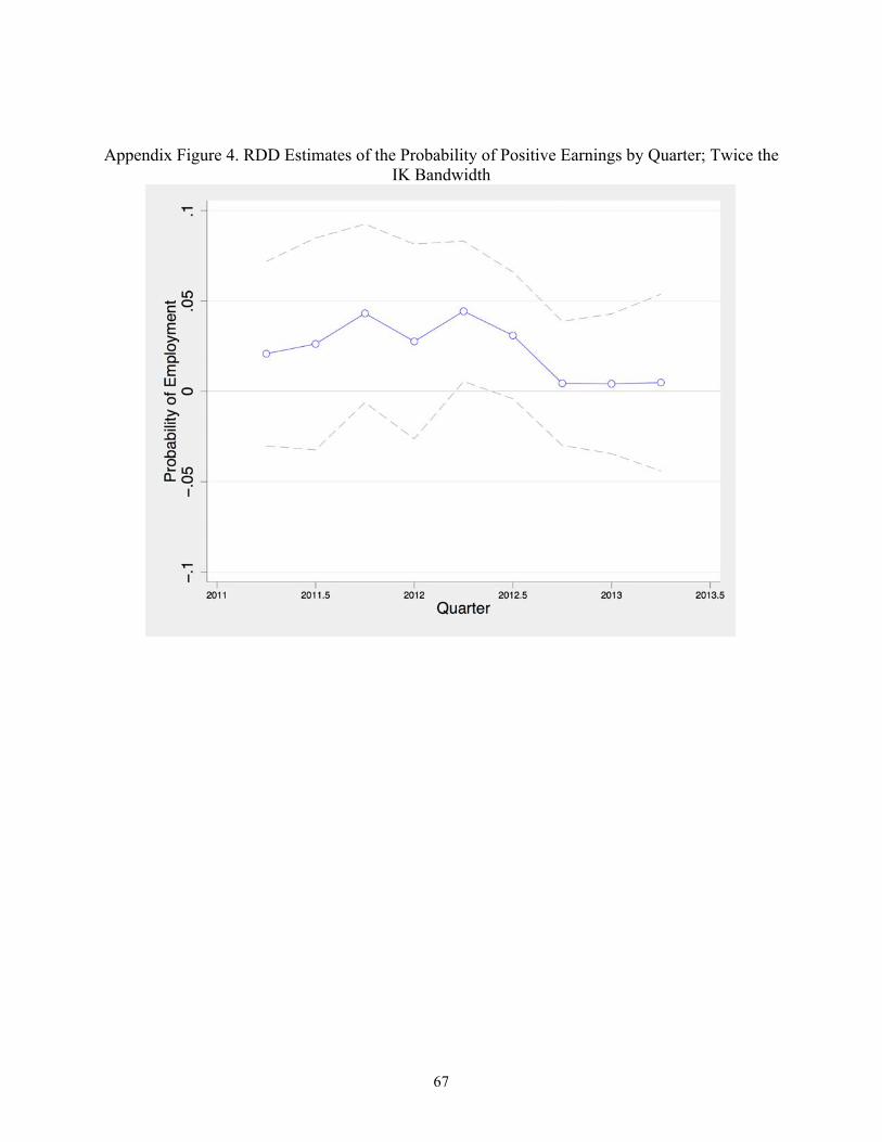
67

Appendix Figure 4. RDD Estimates of the Probability of Positive Earnings by Quarter; Twice the IK Bandwidth

68

Appendix Figure 5. Distribution of placebo estimates for unemployment insurance duration and employment for the March 2011–October 2011 period of placebo dates

Panel A. Unemployment insurance duration

Panel B. Probability employed in 2011Q3

Panel C. Probability employed in 2011Q4

Panel D. Probability employed in 2012Q1

Notes: This figure shows the placebo distribution of estimates for three outcomes where we vary the placebo treatments for each week, starting one month prior to the real policy change through six months after the policy change. All estimates use an IK bandwidth. The purpose of the figure is to show placebo estimates for a period when the labor market in Missouri was improving. The RDD estimate for the real policy change is denoted by the vertical line.

69

Appendix Figure 6. Unemployment rate in Missouri and other states; LAUS Panel A: All states

Panel C: Neighboring states

Panel B: All states, weighted

Panel D: Neighboring states, weighted

Notes: Data are seasonally unadjusted. Weights are the synthetic weights described in the text. Vertical bar is the month of the policy change.

46

810

Unem

ploy

men

t rat

e

2004m1 2006m1 2008m1 2010m1 2012m1 2014m1date

Missouri Other states

46

810

Unem

ploy

men

t rat

e

2004m1 2006m1 2008m1 2010m1 2012m1 2014m1date

Missouri Other states

46

810

Unem

ploy

men

t rat

e

2004m1 2006m1 2008m1 2010m1 2012m1 2014m1date

Missouri Other states

46

810

12Un

empl

oym

ent r

ate

2004m1 2006m1 2008m1 2010m1 2012m1 2014m1date

Missouri Other states

70

Appendix Figure 7. Unemployment rate in Missouri and other states; CPS Panel A: All states

Panel C: Neighboring states

Panel B: All states, weighted

Panel D: Neighboring states, weighted

Notes: Data are seasonally unadjusted. Weights are the synthetic weights described in the text. Vertical bar is the month of the policy change.

46

810

12Un

empl

oym

ent r

ate

2004m1 2006m1 2008m1 2010m1 2012m1 2014m1date

Missouri Other states

46

810

12Un

empl

oym

ent r

ate

2004m1 2006m1 2008m1 2010m1 2012m1 2014m1date

Missouri Other states

46

810

12Un

empl

oym

ent r

ate

2004m1 2006m1 2008m1 2010m1 2012m1 2014m1date

Missouri Other states

46

810

12Un

empl

oym

ent r

ate

2004m1 2006m1 2008m1 2010m1 2012m1 2014m1date

Missouri Other states

71

Appendix Figure 8. Difference Between the Missouri Unemployment Rate and the Neighbors-

Derived Synthetic Control Unemployment Rate

Notes: The figure plots the difference between the monthly deseasonalized Missouri unemployment rate and the deseasonalized unemployment rate of the synthetic control derived from neighboring states. The donor pool excludes Arkansas because it changed UI benefit duration over the same period. See text for details on the construction of the synthetic control. The control group consists of the following weighted average of states: 38.7 percent Illinois, 5.6 percent Nebraska, and 55.7 percent Kentucky. The vertical solid line denotes the month of the cut in potential UI duration. The vertical dotted lines denote the month of April in other years.

-1-.5

0.5

1M

O -

synt

hetic

con

trol u

nem

ploy

men

t rat

e

Jan2009 Jan2010 Jan2011 Jan2012 Jan2013

72

Appendix Figure 9. Predicted Change in the Missouri Unemployment Rate versus Difference-in-Difference Estimates of the Change in the Actual Missouri Unemployment Rate; Including

Outlier Cohort

Notes: The “Predicted Change” is the change in the Missouri unemployment rate that is predicted by the estimated RDD change in the survivor function assuming no spillover effects. “Actual – All states” is the difference between the Missouri unemployment rate and the unweighted average of the unemployment rate in all other states relative to March 2011. “Actual – Synthetic” is the difference between the Missouri unemployment rate and the synthetic control unemployment rate. “Actual – Neighbor states” is the difference between the Missouri unemployment rate and the unemployment rate of neighboring states. See text for details on the construction of the synthetic control. Predicted change is from micro estimates that include the outlier cohort.

-1.5

-1-.5

0.5

Cha

nge

in th

e un

empl

oym

ent r

ate

May2011 Nov2011 May2012 Nov2012 May2013

Predicted Change Actual - All statesActual - Synthetic Actual - Neighbor states

73

Appendix Figure 10. Employment-to-Population Ratio in Missouri relative to other States

Panel A. Comparison group is all other states

Panel B. Synthetic control

Panel C. Comparison group is neighboring states

-.015

-.01

-.005

0.0

05.0

1M

O -

com

paris

on g

roup

une

mpl

oym

ent r

ate

Jan2

005

Jan2

006

Jan2

007

Jan2

008

Jan2

009

Jan2

010

Jan2

011

Jan2

012

Jan2

013

-.01

-.005

0.0

05.0

1M

O -

synt

hetic

con

trol u

nem

ploy

men

t rat

e

Jan2009 Jul2010 Jan2012 Jul2013

-.01

0.0

1.0

2M

O -

com

paris

on g

roup

une

mpl

oym

ent r

ate

Jan2

005

Jan2

006

Jan2

007

Jan2

008

Jan2

009

Jan2

010

Jan2

011

Jan2

012

Jan2

013

74

Appendix Figure 11. Example of a Missouri Division of Employment Security Notice of Initial Determination of UI Status

75

Appendix Table 1. RDD Estimates of the Effect of the Cut in UI Potential Duration on Weeks of UI Received; Local Linear with IK Bandwidth Including Outlier Cohort

Weeks Received

(1)

Received at least 20 Weeks

(2)

Received at least 40 Weeks

(3)

Received at least 55 Weeks

(4)

Received at least 60 Weeks

(5) Estimated Discontinuity -8.697 -0.123 -0.118 -0.101 -0.236 (1.424) (0.057) (0.035) (0.035) (0.013) Observations 525 525 525 525 525 Bandwidth 14.94 6.15 6.08 5.17 4.92 Mean of Dependent Variable 25.45 0.46 0.25 0.16 0.11 Notes: Local linear RDD estimates using the IK optimal bandwidth and a triangular kernel. Observations are at the claim week level. Models are estimated using weekly averages of the dependent variable, weighting observations by the number of observations in the cell.

Appendix Table 2. RDD Estimates of the Effect of the Cut in UI Potential Duration on Weeks of UI Received; Local Quadratic with CCT Bandwidth

Weeks Received

(1)

Received at least 20 Weeks

(2)

Received at least 40 Weeks

(3)

Received at least 55 Weeks

(4)

Received at least 60 Weeks

(5) Estimated Discontinuity -9.511 -0.140 -0.115 -0.090 -0.247 (1.331) (0.031) (0.019) (0.016) (0.011) Observations 524 524 524 524 524 Bandwidth 25.00 23.04 25.65 22.25 29.93 Mean of Dependent Variable 25.45 0.46 0.25 0.16 0.11 Notes: Local quadratic RDD estimates using the CCT optimal bandwidth and a triangular kernel. Observations are at the claim week level. Models are estimated using weekly averages of the dependent variable, weighting observations by the number of observations in the cell.

76

Appendix Table 3. Estimated Effects at Placebo Discontinuities

Estimate SE N (1) (2) (3) 2012 -0.373 (1.804) 525 2011 -7.185 (0.818) 524 2010 -0.602 (0.611) 525 2009 -0.846 (0.532) 525 2008 -1.485 (0.866) 525 2007 1.977 (2.167) 525 2006 1.902 (1.651) 525 2005 -0.514 (1.275) 525 2004 2.279 (2.362) 525 2003 -0.265 (0.232) 525 Notes: This table presents the specification in column (1) of Table 3 for the treatment week in all available years. The year of the actual policy change is 2011.

Appendix Table 4. Estimating Column (1) of Table 3 with Deseasonalizing Data (1) (2) (3) (4) Estimated Discontinuity -8.548 -7.314 -8.705 -8.584 (1.267) (0.664) (1.834) (1.439) Observations 51 51 51 51 Bandwidth 13.09 12.16 11.74 14.13 Mean of Dependent Variable (2010) 33.15 33.15 33.15 33.15

Recession Era Control X All Years Control X 2010 Control X 2012 Control X Notes: To deseasonalize UI spell duration we regress this variable on week-specific fixed effects in non-treatment years and subtract out the resulting seasonal effects in the treatment-year data. We present several estimates using alternative years to estimate seasonality (Recession Era Control includes 2008-2011, All Years Control estimates the seasonal variation using all years other than the treatment year, 2010).

77

Appendix Table 5. Excluding Seasonal Industries

Omit Seasonal

Industries (1)

Omit Manufacturing (2)

Panel A. Main Estimates Estimated Discontinuity -6.713 -7.960 (1.424) (1.738)

Observations 9253 10709 Bandwidth 14.1 13.3 Mean of Dependent Variable 29.9 29.3 Panel B. Placebo Estimates Estimated Discontinuity 0.207 -0.215 (1.381) (2.558) Observations 8720 10177 Bandwidth 13.7 11.0 Mean of Dependent Variable 35.5 34.9 Notes: We test whether the estimates we obtained in column (1) of Table 3 are robust to the exclusion of the more seasonal industries. To this end, we first estimate seasonality by regressing claim quantities on month dummies and calculating the variance in the month dummies for each two-digit NAICS industry. We then re-estimate our main effect while excluding the most seasonal 25 percent of industries (column 1). We also test whether the estimate is robust to excluding manufacturing claims (column 2).

78

Appendix Table 6. Utah Placebo Weeks Received

(1)

Panel A. Main Estimates

Estimated Discontinuity -0.227 (0.327) Observations 359 Bandwidth 12.26 Mean of Dependent Variable 10.43 Panel B. Placebo Estimates Estimated Discontinuity 0.494 (0.300) Observations 359 Bandwidth 11.72 Mean of Dependent Variable 11.67 Notes: As a placebo, we use administrative data from the state of Utah to estimate the same RD as in Missouri in a state where UI parameters were unchanged. The structure of the data and specification is identical to column (1) of Table 3.

79

Appendix Table 7. RDD Estimates of the Effect of the Cut in UI Maximum Duration on Employment and Reemployment Wages; Local Linear with IK Bandwidth and Including Outlier Cohort

Employed 2011Q2

(1)

Employed 2011Q3

(2)

Employed 2011Q4

(3)

Employed 2012Q1

(4)

First complete quarter log reemployment wage

(5) Estimated Discontinuity -0.022 0.119 0.112 0.106 0.121 (0.014) (0.039) (0.041) (0.044) (0.118) Observations 104 104 104 104 525 Bandwidth 5.21 6.08 5.97 5.78 7.38 Mean of Dependent Variable 0.84 0.80 0.75 0.71 8.60 Notes: Local linear RDD estimates using the IK optimal bandwidth and a triangular kernel. Observations are at the claim week level. Models are estimated using weekly averages of the dependent variable, weighting observations by the number of observations in the cell. Placebo estimates are from estimating the same specification with a threshold of one year prior to the April 2011 cut in benefits duration.

Appendix Table 8. RDD Estimates of the Effect of the Cut in UI Maximum Duration on Employment and Reemployment Wages; Local Polynomial with CCT Bandwidth

Employed 2011Q2

(1)

Employed 2011Q3

(2)

Employed 2011Q4

(3)

Employed 2012Q1

(4)

First complete quarter log reemployment wage

(5) Estimated Discontinuity -0.022 0.094 0.095 0.060 0.203 (0.016) (0.037) (0.040) (0.038) (0.112) Observations 103 103 103 103 524 Bandwidth 13.49 11.2 10.53 11.11 16.61 Mean of Dependent Variable 0.84 0.80 0.75 0.71 8.60 Notes: Local quadratic RDD estimates using the CCT bandwidth and a triangular kernel. Observations are at the claim week level. Models are estimated using weekly averages of the dependent variable, weighting observations by the number of observations in the cell. Placebo estimates are from estimating the same specification with a threshold of one year prior to the April 2011 cut in benefits duration.

80

Appendix Table 9. DiD Estimates of the Change in the Missouri Unemployment Rate, Log Number of Unemployed, and Log Size of the Labor Force following the April 2011 UI Maximum Duration Cut; Current Population Survey Sample

UR (1)

UR (2)

UR (3)

ln(U) (4)

ln(U) (5)

ln(U) (6)

LFP (7)

LFP (8)

LFP (9)

Panel A. All States Missouri * Post -0.805 -0.826 -1.07 -0.111 -0.117 -0.14 -0.41 -0.76 -0.325 SE (0.279) (0.558) (0.039) (0.079) (0.41) (0.82) PCSE (0.897) (1.24) (0.031) (0.086) (0.50) (1.05) Wild Bootstrap C.I. (-1.1, -0.5) (-1.0, -0.6) (-0.14, -0.08) (-0.15, -0.09) (-0.74, -0.03) (-1.19, -0.42) %-tile rank 0.078 0.098 0.059 0.118 0.039 0.078 0.353 0.196 0.255 Observations 2856 2856 2576 2856 2856 2576 2856 2856 2576 Panel B. Neighbors Missouri * Post -0.900 -0.656 -0.745 -0.107 -0.078 -0.125 -0.42 -0.72 -0.86 SE (0.263) (0.526) (0.038) (0.077) (0.43) (0.86) PCSE (0.332) (0.425) (0.038) (0.058) (0.60) (1.08) Wild Bootstrap C.I. (-1.3, -0.5) (-0.9, -0.4) (-0.15, -0.05) (-0.12, -0.04) (-1.1, 0.1) (-1.2, -0.3) %-tile rank 0.111 0.111 0.000 0.000 0.111 0.000 0.333 0.222 0.111 Observations 504 504 448 504 504 448 504 504 448 Predicted change -0.48 -0.48 -0.48 -0.07 -0.07 -0.07 Pred chg. w/ outlier -0.64 -0.64 -0.64 -0.10 -0.10 -0.10 MO*trend X X X Synthetic control X X X

81

Notes: Observations are state by month units. UR is the unemployment rate, ln(U) is the natural log of the number of unemployed, and LFP is labor force participation as a percent of the civilian noninstitutional population. Variables are derived from the BLS Current Population Survey and deseasonalized as described in the text. All models in Panel A include the interaction of year×month and the percent of employment in agriculture, mining, utilities and construction, the percent of employment in manufacturing, the percent of employment in retail and wholesale trade, the percent change in housing values from 1999–2006, the percent change in housing values from 2007–2010, and the percent of the state population that is living in rural areas. The sample spans January 2009 to August 2013. SE is the OLS standard error, PCSE is the panel corrected standard error, and the permutation %-tile rank is the percentage of states that have a more negative “effect” when estimating the same model assigning each state to be the “treated” state in each permutation. MO*trend allows for a Missouri specific trend. The synthetic control uses weights from the synthetic control method described in the text to form a control group. Predicted change is the change in UR and ln(U) that is predicted by the RDD estimates of the change in the survivor function assuming no spillover effects. “Pred. chg. w/ outlier” is the same prediction with the outlier cohort.

82

Appendix Table 10. Ibragimov and Müller p-values by Block Sizes; Variables Derived from Current Population Survey

(1)

56 blocks (2)

28 blocks (3)

14 blocks (4)

8 blocks (5)

6 blocks (6)

4 blocks Panel A. Unweighted Control; All States (Estimate = -0.86) t-statistic 3.85 4.60 5.68 4.38 9.72 6.29 Two-tail p-value (N-2 DOF) 0.00 0.00 0.00 0.02 0.01 0.10 N 56 28 14 8 6 4 Panel B. Synthetic Control; All States (Estimate = -1.03) t-statistic 4.22 4.55 5.07 4.19 9.83 46.96 Two-tail p-value (N-2 DOF) 0.00 0.00 0.00 0.02 0.01 0.01 N 56 28 14 8 6 4 Panel C. Unweighted Control; Neighbors (Estimate = -0.900) t-statistic 4.05 4.75 5.34 6.79 7.02 9.53 Two-tail p-value (N-2 DOF) 0.00 0.00 0.00 0.01 0.02 0.07 N 56 28 14 8 6 4 Panel D. Synthetic Control; Neighbors (Estimate = -0.75) t-statistic 3.07 3.71 4.87 8.08 3.70 18.72 Two-tail p-value (N-2 DOF) 0.00 0.00 0.00 0.00 0.07 0.03 N 56 28 14 8 6 4

Notes: Each column reports the t-statistic and corresponding two-tail p-value with N-2 degrees of freedom for the two-sample t-test of equality of the difference between the Missouri and comparison group unemployment rate before and after the potential duration cut, where the monthly Missouri – comparison group unemployment rate differences have been collapsed into the specified number of blocks. In Panel A the comparison group is the equally weighted average of the monthly unemployment rate for all states and the District of Columbia excluding Missouri. In Panel B, the comparison group is the synthetic control discussed in the text. We limit the sample to 28 months on each side of the policy change. Unemployment rates are derived from BLS CPS data.

83

Appendix Table 11. Comparison of Characteristics of Missouri and All Other States

Full sample Full sample Unemployed

sample Unemployed sample

Missouri All other states Missouri All other

states (1) (2) (3) (4) High School 40.7 37.7 60.8 57.1 Degree or Lower [49.1] [48.4] [48.7] [49.4] Bachelor’s Degree+ 15.4 20.7 6.0 15.7 [36.1] [40.5] [23.8] [36.4] Married 40.7 40.3 37.9 38.8 [49.1] [49.1] [48.5] [48.7] Never Married 21.4 23.6 40.3 40.1 [41.0] [41.5] [49.0] [49.0] Working Age 51.8 51.9 69.7 75.5 [50.0] [50.0] [46.0] [43.0] Seniors 12.7 12.9 1.2 3.2 [33.3] [33.5] [10.9] [17.5] Makes <30k 44.3 23.6 45.6 38.3 [44.3] [42.5] [49.8] [48.6] Makes <50k 43.8 41.6 62 59.9 [49.6] [49.3] [48.5] [49.0] Makes <75k 48.4 59 77.8 76.9 [48.4] [49.2] [41.6] [42.2] Black 11.7 12.5 17.5 18.2 [32.1] [33.1] [38.0] [38.6] Hispanic 3.4 15.8 3.8 18.6 [18.1] [36.5] [19.0] [38.8] Non-White 20.3 15.2 21.1 25.2 [40.2] [35.9] [40.8] [43.4] NILF 49.5 49.5 0.0 0.0 [50.0] [50.0] [0.0] [0.0] Unemployed 5.6 4.8 100 100 [22.9] [21.3] [0.0] [0.0] Observations 2,369 133,109 130 6,088

Notes: Data from the March 2010 Current Population Survey, weighted by the CPS household weights. Columns (1) and (2) compare the demographics of all Missourians to Americans that do not live in Missouri. Columns (3) and (4) compare demographics of Missouri’s unemployed to unemployed Americans that do not live in Missouri. Unemployed is as a percentage of the population.