Wavelet‐based multiscale performance analysis: An … ARTICLE 10.1002/2013WR014650 Wavelet-based multiscale performance analysis: An approach to assess and improve hydrological models

RESEARCH ARTICLE10.1002/2013WR014650

Wavelet-based multiscale performance analysis: An approachto assess and improve hydrological modelsMaheswaran Rathinasamy1, Rakesh Khosa1, Jan Adamowski2, Sudheer ch1, Partheepan G3,Jatin Anand1, and Boini Narsimlu1

1Department of Civil Engineering, Indian Institute of Technology Delhi, New Delhi, Delhi, India, 2Department ofBioresource Engineering, McGill University, Ste Anne de Bellevue, Quebec, Canada, 3Department of Civil Engineering,Amity University, Noida, Uttar Pradesh, India

Abstract The temporal dynamics of hydrological processes are spread across different time scales and, assuch, the performance of hydrological models cannot be estimated reliably from global performance measuresthat assign a single number to the fit of a simulated time series to an observed reference series. Accordingly, it isimportant to analyze model performance at different time scales. Wavelets have been used extensively in thearea of hydrological modeling for multiscale analysis, and have been shown to be very reliable and useful inunderstanding dynamics across time scales and as these evolve in time. In this paper, a wavelet-based multiscaleperformance measure for hydrological models is proposed and tested (i.e., Multiscale Nash-Sutcliffe Criteria andMultiscale Normalized Root Mean Square Error). The main advantage of this method is that it provides a quanti-tative measure of model performance across different time scales. In the proposed approach, model andobserved time series are decomposed using the Discrete Wavelet Transform (known as the �a trous wavelettransform), and performance measures of the model are obtained at each time scale. The applicability of theproposed method was explored using various case studies––both real as well as synthetic. The synthetic casestudies included various kinds of errors (e.g., timing error, under and over prediction of high and low flows) inoutputs from a hydrologic model. The real time case studies investigated in this study included simulationresults of both the process-based Soil Water Assessment Tool (SWAT) model, as well as statistical models, namelythe Coupled Wavelet-Volterra (WVC), Artificial Neural Network (ANN), and Auto Regressive Moving Average(ARMA) methods. For the SWAT model, data from Wainganga and Sind Basin (India) were used, while for theWavelet Volterra, ANN and ARMA models, data from the Cauvery River Basin (India) and Fraser River (Canada)were used. The study also explored the effect of the choice of the wavelets in multiscale model evaluation. Itwas found that the proposed wavelet-based performance measures, namely the MNSC (Multiscale Nash-SutcliffeCriteria) and MNRMSE (Multiscale Normalized Root Mean Square Error), are a more reliable measure than tradi-tional performance measures such as the Nash-Sutcliffe Criteria (NSC), Root Mean Square Error (RMSE), and Nor-malized Root Mean Square Error (NRMSE). Further, the proposed methodology can be used to: i) comparedifferent hydrological models (both physical and statistical models), and ii) help in model calibration.

1. Introduction

Hydrological modeling is essential for many watershed planning and management activities that oftenrequire guidance on problems such as optimal scheduling of projects, optimal scheduling of water releases,flood forecasting, and drought analysis [Nourani et al., 2014; Maheswaran et al., 2013]. The accuracy of ahydrological model depends on how well the model simulations match with observations of correspondingsystem state variables. Based on the performance of the model during the calibration stage, decisions needto be made to accept or revise the model with certain preferences, based upon available information andprior knowledge. In addition, the quantitative description of error is often the basis of uncertainty estima-tion in which multiple model runs are described in terms of their fit with data in order to quantify the uncer-tainty associated with model predictions [Beven and Binley, 1992]. This is very important as differentrealizations of the same model (i.e., model runs with different parameter sets) may not be distinguishablewith the data available for model assessment [Lane 2007].

Devising strategies for estimating model performance measures has evoked intense debate amongsthydrologists and its resolution is indeed a major challenge. While, in general, model evaluation is usually

Key Points:� New wavelet-based performance

measure developed� New measure more useful than

traditional measures� New measure can help improve a

hydrological model

Correspondence to:J. Adamowski,[email protected]

Citation:Rathinasamy, M., R. Khosa,J. Adamowski, S. ch, G. Partheepan,J. Anand, and B. Narsimlu (2014),Wavelet-based multiscale performanceanalysis: An approach to assess andimprove hydrological models, WaterResour. Res., 50, 9721–9737,doi:10.1002/2013WR014650.

Received 26 AUG 2013

Accepted 15 NOV 2014

Accepted article online 19 NOV 2014

Published online 31 DEC 2014

RATHINASAMY ET AL. VC 2014. American Geophysical Union. All Rights Reserved. 9721

Water Resources Research

PUBLICATIONS

http://dx.doi.org/10.1002/2013WR014650

http://onlinelibrary.wiley.com/journal/10.1002/(ISSN)1944-7973/

http://publications.agu.org/

based on the match between derived model simulations and the corresponding observed data, Lane et al.[1994] point out that a more rigorous internal analysis of the model results is necessary since output predic-tions may be reasonable while ‘‘model’’ internal predictions are incorrect––the correct result for the wrongreasons. Given limitations from the point of view of data availability, most research is based on output pre-diction rather than an objective internal analysis. Also, the quantitative description of accuracy normallytakes the form of an objective function, and it is recognized that many of the problems connected withobjective functions may be linked to the embedded assumptions made about the underlying properties ofmodel errors [Lane, 2007]. And finally, in general these objective functions are global in nature and therebyvery rarely pick up either the localization of the error at particular points in time, or the associated scale orfrequency at which these errors occur. Model comparison methods on the basis of outputs from a modelinclude: (i) visual comparison of the models using graphs such as line plots, scatter plots, bias plots; (ii) spec-tral methods [Whittle, 1982; Priestley, 1981; Montanari and Toth, 2007]; (iii) state space embeddingapproaches [Moeckel and Murray, 1997; Keylock, 2012]; and (iv) time domain-based statistical performancemeasures such as Root Mean Square Error [Wilmott, 1982], Nash-Sutcliffe Criteria [Nash and Sutcliffe,1970;McCuen and Snyder, 1975], amongst others. It must be noted, however, that each of these aforementionedapproaches have characteristic advantages and disadvantages.

Model performance may first be evaluated by a visual comparison of the observed and simulated flowhydrographs but this remains subjectively dependent on the evaluator’s experience [Chiew et al., 1993;Houghton-Carr, 1999], besides being very cumbersome when many model runs are compared. Spectralmethods are robust in providing insight into model behavior in the frequency domain but are restricted bythe limitation that this is only applicable for stationary processes. Schaefli and Zehe [2009] comment thatmethods for hydrologic model comparison based on Fourier analysis might result in unreliable estimatesfor non Gaussian processes, or show an important loss of efficiency if the autocorrelation of the process ishigh. The state space embedding dimension approach is based on the Takens [1981] theorem of delayembedding. State space methods are advantageous compared to other methods in many ways, includingbeing a more sensitive measure of the dynamics of the system [Liu et al., 1998], and being more robust inmeasuring long term behavior [Moeckel and Murray, 1997]. However, all of these methods are restricted bythe following limitations: (a) the optimum embedded dimension has to be estimated a priori for modelcomparisons to be meaningful, (b) the approach does not work for higher dimensions and in the presenceof noise, (c) there is difficulty in creating artificial symmetry of the phase space as the embedding dimen-sion is increased, and (d) the methods may not work well for data which are intermittent, e.g., vonHardenberg et al. [1997] who showed that the standard algorithms fail to correctly estimate the dimensionsof processes characterized by intermittency while giving no warning of their failure.

Similarly, the time domain performance statistics such as Root Mean Square Error (RMSE), Correlation Coeffi-cient (CC), Nash-Sutcliffe Criterion (NSC), d (Index of Agreement), MAE (Mean Absolute Error) and NRMSE (Nor-malized Root Mean Square) have several limitations as pointed out by Schaefli and Gupta [2007]. Thesemeasures are dependent on the base reference model and do not measure how good a model is in an abso-lute sense. It is also stated that in the case of strongly seasonal time series, a model that only explains seasonal-ity but fails to reproduce any smaller time scale fluctuations will also report a satisfactory NSC value; whenpredictions are made at daily time steps, this (high) value will be misleading. In contrast, if the model isintended to simulate the fluctuations around a relatively constant mean value, the model can only obtain highNSC values if it explains the small time-scale fluctuations. Further, within the framework of NSC, timing errorsare heavily punished and, as a result, even reasonably satisfactory model results are given low NSC values.More generally, all the traditional performance measures are insufficient and only provide an overall perceptionabout the performance of the model by comparing two signals in the time and frequency domains separately.

In order to improve performance measures and obtain a better idea regarding hydrologic model perform-ance, attempts to modify traditional performance measures have been made. For example, Krause et al.[2005] evaluated different performance measures such as the NSE, modified NSE (using the logarithmicform of E and also a more generic form of NSE), R2, Index of agreement (d), and log modified R2, and alsoevaluated their ability to capture the underlying process, and showed that the modified versions of the per-formance measures were better for hydrological model assessment. There have been other attempts tomodify these measures; however, it is important to note that these measures still carry the restrictions ofstationarity besides being highly sensitive to some features of the time series.

Water Resources Research 10.1002/2013WR014650


In the past two decades, wavelet transforms have begun to be applied across a wide range of applica-tions [e.g., Adamowski et al., 2012; Campisi-Pinto et al., 2012; Nalley et al., 2013; Nourani et al., 2013;Adamowski and Prokoph, 2014; Belayneh et al., 2014]. Wavelets have also been applied in the area ofmodel performance analysis owing to their time frequency characterization and multi resolution capabil-ities. Lane [2007] used the continuous wavelet transform using the Gaussian wavelet to compare hydro-logical modeling results at different time scales from TOPMODEL. The results showed that the wavelet-based methodology was a promising approach. Schaefli and Zehe [2009] used the wavelet power spec-trum to compare simulated values with observed values of hydrological time series. The results showedthat the wavelet-based spectrum analysis of the observed and simulated values could easily pick up thesimilarities and dissimilarities across different time scales. In addition, calibration of the hydrologicalmodel was done in the wavelet domain rather than in the time domain using a wavelet-based metricderived from the Continuous Wavelet Transform (CWT). Jiang and Mahadevan [2011] used wavelet fea-tures such as the cross wavelet spectrum and wavelet coherence analysis for model validation ofmechanical dynamic systems. Even though Schaefli and Zehe’s [2009] work is very useful, it is based onthe metric derived from the difference between the observed and simulated series in the spectraldomain; in order to make the results more meaningful and easy to analyze, it was felt that further inves-tigations are required on the use of wavelet-based performance analysis in the time domain.

To the best knowledge of the authors, very little research has been done in the area of wavelet-based per-formance measures for hydrologic models. Therefore, the objectives of this paper are to:

1. Systematically evaluate the advantages of using wavelet-based performance measures over traditionalmeasures based on the time and frequency domain.

2. Develop a wavelet-based multiscale performance measure which reflects the ability of a hydrological modelto capture the underlying phenomena, and also provides a quantitative measure.

3. Use the proposed wavelet-based multiscale performance measure to identify the model parameters tobe altered and thereby attempt to improve model performance.

In the case studies presented (both the 9 synthetic case studies and the 4 real time case studies), resultsfrom the various models are compared with observations using traditional measures (NSC, NRMSE, MAE),and the two proposed wavelet-based performance measures: MNSC (Multiscale Nash-Sutcliffe Criteria) andMNRMSE (Multiscale Normalized Root Mean Square Error).

2. Wavelet Analysis

Wavelet analysis, initially formalized by Grossmann and Morlet [1984], results in a time frequency (or timescale) representation of a signal. Wavelet analysis transforms a signal into scaled and translated versions ofan original (mother) wavelet, instead of decomposing a signal into constituent harmonic functions as inFourier analysis. There are two types of wavelet transforms: the continuous wavelet transform (CWT), andthe discrete wavelet transform (DWT). CWT operates on smooth continuous functions and can detect anddecompose signals on all scales. DWT may use the Mallat or �a trous algorithms, which operate on scalesthat have discrete numbers. The scales and locations used in DWT are normally based on a dyadic arrange-ment (i.e., integer powers of two) [Nalley et al., 2012; Tiwari and Adamowski, 2013].

Although CWT is able to locate specific events in a signal that may not be obvious, one of the main disad-vantages of the CWT is that the construction of the CWT inverse is more complicated [Fugal, 2009]. In prac-tice this may not always be desirable because often, signal reconstructions are needed [Fugal, 2009]. It mayalso be more desirable to choose the DWT over CWT because CWT does not produce information in theform of a time series, but rather in a two-dimensional format [Percival, 2008].

2.1. Discrete Wavelet TransformThe DWT is an orthogonal function which can be applied to a finite group of data. Functionally, DWT hassimilar attributes to the Discrete Fourier Transform, namely: (i) the transforming function is orthogonal, (ii) asignal passed twice through the transformation is unchanged, (iii) the input signal is assumed to be a set ofdiscrete-time samples, and (iv) the transform operates as convolutions. However, while the basis function ofthe Fourier transform is a sinusoid, the wavelet basis, in contrast, is a set of functions which are defined by a



compactly supported, localized wavelet function. A typical discrete wavelet function can be represented as[Addison, 2010]

wj;kðtÞ52j2wð2j t2kÞ (1)

where w(t) is the mother wavelet function and j and k are the translation and dilation indices.

2.2. ‘‘�A trous’’ Wavelet Transform or MODWT (Maximal Overlap Discrete Wavelet Transform)In DWT, decimation is carried out so that only half of the coefficients of the detailed component are left atthe current level, and half of the coefficients of the smooth version are recursively processed using highpass and low pass filters for coarser resolution levels. Due to the decimation, the number of wavelet coeffi-cients is halved with each move to a coarser level. This problem may be overcome by introducing the sta-tionary Maximal Overlap Discrete Wavelet Transform (MODWT), alternatively known as the �a trous wavelettransform proposed by Shensa [1992]. The basic idea of the �a trous wavelet transform is to fill the resultinggaps using redundant information obtained from the original series. In this approach, the wavelet decom-position is derived by passing the given time series through a low pass filter and, as a result of this, the deri-vation of details and the smoothed version becomes possible. For example, consider the original time seriesx(t) which may also be denoted by co, or

c0ðtÞ5xðtÞ (2)

Further smoother versions of x(t) may be derived using

ciðtÞ5X1

l521hðlÞcj21ðt12i21lÞ (3)

In the preceding equation (3), i takes values from 1 to J (defined level of decomposition) and ‘‘h’’ is alow pass filter with compact support. The length and characteristics of the low pass filter will dependon the type of wavelet used. The simplest wavelet is the Haar wavelet with a low pass filter specifica-tion given by (1=2, 1=2). Similarly, the filter values for the B3 spline wavelet are defined as (1/16, 1/4, 3/8,1/4, 1/16).

Using the smoother versions of x(t) at level i and i-1, the detail component of x(t) at level i is defined as

diðtÞ5ci21ðtÞ2ciðtÞ (4)

The set {d1, d2. dp,cp} represents the additive wavelet decompositions of data up to a resolution level of pand the term cp in this set denotes the residual component, and is also termed as the approximation.Accordingly, for reconstruction, the inverse transform is given by

xðtÞ5cpðtÞ1Xp

i51

diðtÞ (5)

Here unlike the classical DWT, the decimation is avoided resulting in components at different time scales tobe of the same length. In this study, the WMTSA toolbox [Percival and Walden, 2000] was used for obtainingthe MODWT of the time series.

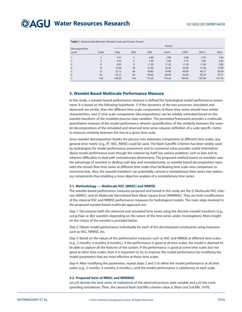
2.3. Wavelet Scale and Fourier Frequency (Period)In wavelet analysis, each of the scales carries a specific correspondence to the period (51/frequency). Therelationship between the period and scale is dependent on the wavelet function and the sampling period‘‘Dt.’’ Table 1 enumerates the scale and period relationship for some of the commonly used wavelets. ForHaar and Morlet functions, the two are nearly identical while for db2, the Fourier period is 1.5 times largerthan the scale. This ratio has no special significance and is due solely to the functional form of each waveletfunction [Torrence and Compo, 1998]. However, it is important to convert from scale to Fourier period beforeanalysing the results, as most probably one may be interested in understanding features of the signal at acertain scale in terms of the equivalent Fourier period. For example, if MODWT is applied for a monthly timeseries, the information at a time scale of D1 using the Haar wavelet corresponds to the features having aperiod of 2 months, whereas the same information obtained using db2 corresponds to a period of 3months. In this study, MATLAB function scal2freq has been used to find the relationship between scale andfrequency.



3. Wavelet-Based Multiscale Performance Measure

In this study, a wavelet-based performance measure is defined for hydrological model performance assess-ment. It is based on the following hypothesis: 1) if the dynamics of the two processes (simulated andobserved) are similar, then the different time scale components of these time series should have similarcharacteristics, and 2) time scale components (decompositions) can be reliably estimated based on thewavelet transform of the modeled process state variables. The presented framework provides a multiscalequantitative measure of the model performance wherein quantification of the similarity between the wave-let decompositions of the simulated and observed time series requires definition of a scale specific metricto measure similarity between the two at a given time scale.

Since wavelet decomposition breaks the process into stationary components at different time scales, anygeneral error metric (e.g., R2, NSC, RMSE) could be used. The Nash-Sutcliffe Criterion has been widely usedby hydrologists for model performance assessment and its numerical value provides useful informationabout model performance even though the criterion by itself has various problems such as bias and itsinherent difficulties to deal with nonstationary phenomena. The proposed method based on wavelets usesthe advantage of wavelets in dealing with bias and nonstationarity, as wavelet-based decomposition sepa-rates the stream flow time series at different time scales thus facilitating time scale wise comparison toovercome bias. Also, the wavelet transform can potentially convert a nonstationary time series into station-ary components thus enabling a more objective analysis of a nonstationary time series.

3.1. Methodology — Multiscale NSC (MNSC) and NRMSEThe wavelet-based performance measures proposed and tested in this study are the (i) Multiscale NSC crite-rion (MNSC), and (ii) Multiscale Normalized Root Mean Square Error (MNRMSE). They are both modificationsof the classical NSC and NRMSE performance measures for hydrological models. The main steps involved inthe proposed wavelet-based multiscale approach are:

Step 1: Decompose both the observed and simulated time series using the discrete wavelet transform (e.g.,using Haar or db2 wavelets depending on the nature of the time series under investigation). More insighton the choice of the wavelet is provided below.

Step 2: Obtain model performance individually for each of the decomposed constituents using measuressuch as NSC, NRMSE, etc.

Step 3: Based on the values of the performance measures such as NSC and NRMSE at different time scales(e.g., 2 months, 4 months, 8 months.), if the performance is good at all time scales, the model is deemed tobe able to capture all the features of the system. If the performance is good at some time scales but notgood at other time scales, then it is important to try to improve the model performance by modifying themodel parameters that are most effective at those time scales.

Step 4: After modifying the parameters, repeat steps 2 and 3 to refine the model performance at all timescales (e.g., 2 months, 4 months, 8 months.), until the model performance is satisfactory at each scale.

3.2. Proposed form of MNSC and MNRMSELet y(t) denote the time series of realizations of the observed process state variable and ys(t) the corre-sponding simulations. Then, the classical Nash-Sutcliffe criterion value is [Nash and Sutcliffe, 1970]

Table 1. Relationship Between Wavelet Scale and Fourier Period

DecompositionLevel Scale

Period

Haar Db2 Db4 Sym4 Coif4 Db10 Morl

1 2 2.01 3 2.80 2.80 2.88 2.92 2.462 4 4.02 6 5.60 5.60 5.75 5.85 4.923 8 8.03 12 11.20 11.20 11.50 11.69 9.854 16 16.06 24 22.40 22.40 23.00 23.38 19.695 32 32.13 48 44.80 44.80 46.00 46.77 39.386 64 64.25 96 89.60 89.60 92.00 93.54 78.777 128 128.50 192 179.20 179.20 184.00 187.08 157.54



NSC512

XN

t51

ysðtÞ2yðtÞ½ �2

XN

t51

yðtÞ2E yðtÞ½ �½ �2 (6)

where N is the number of time steps.

The multiscale criterion is obtained as a modification of the classical single scale Nash-Sutcliffe Criteria inwhich the NSC value is estimated at each of the various time scales of derived decompositions (e.g., amonthly time series would yield decompositions at scales of 2, 4, . . ., 32, etc. month scales). The simulatedand observed time series are decomposed using the �a trous wavelet transform into M levels where M isdetermined by the method described earlier. Assuming a value of M53, this would result in a set of detailcomponents D1, D2, D3, and the approximation component, C3, for both.

Let D1s, D2s, D3s and C3s denote the wavelet decomposed components of the simulated time series, andD1, D2, D3 and C3 denote the wavelet decomposed components of the observed time series. The scale wiseNSC can be defined as

NSCD1512

XN

t51

D1sðtÞ2D1ðtÞ½ �2

XN

t51

D1ðtÞ2E D1ðtÞ½ �½ �2 (7a)

NSCD2512

XN

t51


XN

t51

D2ðtÞ2E D2ðtÞ½ �½ �2 (7b)

NSCD3512

XN

t51


XN

t51

D3ðtÞ2E D3ðtÞ½ �½ �2 (7c)

Similarly, the NSC values can be estimated for the approximate series as well. A good simulation shouldreport a high NSC value for all the time scales.

In order to compare two time series using a reference of statistical properties of measurements, a normal-ized root mean square error is used which compares the root mean of squared errors with the standarddeviation of measurement. Through this measure, it is possible to verify whether the average errors are out-side the standard deviation of measurements. This measure is expressed as percentage, so a value of 100%means that the RMSE is in the bound of the standard deviation. If the errors are much higher than thesebound values the root relative squared error will be above 100%.

Using the same approach defined for MNSC, the classical NRMSE (Eq. (8)) can be modified to obtain theMNRMSE at each scale.

NRMSEð%Þ5

ffiffiffiffiffiffiffiffiffiffiffiffiffiffiffiffiffiffiffiffiffiffiffiffiffiffiffiffiffiffiffiffiffiffiXN

t51

yðtÞ2ysðtÞð Þ2

N

vuuut

stdevðyðtÞÞ 3100 (8)

Thus, the proposed multiscale methodology consists of i) the analysis of the model results and observationsusing MNSC and MNRMSE. From now on, the term ‘‘wavelet-based multiscale performance measure’’ will beused to refer to the proposed statistical measures such as MNSC and MNRMSE.



4. Case Studies

Several case studies were used in this study to explore the proposed wavelet-based multiscale performancemeasure. These case studies can be broadly classified into synthetic and real world case studies.

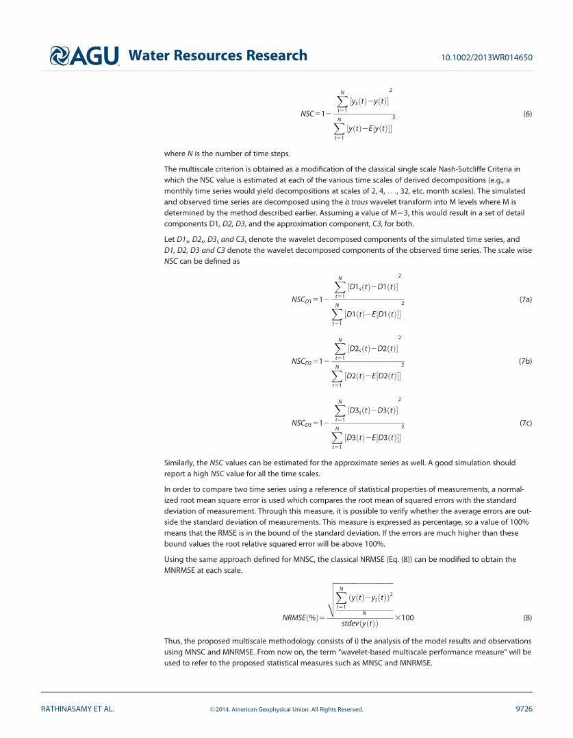
4.1. Synthetic Time SeriesIn this, the first phase, the given daily streamflow time series of was sequentially corrupted with a range ofadded synthetic errors of known properties. These include (i) error in the form of a systematic under predic-tion, (ii) error in timing, applied in the form of a uniform shift of one time step, (iii) two different error mod-els obtained by adding persistence in the form of a long memory component, (iv) adding a trend and achange of slope of the trend to the existing time series, (v) scaling the peak flows above a defined thresholdby a factor of 0.7, (vi) error introduced by systematically under predicting process observations that fallbelow a defined threshold, and finally (vii) in this case study, two separate time series are generated bycombinations of time series obtained in (v) and (vi). The mathematical expressions for these different timeseries are shown in Table 2.

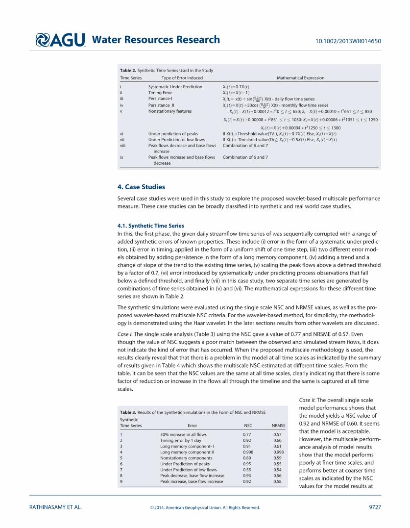
The synthetic simulations were evaluated using the single scale NSC and NRMSE values, as well as the pro-posed wavelet-based multiscale NSC criteria. For the wavelet-based method, for simplicity, the methodol-ogy is demonstrated using the Haar wavelet. In the later sections results from other wavelets are discussed.

Case i: The single scale analysis (Table 3) using the NSC gave a value of 0.77 and NRSME of 0.57. Eventhough the value of NSC suggests a poor match between the observed and simulated stream flows, it doesnot indicate the kind of error that has occurred. When the proposed multiscale methodology is used, theresults clearly reveal that that there is a problem in the model at all time scales as indicated by the summaryof results given in Table 4 which shows the multiscale NSC estimated at different time scales. From thetable, it can be seen that the NSC values are the same at all time scales, clearly indicating that there is somefactor of reduction or increase in the flows all through the timeline and the same is captured at all timescales.

Case ii: The overall single scalemodel performance shows thatthe model yields a NSC value of0.92 and NRMSE of 0.60. It seemsthat the model is acceptable.However, the multiscale perform-ance analysis of model resultsshow that the model performspoorly at finer time scales, andperforms better at coarser timescales as indicated by the NSCvalues for the model results at

Table 2. Synthetic Time Series Used in the Study

Time Series Type of Error Induced Mathematical Expression

i Systematic Under Prediction XsðtÞ50:7XðtÞii Timing Error XsðtÞ5Xðt21Þiii Persistance-I Xs(t)5 x(t) 1 sin 0:2pt

180

� �X(t) - daily flow time series

iv Persistance_II XsðtÞ5XðtÞ150cos 0:2pt60

� �X(t) - monthly flow time series

v Nonstationary features XsðtÞ5XðtÞ10:00012 � t20 � t � 650; Xs5XðtÞ10:00010 � t2651 � t � 850

XsðtÞ5XðtÞ10:00008 � t2851 � t � 1050; Xs5XðtÞ10:00006 � t21051 � t � 1250

XsðtÞ5XðtÞ10:00004 � t21250 � t � 1300vi Under prediction of peaks If X(t) >Threshold value(TV1), XsðtÞ50:7XðtÞ Else, XsðtÞ5XðtÞvii Under Prediction of low flows If X(t)< Threshold value(TV2), XsðtÞ50:5XðtÞ Else, XsðtÞ5XðtÞviii Peak flows decrease and base flows

increaseCombination of 6 and 7

ix Peak flows increase and base flowsdecrease

Combination of 6 and 7

Table 3. Results of the Synthetic Simulations in the Form of NSC and NRMSE

SyntheticTime Series Error NSC NRMSE

1 30% increase in all flows 0.77 0.572 Timing error by 1 day 0.92 0.603 Long memory component- I 0.91 0.614 Long memory component II 0.998 0.9985 Nonstationary components 0.89 0.596 Under Prediction of peaks 0.95 0.557 Under Prediction of low flows 0.55 0.548 Peak decrease, base flow increase 0.93 0.569 Peak increase, base flow increase 0.92 0.58



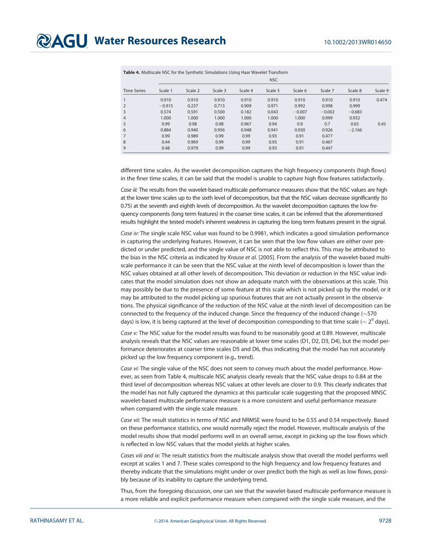
different time scales. As the wavelet decomposition captures the high frequency components (high flows)in the finer time scales, it can be said that the model is unable to capture high flow features satisfactorily.

Case iii: The results from the wavelet-based multiscale performance measures show that the NSC values are highat the lower time scales up to the sixth level of decomposition, but that the NSC values decrease significantly (to0.75) at the seventh and eighth levels of decomposition. As the wavelet decomposition captures the low fre-quency components (long term features) in the coarser time scales, it can be inferred that the aforementionedresults highlight the tested model’s inherent weakness in capturing the long term features present in the signal.

Case iv: The single scale NSC value was found to be 0.9981, which indicates a good simulation performancein capturing the underlying features. However, it can be seen that the low flow values are either over pre-dicted or under predicted, and the single value of NSC is not able to reflect this. This may be attributed tothe bias in the NSC criteria as indicated by Krause et al. [2005]. From the analysis of the wavelet-based multi-scale performance it can be seen that the NSC value at the ninth level of decomposition is lower than theNSC values obtained at all other levels of decomposition. This deviation or reduction in the NSC value indi-cates that the model simulation does not show an adequate match with the observations at this scale. Thismay possibly be due to the presence of some feature at this scale which is not picked up by the model, or itmay be attributed to the model picking up spurious features that are not actually present in the observa-tions. The physical significance of the reduction of the NSC value at the ninth level of decomposition can beconnected to the frequency of the induced change. Since the frequency of the induced change (�570days) is low, it is being captured at the level of decomposition corresponding to that time scale (� 29 days).

Case v: The NSC value for the model results was found to be reasonably good at 0.89. However, multiscaleanalysis reveals that the NSC values are reasonable at lower time scales (D1, D2, D3, D4), but the model per-formance deteriorates at coarser time scales D5 and D6, thus indicating that the model has not accuratelypicked up the low frequency component (e.g., trend).

Case vi: The single value of the NSC does not seem to convey much about the model performance. How-ever, as seen from Table 4, multiscale NSC analysis clearly reveals that the NSC value drops to 0.84 at thethird level of decomposition whereas NSC values at other levels are closer to 0.9. This clearly indicates thatthe model has not fully captured the dynamics at this particular scale suggesting that the proposed MNSCwavelet-based multiscale performance measure is a more consistent and useful performance measurewhen compared with the single scale measure.

Case vii: The result statistics in terms of NSC and NRMSE were found to be 0.55 and 0.54 respectively. Basedon these performance statistics, one would normally reject the model. However, multiscale analysis of themodel results show that model performs well in an overall sense, except in picking up the low flows whichis reflected in low NSC values that the model yields at higher scales.

Cases viii and ix: The result statistics from the multiscale analysis show that overall the model performs wellexcept at scales 1 and 7. These scales correspond to the high frequency and low frequency features andthereby indicate that the simulations might under or over predict both the high as well as low flows, possi-bly because of its inability to capture the underlying trend.

Thus, from the foregoing discussion, one can see that the wavelet-based multiscale performance measure isa more reliable and explicit performance measure when compared with the single scale measure, and the

Table 4. Multiscale NSC for the Synthetic Simulations Using Haar Wavelet Transform

Time Series

NSC

Scale 1 Scale 2 Scale 3 Scale 4 Scale 5 Scale 6 Scale 7 Scale 8 Scale 9

1 0.910 0.910 0.910 0.910 0.910 0.910 0.910 0.910 0.4742 20.915 0.237 0.713 0.909 0.971 0.992 0.998 0.9993 0.574 0.591 0.500 0.182 0.043 20.007 20.002 20.6834 1.000 1.000 1.000 1.000 1.000 1.000 0.999 0.9325 0.99 0.98 0.98 0.967 0.94 0.9 0.7 0.65 0.456 0.884 0.940 0.956 0.948 0.941 0.930 0.926 22.1667 0.99 0.989 0.99 0.99 0.93 0.91 0.4778 0.44 0.969 0.99 0.99 0.93 0.91 0.4679 0.48 0.979 0.99 0.99 0.93 0.91 0.447



former measure also provides an overall idea and understanding of the kind of error involved in thesimulation.

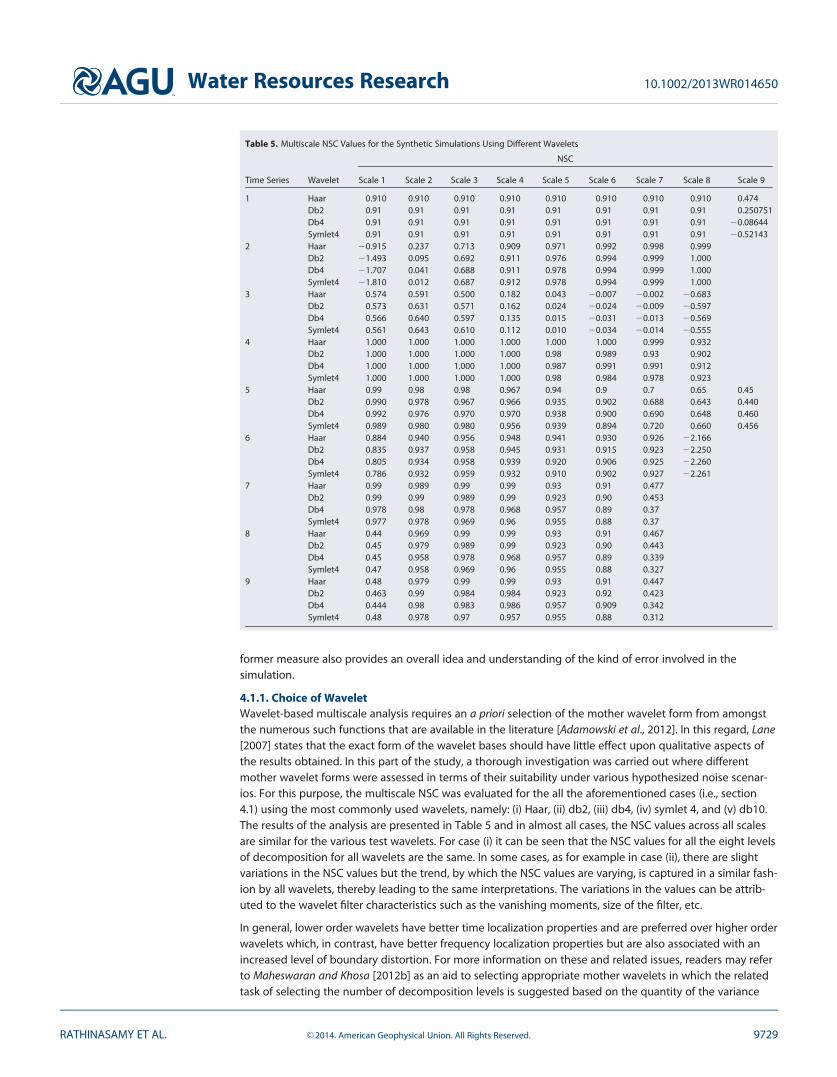
4.1.1. Choice of WaveletWavelet-based multiscale analysis requires an a priori selection of the mother wavelet form from amongstthe numerous such functions that are available in the literature [Adamowski et al., 2012]. In this regard, Lane[2007] states that the exact form of the wavelet bases should have little effect upon qualitative aspects ofthe results obtained. In this part of the study, a thorough investigation was carried out where differentmother wavelet forms were assessed in terms of their suitability under various hypothesized noise scenar-ios. For this purpose, the multiscale NSC was evaluated for the all the aforementioned cases (i.e., section4.1) using the most commonly used wavelets, namely: (i) Haar, (ii) db2, (iii) db4, (iv) symlet 4, and (v) db10.The results of the analysis are presented in Table 5 and in almost all cases, the NSC values across all scalesare similar for the various test wavelets. For case (i) it can be seen that the NSC values for all the eight levelsof decomposition for all wavelets are the same. In some cases, as for example in case (ii), there are slightvariations in the NSC values but the trend, by which the NSC values are varying, is captured in a similar fash-ion by all wavelets, thereby leading to the same interpretations. The variations in the values can be attrib-uted to the wavelet filter characteristics such as the vanishing moments, size of the filter, etc.

In general, lower order wavelets have better time localization properties and are preferred over higher orderwavelets which, in contrast, have better frequency localization properties but are also associated with anincreased level of boundary distortion. For more information on these and related issues, readers may referto Maheswaran and Khosa [2012b] as an aid to selecting appropriate mother wavelets in which the relatedtask of selecting the number of decomposition levels is suggested based on the quantity of the variance

Table 5. Multiscale NSC Values for the Synthetic Simulations Using Different Wavelets

Time Series Wavelet

NSC

Scale 1 Scale 2 Scale 3 Scale 4 Scale 5 Scale 6 Scale 7 Scale 8 Scale 9

1 Haar 0.910 0.910 0.910 0.910 0.910 0.910 0.910 0.910 0.474Db2 0.91 0.91 0.91 0.91 0.91 0.91 0.91 0.91 0.250751Db4 0.91 0.91 0.91 0.91 0.91 0.91 0.91 0.91 20.08644Symlet4 0.91 0.91 0.91 0.91 0.91 0.91 0.91 0.91 20.52143

2 Haar 20.915 0.237 0.713 0.909 0.971 0.992 0.998 0.999Db2 21.493 0.095 0.692 0.911 0.976 0.994 0.999 1.000Db4 21.707 0.041 0.688 0.911 0.978 0.994 0.999 1.000Symlet4 21.810 0.012 0.687 0.912 0.978 0.994 0.999 1.000

3 Haar 0.574 0.591 0.500 0.182 0.043 20.007 20.002 20.683Db2 0.573 0.631 0.571 0.162 0.024 20.024 20.009 20.597Db4 0.566 0.640 0.597 0.135 0.015 20.031 20.013 20.569Symlet4 0.561 0.643 0.610 0.112 0.010 20.034 20.014 20.555

4 Haar 1.000 1.000 1.000 1.000 1.000 1.000 0.999 0.932Db2 1.000 1.000 1.000 1.000 0.98 0.989 0.93 0.902Db4 1.000 1.000 1.000 1.000 0.987 0.991 0.991 0.912Symlet4 1.000 1.000 1.000 1.000 0.98 0.984 0.978 0.923

5 Haar 0.99 0.98 0.98 0.967 0.94 0.9 0.7 0.65 0.45Db2 0.990 0.978 0.967 0.966 0.935 0.902 0.688 0.643 0.440Db4 0.992 0.976 0.970 0.970 0.938 0.900 0.690 0.648 0.460Symlet4 0.989 0.980 0.980 0.956 0.939 0.894 0.720 0.660 0.456

6 Haar 0.884 0.940 0.956 0.948 0.941 0.930 0.926 22.166Db2 0.835 0.937 0.958 0.945 0.931 0.915 0.923 22.250Db4 0.805 0.934 0.958 0.939 0.920 0.906 0.925 22.260Symlet4 0.786 0.932 0.959 0.932 0.910 0.902 0.927 22.261

7 Haar 0.99 0.989 0.99 0.99 0.93 0.91 0.477Db2 0.99 0.99 0.989 0.99 0.923 0.90 0.453Db4 0.978 0.98 0.978 0.968 0.957 0.89 0.37Symlet4 0.977 0.978 0.969 0.96 0.955 0.88 0.37

8 Haar 0.44 0.969 0.99 0.99 0.93 0.91 0.467Db2 0.45 0.979 0.989 0.99 0.923 0.90 0.443Db4 0.45 0.958 0.978 0.968 0.957 0.89 0.339Symlet4 0.47 0.958 0.969 0.96 0.955 0.88 0.327

9 Haar 0.48 0.979 0.99 0.99 0.93 0.91 0.447Db2 0.463 0.99 0.984 0.984 0.923 0.92 0.423Db4 0.444 0.98 0.983 0.986 0.957 0.909 0.342Symlet4 0.48 0.978 0.97 0.957 0.955 0.88 0.312



explained by the decomposition. The decomposition is continued until the variance explained by the wave-let decomposition drops down significantly after a particular level of decomposition.

4.2. Real World Case Studies4.2.1. Case Study IFor the real world case study, SWAT model [Arnold et al., 1998; Neitsch et al., 2002] based basin-scale runoffsimulations were analyzed. SWAT is a well known watershed scale model that functions on a daily timestep, and is primarily applied to predict and evaluate long-term impacts of land cover and land manage-ment practices on the quantity and quality of runoff generated by watersheds with a dominant agriculture-based water use. The model is physically based and relies on environmental parameters and plant growthpotential to estimate the amount of water available in the landscape to contribute to the delivery of streamflow, sediment, nutrients, and pesticides to the watershed outlet. The SWAT model was selected for thisstudy because, on account of its free availability, it has acquired a large user base and is also being activelysupported and developed.

In this case study, five of the most sensitive parameters from a calibrated SWAT model were modified oneat a time and also in combination, and the performance measure of the models were evaluated using theproposed multiscale performance. The results were noted based on a total set of 20 simulations. Throughthis study, a direct relationship was attempted between the parameter of the model and the time scale atwhich their effect is most significant. The methodology was implemented for the Wainganga catchment–atributary of the Godavari River in India. The Wainganga rises in the Seoni district on the southern slopes ofthe Satpura Range of Madhya Pradesh (India), and drains an area of 58,500 km2 between latitudes 19�30’Nand 22�40’N and longitudes 78�0’E and 81�0’ E. After joining with the Wardha River, the united stream isknown as Pranahita, which ultimately falls into the Godavari River. The geographical location of the basin isshown in Figure 1. The SWAT model was set up and calibrated manually as detailed in Table 6. The modelyielded a NSC value equal to 0.87 and R2 50.88 for the calibration set, while the validation yielded a simi-larly high NSC value equal to 0.85. The model set up was used for generating different model simulationswith altered parameter values. Table 7 shows the altered parameters in each of the simulations. Table 8gives the single scale NSC and NRMSE for the different model simulations and the corresponding alteredparameters, while Table 9 shows the multiscale performances using the Haar wavelet for each of the SWAT

Figure 1. Location of Wainganga Basin.



simulations under altered parameter conditions. An examination of these results clearly shows the effectthat an incremental change in parameter values has on the model performance at that time scale at whichthe physical process governed by the parameter occurs.

For example, the parameters such as GW_DELAY, and GW_REVAMP, correspond to the groundwater contri-bution and the base flow. The base flows/low flows have a low frequency feature and therefore, the effectof changing them is appropriately captured in the coarser time scales corresponding to 6 months to 1 year.Similarly, parameter CN_F controls the peak flow (quick flow) of the catchment and thereby contributes tothe peak values in the hydrograph. The peak flows have a relatively higher frequency and a sharply tran-sient nature, and therefore the effect is seen to be captured at finer scales. It can be seen that the increaseor decrease in the ALPHA_B value affects the model performance at coarser scales and is in line with theunderstanding that ALPHA_B controls the base flow contribution and any change in its value will bereflected as a change in the long-term behavior of the system. Altering GWQMN in the model is seen toaffect the model performance at finer scales, indicating that the ability of the model to pick up peak flowsgets compromised, leading to the conclusion that the parameter GWQMN controls the peak flow. It is seen,therefore, that with the aid of the aforementioned simulations, parameters of the SWAT model may belinked to the multiscale performance measures leading to an easier and a more meaningful modelcalibration.

4.2.2. Case Study IIIn this case study, the effectiveness of the proposed multiscale performance measure was tested on theSind river basin in India. The river originates on the Malwa Plateau in Vidisha district (India) and flows North-Northeast through the districts of Guna, Ashoknagar, Shivpuri, Datia, Gwalior and Bhind in Madhya Pradeshto join the Yamuna River near Etawah (UP), just after the confluence of the Chambal River with the YamunaRiver (Figure 2). The Sind has a total length of 470 kilometres out of which a stretch of 461 kilometres lies inMadhya Pradesh and the remaining 9 kilometres falls in the state of Uttar Pradesh (UP). The monthly streamflow data from the period of 1981–1990 were used for calibration, while 1991–1999 was used for validation.

The model was calibrated based on the NSC and RMSE values, yielding a NSC value equal to 0.64. The modelresults are plotted in Figure 3. Visually, from the plots, it appears that the model performance is good with the

Table 6. Calibrated SWAT Model Parameters for Wainganga Basin

Symbol Description Unit Min. Max. Process Calibrated Values

ALPHA BF Base flow recession coefficient Days 0 1 Groundwater 0.9CN fa Curve number % 225 15 Surface runoff 3ESCO Soil evaporation coefficient 0.001 1 Evapotranspiration 0.4GW DELAY Groundwater delay time Day 1 500 Groundwater 90GW REVAP Revap coefficient 0.02 0.2 Groundwater 0.2GWQMN Depth of water in shallow aquifer mm 0 5000 Groundwater 10OV N Manning’s N 0.1 0.3 Overland flow 0.293SFTMP Snowfall temperature �C 25 5 SnowSLOPEa Slope % 20.5 1 Surface runoff 0.582SLSUBBSNa Slope subbasin % 20.5 1 Surface runoff 20.5SOL AWCa Available water capacity % 20.3 2 Groundwater, evaporation 1.31SOL Ka Saturated hydraulic conductivity % 20.5 1 Groundwater 0.02SURLAG Surface lag Day 1 12 Surface runoff 1

aThese parameters were changed as a percentage of their default values to maintain heterogeneity.

Table 7. Generation of Different Simulations From the Calibrated SWAT Model by Altering Parameters––Wainganga Basin

Simulation SURLAG ALPHA_B GW_DELA GW_REVA GWQMN ESCO OV_N SLOPE SLSUBBS CN_F

1 X2 X3 X4 X5 X6 X7 X8 X9 X X10 X X



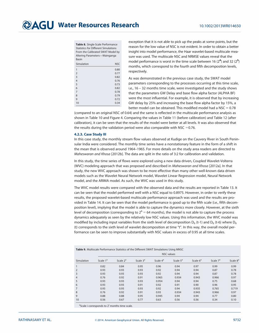
exception that it is not able to pick up the peaks at some points, but thereason for the low value of NSC is not evident. In order to obtain a betterinsight into model performance, the Haar wavelet-based multiscale mea-sure was used. The multiscale NSC and NRMSE values reveal that themodel performance is worst in the time scale between 16 (24) and 32 (25)months, which correspond to the fourth and fifth decomposition levels,respectively.

As was demonstrated in the previous case study, the SWAT modelparameters corresponding to the processes occurring at this time scale,i.e., 16 – 32 months time scale, were investigated and the study showsthat the parameters GW Delay and base flow alpha factor (ALPHA BF)were the most influential. For example, it is observed that by increasingGW delay by 25% and increasing the base flow alpha factor by 15%, abetter model can be obtained. This modified model had a NSC 5 0.78

(compared to an original NSC of 0.64) and the same is reflected in the multiscale performance analysis asshown in Table 10 and Figure 4. Comparing the values in Table 11 (before calibration) and Table 12 (aftercalibration), it can be seen that the results of the model were better at all levels. It was also observed thatthe results during the validation period were also comparable with NSC 50.76.

4.2.3. Case Study IIIIn this case study, the monthly stream flow values observed at Kudige on the Cauvery River in South Penin-sular India were considered. The monthly time series have a nonstationary feature in the form of a shift inthe mean that is observed around 1964–1965. For more details on the study area readers are directed toMaheswaran and Khosa [2012b]. The data are split in the ratio of 3:2 for calibration and validation.

In this study, the time series of flows were explored using a new data driven, Coupled Wavelet-Volterra(WVC) modeling approach that was proposed and described in Maheswaran and Khosa [2012a]. In thatstudy, the new WVC approach was shown to be more effective than many other well-known data drivenmodels such as the Wavelet Neural Network model, Wavelet Linear Regression model, Neural Networkmodel, and the ARIMA model. As such, the WVC was used in this study.

The WVC model results were compared with the observed data and the results are reported in Table 13. Itcan be seen that the model performed well with a NSC equal to 0.8975. However, in order to verify theseresults, the proposed wavelet-based multiscale performance approach was used and the results are pro-vided in Table 14. It can be seen that the model performance is good up to the fifth scale (i.e., fifth decom-position level), implying that the model is able to capture the dynamics more closely. However, at the sixthlevel of decomposition (corresponding to 26 5 64 months), the model is not able to capture the processdynamics adequately as seen by the relatively low NSC values. Using this information, the WVC model wasmodified by including input variables from the sixth level of decomposition D6 (t-1) and D6 (t-6) where D6

(t) corresponds to the sixth level of wavelet decomposition at time ‘‘t’’. In this way, the overall model per-formance can be seen to improve substantially with NSC values in excess of 0.95 at all time scales.

Table 8. Single-Scale PerformanceStatistics for Different SimulationsFrom the Calibrated SWAT Model byAltering Parameters––WaingangaBasin

Simulation NSC

1 0.802 0.773 0.824 0.765 0.736 0.827 0.788 0.799 0.7210 0.34

Table 9. Multiscale Performance Statistics of the Different SWAT Simulations Using MNSC

Simulation

NSC values

Scale 1a Scale 2a Scale 3a Scale 4a Scale 5a Scale 6a Scale 7a Scale 8a

1 0.82 0.84 0.95 0.96 0.94 0.97 0.99 0.992 0.93 0.93 0.93 0.92 0.94 0.94 0.87 0.783 0.93 0.93 0.93 0.92 0.94 0.94 0.87 0.784 0.76 0.92 0.91 0.965 0.934 0.943 0.966 0.975 0.93 0.93 0.93 0.954 0.94 0.94 0.75 0.686 0.93 0.93 0.91 0.92 0.91 0.90 0.96 0.957 0.93 0.93 0.93 0.92 0.94 0.935 0.765 0.7198 0.76 0.92 0.91 0.93 0.934 0.943 0.966 0.979 0.88 0.88 0.95 0.945 0.94 0.94 0.77 0.8010 0.56 0.67 0.77 0.63 0.56 0.56 0.34 0.10

aScale i corresponds to 2i months time scale.



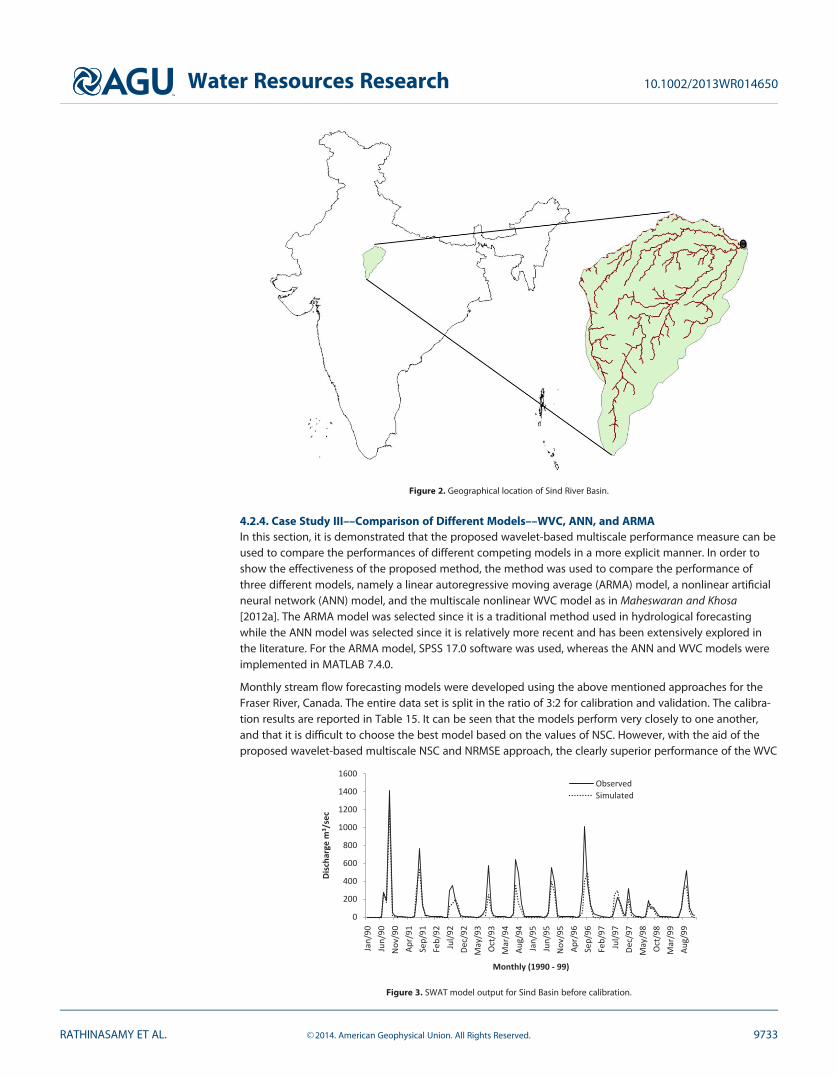
4.2.4. Case Study III––Comparison of Different Models––WVC, ANN, and ARMAIn this section, it is demonstrated that the proposed wavelet-based multiscale performance measure can beused to compare the performances of different competing models in a more explicit manner. In order toshow the effectiveness of the proposed method, the method was used to compare the performance ofthree different models, namely a linear autoregressive moving average (ARMA) model, a nonlinear artificialneural network (ANN) model, and the multiscale nonlinear WVC model as in Maheswaran and Khosa[2012a]. The ARMA model was selected since it is a traditional method used in hydrological forecastingwhile the ANN model was selected since it is relatively more recent and has been extensively explored inthe literature. For the ARMA model, SPSS 17.0 software was used, whereas the ANN and WVC models wereimplemented in MATLAB 7.4.0.

Monthly stream flow forecasting models were developed using the above mentioned approaches for theFraser River, Canada. The entire data set is split in the ratio of 3:2 for calibration and validation. The calibra-tion results are reported in Table 15. It can be seen that the models perform very closely to one another,and that it is difficult to choose the best model based on the values of NSC. However, with the aid of theproposed wavelet-based multiscale NSC and NRMSE approach, the clearly superior performance of the WVC

Figure 2. Geographical location of Sind River Basin.

0

200

400

600

800

1000

1200

1400

1600

Jan/90

Jun/90

Nov/90

Apr/91

Sep/91

Feb/92

Jul/92

Dec/92

May/93

Oct/93

Mar/94

Aug/94

Jan/95

Jun/95

Nov/95

Apr/96

Sep/96

Feb/97

Jul/97

Dec/97

May/98

Oct/98

Mar/99

Aug/99

Dis

char

ge m

3 /se

c

Monthly (1990 - 99)

Observed

Simulated

Figure 3. SWAT model output for Sind Basin before calibration.



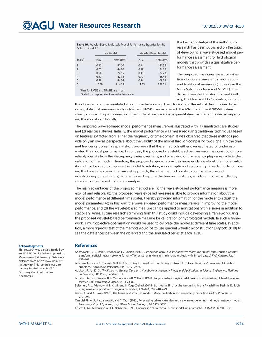
model compared to the ANN model becomes evident as is seen from Table 16. Further, it is seen that theANN-based approach does not fully capture the process dynamics at the fifth level. It is also evident thatthe performance of the latter ANN-based model is clearly inferior to the WVC model at all time scales andeven more so at higher time scales. It can be seen that the ANN model does not pick up some informationat higher time scales when compared to the WVC model. Thus, it can be seen that the proposed wavelet-based multiscale model performance measures can be used not only to analyze the performance of a sin-gle, stand alone model but that they are also useful when performance comparisons are required to bemade of multiple competing models which show ‘‘similar’’ performances on an overall basis, but are shownto be actually very different at some scale specific decomposition levels.

5. Summary and Discussion

The aim of this research was to propose a new performance measure for hydrological models based onwavelet analysis for reliable performance assessment of hydrological models. Different case studies relatedto hydrological modeling problems (i.e., poor performance in capturing low flows, peaks, time delay pres-ent, systematic under prediction, over prediction) were studied.

The case studies that were considered in this study showed that traditional measures of performance suchas NSC, NRMSE and RMSE are not sufficient and completely reliable for estimating hydrological model per-formance. These measures only provide an overall idea about the model performance; however, they donot provide any insight into the model.

In the case studies using synthetic time series, the NSC and NRMSE values did not provide any indication onthe sort of error in the simulations. Also, the single value of the NSC/NRMSE did not convey much informationregarding the model performance. In some of the cases, the analysis of the single scale NSC and NRMSE val-ues led to incorrect conclusions. In simulation 4 of the synthetic case study, the single scale NSC value wasfound to be 0.9981, which indicates a good performance of simulation in capturing the underlying features.However, it was seen that the low flow values were either over predicted or under predicted, and the NSCwas not able to reflect this. However, the proposed wavelet-based multiscale performance measure clearlypicked up the presence of the long frequency component in the time series picked up by the simulation.

From these different synthetic experiments, the following generic guidelines can be developed when usingthe proposed multi scale performance method:

1. If the NSC at the first and second level decompositions is low (<0.5),and the NSC for the remaining values are higher (>0.8), then thepeaks will be under predicted or over predicted, and all other featureswill likely be picked up well.

2. If the NSC at the higher level decompositions is low (<0.5), whereasthe NSC at the lower levels remains higher, this indicates that the lowflows might not be captured properly.

0

200

400

600

800

1000

1200

1400

1600

Jan/90

Jun/90

Nov/90

Apr/91

Sep/91

Feb/92

Jul/92

Dec/92

May/93

Oct/93

Mar/94

Aug/94

Jan/95

Jun/95

Nov/95

Apr/96

Sep/96

Feb/97

Jul/97

Dec/97

May/98

Oct/98

Mar/99

Aug/99

Dis

char

ge m

3 /se

cMonthly (1990 - 99)

Observed

Simulated

Figure 4. SWAT model output for Sind Basin after calibration with the aid of multiscale analysis.

Table 10. Single Scale Result Statis-tics for the SWAT Model for SindBasin

Result Statistics Value

RMSE(m3/s) 85.056NSC 0.64MAE(m3/s) 28.6151NRMSE(%) 64.6273



3. If there is a sudden low value of NSC (hence a higher valueof NRMSE) at the first level of decomposition whereas for allother levels there is a high NSC, then there might be a lagin the simulation. The lag is captured in the scale which cor-responds to the lag-period. For example, if the lag is of 1day, this is captured in the form of lower values of NSC andhigher values of NRMSE at the 1st level of decomposition.

4. If the NSC values are less than <0.5 at all levels, then themodel is not performing well at all time scales, and there-fore has to be calibrated for all parameters.

5. Also, the choice of wavelet does not affect the multiscaleperformance measure, however, care must be taken inusing the appropriate relationship between the scale ofthe given wavelet and the Fourier period.

In case study II, a connection was established between theSWAT model parameters and the corresponding time scalesat which these parameters affect the simulation. Using thisrelationship, the SWAT model calibration was made moremeaningful and easier. From case study III, it was observedthat the single performance measures do not aid in improv-ing the model. In the case of the physically based model, theperformance measures such as NSC and NRMSE only providethe numerical value indicating the reliability of the model;these do not help a modeller in improving the model. How-ever, using the proposed MNSC and MNRMSE provided infor-mation regarding at which scale the simulation did notmatch the observation. This information was then used tohelp modify the parameters of the model corresponding tothe physical processes at that scale.

From case study IV, it was seen that the proposed wavelet-based multiscale performance measure (MNSC, MNRMSE)was a more robust method in comparing two competingmodels compared to single scale measures. The proposedmethod was more reliable as it provides a scale by scaleanalysis, thereby making the comparison more meaningful.Furthermore, the NSC is biased because of high flows. Insome cases (simulation (iii) and (iv) of the synthetic casestudy) it was observed that even if the low flow is not cap-tured, the NSC values are still high; however, using the pro-posed multiscale method, the bias in the NSC is eliminated.Since the low flows and high flows are automatically sepa-rated using the Discrete Wavelet Transform, the multiscale

NSC is a more reliable estimate of the model performance.

In addition, single scale measures (e.g., NSC) are valid and meaningful only for stationary systems. For nonsta-tionary systems, the traditional model performance measures may under predict or over predict the perform-ance of the model. However, the wavelet transform can potentially convert a nonstationary time series intostationary components, and this can help in analysing nonstationary time series using the proposed method.

6. Conclusions

In this paper, an attempt was made to develop a quanti-tative wavelet-based multiscale measure for hydrologi-cal model performance analysis. Even though waveletshave been used for model performance assessments, to

Table 11. Multiscale Result Statistics for the SWATModel Simulations (Before Calibration) for SindBasin

Scalea NSC NRMSE(%)

1 0.38 78.252 0.66 58.243 0.78 46.024 0.32 81.975 0.29 84.116 0.018 99.09


Table 12. Multiscale Result Statistics for the SWATModel Simulations (After Calibration)––Sind Basin

Scalea NSC NRMSE(%)

1 0.58 64.252 0.68 55.443 0.785 46.004 0.65 59.975 0.59 57.116 0.28 49.09


Table 14. Multiscale Result Statistics for the WVCModel––Cauvery Basin

Scalea NSC NRMSE(%)

1 0.97 0.0652 0.99 0.153 0.99 0.4814 0.96 4.305 0.90 30.686 20.28 113.217 0.83 40.96

aScale i corresponds to 2i months time scale

Table 13. Single-Scale Result Statistics for theWVC Model––Cauvery Basin

Result Statistics Value

RMSE(m3/s) 49.3264NSC 0.9875MAE(m3/s) 44.3823NRMSE(%) 11.1633

Table 15. Single-Scale Model Performance Statistics forthe Different Models

Model NSC MAE(m3/s) NRMSE(%)

ARMA 0.74 582.98 48.9Neural Network Model 0.78 512.28 43.7Wavelet Volterra Model 0.80 482.2 41.8



the best knowledge of the authors, noresearch has been published on the topicof developing a wavelet-based model per-formance assessment for hydrologicalmodels that provides a quantitative per-formance assessment.

The proposed measures are a combina-tion of discrete wavelet transformationand traditional measures (in this case theNash-Sutcliffe criteria and NRMSE). Thediscrete wavelet transform is used (with,e.g., the Haar and Db2 wavelets) on both

the observed and the simulated stream flow time series. Then, for each of the sets of decomposed timeseries, statistical measures such as NSC and NRMSE are estimated. The MNSC and the MNRSME valuesclearly showed the performance of the model at each scale in a quantitative manner and aided in improv-ing the model significantly.

The proposed wavelet-based model performance measure was illustrated with (1) simulated case studiesand (2) real case studies. Initially, the model performance was measured using traditional techniques basedon features extracted from either the frequency or time domain. It was observed that these methods pro-vide only an overall perspective about the validity of the model through comparing two signals in the timeand frequency domains separately. It was seen that these methods either over estimated or under esti-mated the model performance. In contrast, the proposed wavelet-based performance measure could morereliably identify how the discrepancy varies over time, and what kind of discrepancy plays a key role in thevalidation of the model. Therefore, the proposed approach provides more evidence about the model valid-ity and can be used to improve the model. In addition, no assumption of stationarity is made for decompos-ing the time series using the wavelet approach; thus, the method is able to compare two sets ofnonstationary (or stationary) time series and capture the transient features, which cannot be handled byclassical Fourier-based coherence analysis.

The main advantages of the proposed method are: (a) the wavelet-based performance measure is moreexplicit and reliable; (b) the proposed wavelet-based measure is able to provide information about themodel performance at different time scales, thereby providing information for the modeler to adjust themodel parameters; (c) in this way, the wavelet-based performance measure aids in improving the modelperformance; and (d) the wavelet-based measure can be applied to nonstationary time series in addition tostationary series. Future research stemming from this study could include developing a framework usingthe proposed wavelet-based performance measure for calibration of hydrological models. In such a frame-work, a multiobjective optimization would be used to calibrate the model at different time scales. In addi-tion, a more rigorous test of the method would be to use gradual wavelet reconstruction [Keylock, 2010] tosee the differences between the observed and the simulated series at each level.

ReferencesAdamowski, J., H. Chan, S. Prasher, and V. Sharda (2012), Comparison of multivariate adaptive regression splines with coupled wavelet

transform artificial neural networks for runoff forecasting in Himalayan micro-watersheds with limited data, J. Hydroinformatics, 3,731–744.

Adamowski, J., and A. Prokoph (2014), Determining the amplitude and timing of streamflow discontinuities: A cross wavelet analysisapproach, Hydrological Processes, 28(5), 2782–2793.

Addison, P. S., (2010), The Illustrated Wavelet Transform Handbook: Introductory Theory and Applications in Science, Engineering, Medicineand Finance, CRC Press, London, U. K.

Arnold, J. G., R. Srinivasan, R. S. Muttiah, and J. R. Williams (1998), Large area hydrologic modeling and assessment part I: Model develop-ment, J. Am. Water Resour. Assoc., 34(1), 73–89.

Belayneh, A., J. Adamowski, B. Khalil, and B. Ozga-Zielinski(2014), Long-term SPI drought forecasting in the Awash River Basin in Ethiopiausing wavelet-support vector regression models, J. Hydrol., 508, 418–429.

Beven, K., and A. Binley (1992), The future of distributed models: Model calibration and uncertainty prediction, Hydrol. Processes, 6,279–298.

Campisi-Pinto, S., J. Adamowski, and G. Oron (2012), Forecasting urban water demand via wavelet-denoising and neural network models.Case study: City of Syracuse, Italy, Water Resour. Manage., 26, 3539–3558.

Chiew, F., M. Stewardson, and T. McMahon (1993), Comparison of six rainfall-runoff modelling approaches, J. Hydrol., 147(1), 1–36.

Table 16. Wavelet-Based Multiscale Model Performance Statistics for theDifferent Modelsa

Scaleb

NN Model Wavelet-Based Model

NSC NRMSE(%) NSC NRMSE(%)

1 0.16 91.66 0.34 81.322 0.80 44.18 0.87 36.193 0.94 24.65 0.95 22.234 0.82 42.18 0.79 45.445 0.29 84.34 0.54 68.186 23.60 214.39 21.25 150.01

aUnit for RMSE and NRMSE are m3/s.bScale i corresponds to 2i months time scale.

AcknowledgmentsThis research was partially funded byan INSPIRE Faculty Fellowship held byMaheswaran Rathinasamy. Data wereobtained from http://www.india-wris.nrsc.gov.in/. This research was alsopartially funded by an NSERCDiscovery Grant held by JanAdamowski.



http://www.india-wris.nrsc.gov.in/

http://www.india-wris.nrsc.gov.in/

Fugal, D. L. (2009), Conceptual Wavelets in Digital Signal Processing: An In-depth, Practical Approach for the Non-Mathematician, Space andSignals Technol. LLC, San Diego, Calif.

Grossmann, A., and J. Morlet (1984), Decomposition of Hardy functions into square integrable wavelets of constant shape, SIAM J. Math.Anal., 15(4), 723–736.

Houghton-Carr, H., (1999), Assessment criteria for simple conceptual daily rainfall-runoff models, Hydrol. Sci. J., 44(2), 237–261.Jiang, X., and S. Mahadevan (2011), Wavelet spectrum analysis approach to model validation of dynamic systems, Mech. Syst. Signal Pro-

cess., 25(2), 575–590.Keylock, C. J. (2010), Characterising the structure of nonlinear systems using gradual wavelet reconstruction, Nonlinear Processes Geophys.,

17, 615–632.Keylock, C. J. (2012), A resampling method for generating synthetic hydrological time series with preservation of cross correlative structure

and higher order properties, Water Resour. Res., 48, W12521, doi:10.1029/2012WR011923.Krause, P., D. P. Boyle, and F. Base (2005), Comparison of different efficiency criteria for hydrological model assessment, Adv. Geosci., 5(5),

89–97.Lane, S. N. (2007), Assessment of rainfall-runoff models based upon wavelet analysis, Hydrol. Processes, 21, 586–607.Lane, S. N., J. Chandler, and K. Richards (1994), Developments in monitoring and modelling small-scale river bed topography, Earth Surf.

Processes Landforms, 19, 349–368.Liu, Q., S. Islam, I. Rodriguez-Iturbe, and Y. Le (1998), Phase-space analysis of daily streamflow: Characterization and prediction, Adv. Water

Resour., 21(6), 463–475.Maheswaran, R., and R. Khosa (2012a), Wavelet Volterra coupled model for monthly stream flow forecasting, J. Hydrol., 450, 320–335.Maheswaran, R., and R. Khosa (2012b), Comparative study of different wavelets for hydrologic forecasting, Comput. Geosci., 46, 284–295.Maheswaran, R., J. Adamowski, and R. Khosa (2013), Multiscale streamflow forecasting using a new Bayesian model average based ensem-

ble multi-wavelet Volterra nonlinear method, J. Hydrol., 507, 186–200.McCuen, R. H., and W. M. Snyder (1975), A proposed index for comparing hydrographs, Water Resour. Res., 11(6), 1021–1024.Moeckel, R., and B. Murray (1997), Measuring the distance between time series, Physica D, 102(3–4), 187–194.Montanari, A., and E. Toth (2007), Calibration of hydrological models in the spectral domain: An opportunity for scarcely gauged basins?,

Water Resour. Res., 43, W05434, doi:10.1029/2006WR005184.Nalley, D., J. Adamowski, and B. Khalil (2012), Using discrete wavelet transforms to analyze trends in streamflow and precipitation in Que-

bec and Ontario (1954–2008), J. Hydrol., 475, 204–228.Nalley, D., J. Adamowski, B. Khalil, and B. Ozga-Zielinski (2013), Trend detection in surface air temperature in Ontario and Quebec, Canada

during 1967–2006 using the discrete wavelet transform, J. Atmos. Res., 132, 375–398.Nash, J., and J. Sutcliffe (1970), River flow forecasting through conceptual models part I: A discussion of principles, J. Hydrol., 10(3),

282–290.Neitsch, S., J. Arnold, J. Kiniry, R. Srinivasan, and J. Williams (2002), Soil and water assessment tool user’s manual version 2000, GSWRL Rep.

02-02, BRC Rep. 02–06, 438 pp., Tex. Water Resour. Inst., College Station.Nourani, V., A. Baghanam, J. Adamowski, and M. Gebremichael (2013), Using self-organizing maps and wavelet transforms for space-time

pre-processing of satellite precipitation and runoff data in neural network based rainfall-runoff modelling, J. Hydrol., 476, 228–243.Nourani, V., A. Baghanam, J. Adamowski, and O. Kisi (2014), Applications of hybrid wavelet-artificial intelligence models in hydrology: A

review, J. Hydrol., 514, 358–377.Percival, D. B. (2008), Analysis of geophysical time series using discrete wavelet transforms: An overview, in Nonlinear Time Series Analysis in

the Geosciences, edited by R. V. Donner and S. M. Barbosa, pp. 61-79, Springer, Berlin.Percival, D. B., and A. T. Walden (2000), Wavelet Methods for Time Series Analysis, Cambridge Univ. Press, Cambridge, U. K.Priestley, M. B. (1981), Spectral Analysis and Time Series, Academic, London, U. K.Schaefli, B., and H. V. Gupta (2007), Do Nash values have value?, Hydrol. Processes, 21(15), 2075–2080.Schaefli, B., and E. Zehe (2009), Hydrological model performance and parameter estimation in the wavelet-domain, Hydrol. Earth Syst. Sci.

Discuss., 6(2), 2451–2498.Shensa, M. (1992), The discrete wavelet transform: Wedding the a trous and Mallat algorithms, IEEE Trans. Signal Process., 40(10),

2464–2482.Takens, F. (1981), Detecting strange attractors in turbulence, in. Dynamical Systems and Turbulence, Lecture Notes in Mathematics, vol. 898,

edited by D. A. Rand and L.-S. Young, pp. 366–381, Springer, Berlin Heidelberg.Tiwari, M., and J. Adamowski (2013), Urban water demand forecasting and uncertainty assessment using ensemble wavelet-bootstrap-

neural network models, Water Resour. Res., 49, 6486–6507, doi:10.1002/wrcr.20517.Torrence, C., and G. P. Compo (1998), A practical guide to wavelet analysis, Bull. Am. Meteorol. Soc., 79(1), 61–78.von Hardenberg, J. G., F. Paparella, N. Platt, A. Provenzale, E. Spiegel, and C. Tresser (1997), Missing motor of on-off intermittency, Phys. Rev.

E, 55(1), 58.Whittle, P. (1953), The analysis of multiple stationary time series, J. R. Stat. Soc., Ser. B, 15 (1), 125–139.Willmott, C. J. (1982), Some comments on the evaluation of model performance, Bull. Amer. Meteor. Soc., 63, 1309–1313.



http://dx.doi.org/10.1029/2012WR011923

http://dx.doi.org/10.1029/2006WR005184

http://dx.doi.org/10.1002/wrcr.20517

Documents

Wavelet‐based multiscale performance analysis: An … ARTICLE 10.1002/2013WR014650 Wavelet-based multiscale performance analysis: An approach to assess and improve hydrological models