WAVELET ESTIMATION AND DEBUBBLING USING MINIMUM

ENTROPY DECONVOLUTION AND TIME DOMAIN LINEAR INVERSE

METHODS,

by

SHLOMO LEVY

B.Sc,, University of C a l i f o r n i a Los Angeles, 1977

A THESIS SUBMITTED IN PARTIAL FULFILLMENT OF THE

REQUIREMENTS FOR THE DEGREE OF MASTER OF SCIENCE

in

THE FACULTY OF GRADUATE STUDIES

(Department of Geophysics and Astronomy)

We accept t h i s thesis as conforming to

the required standard:

THE UNIVERSITY OF BRITISH COLUMBIA.

June, 1979

(c) Shlomo Levy, 1979

I n p r e s e n t i n g t h i s t h e s i s i n p a r t i a l f u l f i l m e n t o f t h e r e q u i r e m e n t s f o r

an a d v a n c e d d e g r e e a t t h e U n i v e r s i t y o f B r i t i s h C o l u m b i a , I a g r e e t h a t

t h e L i b r a r y s h a l l make i t f r e e l y a v a i l a b l e f o r r e f e r e n c e and s t u d y .

I f u r t h e r a g r e e t h a t p e r m i s s i o n f o r e x t e n s i v e c o p y i n g o f t h i s t h e s i s

f o r s c h o l a r l y p u r p o s e s may be g r a n t e d by t h e Head o f my D e p a r t m e n t o r

by h i s r e p r e s e n t a t i v e s . I t i s u n d e r s t o o d t h a t c o p y i n g o r p u b l i c a t i o n

o f t h i s t h e s i s f o r f i n a n c i a l g a i n s h a l l n o t be a l l o w e d w i t h o u t my

w r i t t e n p e r m i s s i o n .

D e p a r t m e n t n f GtOPHyZlCS 4»J> 4<Teo*/nMV

The U n i v e r s i t y o f B r i t i s h C o l u m b i a 2075 W e s b r o o k P l a c e V a n c o u v e r , C a n a d a V6T 1W5

D a t e APC-- IS " t<\7^

ABSTRACT

A new and d i f f e r e n t approach to the solution of the normal

equations of minimum entropy deconvolution (MED) i s developed,.

This approach which uses singular value decomposition i n the

i t e r a t i v e solution of the MED equations increases the si g n a l - t o -

noise r a t i o of the deconvolved output and enhances the

resolution of MEC*

The problem of deconvolution, and in p a r t i c u l a r wavelet

estimation, i s formulated as a l i n e a r inverse problem. Both

generalized l i n e a r inverse methods and Backus-Gilbert inversion

are considered. The proposed wavelet estimation algorithm uses

the MED output as a f i r s t approximation to the earth response.

The approximated response and the observed seismograms serve as

an input to the inversion schemes and the outputs are the

estimated wavelets^ The remarkable performance of the l i n e a r

inverse schemes f o r cases of highly noisy data i s demonstrated.

A debubbling example i s used to show the completeness of

the l i n e a r inverse schemes. F i r s t the wavelet estimation part

was carried out and then the debubbling problem was formulated

as a generalized l i n e a r inverse problem which was solved using

the estimated wavelet*

This work demonstrates the power of the l i n e a r inverse

schemes when dealing with highly noisy data.

TABLE OF CONTENTS

ABSTRACT .......

TABLE OF CONTENTS , i i i

LIST OF TABLES v

LIST OF FIGURES v i

ACKNOWLEDGEMENTS i x

CHAPTER 1: I n t r o d u c t o r y Remarks , .....1

CHAPTER 2: MED Using Matrix S p e c t r a l Decomposition

I n t r o d u c t i o n ....5

Theory 6

Examples: .....11

1. Example A: Tapered Ricker wavelet, 2.5% random

noise-

2. Example B: 25% white n o i s e

C o n c l u s i o n .............20

CHAPTER 3: Wavelet E s t i m a t i o n as a L i n e a r Inverse Problem

I n t r o d u c t i o n ......22

Theory: C o n v o l u t i o n as a Linear Inverse Problem 26

1. General L i n e a r i n v e r s e

2. B a c k u s - G i l b e r t i n v e r s i o n

P r a c t i c a l Notes 38

Examples: 40 i

1. Example A: Good q u a l i t y MED output

2. Example B: Low q u a l i t y MED output

3. Example C: S y n t h e t i c seismogram

Con c l u s i o n .......59

CHAPTER 4: Debubbling as a Generalized Linear Inverse

Problem.

Introduction ....62

Source Signature Estimation and Debubbling ............65

Examples: .....72

1. Example A: Synthetic seismogram

2. Example B: F i e l d example

Conclusion ..85

REFERENCES 88

L I S T O P T A B L E S

V

L I S T O P T A B L E S

I Model c h a r a c t e r i s t i c s f o r c a l c u l a t i o n of s y n t h e t i c seismograms. .........72

v i

LIST OF FIGURES

CHAPTER 1

1. Three liguid. layer model. 2

2. Source wavelet, impulse response and the corresponding

seismogram. .. 3

CHAPTER 2

1. Input for the f i r s t MED example. 13

2. Output of the f i r s t MED example. 14

3. Inverse operators of the f i r s t MED example

f i l t e r s . ...15

4. Input for the second MED example.1 .................. 17

5. Output of the second MED example. 18

6. Inverse operators of the second MED example

f i l t e r s 19

CHAPTER 3

1. Input and output of MED. 24

2. Input matrix for a discrete convolution problem. ...27

3. MED output for the smallest model inversion ...32

4. Kernels of the smallest model inversion. 32

5. MED output and the kernels for f l a t t e s t model

inversion. ..................<............ ..36

6. Input traces for the f i r s t l i n e a r inverse schemes

example , 41

7. MED output for the f i r s t example. . . 42

8. F i r s t estimated wavelets of the f i r s t example 44

9- Second estimated wavelets of the f i r s t example. ....46

10. Noisy input trace (second example) and i t s MED

output. 48

11. Plots of error versus number of eigenvalues l e f t

out of the solution of the second example. 49

12. Wavelets which were estimated by the generalized

l i n e a r inverse f o r the second example. 52

13. Wavelets which were estimated by the f l a t t e s t model

inversion for the second example. ......53

14. Model for synthetic seismogram generation. ........54

15. Source wavelet, synthetic seismogram and the MED

output 55

16. Plots of error versus number of eigenvalues l e f t

out of the solution of the synthetic seismogram

example. 57

17. Output wavelets of the inversion schemes for the

synthetic seismogram example. 58

CHAPTEE 4

1. Flow diagram of the debubbling procedure , 65

2. Basic pulse, compound wavelet signature and the

output of a convolution of a short MED

f i l t e r and the compound wavelet. ...69

3. Sketch of bubble pulse events.. ..................... 71

4. Sketch of r e f l e c t i o n events. 71

5. Layer model for synthetic seismogram ca l c u l a t i o n s . .74

6. Source wavelet signature for synthetic seismogram

generation -. 74

7. Synthetic seismograms based on the model of

Figure 5 75

8. Debubbled synthetic seismograms. ................... 77

9. Six traces from a r e f l e c t i o n p r o f i l e recorded o f f

Vancouver Island. 79

10. MED output of the traces of Figure 9. 80

11. Basic pulse signatures and example of source

signature used in the debubbling scheme. ........... 82

12. The traces of Figure 9 after debubbling.. 84

ix

ACKNOWLEDGEMENTS

I would l i k e to express my gratitude to my supervisor

Dr. R.M. Clowes for his encouragement, help and constructive

remarks during every stage of the work.

For his most stimulating course on l i n e a r inverse methods

which triggered the larger part of thi s work as well as for his

most helpful suggestions and remarks I wish to express my thanks

to Dr. D.W. Oldenburg.

My deepest thanks to Dr..T.J. Ulrych for his stimulating

discussions and suggestions which led to a large part of t h i s

work.

Special thanks go to my friend Mr. C.J. Walker f o r his

help and suggestions.

Synthetic seismograms were generated by computer program

STPSYN written by E.A. Wiggins and D.V. Helmberger.

Funding f o r thi s project was provided through operating

grant A7707 of the Natural Sciences and Engineering Research

Council Canada and research grant from the Dniversity of B r i t i s h

Columbia. Additional funds were donated by Mobil O i l Canada

Ltd., Shell Canada Resources Ltd. and Chevron Standard Ltd.

1

CHAPTER 1

I n t r o d u c t o r y Remarks

Seismic methods are commonly used t o a i d the study of the

earth's i n t e r i o r . Employing the assumption of a l a y e r e d e a r t h ,

one uses the f a c t t h a t on p a s s i n g from one l a y e r t o another the

energy of an e l a s t i c wave i s separated i n t o a t r a n s m i t t e d and

r e f l e c t e d component. The amount of energy r e f l e c t e d or

r e f r a c t e d i s b a s i c a l l y a f u n c t i o n of the angle of i n c i d e n c e o f

the wave at the i n t e r f a c e and the a c o u s t i c impedance ( d e n s i t y

times v e l o c i t y ) of both l a y e r s . A geophone placed on the

e a r t h ' s s u r f a c e responds t o t h i s r e f l e c t e d and r e f r a c t e d energy

and i t s output, a f t e r a m p l i f i c a t i o n , i s recorded (the

seismogram). The task o f the s e i s m o l o g i s t i s t o i n t e r p r e t the

seismogram. That i s , the s e i s m o l o g i s t i s l o o k i n g f o r the

g e o l o g i c a l model of the subsurface which can be i n f e r r e d from

the seismogram.

To make t h i n g s c l e a r e r , c o n s i d e r the f o l l o w i n g example;

Assume a t h r e e l a y e r model as shown i n F i g u r e 1 . For s i m p l i c i t y

l e t these be l i q u i d l a y e r s (no shear waves), with d e n s i t y and

v e l o c i t y as shown i n F i g u r e 1 , and the c o n d i t i o n ^ V j < > ^ sv

a .

Neglect the d i r e c t wave and assume t h a t only r e f l e c t e d energy

corresponding t o the rays 1 and 2 i n F i g u r e 1 has been recorded

on the seismogram.

Define two time s e r i e s : 1 ) the source wavelet, which

re p r e s e n t s the shape of the s i g n a l before i t was t r a n s f e r r e d

2

F i g u r e 1

Three l i q u i d l a y e r model

t h r o u g h t h e ground; 2) the i m p u l s e response s e r i e s . The l a t t e r

i s a time s e r i e s which c o n s i s t s o f z e r o s everywhere e x c e p t f o r

the t i m e s which c o r r e s p o n d e x a c t l y t o the a r r i v a l t i m e s o f

r e f l e c t e d o r r e f r a c t e d energy. For t h e s e p a r t i c u l a r t i m e s , the

i m p u l s e r e s p o n s e becomes a s p i k e w i t h an a m p l i t u d e which

r e f l e c t s t h e energy l e f t i n the s i g n a l a f t e r t r a v e l l i n g t h e path

s p e c i f i e d by the p a r t i c u l a r r a y .

Assume t h a t the s o u r c e w a v e l e t i s a P i c k e r w a v e l e t , and

u s i n g the model o f F i g u r e 1 , t h e c o r r e s p o n d i n g i m p u l s e response

can be d e r i v e d . F i g u r e 2 shows t h i s time s e r i e s t o g e t h e r w i t h

3

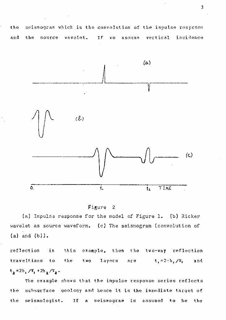
the seismogram which i s the c o n v o l u t i o n of the impulse response

and the source wavelet. I f ve assume v e r t i c a l i n c i d e n c e

T

i,

ro

Figure 2

(a) Impulse response f o r the model of Figure 1. (b) Ricker

wavelet as source waveform. (c) The seismogram (convolution of

(a) and (b)).

r e f l e c t i o n i n t h i s example, then the two-way r e f l e c t i o n

t r a v e l t i m e s to the two l a y e r s are t,=2'h,/V, and

t A = 2 h , /V, • 2 h i / V 4 .

The example shows t h a t the impulse response s e r i e s r e f l e c t s

the s u b s u r f a c e geology and hence i t i s the immediate t a r g e t of

the s e i s m o l o g i s t . I f a seismogram i s assumed t o be the

4

c o n v o l u t i o n of a source wavelet with the e a r t h ' s response, then

i d e n t i f y i n g and d e r i v i n g the impulse response f u n c t i o n i s termed

"d e c o n v o l u t i o n " .

This work i s devoted t o t h e de c o n v o l u t i o n problem i n

ge n e r a l and, i n p a r t i c u l a r , to the debubbling problem. T h i s i s

a s p e c i a l case of the g e n e r a l deconvolution problem which a r i s e s

under p a r t i c u l a r p h y s i c a l c o n d i t i o n s . To s o l v e these problems,

minimum entropy d e c o n v o l u t i o n and l i n e a r i n v e r s i o n t e c h n i q u e s

are developed.

5

CHAPTER 2

M i n i m u m E n t r o p y D e c o n v o l u t i o n U s i n g , M a t r i x S p e c t r a l

D e c o m p o s i t i o n ^

I N T R O D U C T I O N

The c o n c e p t o f m i n i m u m e n t r o p y d e c o n v c l u t i o n w h i c h was

i n t r o d u c e d b y W i g g i n s (1977) p r e s e n t s a u s e f u l t o o l t o a i d

s e i s m i c i n t e r p r e t a t i o n . T h i s d e c o n v o l u t i o n t e c h n i q u e s e a r c h e s

f o r a f i l t e r F w h i c h , when c o n v o l v e d w i t h a n i n p u t s i g n a l X ,

w i l l c o n v e r t t h a t s i g n a l t o an o u t p u t Y w h i c h h a s a " s i m p l e "

a p p e a r a n c e .

(1) Y = X * F

w h e r e * d e n o t e s c o n v o l u t i o n .

W i g g i n s (1977) d e f i n e d " ' s i m p l e * t o mean t h a t e a c h d e s i r e d

s i g n a l c o n s i s t o f a f e w l a r g e s p i k e s o f u n k n o w n s i g n o r l o c a t i o n

s e p a r a t e d b y n e a r l y z e r o t e r m s " . A l t h o u g h i t i s a g o o d m e t h o d ,

MED p r o c e s s i n g t e n d s t o e n h a n c e l a r g e a m p l i t u d e i m p u l s e s

c o m p a r e d t o s m a l l e r a m p l i t u d e o n e s a n d t h e r e b y c a u s e s seme l o s s

o f v a l u a b l e i n f o r m a t i o n . A m o d i f i c a t i o n o f MED h a s b e e n

p r o p o s e d b y Ooe. a n d U l r y c h (1979) who i n t r o d u c e d t h e e x p o n e n t i a l

t r a n s f o r m a t i o n w i t h a m o d i f i e d s i m p l i c i t y n o r m . T h e y h a v e s h o w n

t h a t t h e i r a p p r o a c h p r o v i d e s a b a l a n c e b e t w e e n t h e n o i s e

s u p p r e s s i o n e f f e c t o f MED a n d t h e a b i l i t y t o r e c o v e r s m a l l

6

amplitude impulses.

In t h i s work we take the o r i g i n a l version of MED (Wiggins

1977) and improve i t s performance by using a d i f f e r e n t method of

solving the normal equations. In p a r t i c u l a r we assume that the

noisy components of the solution are mainly associated with the

small eigenvalues of the autocorrelation matrix. We write the

solution as a weighted summation of the eigenvectors of the

autocorrelation matrix and r e j e c t those components of the

solution which are associated with the smaller eigenvalues.

THEORY

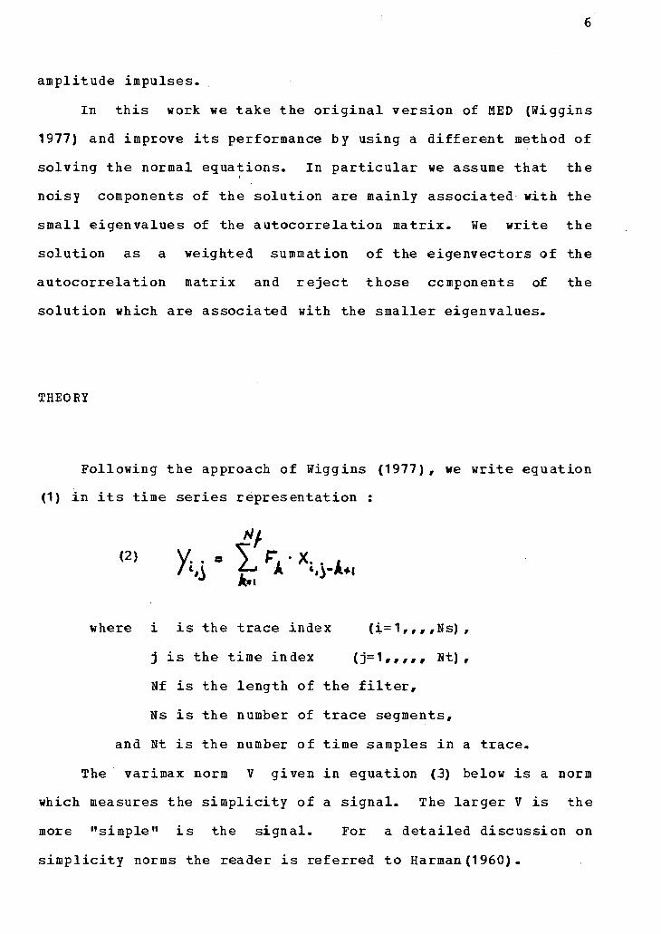
Following the approach of Wiggins (1977), we write equation

(1) i n i t s time series representation :

(2) y . . * S r. • x. . .

where i i s the trace index (i=1,, # /Ns),

j i s the time index (j=1#w#* Nt) ,

Nf i s the length of the f i l t e r ,

Ns i s the number of trace segments,

and Nt i s the number of time samples i n a trace.

The varimax norm V given i n eguation (3) below i s a norm

which measures the s i m p l i c i t y of a s i g n a l . The larger V i s the

more "simple" i s the signal. For a detailed discussion on

s i m p l i c i t y norms the reader i s referred to Harman (1960).

7

Since we are looking for the f i l t e r which w i l l maximize the

varimax (simplest possible appearance of the output t r a c e ) ; we

proceed by taking the gradient of V, set t i n g i t egual to zero

and solving :

0 " I §*; -

from eguation (2) we have:

substituting eguation (5) into ( 4 ) we get:

8

•» * J

which can be written in a matrix form as

(7) A-r*£ where

A i s a weighted autocorrelation matrix,

G i s a weighted crosscorrelation vector,

and F i s the vector of desired f i l t e r c o e f f i c i e n t s .

Equation (7) i s highly nonlinear but i t can be solved by

an i t e r a t i v e scheme. An i n i t i a l f i l t e r F" i s proposed and

convolved with the input series to give Y°. Through eguations

( 3 ) , (4a) and (6), the l a t t e r enables c a l c u l a t i o n of the

weighted crosscorrelation G°, and the weighted autocorrelation

matrix A°. Having G° and A°, we can solve for an updated

f i l t e r F 1 . Then the procedure can be repeated u n t i l the varimax

norm changes very l i t t l e with subseguent i t e r a t i o n s . Wiggins

(1977) used the Levinson recursion algorithm f o r the solution of

(7) in order to implement t h i s i t e r a t i v e procedure.

In t h i s paper, we take a different approach. The set of

eguations (7) i s solved by decomposition of matrix A into i t s

spectral components (Lanczos 1961), and finding i t s inverse.

For t h i s procedure A i s decomposed as shown below :

(8) A s K A R r

where R i s a matrix whose columns consist of the

eigenvectors of matrix A.

9

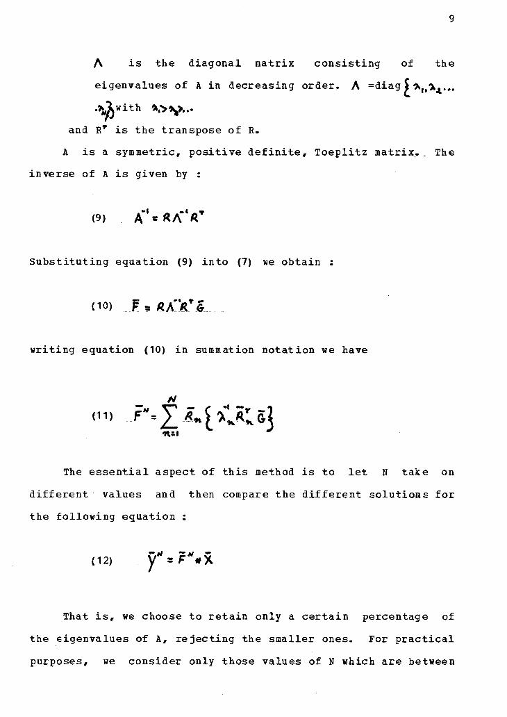
A i s the diagonal matrix consisting of the

eigenvalues of A i n decreasing order. A =diag £ * „ 0 ^ , . .

. ^ w i t h ft,^*^...

and E* i s the transpose of R.

A i s a symmetric, positive d e f i n i t e , Toeplitz matrix.. The

inverse of A i s given by :

(9) A M««A"*ft T

Substituting eguation (9) into (7) we obtain :

do) J * «A"'* TS

writing equation (10) i n summation notation we have

N

The e s s e n t i a l aspect of this method i s to l e t N take on

dif f e r e n t values and then compare the d i f f e r e n t solutions for

the following equation :

d 2 ) y" = F%X

That i s , we choose to retain only a cert a i n percentage of

the eigenvalues of A, rejecting the smaller ones. For p r a c t i c a l

purposes, we consider only those values of N which are between

10

0.2N^ to 0.8N^ where N̂ . i s the f i l t e r length. We consider

only these values since the varimax does not converge for very

small N and the solution of (12) looks very si m i l a r to the

o r i g i n a l MED output for large N. When N=N^, the solution of

(12) i s the same as the o r i g i n a l MED solution of Wiggins (1S77).

In applying the method we l e t N (the number of

eigenvalues used i n the solution) change over predetermined

i n t e r v a l s , take the solution of (12) with the smallest N value

as our reference, and plot the variance of a l l the other

possible solutions versus N . By variance we mean here the

sguare of the difference (Y* - Y*), where Y* i s the solution

of (12) corresponding to the smallest N value used. The

advantage of such a plot i s that i t t e l l s us how many possible

solutions we have that are s i g n i f i c a n t l y d i f f e r e n t . For short

f i l t e r lengths, i t i s probably best to plot a l l the output

solutions Y and examxne how those solutions change as a

function of N.

11

EXAMPLES

The examples which follow use single channel traces. These

are especially appropriate to our approach since matrix spectral

decomposition i s expensive computationally. For single channel

problems we may write eguation (6) as

* J •>

or

A*- * = &*

Since A* i s now independent of Y we w i l l have to f i n d the

spectral components of A* only once with consequent saving of

computer time. The examples discussed below were constructed i n

such a way that a complete recovery of the generating spike

sequence by the o r i g i n a l MED version was not possible, as w i l l

be shown.

Example A.

The wavelet, spike t r a i n and the r e s u l t i n g trace with 2.5%

added white noise i s shown i n Figure 1. The spacing of the

spikes compared to the wavelet length makes t h i s example a

p a r t i c u l a r l y d i f f i c u l t deconvolution problem. As stated in the

l a s t section, i t i s often useful to plot the variance of a l l

possible solutions versus N. Figure 2(a) shows such a plot but

12

i t i s not of much help i n t h i s p a r t i c u l a r example because the

f i l t e r length i s short and the number of solution models i s

small.

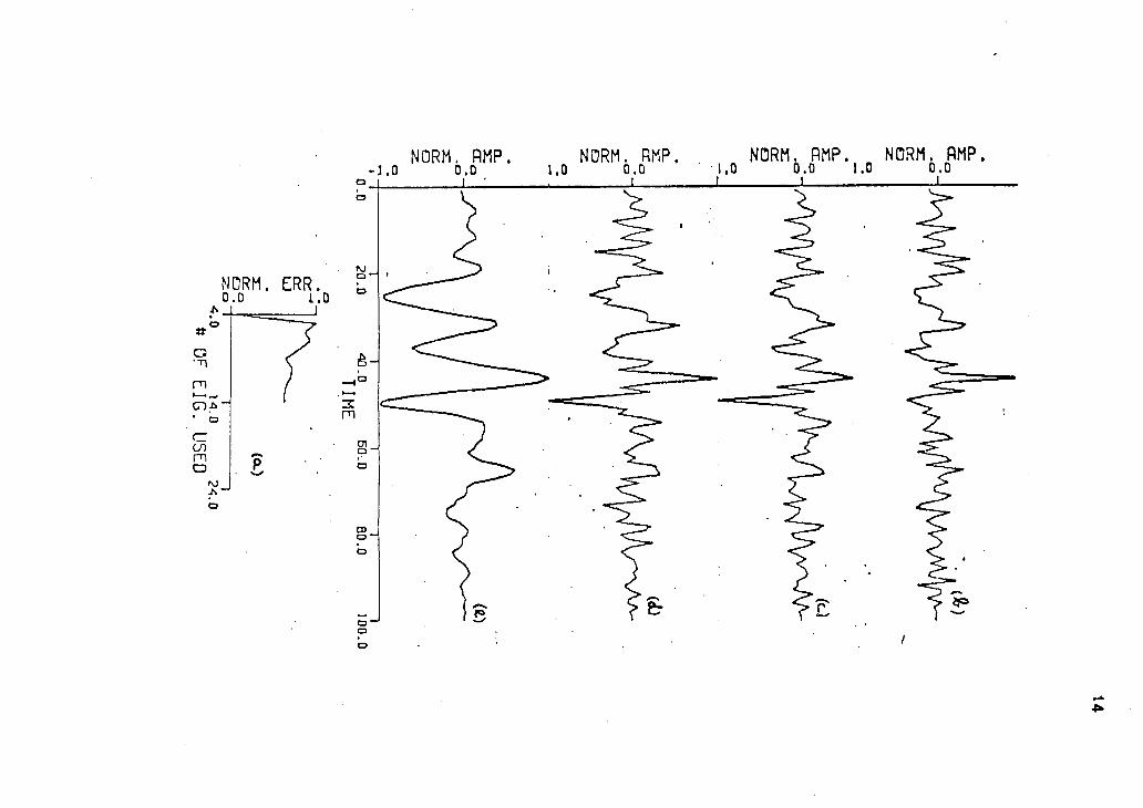
As shown i n Figure 2(b) the o r i g i n a l version of MED was

unable to recover the generating spike sequence. The spikes

become increasingly v i s i b l e as we rej e c t more and more

eigenvalues i n the construction of the f i l t e r solution (equation

(11)). Note the development of the output from Figure 2(c) to

Figure 2 (e). The l a t t e r does include a l l the input spikes shown

in Figure 1(b) but i t i s evident that the high freguency content

of the output decreases as more eigenvalues are dropped.

As shown i n Chapter 3 , the inverse of the MED f i l t e r i s the

wavelet i f i t i s assumed that the MED output i s the impulse

response. We t r i e d to recover the wavelet by finding the

inverse operator of the MED f i l t e r . For t h i s purpose we used

the optimum spiking algorithm of T r e i t e l and Robinson (1966).

The results are shown i n Figure 3 . The inverse of the MED

f i l t e r of the o r i g i n a l version did not give an acceptable

description of the input wavelet (compare Figure 3(a) with

Figure 1(a)). This r e s u l t was not surprising i n view of the

poor spike recovery of that f i l t e r . A s l i g h t improvment was

achieved by inverting the MED f i l t e r with N=8 (Figure 3 ( b ) ) , but

the estimated wavelet corresponding to the MED f i l t e r with N=5

i s t o t a l l y unacceptable even though we may consider Y s to be our

best output (compare Figure 2(e) with 1(b)). This i s e a s i l y

understood i n view of the clear differences i n freguency content

of the output sequences shown i n Figures 2(e) and 1(b).

1 3

\ i ( , — . p— , 0.0 20.0 40.0 SO.O 80.0 100.

TIME F i g u r e 1

(a) The g e n e r a t i n g wavelet W of example A .

(b) The s p i k e trace S from which the i n p u t t r a c e X of example A Was d e r i v e d .

(c) The i n p u t t r a c e X that i s the r e s u l t of the c o n v o l u t i o n of W with S plus 2.5% White n o i s e :

X=K*S + 2.5% white noise .

15a

Figure 2

(a) A plot of the variance versus N (the number of eigen­

values used i n the so l u t i o n ! . The f i l t e r length i s 14.

(b) The solution corresponding to N 14, which i s i d e n t i c a l

with the o r i g i n a l MED solution of Wiggins (1977).

(c) The solution corresponding to N 13.

(d) The solution corresponding to N 8".

( e ) The solution corresponding to N 5.

I I 1 1 0.0 20.0 40.0 60.0

TIKE Figure 3.

(a) The inverse of the MED f i l t e r corresponding to

(b) The inverse of the MED f i l t e r corresponding to N=8.

(c) The inverse of the MED f i l t e r corresponding to N=5.

16

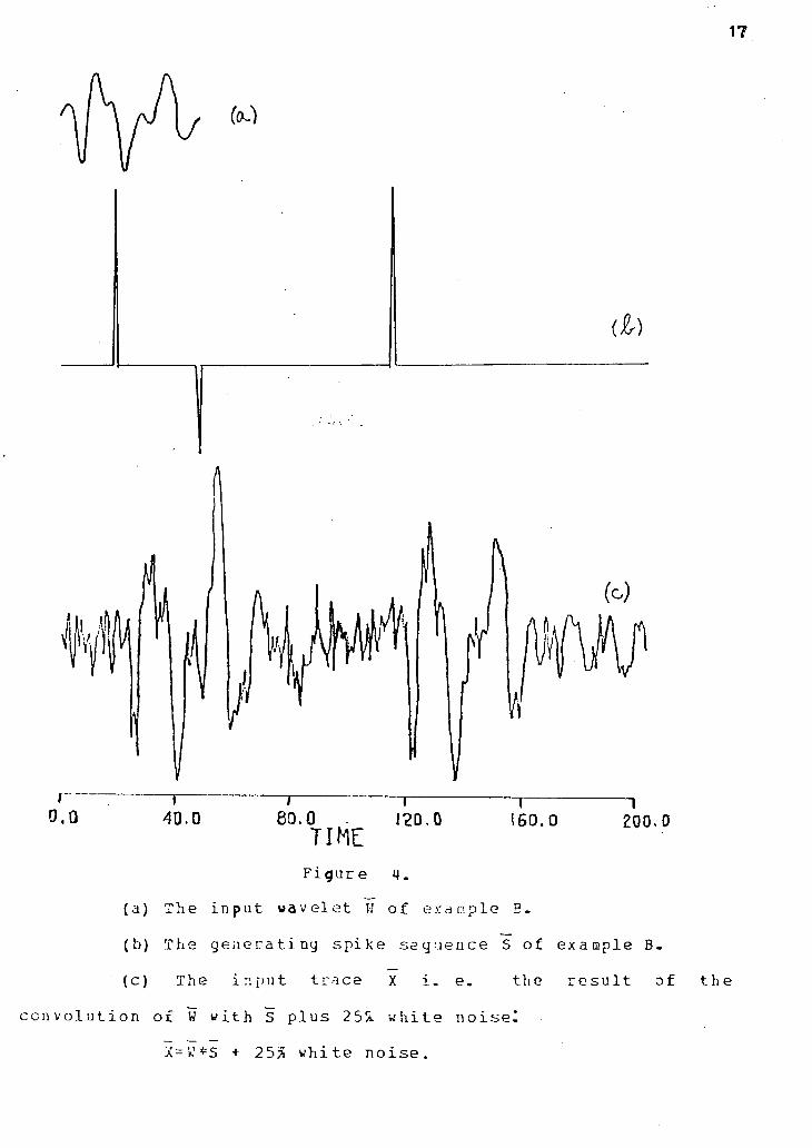
Example B.

In t h i s example we used a somewhat more complicated wavelet

(Figure 4(a)) to generate the synthetic input trace. This

wavelet was convolved with the spike sequence of Figure 4(b) and

25% white noise was added. The resultant input trace i s shown

in Figure 4(c). Although there i s wavelet overlap i n t h i s

example the main obstacle i s the high percentage of white ncise.

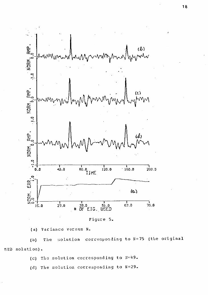
The plot of the variance versus the number of eigenvalues

used i n the construction of the MED f i l t e r (Figure 5(a)) proved

useful i n t h i s example i n which we l e t N take the values

N=15+2n, n=0,1,....r30. It i s clear from the plot that there

are only three s i g n i f i c a n t l y d i f f e r e n t solutions to eguation

(12) for t h i s example. These correspond to the f l a t regions

between the pairs of arrows.

As shown i n Figure 5(b), the o r i g i n a l MED solution did not

give a complete recovery of the generating spike seguence.

However as we rej e c t more and more eigenvalues i n the

construction of the MED f i l t e r a cle a r improvement i s v i s i b l e .

The output Y 2 9 (Figure 5(d)) does include a l l the generating

spikes although i t s frequency content i s much lcwer than that of

the generating spike sequence, as noted before. The r e l a t i v e

amplitudes of the recovered sequence shown i n Figure 5(d), match

very well with those of the input spike seguence shown i n Figure

4(b) .

Figure 6 shows the inverses of the f i l t e r s used to derive

Figures 5(b), (c) and (d) . When compared with Figure 4(a), i t

i s clear that the source wavelet was not reproduced. This i s

due to two causes : (1) when large numbers of eigenvalues are

17

r -0,0 40.0

(I)

~1 I

80.0 120.0 T I M E

ISO.O I

2 0 0 . 0

F i g u r e 4 .

(a) The i n p u t w a v e l e t H o f e x a m p l e B.

(b) The g e n e r a t i n g s p i k e s e q u e n c e S o f e x a m p l e B .

(c) The i n p u t t r a c e x i . e. t h e r e s u l t o f t h e

c o n v o l u t i o n o f W w i t h S p l u s 25% w h i t e n o i s e !

X=W*S + 25% w h i t e n o i s e .

1 8

-CD '

CL.

c c 0

on

0 . 0 " B O . O TJME

~l 1 2 0 . 0

U J

o 1 i 1 1 5 . 0 2 7 . 0 3 9 . 0 5 1 . 0

* OF E I G . USED

~T 1 B 0 . 0

—I 2 0 0 . 0

to

6 3 . 0 7 5 . 0

F i g u r e 5.

(a) V a r i a n c e v e r s u s N.

(b) The s o l u t i o n c o r r e s p o n d i n g to 11 = 75 ( t h e o r i g i n a l

MED s o l u t i o n ) -

(c) The s o l u t i o n c o r r e s p o n d i n g to N=*)9-

(d) The s o l u t i o n c o r r e s p o n d i n g to N=29.

20

used, the exact spike seguence has not been reproduced; and (2)

when small numbers of eigenvalues are used, the freguency

content of the output i s much lower than that cf the true spike

seguence (although Figure 5(d) c l e a r l y shows the impulse

response) .

CONCLUSION

(a) Singular value decomposition applied to the i t e r a t i v e

solution of the MED eguations increases the signal-to-noise

r a t i o of the deconvolved output and enhances the resolution of

the MED approach.

(b) It i s commonly known that those eigenvectors associated

with the small eigenvalues have more zero crossings than those

which are associated with the large eigenvalues (Wiggins et a l

1976). Hence we expect that for a smaller N we would get a

lower freguency f i l t e r F and hence the output Y w i l l contain

lower frequencies. This point i s readily observed i n examples A

and B.

(c) The minimum value of N i s determined by the varimax i n

the sense that for F to be an acceptable f i l t e r , the varimax

must converge. Then the smallest possible N i s the smallest N

for which the varimax i n the i t e r a t i v e solution described above

does converge .

(d) The f i l t e r length i s of e s s e n t i a l importance i n MED

problems. The best f i l t e r length for our MED algorithm i s the

one that gives the most acceptable r e s u l t i n the o r i g i n a l MED

21

version. An approach to t h i s

discussed by Olrych et a l (1979).

(e) Inversion of the MED

algorithm w i l l not i n general

estimate.

problem has recently been

f i l t e r r e s u l t i n g from our

give an acceptable wavelet

2 2

CHAPTER 3

Wavelet Estimation as a Linear Inverse Problem

INTRODUCTION

The problem of wavelet estimation i s one of ess e n t i a l

importance i n seismic deconvolution. It i s commonly assumed

that a seismogram can be modelled as the convolution of a

seismic wavelet with the earth response- Since the earth

response r e f l e c t s the subsurface geology i t i s one of the icain

targets of seismic data processing. Given a seismic wavelet,

one may deconvolve the seismogram to get the earth's response.

Variations of the deconvolution problem are common i n land and

marine data processing. An example i s the debubbling problem

(Wood et a l 1978) which we w i l l treat i n Chapter 4. Lines and

Ulrych (1977) have summarized the current approaches to wavelet

estimation. Such technigues include the Weiner-Levinson double

inverse method and Wold-Kolmogorov f a c t o r i z a t i o n , both of which

use the assumptions of an impulse response that i s a white noise

seguence and of a minimum phase wavelet. A more recent approach

- wavelet estimation by homomorphic deconvolution - does not use

these assumptions. However, i t does assumes that the wavelet

cepstrum i s read i l y separable from the cepstrum of the seismic

trace. (The cepstrum i s defined as the inverse transform of the

logarithm of the time sequence's Fourier transform.)

This work approaches the problem of wavelet estimation

23

using a combination of the techniques which are commonly applied

in linear inversion and the method of minimum entropy

deconvolution or MED (see Chapter 2 ) . The application of MED to

an input trace X w i l l y i e l d an output which consists of:

a. the spike sequence Y which i s the primary MED

output and

b. the MED f i l t e r (operator) F.

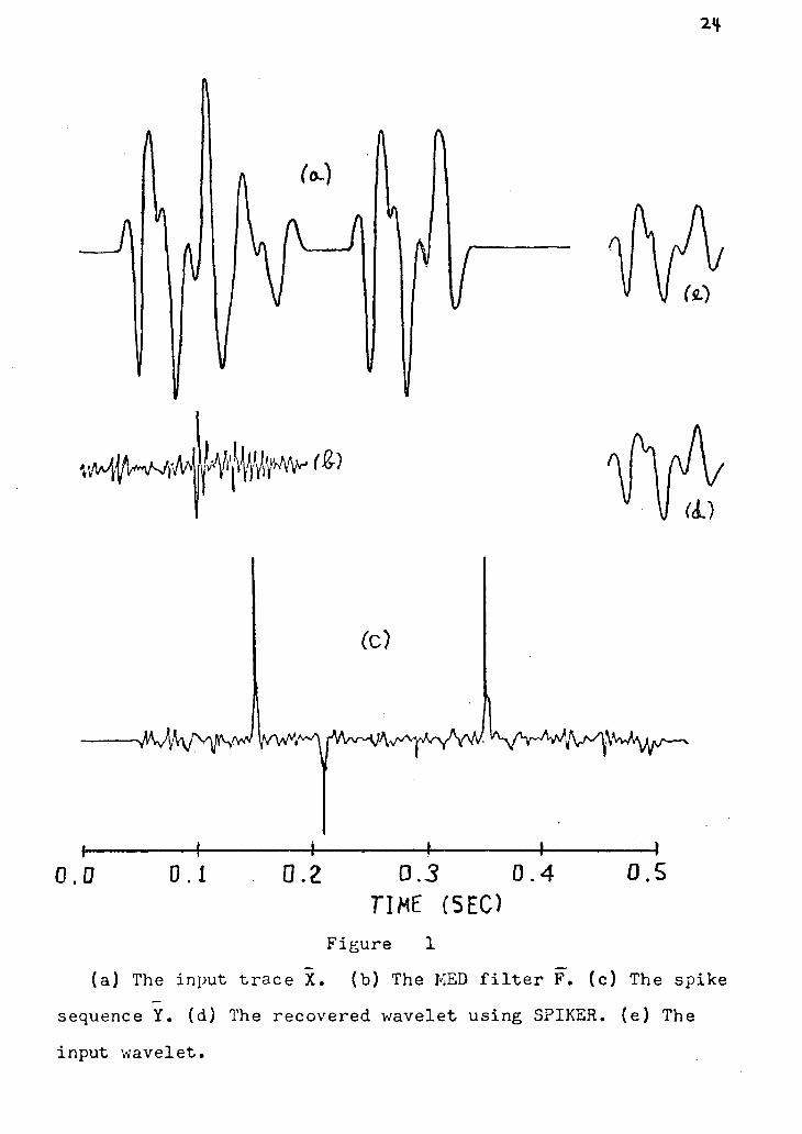
The time series represented by X, Y and F are related to each

other through the following eguation:

(1) X*F=Y

where * denotes convolution.

Figure 1 gives an example of three time series which follow the

r e l a t i o n described in equation (1) .

By convolving both sides of equation (1) with F-1=Wr we

get:

X*F*W=Y*W

or

(2) W*Y=X

If we assume that the time series Y i s a true representation of

the earth response then from eguation (2) , W i s the wavelet.

Eguation (2) indicates that i n order to find the wavelet we need

to f i n d the inverse of the MED operator.

One approach to doing t h i s i s to use the algorithm SPIKER

given by Robinson (1967). This algorithm i s designed to fi n d

the optimum inverse operator of a given time series ( T r e i t e l and

Robinson 1966). It gives good res u l t s on noiseless traces as

shown by Figure 1, (d) and (e).

However, the wavelet also can be estimated by formulating

2<f

0 . 0 D . l

CO

4-0 . 2 0 . 3 0 . 4

TIME ( S E C ) 0 . 5

Figure 1

(a) The input trace X. (b) The KED f i l t e r F. (c) The spike

sequence Y. (d) The recovered wavelet using SPIKER. (e) The

input wavelet.

25

eguation (2) as a generalized l i n e a r inverse problem or solving

the i n t e g r a l equivalent of eguation (2) using the Backus-Gilbert

approach. We assume here that the spiked minimum entropy

deconvolution output i s a f i r s t estimate of the earth response,

and use i t together with the observed seismic trace to extract

the wavelet. The generalized l i n e a r inverse approach i s a

parametric method and the solution wavelet w i l l be represented

by a set of parameters corresponding to discrete time values.

In the Backus-Gilbert approach the earth response, the observed

seismic trace, and the output wavelet are a l l continuous

functions of time . Both technigues allow the user t c control

the accuracy of the solution (see the section on P r a c t i c a l

Notes), a property which i s very important when dealing with

noisy data. In addition the Backus-Gilbert approach also allows

us to incorporate boundary conditions into the problem.

Since we assume that the MED output represents the earth

response, the guality of the estimated wavelet depends on the

quality of the computed impulse response ( i . e. MED output).

However, we w i l l show i n example B that by using l i n e a r inverse

methods a useful wavelet estimation can be extracted from

seemingly useless MED output.

26

THEORY : CONVOLUTION AS A LINEAR INVERSE PROBLEM

A. General Linear Inverse

We w i l l present here only those aspects of the general

l i n e a r inverse theory which are relevant to our problem. For

additional d e t a i l s concerning t h i s approach, the reader i s

referred to Wiggins (1972), Jackson (1972) or Wiggins et a l

(1976). The generalized linear inverse development follows

Wiggins et a l (1976).

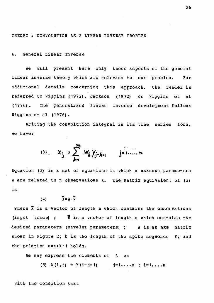
Writing the convolution i n t e g r a l i n i t s time series form,

we have:

Equation (3) i s a set of equations in which m unknown parameters

W are related to n observations X . The matrix equivalent of (3)

i s

(H) X = A - W

where 5 i s a vector of length n which contains the observations

(input trace) ; W i s a vector of length m which contains the

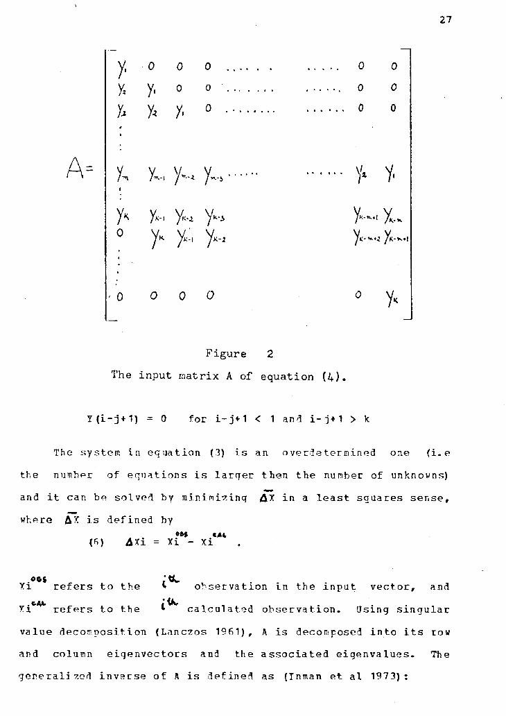
desired parameters (wavelet parameters) ; A i s an nxm matrix

shown i n Figure 2; k i s the length of the spike sequence Y; and

the r e l a t i o n n=m+k-1 holds.

We may express the elements of A as

(5) A(i,j) = Y(i-j+1) j = 1....m ; i=1. n

with the condition that

27

A*

0 0

y. y. 0

y, y< y.

0

0 0 0

y< y*. y * , y * *

0 y * y«:, y*. a

0 o

0 0 0 0 0 0

y < . ^ i y

y*-*».j yc

0 y«

F i g u r e 2

The i n p u t m a t r i x A of equation (4).

Y (i-j+1) = 0 for i-j+1 < 1 and i-j+1 > k

The system i n equation (3) i s an overdetermined one ( i . e

the number of equations i s l a r g e r then the number of unknowns)

and i t can be s o l v e d by minimizing AX i n a l e a s t squares sense,

where AX i s d e f i n e d by

(6) A X i = Xi - X i

X i r e f e r s t o the <• eft. ;1K

X i r e f e r s to the

o b s e r v a t i o n i n the i n p u t v e c t o r , and

' ~ c a l c u l a t e d o b s e r v a t i o n . Using s i n g u l a r

value decomposition (Lanczos 1961), A i s decomposed i n t o i t s row

and column e i g e n v e c t o r s and the a s s o c i a t e d e i g e n v a l u e s . The

g e n e r a l i z e d i n v e r s e o f A i s d e f i n e d as (Tnman et a l 1973):

28

<7> H^s A | Ul where

UT i s the transpose of 0 which consists of q eigenvectors

of length n associated with the column vectors of A ( i . e . the

data eigenvectors).

V consists of g eigenvectors of length m associated with

the row vectors of A (i.e the parameter eigenvectors).

A*' i s the inverse of A which consists of the g

eigenvalues of A i n descending order. A =diag £ fc,^...« a n <^ q i s the rank of A.

The solution to equation (4) i s then

(8) W*=H-X

W* i s the smallest solution (least euclidian length) that

minimizes IAX J 2 . The r e l a t i o n of W* to W can be obtained by

substituting equation (4) into (8) which gives

(9) W*= (H • A) • W=R. ?

The matrix E i s referred to as the resolution matrix (Inman et

a l 1973). If q=m, E i s the i d e n t i t y matrix; but i f q<m, the

resolution matrix i s no longer the i d e n t i t y matrix and %* i s a

weighted summation of the parameter eigenvectors used to

describe the wavelet.

The calculated observations < X C A L are determined from

(10) XCAt=A.W*

W* w i l l not be egual to W except for an i d e a l case ; hence

the vector AX = ( X°*S - X c A l ) w i l l not be the zero vector. As

a matter of f a c t , i n noisy cases we are net interested i n

reproducing the observations exactly since i f we do so the

29

errors i n the observations and/or the spike trace w i l l propagate

d i r e c t l y into the solution (wavelet). The power of l i n e a r

inversion i n t h i s p a r t i c u l a r problem i s that i t gives us the

a b i l i t y to control the accuracy of the solution. For example,

i n the case of a known noise l e v e l of ̂ % we are interested i n

a l l the models (wavelets) i n which :

(11) Max £ A X J ^ < <* % • Max £ X j ^ j=1 n

Thus the exact solution i s c e r t a i n l y not the only solution that

interests us and i t i s l i k e l y that i t w i l l not provide the best

estimate of the wavelet .

B. Backus-Gilbert Inversion

The basic assumptions required for the generalized l i n e a r

inverse problem - (1) MED output i s a true representation of the

earth response, and (2) the seismogram can be modelled as a

convolution of the earth response with the input wavelet - also

are applicable to the Backus-Gilbert inversion. That i s , we

assume that the observed seismic trace can be expressed d i r e c t l y

by the convolution i n t e g r a l

m

(12) X(tj) = ^ W(t) Y(tj-t) dt

where

X(tj) i s the datum corresponding to time t j .

W(t) i s the wavelet .

Y (t j-t) i s the spike trace (MED output) ; Y i s ccmmonly

referred to as the kernel.

In the case where the functions X(t) and/or Y(t) i n

30

equation (12) contain a certain amount of noise, we have some

f l e x i b i l i t y . Linear inverse theory allows us to choose a

solution model W (t) which w i l l reproduce the data X(t) to within

a desired standard deviation instead of solving (12) exactly.

This a b i l i t y i s the key which enables us to treat high noise

problems succesfully.

Define W(t) such that :

W(t) = W(t) t g (0,T)

W(t) = 0 t j (Q,T)

That i s , the wavelet has a f i n i t e length T. Using the

d e f i n i t i o n of the wavelet we can rewrite equation (12) as

T

(13) X(Tj) = ̂ W(t) Y(Tj-t) dt

9

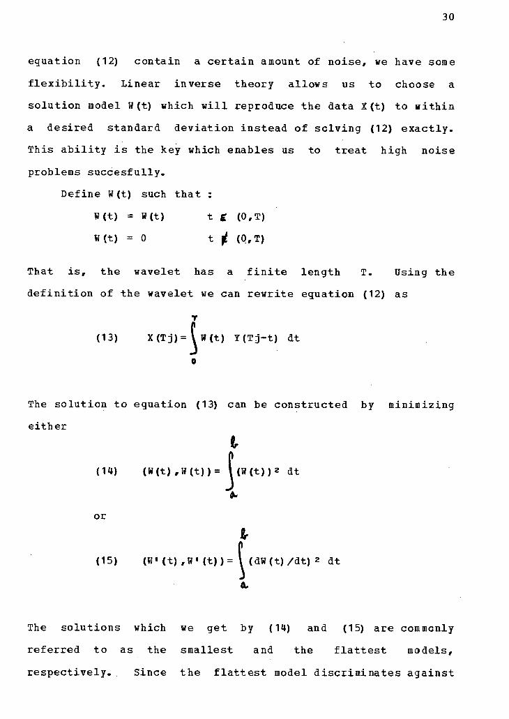
The solution to eguation (13) can be constructed by minimizing

either t

(14) (W(t) ,W(t))= ^(W(t))2 dt

or

I (15) (W« (t) ,W« (t))= ^ (dW(t) /dt) 2 dt

OL

The solutions which we get by (14) and (15) are commonly

referred to as the smallest and the f l a t t e s t models,

respectively. Since the f l a t t e s t model discriminates against

31

steep g r a d i e n t s , we expect i t w i l l ensure good behaviour of the

model i n the r e g i o n of i n t e r e s t .

1. S m a l l e s t Model

The k e r n e l s of eguation (12) are generated by the MED

output. Using the nomenclature Gj f o r the k e r n e l s we o b t a i n

(16) G j ( t ) = Y(tj-t+1) 1 ^tj-t+1< T

G j ( t ) = 0 1 >tj-t+1 and tj-t+1> T

Since the k e r n e l s must be a t l e a s t piecewise-continuous to allow

i n t e g r a t i o n , i t i s convenient t o assume t h a t Y i s c o n s t r u c t e d

from a s e r i e s of box c a r s of width At (otherwise a s p l i n e curve

f i t t i n g approximation should be used to give a proper continuous

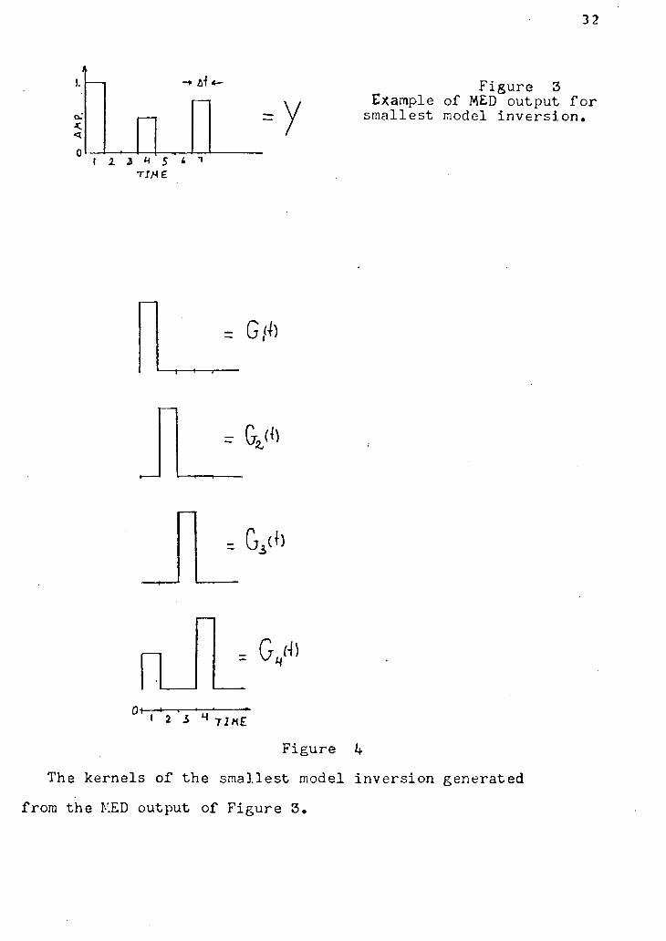
approximation of the MED o u t p u t ) . For example, suppose we have

the MED output shown i n F i g u r e 3:

Assume the wavelet i s of l e n g t h 4 (T=4) .

Then

G1 (t) =Y (1-t+1) t £ (0,4)

G2 (t) =Y(2-t + 1) t t (0,4)

G3 (t) =Y(3-t+1) t E(0,4)

G4(t) =Y(4-t+1) t £(0,4) e t c .

F i g u r e s 3 and 4 i l l u s t r a t e t h e r e l a t i o n between the k e r n e l s Gj

and the MED output Y as s p e c i f i e d i n eguation (16).

We assume t h a t the wavelet i s a l i n e a r combination of the

k e r n e l s :

3 2

F i g u r e 3 Example of MED output f o r

s m a l l e s t model i n v e r s i o n .

I X 3 H 5 * 1

-1 1 r -

0+-

- G &

1 2 5 H TIME

F i g u r e 4

The k e r n e l s o f the s m a l l e s t model i n v e r s i o n g e n e r a t e d

from the MED output of F i g u r e 3 .

33

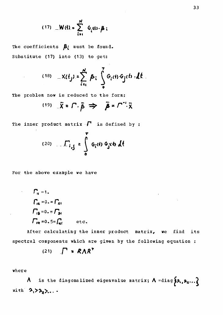
d7) _W(4L-5! 0,tu-y»i tai

The c o e f f i c i e n t s J&£ must be found.

Substitute (17) into (13) to get:

( V T

0 The problem now i s reduced to the form:

The inner product matrix /"* i s defined by : r

(20) r i # j a ^ G(.«) *j<4). it

For the above example we have

H,* =0. 5=/^ ( etc.

After c a l c u l a t i n g the inner product matrix, we f i n d i t s

spectral components which are given by the following equation :

(21) p * *ARr

where

A i s the diagonalized eigenvalue matrix; A =diag ^A t >5k A...^

with *,» 4>... -

34

B i s the eigenvector matrix , and

E T i s the transpose of E.

To compute the model we use

A /

( 2 2 ) _wi;»_j&'jLT» ( R A Y X J . M ^ ^ ) ;

""V b *̂ &^ , the basis functions, and o(j , the c o e f f i c i e n t s of the basis

functions, are given below .

(23)

and

(24)

Since the kernels can be described by a sum of step functions

the model also w i l l be a sum of step functions .

2. F l a t t e s t Model

To derive the " f l a t t e s t " model, the kernels (the MED output

Y) are assumed to be a series of functions . In t h i s case,

eguation (16) takes the form:

(16a)

0,t i s the d i g i t i z a t i o n i n t e r v a l of the MED output. Note the

35

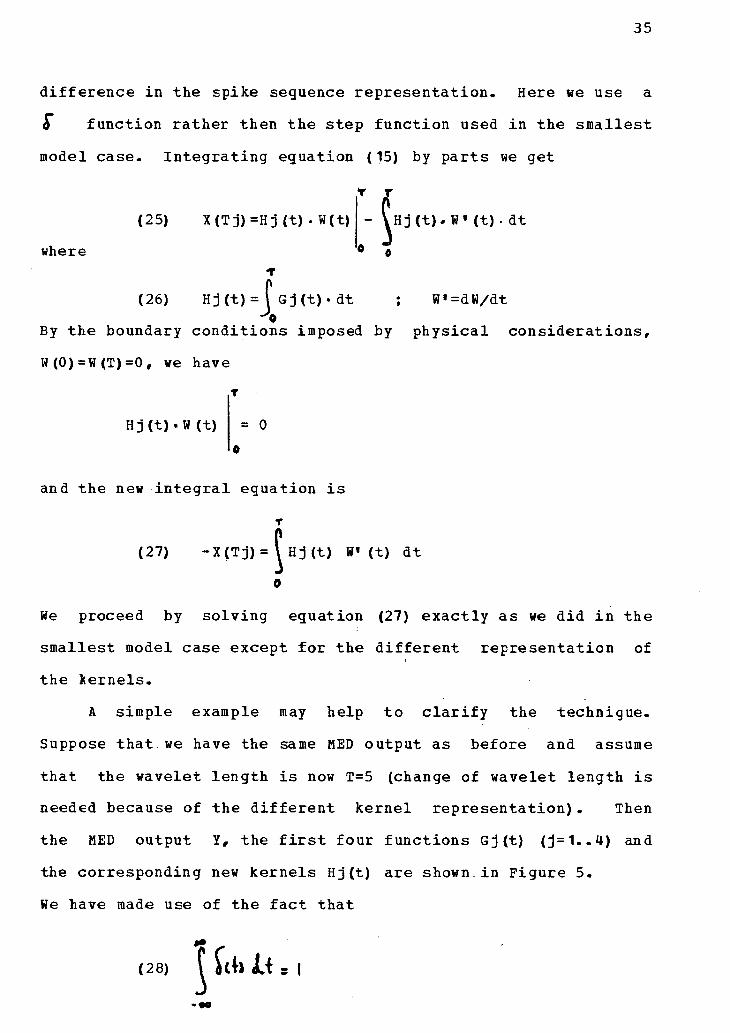
difference i n the spike sequence representation. Here we use a

J* function rather then the step function used i n the smallest

model case. Integrating equation (15) by parts we get

* r

(25) X(Tj)=Hj (t) . W(t) - ^ H j ( t ) . W (t) • dt

where 0 »

(26) Hj (t) = I G j ( t ) . dt ; W«=dW/dt

By the boundary conditions imposed by physical considerations,

W(0)=W(T)=0, we have T

Hj(t)«W(t) = 0

and the new i n t e g r a l eguation i s

T

(27) -X(Tj)= ^Hj(t) W» (t) dt

0

We proceed by solving equation (27) exactly as we did i n the

smallest model case except for the different representation of

the kernels.

A simple example may help to c l a r i f y the technigue.

Suppose that we have the same MED output as before and assume

that the wavelet length i s now T=5 (change of wavelet length i s

needed because of the d i f f e r e n t kernel representation). Then

the MED output Y, the f i r s t four functions Gj(t) (j=1..4) and

the corresponding new kernels Hj(t) are shown i n Figure 5.

We have made use of the fact that

U> Li (28) \ a t n jit e i

36

- y M

(Hr)

H.

H ,

0 t- I 2 2 H S 6 7 TIME

0 »-

H ,

T I M E

Figure 5

(a) An example of the d e l t a function representation of the

MED output Y as was used i n the f l a t t e s t model i n v e r s i o n .

(b) the smallest model kernels G generated from the spike

sequence Y shown i n (a) and the corresponding f l a t t e s t model

kernels H {G r e l a t e to Y through eguation 16(a), and H r e l a t e to

G through eguation (26)).

37

Again we compute the inner product matrix by

r

(29) ^H.^Hyhli

o

For the above example we have:

r , . = 5 .

/ |̂ 3.— f^fi etc* Having the inner product matrix we proceed to find i t s spectral

components which are defined by eguation (21). Writing the

solution i n terms of the c o e f f i c i e n t s oC; and the base

functions and integrating to get the wavelet model we have:

t i

• i '

where the constant of integration i s defined by the boundary

conditions. , the base functions, and 0(« , the

c o e f f i c i e n t s of the base functions, are defined by eguations

(23) and (24) , respectively (with H replacing G) .

38

C. P r a c t i c a l Notes

(a) The MED output might have a p o l a r i t y which i s the

reverse of the re a l spike sequence and hence the wavelet

p o l a r i t y might also be reversed (Wiggins 1977).

(b) The wavelet i s represented by the following

expressions :

1. Generalized l i n e a r inverse

or following Wiggins et a l (1976)

a (30) _w** ^ V 0 A ? V * ;

2 . Backus-Gilbert inversion

AJ

u,

What we are actually looking at are the d i f f e r e n t models W*

corresponding to d i f f e r e n t values of Q i n the generalized

l i n e a r inverse approach or N for the Backus-Gilbert inversion.

(c) Since there are Q° models which can be generated

by the generalized l i n e a r inverse method and N° models which

can be generated by the Backus-Gilbert inversion (Q° i s the

rank of A and N° i s the rank of P ) , we w i l l have to analyse

many models. Fortunately those models can be grouped i n t o a

small number of groups. The following methods enable a grouping

39

of the models without the necessity of examining every one of

them.

1. Generalized l i n e a r inverse:

A plot of (Q°-Q) versus ftUiX^/AX^ (Q<> i s the

rank of matrix A) , has an en echelon l i k e shape and allows an

easy detection of the groups. The en echelon shape can be

explained by eguation (30) which states that the solution model

i s a l i n e a r combination of the parameter eigenvectors. It i s

commcnly known that the more " r e l i a b l e " contributions to the

solution come from those eigenvectors associated with the larger

eigenvalues. Summation of these contributions forms the large

amplitude part of the signal. Removal of those eigenvectors

which are associated with the smaller eigenvalues w i l l not

change s i g n i f i c a n t l y the shape of the derived signal.

2. Backus-Gilbert inversion

A plot of (NO-N) versus standard deviation also has an

en echelon shape (N° i s the rank of the inner product matrix).

(d) A l l the models are multiplied by a cosine b e l l to

ensure zero values at both ends.

(e) For good quality MED output we expect the best

models to be those that use Q1 and N 1 terms i n the

summations (30) and (31) respectively, since these include a l l

the r e l i a b l e contributions i n the solution. Q 1 i s the

pr a c t i c a l rank of A i n the generalized l i n e a r inverse and N1

i s the p r a c t i c a l rank of the inner product matrix P i n the

Backus-Gilbert inversion. The p r a c t i c a l rank i s determined by

the number of eigenvalues which s a t i s f y the following condition

40

11 > K A T I O .

F o r d o u b l e p r e c i s i o n c o m p u t e r c a l c u l a t i o n s we t a k e RATIO t o b e

1 0 - 1 O .

E X A M P L E S

E x a m p l e A (Good q u a l i t y MED o u t p u t )

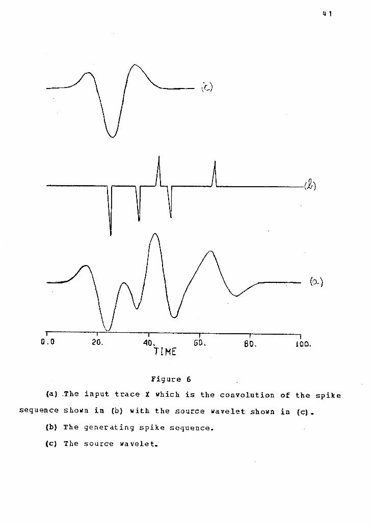
The i n p u t t r a c e X s h o w n i n F i g u r e 6 (a) i s a r e s u l t o f t h e

c o n v o l u t i o n o f t h e w a v e l e t s h o w n i n F i g u r e 6 (c) a n d t h e s p i k e

s e g u e n c e o f F i g u r e 6 ( b ) . T h i s t r a c e h a s b e e n c o n v o l v e d w i t h t h e

MED f i l t e r a n d t h e r e s u l t a n t s p i k e t r a c e Y° i s s h o w n i n F i g u r e

7. T h e s p i k e t r a c e Y° was t r u n c a t e d f r o m b o t h s i d e s s o t h a t

i t s l e n g t h w i l l f o l l o w t h e r e l a t i o n " l e n g t h o f o b s e r v a t i o n s =

l e n g t h o f s p i k e s e q u e n c e + l e n q t h o f w a v e l e t - 1" a n d t h e

r e s u l t a n t t r a c e i s t h e s p i k e s e q u e n c e Y c h o s e n a s t h e p a r t o f

t h e t r a c e b e t w e e n t h e a r r o w s i n F i g u r e 7. T r u n c a t i o n i s b a s e d

on i n t e r p r e t a t i o n o f t h e n u m e r i c a l v a l u e s o f t h e t r a c e Y ° . I n

t h i s e x a m p l e i t i s c l e a r w h e r e Y° s h o u l d be t r u n c a t e d , s i n c e

i t i s d e s i r a b l e t h a t t h e s p i k e s i g n a l i n c l u d e s t h e l a r g e r s p i k e s

o f t h e MED o u t p u t . N o t e t h a t Y ( t h e t r u n c a t e d t r a c e ) i n c l u d e s

o n l y t h e s e c t i o n o f Y ° t h a t c o n t a i n s t h e m a j o r s p i k e s . T h a t

i s , t h e i n t e r p r e t a t i o n h a s a s s u m e d t h a t s m a l l a m p l i t u d e ' b u m p s '

a r e n o i s e a n d c a n b e r e j e c t e d .

U s i n g t h e i n v e r s i o n s c h e m e s d e s c r i b e d p r e v i o u s l y , w i t h t h e

i n p u t X a n d Y a s s p e c i f i e d a b o v e , we g e t t h e r e s u l t s s h o w n

i n F i g u r e 8. T h e i n v e r s e o p e r a t o r o f t h e MED f i l t e r ( F i g u r e

TIME

F i g u r e 6 (a) The i n p u t t r a c e X which i s the c o n v o l u t i o n o f the s p i k e

seguence shown i n (b) with the source wavelet shown i n ( c ) .

(b) The g e n e r a t i n g s p i k e sequence.

(c) The source wavelet.

H2

r

o. 2D. AQ. TIKE

eo. 80. 1 0 0 .

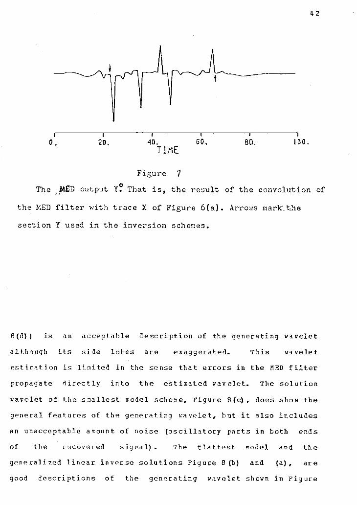
F i g u r e 7

The MED o u t p u t Y? That i s , t h e r e s u l t o f t h e c o n v o l u t i o n of

t h e MED f i l t e r w i t h t r a c e X o f F i g u r e 6 ( a ) . Arrows mark", t h e

s e c t i o n Y used i n t h e i n v e r s i o n schemes.

fl(d)) i s an acceptable d e s c r i p t i o n of the generating wavelet although i t s s i d e lobes are exaggerated. T h i s wavelet e s t i m a t i o n i s l i m i t e d i n the sense that e r r o r s i n the MED f i l t e r propagate d i r e c t l y i n t o the estimated wavelet. The s o l u t i o n wavelet of the s m a l l e s t model scheme. Figure 0 ( c ) , does show the general f e a t u r e s of the generating wavelet, but i t a l s o i n c l u d e s an unacceptable amount of noise ( o s c i l l a t o r y parts i n both ends of the recovered s i g n a l ) . The f l a t t e s t model and the g e n e r a l i z e d l i n e a r i n v e r s e s o l u t i o n s F i g u r e 8(b) and (a), are good d e s c r i p t i o n s of the g e n e r a t i n g wavelet shown i n F i g u r e

43

6(c).

Except for p o l a r i t y reversals, which r e s u l t from p o l a r i t y

reversal of the MED output, the estimated wavelets shown i n

Figure 8 are acceptable descriptions of the source wavelet.

However, the correct amplitude r e l a t i o n of the small lobes which

precede and follow the large amplitude part of the s i g n a l has

been l o s t . The deviation of the estimated wavelets from the

generating wavelet i s a r e s u l t of the small numerical noise that

contaminates the estimated spike sequence (the MED output) . As

mentioned i n the section P r a c t i c a l Notes, paragraph (e), we

expect to get the best results when Q1 and N1 assume the

value 5 9 , the assumed length of the wavelet. The generalized

li n e a r inverse model (Figure 8 ( a ) ) , and the f l a t t e s t model

(Figure 8 ( b ) ) , behaved i n t h i s manner but the smallest model

(Figure 8(c)) did not. I t i s possible that either the smallest

model scheme i s more sensitive to noise or that the box car

representation of the kernels i s inadequate, or both.

The spike trace can be treated further by setting

Yi 0 . 1

(32) Yj = 0 lyj < o.i

This s p e c i f i c a t i o n i s j u s t i f i e d by the assumption that the small

values i n the MED output are actually ncise which has been

generated by the MED algorithm. The v a l i d i t y of t h i s assumption

can be checked by synthetic examples. Comparison of Figure 6(b)

r 1 1 1 r 0.0 20. 40, 60. gO.

T I M E

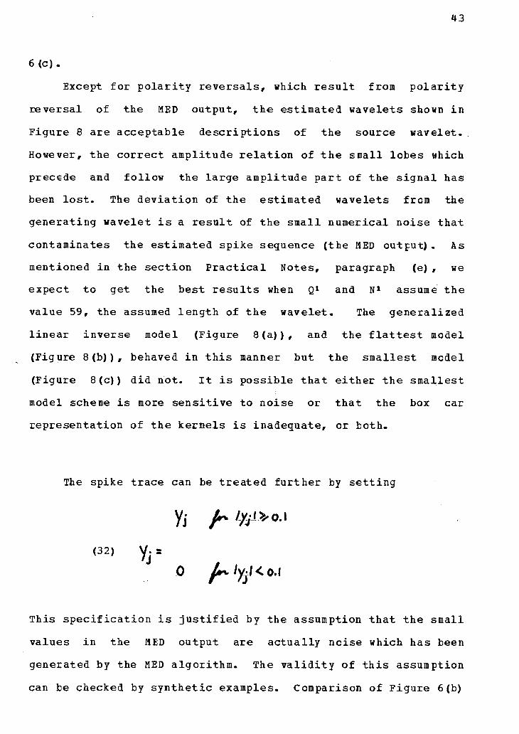
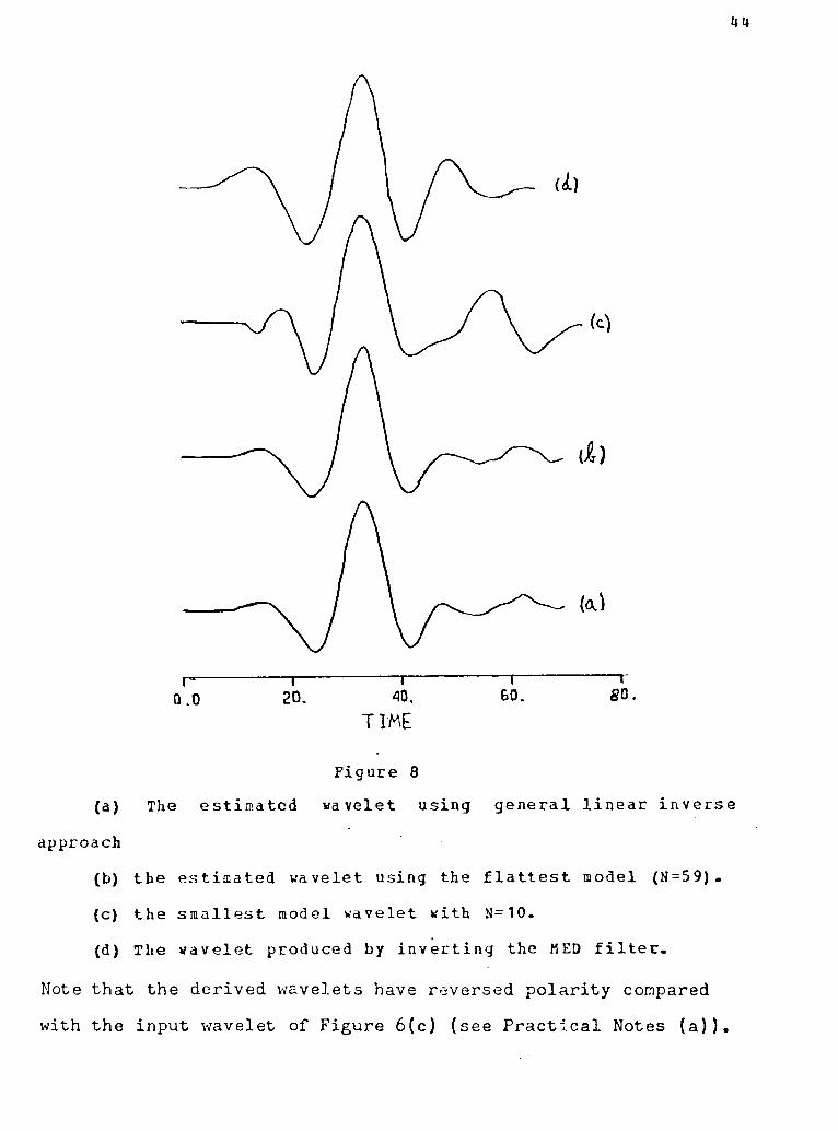
F i g u r e 8

(a) The estimated wavelet using general l i n e a r inverse

approach (b) the estimated wavelet using the f l a t t e s t model ( N = 5 9 ) . (c) the smallest model wavelet with N=10.

(d) The wavelet produced by i n v e r t i n g the MED f i l t e r -

Note that the derived wavelets have reversed p o l a r i t y compared

with the input wavelet of Figure 6(c) (see P r a c t i c a l Notes ( a ) ) .

45

with Figure 7 shows that the MED output does include some small

•bumps' which were not included i n the generating spike

sequence. Equation (32) excludes those 'bumps' from the input

spike sequence Y.

The spike trace Y as defined i n equation (32) and trace

X of Figure 6(a) are processed with the inversion procedures.

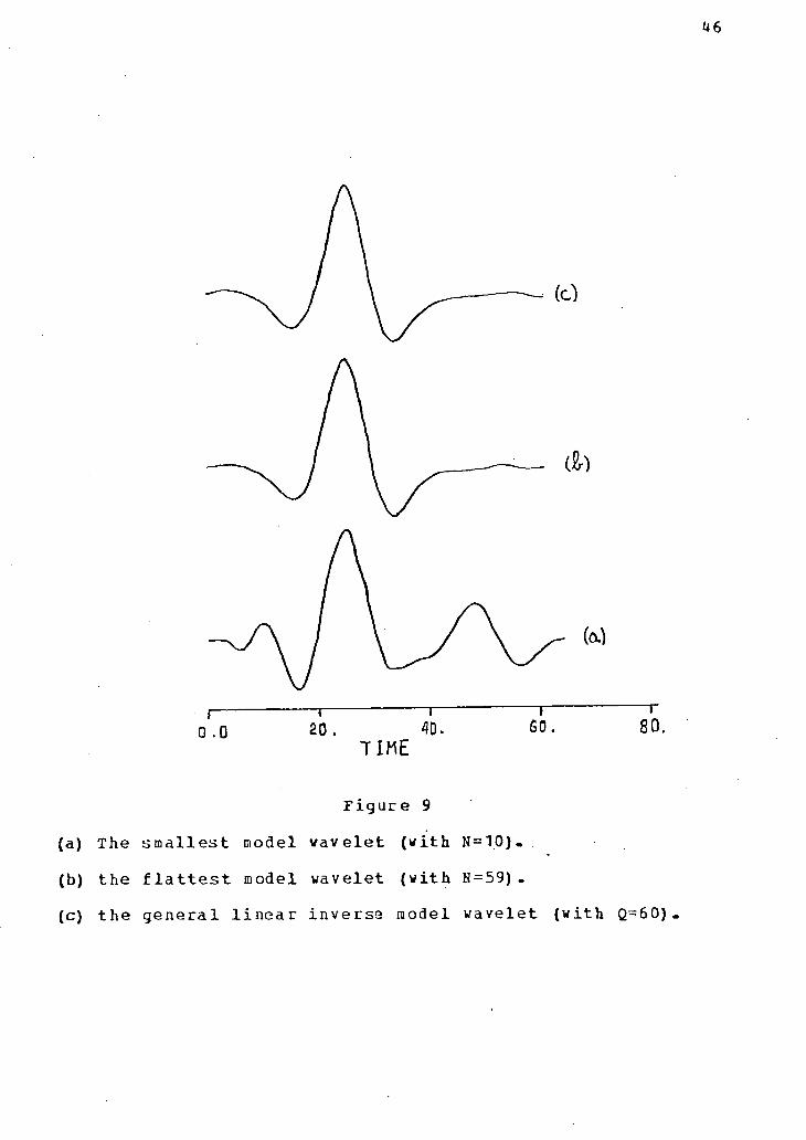
The results are shown i n Figure 9. The smallest model wavelet

Figure 9(a) does not reproduce the source wavelet to within the

expected standard. For t h i s reason, we w i l l not show ad d i t i o n a l

examples using the smallest model calcu l a t i o n s . Note that the

models of Figure 9(b) and (c) reproduce the o r i g i n a l wavelet

very well.

The exact reproduction of the input wavelet by the f l a t t e s t

model (Figure 9(b)), and the generalized l i n e a r inverse model

(Figure 9 (c)), i s expected, since i n t h i s p a r t i c u l a r example

eguation (32) converts the problem to an almost noiseless one.

i \ 1 J r

0 . 0 2 0 . 40. SO. 8 0 . T I M E

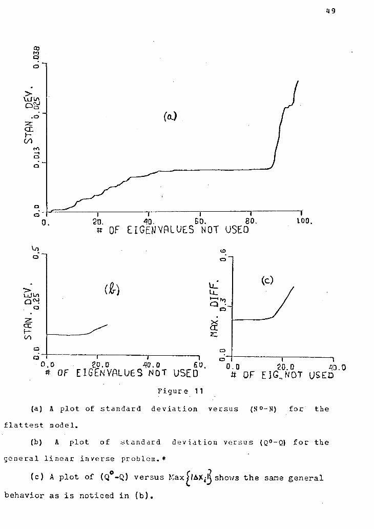
F i g u r e 9

(a) The smallest model wavelet (with N=10).

(b) the f l a t t e s t model wavelet (with N=59).

(c) the general l i n e a r inverse model wavelet (with Q=60).

47

Example B (Low q u a l i t y MED output)

This example was designed to demonstrate the performance of

the different approaches i n cases of low q u a l i t y spike traces.

We w i l l show that the l i n e a r inversion schemes are capable of

extracting useful information out of seemingly meaningless spike

traces.

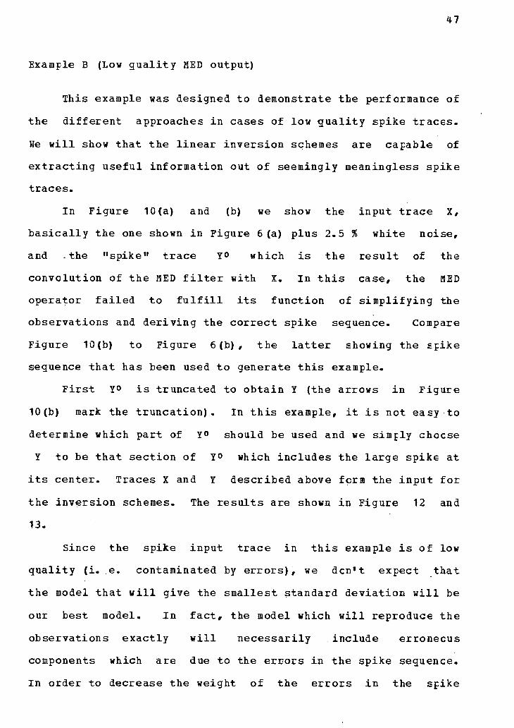
In Figure 10(a) and (b) we show the input trace X,

b a s i c a l l y the one shown in Figure 6(a) plus 2.5 % white noise,

and -the "spike" trace Y<> which i s the re s u l t of the

convolution of the MED f i l t e r with X. In t h i s case, the MED

operator f a i l e d to f u l f i l l i t s function of simplifying the

observations and deriving the correct spike sequence. Compare

Figure 10(b) to Figure 6(b), the l a t t e r showing the spike

sequence that has been used to generate t h i s example.

F i r s t Y° i s truncated to obtain Y (the arrows i n Figure

10(b) mark the truncation). In t h i s example, i t i s not easy to

determine which part of Y° should be used and we simply cheese

Y to be that section of Y° which includes the large spike at

i t s center. Traces X and Y described above form the input for

the inversion schemes. The results are shown i n Figure 12 and

13.

Since the spike input trace i n t h i s example i s of low

guality ( i . e. contaminated by errors), we den't expect that

the model that w i l l give the smallest standard deviation w i l l be

our best model. In f a c t , the model which w i l l reproduce the

observations exactly w i l l necessarily include erroneous

components which are due to the errors in the spike sequence.

In order to decrease the weight of the errors i n the spike

HQ

I 1 1 J 1 1

0. 20. 40. 60. 80. 100.

TIME

F i g u r e 10 (a) The input trace X of example B. This trace i s

b a s i c a l l y the one shown i n Figure 6(a) plus 2.5% white noise. o

(b) The M ED output Y used in example B. This trace i s the

convolution of the tr a c e i n (a) and tne MED f i l t e r . Arrows mark,

the section used i n the i n v e r s i o n .

49

Co a o

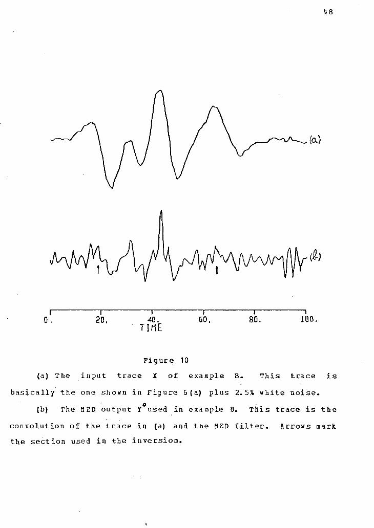
Figure 11

(a) A p l o t o f s t a n d a r d d e v i a t i o n v e r s u s (N°-N) f o r t h e

f l a t t e s t n o d e l .

(b) A p l o t o f s t a n d a r d d e v i a t i o n v e r s u s (Q°-Q) f o r t h e

g e n e r a l l i n e a r i n v e r s e p r o b l e m . *

(c) A p l o t of (Q°-Q) v e r s u s Max £lAX,-lj shows t h e same g e n e r a l

b e h a v i o r as i s n o t i c e d i n ( b ) .

50

sequence we have to allow some 'errors' i n the reproduced

observations. Hence we w i l l have to use the.plots of standard

deviation, and maximum error, in order to analyse the d i f f e r e n t

possible models (see section P r a c t i c a l Notes, paragraph (c)).

In Figure 11(a), the standard deviation for the f l a t t e s t model

versus (N°-N) i s plotted. In t h i s example N1 (practical rank

of P ) i s 55. Note the f l a t region corresponding to 45<N°-

N<90. The significance of t h i s region i s that a l l models i n

which 10<N<55 reproduce the observations to within the same

standard deviation and hence they can be represented by two

models, one for each end of t h i s region.

A plot of the standard deviation and the maximum error

versus Q°-Q (Figures 11(b) and (c)) for the generalized l i n e a r

inverse model shows a f l a t region corresponding to Q°-Q<16.

Here we w i l l represent a l l those models i n which 40<Q<56 by cne

model, corresponding to the center of t h i s f l a t region.

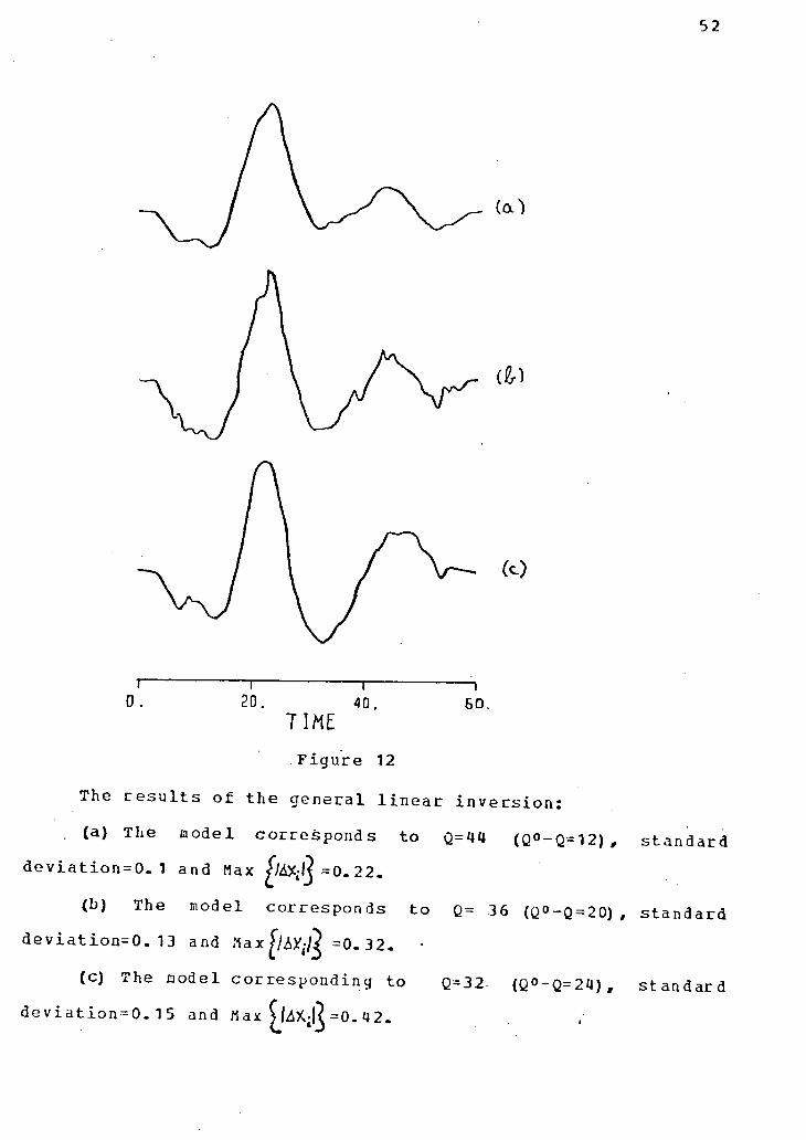
The solution wavelets that represent the d i f f e r e n t groups

are shown in Figure 12 f o r the generalized l i n e a r inverse and

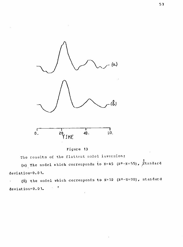
Figure 13 for the f l a t t e s t model solutions. Note the s i m i l a r i t y

i n the general features of the d i f f e r e n t models. The f l a t t e s t

model solution corresponding to N=10 (Figure 13(b)) i s the best

estimated wavelet. This i s an excellent estimation considering

the quality of the input spike sequence. Compare Fiqures 13 (b)

and 6 (c), and consider the fact that we used the spike sequence

shown in Figure 10(b) which poorly resembles the true spike

seguence of Figure 6(b).

Note that the large amplitude part of the signal does not

change much from one model to another. This type of behavior

51

has been discussed in the P r a c t i c a l Notes, paragraph (c).

Example C (Synthetic seismogram)

In the following example we w i l l show that the assumption

that a seismogram can be modelled as the convolution of a

wavelet with the earth's response where the response function i s

represented by the MED output, i s useable. This assumption

enables a representative wavelet to be computed.

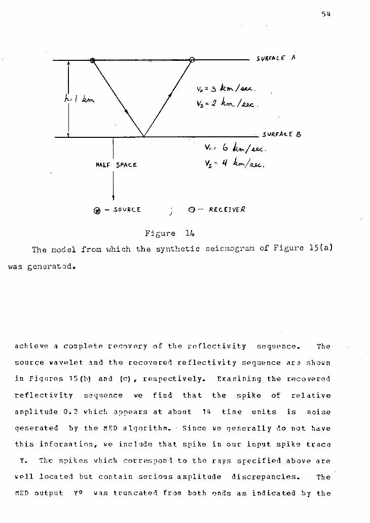
A synthetic seismogram using generalized ray theory

(Wiggins and Helmberger 1974) has been computed from the model

shown i n Figure 14. The following rays were considered :

1. Leaving the source as a P wave and received as a P

wave ; a r r i v a l time 0.745 sec; r e l a t i v e amplitude 0.33.

2. Leaving the source as P and received as S ; a r r i v a l

time 0.928 sec for the reflected energy and 0.927 sec for the

refracted energy; r e l a t i v e amplitude for the combined response

i s 0..385.

3. Leaving the source as a S wave and received as S ;

a r r i v a l time 1.119 sec; r e l a t i v e amplitude 1.0.

4. Leaving the source as P, r e f l e c t i n g frcm surface B,

r e f l e c t i n g from surface A, bouncing again frcm surface B and

received as P ; a r r i v a l time 1.374 sec; r e l a t i v e amplitude 0.09.

Figure 15(a) shows the synthetic trace computed from these

ray paths. The model was constructed such that i t w i l l show

strong interference. In such a case, the MED algorithm cannot

52

(£•)

r 0 .

T r 20. 40,

TIME B O .

F i g u r e 12

The r e s u l t s o f t h e g e n e r a l l i n e a r i n v e r s i o n :

(a) The model c o r r e s p o n d s t o Q=4«J (Q°-Q=12), s t a n d a r d d e v i a t i o n s . 1 and Max =0. 22.

(b) The model c o r r e s p o n d s t o Q= 36 (Q°-Q=20), s t a n d a r d

d e v i a t i o n = 0 . 13 and ,1ax ̂ /iX,/^ =0. 32.

(c) The model c o r r e s p o n d i n g t o Q=32 (Q°-Q=24), s t a n d a r d

d e v i a t i o n s . 1 5 and Max ^J4X;|^ =0. 42.

53

I 1 1 1 0. 80. 40. 50.

T I M E

F i g u r e 13

The r e s u l t s of t h e f l a t t e s t n o d e l i n v e r s i o n : s

(a) The model which corresponds to N=45 ( N ° - N = 5 5 ) , Standard deviatiou=0. 0 1.

(bv) -the model which corresponds to N=10 ( N ° - N = 9 0 ) # standard deviation=0. 0 1. '

54

H A L F S P A C E

- SOURCE

SURFACE 6

O— RECEIVE/?

Figure 14

The model from which the synthetic seismogram of Figure 15(a)

was generated.

a c h i e v e a c o n p l e t e r e c o v e r y o f t h e r e f l e c t i v i t y s e q u e n c e . The

s o u r c e v a v e l e t and t h e r e c o v e r e d r e f l e c t i v i t y s e q u e n c e a r e shown

i n F i g u r e s 15(b) and (c) , r e s p e c t i v e l y . E x a m i n i n g t h e r e c o v e r e d

r e f l e c t i v i t y s e q u e n c e we f i n d t h a t t h e s p i k e o f r e l a t i v e

a m p l i t u d e 0.2 w h i c h a p p e a r s a t a b o u t 14 t i m e u n i t s i s n o i s e

g e n e r a t e d by t h e MED a l g o r i t h m . S i n c e ve g e n e r a l l y do n o t h a v e

t h i s i n f o r m a t i o n , we i n c l u d e t h a t s p i k e i n o u r i n p u t s p i k e t r a c e

Y. The s p i k e s w h i c h c o r r e s p o n d t o t h e r a y s s p e c i f i e d a b o v e a r e

w e l l l o c a t e d b u t c o n t a i n s e r i o u s a m p l i t u d e d i s c r e p a n c i e s . The

MED o u t p u t Y° was t r u n c a t e d from b o t h ends a s i n d i c a t e d by t h e

5 5

(I)

0. ~T r~ 20. 40.

T I M E

(c)

60,

T 1 1 > 0 . 0 . 7 lA 2.1

S E C .

Figure 15

(a) The input trace X which i s the synthetic seismogram of the model i n Figure 1/+.̂ ( b ) The source wavelet. ( c ) The MED output, the trace Y, which i s the r e s u l t of the convolution of the MED f i l t e r with X. Arrows mark the section used i n the i n v e r s i o n .

56

arrows in Figure 15(c). The resultant spike trace Y and the

input trace X (Figure 15(a)) served as input to the l i n e a r

inversion schemes.

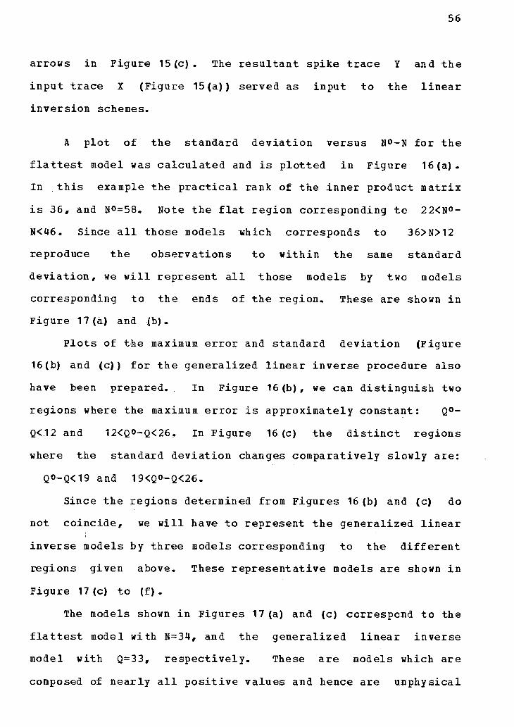
A plot of the standard deviation versus N°-N for the

f l a t t e s t model was calculated and i s plotted i n Figure 16(a).

In t h i s example the p r a c t i c a l rank of the inner product matrix

i s 36, and N°=58. Note the f l a t region corresponding t c 22<N°-

N<46. Since a l l those models which corresponds to 36>N>12

reproduce the observations to within the same standard

deviation, we w i l l represent a l l those models by two models

corresponding to the ends of the region. These are shown i n

Figure 17(a) and (b).

Plots of the maximum error and standard deviation (Figure

16(b) and (c)) for the generalized l i n e a r inverse procedure also

have been prepared.. In Figure 16(b), we can distinguish two

regions where the maximum error i s approximately constant: Q°-

Q<12 and 12<0_o-Q<26. In Figure 16 (c) the d i s t i n c t regions

where the standard deviation changes comparatively slowly are:

Q0-Q<19 and 19<Q0-Q<26.

Since the regions determined from Figures 16(b) and (c) do

not coincide, we w i l l have to represent the generalized l i n e a r

inverse models by three models corresponding to the di f f e r e n t

regions given above. These representative models are shown i n

Figure 17(c) to ( f ) .

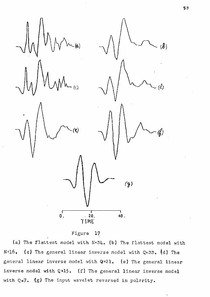
The models shown i n Figures 17(a) and (c) correspond to the

f l a t t e s t model with N=34, and the generalized l i n e a r inverse

model with Q=33, respectively. These are models which are

composed of nearly a l l positive values and hence are unphysical

S7

o

. a

CO

o

a ( a )

0. ?0. 40. GO. tf OF EIGENVALUES NOT USED

o

a • j o

cr.

0. 20. 40. » QF EIGENVALUES NOT USED

a a

t

0. , 20. 40. * OF E I G E N V A L U E S NOT U S E D

F i g u r e 1 6

(a) A p l o t of N°-N versus standard deviation f o r

the f l a t t e s t model.

(b) A p l o t of Q° - Q versus Hax^/AV-/^, f o r the

general l i n e a r inverse.

(c) A p l o t of Q°-Q versus standard deviation , for the

general l i n e a r inverse.

58

TIKE

F i g u r e 17

(a) The f l a t t e s t model with N=34. (b) The f l a t t e s t model with

N-16. (c) The general l i n e a r inverse model with Q-33. (d) The

general l i n e a r inverse model wdth Q=21. (e) The general l i n e a r

inverse raodel with Q*15. (f) The general l i n e a r inverse model

with Q^7. (g) The input wavelet reversed i n p o l a r i t y .

59

because we expect the wavelet to include positive and negative

values. That i s , we expect tensional stresses to fellow

compressional stresses or positive displacements to be followed

by negative ones. Therefore these models are abandoned on

physical grounds.

The remaining model wavelets shown i n Figure 17 describe

the source wavelet of Figure 15(b) with varying degrees of

accuracy. A l l of these models provide a consistent description

of the general features of the source wavelet i n the region 7 to

21 time units. However the wavelet of (e) which i s the general

l i n e a r inverse model with Q=15 and the wavelet of (f)

corresponds to the drop i n Max£|4Xi|^ i n Figure 16(b) (Q=7) ,

represent the true wavelet more closely and either could be

chosen as an appropriate representation.

CONCLUSION

In t h i s chapter we have shown that the l i n e a r inversion

schemes are capable of extracting a great deal of information

from a wide variety of input data. We concentrated p a r t i c u l a r l y

on seemingly unreliable data since that i s where we could show

the f u l l power of the l i n e a r inverse technigues.

The smallest model inversion has proved i n f e r i o r for t h i s

p articular problem, probably because we represented the spike

sequence Y as a series of box cars.

The f l a t t e s t model approach performed s l i g h t l y better on

example B, while the general l i n e a r inverse scheme gave somewhat

60

better r e s u l t s i n example C. Both techniques determined the

main features of the input wavelet (in the case of example C,

the region between time units 10 to 20 i n the solution models).

Since two integrations are involved i n the Backus-Gilbert

f l a t t e s t model c a l c u l a t i o n , we expect that the error w i l l be

smoothed out. This w i l l happen only i f the spike input Y i s a

"high freguency" trace ; i n other words only i f the wavelet

length i s large compared to the dominant period i n the spike

trace. I t i s probable that the f l a t t e s t model didn't perform as

well i n example C, because of the predominant lew frequency of

the spike trace Y of that example. Past experience with MED

output shows that, in general, we can expect the dominant period

i n the MED output to be small compared to the wavelet length.

Hence we can expect substantial smoothing of the error i n the

f l a t t e s t model scheme.

Since the generalized l i n e a r inverse i s a parametric

approach i t does not require continuous representation for the

MED output. Also i t does not involve integrations and hence

seems to be computationaly simpler. However, the method

reguires decomposition of an nXm matrix which needs more

computer time then the square matrix decomposition reguired by

the Backus-Gilbert approach. For Q equal to the p r a c t i c a l rank

of A and N equal to the p r a c t i c a l rank of /"* , the models

generated by the generalized l i n e a r inverse and f l a t t e s t model

are almost i d e n t i c a l .

We demonstrated the importance of the plots of maximum

error and standard deviation versus the number of eigenvalues

not used in the solution , and showed how such plots can be used

61

to reduce the p r a c t i c a l number of models. At t h i s time, i t i s

not possible to suggest an a n a l y t i c a l way to enable the user to

choose the best model out of the given group's representative

set. The user w i l l have to t r y each group's representative

model as a possible estimated wavelet.

However, one might get some i n d i c a t i o n on the quality of

the estimated wavelet, by formulating a new l i n e a r inverse

problem of the form:

x=w**s

where * denotes convolution and

X i s the observation vector, — Ok. Wl i s the • estimated wavelet vector, and _ • . * i

S* i s the . ( recovered spike sequence.

Then one solves for the spike sequence SA. Having the set

of spike sequences S 1 one calculates the associated set of

varimaxes V . The "best" estimated wavelet i s the one which i s «

associated with the highest varimax trace S*.

62

CHAPTEB 4

Debubblinq as a Generalized Linear Inverse Problem

INTRODUCTION

The bubble pulse problem i s common to many marine energy

sources and has been discussed in d e t a i l by Kramer et a l (1S68).

The problem i s caused by successive o s c i l l a t i o n s of the gas

bubble generated by the energy source. Each cycle of the

o s c i l l a t i n g bubble corresponds to a signal propagating outward.

The source wavelet as recorded on a seismic trace i s then a

t r a i n of the wavelets generated by the i n d i v i d u a l cycles. The

number of pulses and the i r periods are primarily a function of

detonation depth and energy released during creation of the

bubble. The length of the compound wavelet depends on the

number of expand-collapse cycles of substantial energy generated

by the bubble, u n t i l i t has completely collapsed inward or

vented remaining energy to the atmosphere. Duration of the

compound wavelet often exceeds 0.5 sec. . This excesive length

creates severe interference problems and causes masking of

events, e s p e c i a l l y on those parts of seismograms following large

amplitude r e f l e c t i o n s .

The aim of debubbling schemes i s to eliminate the bubble

puls€ e f f e c t s , and to compress the compound wavelet signature to

one that i s simple and of short duration. Mateker ( 1 9 7 1 )

suggested a debubbling scheme which shapes the recorded source

63

wavelet into a pulse at the time of the i n i t i a l pulse. This

process can be ca r r i e d out through the use of the Weiner shaping

f i l t e r s . Recently, Wood et a l (1978) suggested two clos e l y

related methods. The f i r s t can be described by the following

stages :

1. Crosscorrelate the data and the known source

signature. The resultant trace has a better signal tc noise

r a t i o , and i t s wavelet i s the autocorrelation of the source

signature. The new wavelet i s a zero phase one.

2. Using Weiner f i l t e r s ( T r e i t e l and Robinson, 1 966),

shape the autocorrelated source wavelet i n t o a short duration

desired s i g n a l . When shaping the autocorrelated wavelet use the

fact that i t i s a zero phase wavelet, one of the advantages of

the crosscorrelation of step 1.

3. Apply the shaping f i l t e r of step 2 to the

crosscorrelated data.

The second i s s i m i l a r and can be described b r i e f l y as follows:

1. Crosscorrelation of the known source signature

with the data (as in step 1 above).

2. Compute the zero delay Weiner inverse f i l t e r of

the wavelet and apply i t to the data.

3. Crosscorrelate the zero delay Weiner inverse

f i l t e r of step 2 with the data.

As seen from the above discussion, currently used

debubbling methods employ Weiner shaping f i l t e r s i n their

algorithms. These depend c r i t i c a l l y on the choice of the length

of the f i l t e r (an unknown parameter), and cannot overcome

problems which a r i s e due to errors i n the recorded wavelet.

64

In t h i s work, a new and diff e r e n t approach to the

debubbling problem i s presented. I t makes use cf the

th e o r e t i c a l concepts embodied i n generalized l i n e a r inversion

(Wiggins et a l 1976; also see Chapter 3). This technigue i s

applied f i r s t to an estimation of the wavelet and secondly to

the debubbling of the seismic trace using the estimated wavelet.

Debubbling as a generalized l i n e a r inverse problem i s

described by the following steps, and shown schematically i n the

flow diagram of Figure 1.

1. Apply minimum entropy deconvolution (Wiggins 1977; also

see Chapter 2) to the observed data to get the deconvolved spike

trace.

2. Ose the deconvolved spike trace and the data as an

input to the generalized l i n e a r inverse procedure to compute the

estimated bubble pulse wavelet.

3. Use the information acquired i n steps 1 and 2 to

construct the compound source signature ( i . e . the i n i t i a l pulse

plus appropriate bubble o s c i l l a t i o n s ) .

4. Use the compound source signature and the observed data

as input to the generalized l i n e a r inverse scheme to determine

the estimated earth impulse response.

65

Figure 1

1. Data.

2. MED.

3. Deconvolved spike

t r a c e .

4 . Generalized l i n e a r

inverse.

5. Estimated wavelet.

6. Construction of the

compound signature.

7 . Debubbled trace Flow diagram of the proposed

debubbling procedure.

SOURCE S I A TUT? 7=: ESTIMATION AND DE3U3BLING

The assumption that a seismogram can be modelled as the convolution of the earth's impulse response with a source wavelet provides the b a s i s f o r t h i s work. Mathematically the statement i s

X=S*w • (1)

where 7. i s the observed seismogram, S i s the earth impulse response and W i s the source wavelet.

In summation n o t a t i o n equation (1) takes the form

66

AM

j=1 n, n i s the length of the observed data;

k=1.,. ...m, m i s the length of the wavelet; and

the r e l a t i o n n=l+m-1 must hold, where 1 i s the length

of the earth's impulse response.

Having the observed data (the seismogram) and either the

source signature or an estimate of the earth's response, one can

solve for the unknown time series. For the sake of the

discussion l e t us assume that we have the seismogram X and an

estimate of the source signature W. Writing eguation (2) i n i t s

matrix form we get :

X=A*S (3)

where

A( i , j) =W ( i - j + 1) j=1 1 ; i=1....n (4)

with

W(i-j + 1)=0 for i - j + 1<0 and i - j + 1>m

Eguation (3) represents an overdetermined system i n which

n>l, i . e. the number of eguations i s larger then the number t

of unknowns. We solve t h i s system of eguations by minimizing

the error vector AX=X° a s- X C A L i n a l e a s t squares sense. For

a more detailed discussion the reader i s referred to Chapter 3.

The least squares solution of (3) i s given by :

67

or i n summation notation

A..

where

0 T i s the transpose of U which consists of g eigenvectors

of length n associated with the columns of A; these vectors are

commonly referred to as the data eigenvectors.

V consists of g eigenvectors of length 1 associated with

the row vectors of A; these are commonly referred to as the

parameter eigenvectors.

A"' i s the inverse of A which consists of the q

eigenvalues of A in descending order. A = d i a g w h e r e q

i s the rank of A.

Equation (6) states that the desired earth response i s a

weighted summation of the parameter eigenvectors. It i s

advantageous to use equation (6) as our solution, p a r t i c u l a r i l y

when one i s dealing with noisy data or when the estimated source

signature i s contaminated by noise. In both cases one could

choose to r e j e c t the smaller and less r e l i a b l e eigenvalues

before proceeding with the c a l c u l a t i o n s (see Chapter 3). This

i s e a s i l y done by l e t t i n g Q i n equation (6) assume smaller and

smaller values. I t i s clear that the euclidian length of the

error vector AX grows as we reject more and more of the

smaller eigenvalues, but at the same time we eliminate the l e s s

(5)

(6)

68

r e l i a b l e components of the solution. A useful t o o l i n the

analysis of the d i f f e r e n t solutions (corresponding to d i f f e r e n t

Q values) i s the plot of the standard deviation (|4X|Z) versus

the number of eigenvalues rejected (see Chapter 3 ) .

In the alternative case where one has the seismogram X and

the estimated earth response S, the only change i n the above

eguations occurs i n the d e f i n i t i o n of A. Then A i s given by :

A ( i , j) =S ( i - j + 1) j = 1. m ; i = 1 n (7)

where

S(i-j+1)=0 for i-j+1<0 and i-j+1>l .

Eguations (5) and (6) s t i l l hold with W replacing S.

The flow diagram of Figure 1 outlines the procedure which

i s followed to obtain a debubbled seismic trace. Let us examine

the various steps.

Having the f i e l d trace, we aim f i r s t at an intermediate

target - estimation of the wavelet. To estimate the wavelet we

require a rough estimate of the earth's response. To f i n d that

estimate we apply MED to the data. This leads to step 1 i n the

computation procedure.

1. Apply minimum entropy deconvolution (Wiggins 1977 ;

also see Chapter 2) to the f i e l d data. The MED output serves as

a f i r s t approximation to the earth's impulse response.

A troublesome point i n step 1 concerns the choice of the

length of the MED f i l t e r . Long MED f i l t e r s tend to compress

much of the energy i n a trace into one large spike, t h i s

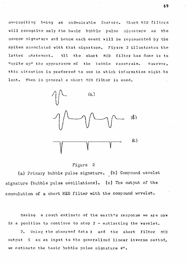
69

o v e r s p i k j. ng b e i n g an u n d e s i r a b l e f e a t u r e . S h o r t M E D f i l t e r s

w i l l r e c o g n i z e o n l y t h e b a s i c b u b b l e p u l s e s i g n a t u r e as t h e

s o u r c e s i g n a t u r e and h e n c e e a c h e v e n t w i l l be r e p r e s e n t e d by t h e

s p i k e s a s s o c i a t e d w i t h t h a t s i g n a t u r e . F i g •ire 2 i l l u s t r a t e s t h e

l a t t e r s t a t e m e n t . M l t h e s h o r t MED f i l t e r h as done i s t o

" s p i k e up" t h e a p p e a r a n c e o f the b u b b l e w a v e t r a i n . However,

t h i s s i t u a t i o n i s p r e f e r r e d t o one i n which i n f o r m a t i o n m i g h t be

l o s t . Then i n g e n e r a l a s h o r t M E D f i l t e r i s u s e d .

Figure 2

(a) Primary bubble pulse signature. (b) Compound wavelet

signature (bubble pulse o s c i l l a t i o n s ) . (c) The output of the

convolution of a short MED f i l t e r with the compound wavelet.

H a v i n g a r o u g h e s t i m a t e o f t h e e a r t h ' s r e s p o n s e we a r e now

i n a p o s i t i o n t o c o n t i n u e t o s t e p 2 - e s t i m a t i n g t h e w a v e l e t .

2. U s i n g t h e o b s e r v e d d a t a X and t h e s h o r t f i l t e r MED

o u t p u t 5 a s an i n p u t t o t h e g e n e r a l i z e d l i n e a r i n v e r s e method,

we e s t i m a t e t h e b a s i c b u b b l e p u l s e s i g n a t u r e W .

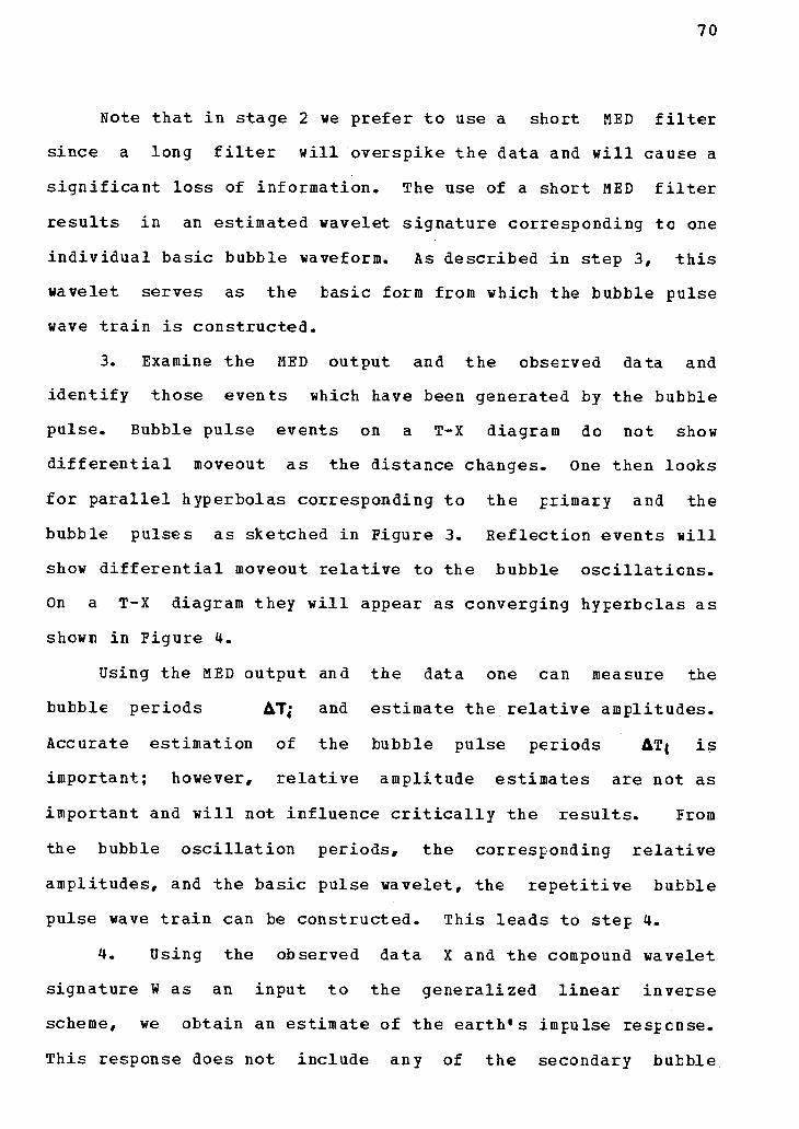
70

Note that i n stage 2 we prefer to use a short MED f i l t e r

since a long f i l t e r w i l l overspike the data and w i l l cause a

s i g n i f i c a n t loss of information. The use of a short MED f i l t e r

r e s u l t s i n an estimated wavelet signature corresponding to one

in d i v i d u a l basic bubble waveform. As described i n step 3, t h i s

wavelet serves as the basic form from which the bubble pulse

wave t r a i n i s constructed.

3. Examine the MED output and the observed data and

ide n t i f y those events which have been generated by the bubble

pulse. Bubble pulse events on a T-X diagram do not show

d i f f e r e n t i a l moveout as the distance changes- One then looks

for p a r a l l e l hyperbolas corresponding to the primary and the

bubble pulses as sketched in Figure 3. Reflection events w i l l

show d i f f e r e n t i a l moveout re l a t i v e to the bubble o s c i l l a t i o n s .

On a T-X diagram they w i l l appear as converging hyperbolas as

shown in Figure 4.

Using the MED output and the data one can measure the

bubble periods A T ; and estimate the r e l a t i v e amplitudes.

Accurate estimation of the bubble pulse periods ATj i s

important; however, r e l a t i v e amplitude estimates are not as

important and w i l l not influence c r i t i c a l l y the re s u l t s . From

the bubble o s c i l l a t i o n periods, the corresponding r e l a t i v e

amplitudes, and the basic pulse wavelet, the r e p e t i t i v e bubble

pulse wave t r a i n can be constructed. This leads to step 4.

4. Using the observed data X and the compound wavelet

signature W as an input to the generalized l i n e a r inverse

scheme, we obtain an estimate of the earth's impulse response.

This response does not include any of the secondary bubble

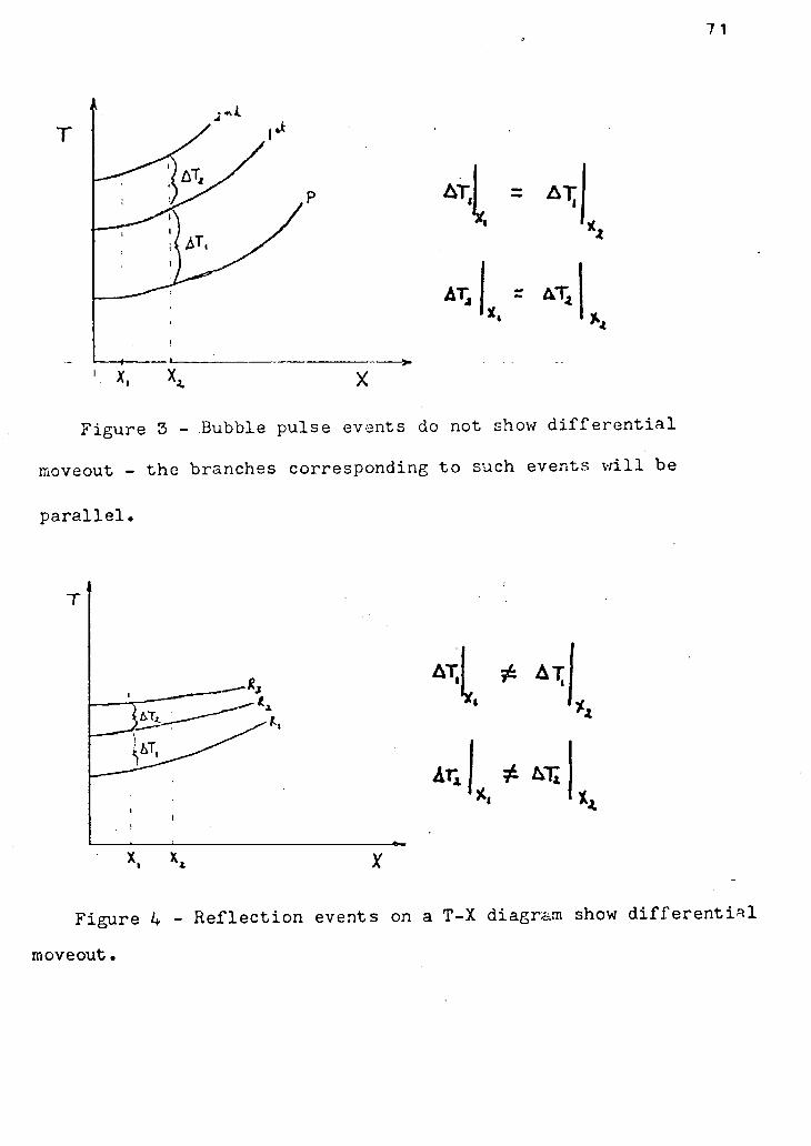
7 1

. . I , . ^ ' X, X, x

Figure 3 - Bubble pulse events do not show d i f f e r e n t i a l

moveout - the branches corresponding to such events w i l l be

p a r a l l e l .

T

Figure 4 - R e f l e c t i o n events on a T-X diagram show d i f f e r e n t i a l

moveout.

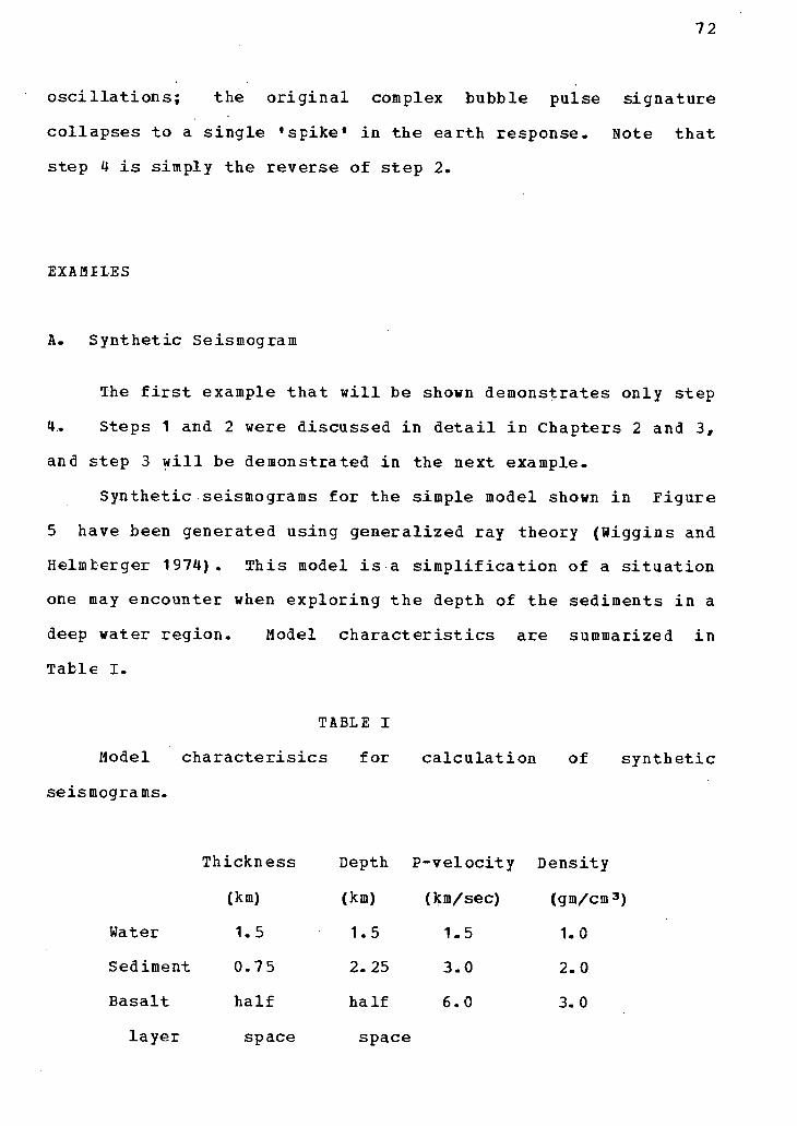
72

o s c i l l a t i o n s ; the o r i g i n a l complex bubble pulse signature

collapses to a single 'spike 1 i n the earth response. Note that

step 4 i s simply the reverse of step 2.

EXAME1ES

A. Synthetic Seismogram

The f i r s t example that w i l l be shown demonstrates only step

4,. Steps 1 and 2 were discussed i n d e t a i l i n Chapters 2 and 3,

and step 3 w i l l be demonstrated i n the next example.

Synthetic seismograms for the simple model shown i n Figure

5 have been generated using generalized ray theory (Wiggins and

Helmterger 1974). This model i s a s i m p l i f i c a t i o n of a s i t u a t i o n

one may encounter when exploring the depth of the sediments i n a

deep water region. Model c h a r a c t e r i s t i c s are summarized i n

Table I.

TABLE I

Model ch a r a c t e r i s i c s for c a l c u l a t i o n of synthetic

seismograms.

Thickness Depth P -vel o c i t y Density

(km) (km) (km/sec) (gm/cm3)

Water 1.5 1.5 1.5 1. 0

Sediment 0.75 2. 25 3.0 2.0

Basalt half half 6.0 3. Q

layer space space

73

In t h i s example, the primary P r e f l e c t i o n s with

v e r t i c a l t r a v e l times of 2 sec for the sea bottom r e f l e c t i o n and

2.5 sec for the r e f l e c t i o n from the base of the sediments w i l l

be considered. The compound wavelet which has been used (Figure

6) was constructed to simulate an energy source which sends out

a primary signal followed by two bubble pulses. Relative

amplitudes and the corresponding bubble periods are shown i n

Figure 6. Total length of the compound wavelet i s 0^6 sec.

These wavelet c h a r a c t e r i s t i c s were chosen because of the

s i m i l a r i t y with the expected c h a r a c t e r i s t i c s of the f i e l d

example to be described next.

Eight synthetic traces were generated corresponding to

offsets between 0.2 km and 1.6 km with receiver separation of

0.2 km. The traces were normalized such that the largest

amplitude i n each trace was unity (Figure 7 ) . Relative

amplitudes for r e f l e c t i o n s from the base of the sediments range

from 0.22 for the near v e r t i c a l r e f l e c t i o n s to 0.1 f o r the

widest angle r e f l e c t i o n s . Numerical noise l e v e l i n the

synthetic seismograms increases with the o f f s e t as a re s u l t of

longer c a l c u l a t i o n i n t e r v a l s . Note that the type cf behavior

shown i n Figures 3 and 4 i s c l e a r l y observed i n t h i s synthetic

example. In p a r t i c u l a r , the r e f l e c t i o n from the base of the

sediments i s hidden by the bubble pulse events on traces 1 to 4

while i t can be observed from traces 5 to 8.

The synthetic seismograms of Figure 7 and the bubble

o s c i l l a t i o n wavelet of Figure 6 formed the input to the

generalized l i n e a r inverse scheme as discussed i n step 4. The

debubbled seismograms determined from application of the inverse

7 4

water

sediments

b a s a l t i c l a y e r

\.G KM

O . U « - * | | < -

X O B — - Q & 1 - O - 0 "

I. V " / c c

£ _ .2 .0 ^ V c c

-SA^r-^ace

sea f l o o r

Figure 5 - The l a y e r model used in the construction of the

synthetic seisnogram.

Figure 6 - Signature of the compound source wavelet used t o

generate the synthetic seismogram.

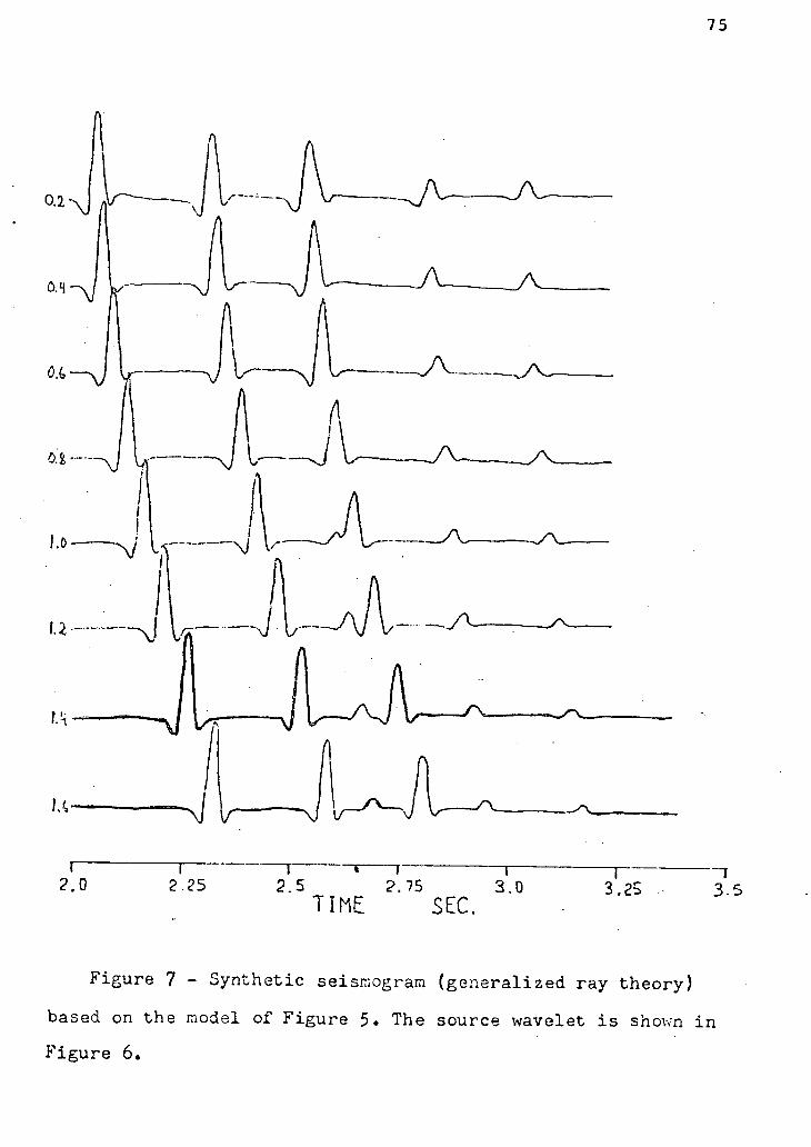
Figure 7 - Synthetic seismogram (generalized ray theory)

based on the model of Figure 5. The source wavelet i s shown i n

Figure 6.

76

procedure to each trace i s shown in Figure 8. Two major e f f e c t s

are noted. F i r s t , the extended bubble pulse o s c i l l a t i o n wave

tr a i n has been reduced to just one pulse, and further t h i s pulse

has been compressed to have a greater ' s p i k e - l i k e 1 character.

Also, as the numerical noise l e v e l increases, the solution

becomes more o s c i l l a t o r y as evidenced by traces 7 and 8. On

these traces, the r e f l e c t i o n from the base of the sediments

shows only marginally above the background noise l e v e l .

Considering that the r a t i o of the smaller amplitude

r e f l e c t i o n to the larger one i n traces 7 and 8 i s about one to

ten and that these traces include noise with a maximum amplitude

of about 50% of the smaller r e f l e c t i o n amplitude, the r e s u l t s of

Figure 8 form a good output.

B. FIELD EXAMPLE

Clowes et a l (1978) and Thorleifson (1978) have described a

marine deep seismic sounding program carried out i n Winona

Basin, a deep water (2 km) sedimentary basin located west of

northern Vancouver Island, B r i t i s h Columbia. Signals from six

i n d i v i d u a l hydrophones separated by 90m and suspended at 45m

depth from a 600m cable t r a i l e d behind the receiving ship were

recorded d i g i t a l l y while the shooting ship detonated explosive

charges ranging i n size from 2.2 kg to 200 kg at distances from

less then 1 to 95 km. Clowes (1977) has described the system i n

77

78

d e t a i l .

Seismograms from 2.2 kg shots were detonated at 7m and

recorded at distances up to about 6 km to form s u b - c r i t i c a l

incidence r e f l e c t i o n p r o f i l e s . Thorleifson (1978) has described

the interpretation of seme of these. Six traces from one shot

have been extracted from one p r o f i l e and are shown i n Figure 9.

For the purposes of t h i s study, these traces have been

normalized such that the maximum amplitude i n each trace has a

r e l a t i v e amplitude of 1.0. The data are bandpass f i l t e r e d from

5 to 3C hz.

The most prominent a r r i v a l s are the water bottom r e f l e c t i o n

with i t s associated bubble o s c i l l a t i o n s as indicated on the

figure by W, W1 and W2. By car e f u l l y looking at d i f f e r e n t i a l

moveout between d i f f e r e n t phases f o r many correlatable cycles,

Thorleifson (1978) was able to identi f y some primary r e f l e c t i o n s

from within the sediments of Winona Basin. His i d e n t i f i c a t i o n

of these events i s shown by the l e t t e r s A, B and C on Figure 9.

We note that the bubble pulse wave t r a i n shows the

ch a r a c t e r i s t i c s described i n Figure 3, while the primary

r e f l e c t i o n s show those depicted i n Figure 4.

From Figure 9, i t i s clear that the source wavelet with

bubble o s c i l l a t i o n s can be constructed from the primary pulse

followed by two bubble pulses. The f i r s t step i n our

debubbling-pulse compression procedure i s to estimate the basic

bubble pulse signature in every trace. We do not expect only

one basic bubble signature to hold for the d i f f e r e n t traces

since each of these corresponds to d i f f e r e n t angles of

incidence. The phase s h i f t problem might be circumvented by use

79

F i g u r e 9 - S i x t r a c e s from a r e f l e c t i o n p r o f i l e recorded o f f

Vancouver I s l a n d . Traces are at d i s t a n c e s from 1.0 to 1.5 km.

Each t r a c e i s n ormalized t o u n i t amplitude.

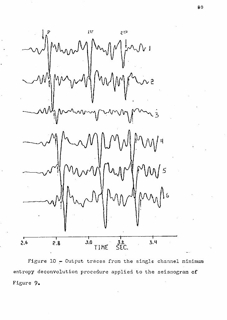
8 0

Figure 10 — Output traces from the single channel minimum

entropy deconvolution procedure applied to the seismogram of

Figure 9 .

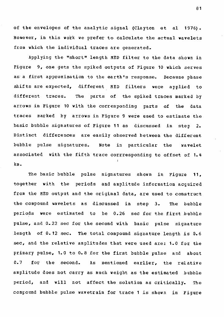
81

of the envelopes of the analytic s i g n a l (Clayton et a l 1976).

However, i n t h i s work we prefer to calculate the actual wavelets

from which the i n d i v i d u a l traces are generated.

Applying the "short" length MED f i l t e r to the data shown i n

Figure 9, one gets the spiked outputs of Figure 10 which serves

as a f i r s t approximation to the earth's response. Because phase

s h i f t s are expected, different MED f i l t e r s were applied to

dif f e r e n t traces. The parts of the spiked traces marked by

arrows i n Figure 10 with the corresponding parts of the data

traces marked by arrows i n Figure 9 were used to estimate the

basic bubble signatures of Figure 11 as discussed i n step 2.

Di s t i n c t differences are e a s i l y observed between the di f f e r e n t

bubble pulse signatures. Note i n p a r t i c u l a r the wavelet

associated with the f i f t h trace corrresponding to offset of 1.4

km.

The basic bubble pulse signatures shown i n Figure 11,

together with the periods and amplitude information acquired

from the MED output and the o r i g i n a l data, are used to construct

the compound wavelets as discussed i n step 3. The bubble

periods were estimated to be 0.26 sec for the f i r s t bubble

pulse, and 0.22 sec f o r the second with basic pulse signature

length of 0.12 sec. The t o t a l compound signature length i s 0.6

sec, and the r e l a t i v e amplitudes that were used are: 1.0 f o r the

primary pulse, 1.0 to 0.8 f o r the f i r s t bubble pulse and about

0.7 for the second. As mentioned e a r l i e r , the r e l a t i v e

amplitude does not carry as much weight as the estimated bubble

period, and w i l l not af f e c t the solution as c r i t i c a l l y . The

compound bubble pulse wavetrain for trace 1 i s shown i n Figure

8 2

(a)

l 1 1 >

0 0 0-2 D.M 0.6 T I K E S E C .

Figure 1 1 - (a) The basic bubble signatures associated with the

d i f f e r e n t t r a c e s . Note i n p a r t i c u l a r the phase s h i f t e d wavelet

associated with the 5 t r a c e . (b) Source wavelet for trace 1 .

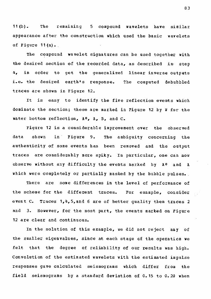
83

11(b). The remaining 5 compound wavelets have s i m i l a r

appearance a f t e r the construction which used the basic wavelets

of Figure 11 (a).

The compound wavelet signatures can be used together with

the desired section of the recorded data, as described in- step

4, i n order to get the generalized l i n e a r inverse outputs

i . e . the desired earth's response. The computed debubbled

traces are shown in Figure 12.

It i s easy to i d e n t i f y the f i v e r e f l e c t i o n events which

dominate the section; these are marked i n Figure 12 by W for the

water bottom r e f l e c t i o n , A°, A, B, and C.

Figure 12 i s a considerable improvement over the observed

data shown i n Figure 9. The ambiguity concerning the

authenticity of some events has been removed and the output

traces are considerably more spiky. In p a r t i c u l a r , one can now

observe without any d i f f i c u l t y the events marked by A° and A

which were completely or p a r t i a l l y masked by the bubble pulses.

There are some differences i n the l e v e l of performance of

the scheme for the d i f f e r e n t traces. For example, consider

event C. Traces 1,4,5,and 6 are of better quality then traces 2

and 3. However, for the most part, the events marked on Figure

12 are clear and continuous.

In the solution of t h i s example, we did not r e j e c t any of

the smaller eigenvalues, since at each stage cf the operation we

f e l t that the degree of r e l i a b i l i t y of our r e s u l t s was high.

Convolution of the estimated wavelets with the estimated impulse

responses gave calculated seismograms which d i f f e r from the

f i e l d seismograms by a standard deviation of 0.15 to 0.20 when

83a

F i g u r e 12 - The estimated impulse response set (debubbled

seismograms) c a l c u l a t e d by the g e n e r a l i z e d l i n e a r i n v e r s e scheme.

The p o l a r i t y r e v e r s a l of the output response i n the f i f t h t r a c e

(offset, i s about 1.4 km) i s due t o the phase s h i f t e d wavelet.

R e f l e c t i o n events are marked b y W, A°, A, B and C.

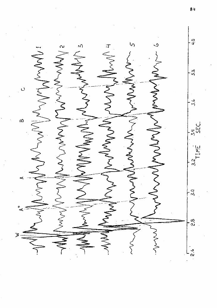
84

85

normalized to a maximum amplitude of 1. We f e e l that such a

standard deviation i s acceptable and the debubbled traces are a

better representation of the earth's response function, thereby

enabling a better interpretation.

CONCLUSION

The generalized l i n e a r inverse scheme has been shown to be

a useful t o o l for wavelet estimation and debubbling. We

estimated the wavelet and used t h i s estimate i n cur debubbling-

signature compression procedure.

An attempt to deconvolve a trace given an error-

contaminated wavelet by using Weiner f i l t e r s or by d i v i d i n g the

trace's Fourier transform by that of the given wavelet w i l l

often re s u l t i n erroneous outputs. We believe that the method

described i n t h i s work increases the processor's a b i l i t y to deal

with noisy wavelets.

An important advantage of the generalized l i n e a r inverse

scheme i s that one does not (and can not) solve for the impulse

response exactly. Rather, one gets the l e a s t sguares solution.

Since a l l of the eguations i n the deconvolution problem are

weighted egually, the presence of errors i n some of them w i l l

not necessarily re s u l t i n erroneous solutions. Furthermore,

using the properties discussed in Chapter 3, we are able to

solve the deconvolution problem to within a prespecified

standard deviation, provided that t h i s standard deviation i s

86

consistent with the given problem (one cannot get out of the

data more then i t has). The smallest standard deviation

(S.D)min i s achieved when a l l the eigenvalues are kept i n the

solution of eguation (6). However, i f (S.D) min i s small

compared to the estimated noise l e v e l , the mechanism of small

eigenvalues rejec t i o n can be used. This mechanism allows us to

solve problems with highly noisy observations, or highly ncisy

wavelets (see Chapter 3) .

The proposed scheme treats debubbling and signature

compression i n one step and thus reduces the r i s k of accumulated

error. (Although the singular value decomposition process i s a

time consuming one, i t seems to be reasonably stable).

Since the wavelet signature within the same trace i s time

dependent, one may expect that an inverse f i l t e r , calculated for

a ce r t a i n time i n t e r v a l , may not perform acceptably i n another

time i n t e r v a l along the trace. The generalized l i n e a r inverse

scheme i s more f l e x i b l e to errors i n the wavelet and hence we

expect that given a ce r t a i n wavelet, the inversion scheme w i l l

be able to be used successfully over a longer time i n t e r v a l .

An important consideration i n our scheme i s the singular

value decomposition process, which i s a time consuming one and

hence increases the cost of the inversion. In order to reduce

the size of the problem, one has to increase the d i g i t i z a t i o n

i n t e r v a l , which i n turn might reduce the solution's guality.

However, i n many cases the data are d i g i t i z e d at smaller

i n t e r v a l s than what i s r e a l l y necessary. In such cases,

increasing the d i g i t i z a t i o n i n t e r v a l w i l l r e s u l t i n considerable

saving without any reduction i n solution quality. In the f i e l d

87

example d i s c r i b e d above, we i n c r e a s e d the d i g i t i z a t i o n i n t e r v a l

from 0.0032 sec to 0.0096 sec, i n c l u d e d 2.0 sec of observed data

with a 0.6 sec wavelet and obtained a response output of l e n g t h

1.4 sec. Even with t h i s data decimation, a matrix of the c r d e r

of 200 by 140 had to be i n v e r t e d .

Our work and others (D.W. Oldenberg, p e r s o n a l

comunication, 1979), suggests l i n e a r i n v e r s e methods may be

q u i t e s u c c e s s f u l i n t r e a t i n g d e c o n v o l u t i o n problems i n which

nois e i s p r e v a l e n t . Then, i n cases where r e g u l a r time s e r i e s

a n a l y s i s technigues do not g i v e a c c e p t a b l e r e s u l t s , the more

co m p u t a t i o n a l l y expensive i n v e r s i o n a l g o r i t h m s could be a p p l i e d .

In t h i s study we have approached the debubbling procedure

as a g e n e r a l i z e d l i n e a r i n v e r s e problem. As d i s c u s s e d i n

Chapter 3, an a l t e r n a t i v e approach i n which the problem can be

formulated i s the B a c k u s - G i l b e r t technique. The a p p l i c a t i o n of

t h i s procedure might g i v e even b e t t e r r e s u l t s than those shown

i n t h i s study.

8 8

REFERENCES

Clayton R.Wr McClary 5., and Wiggins E.A., 1976. E u l l .

Seism. Soc. Am. , 66, 325-326.

Clowes B.M., 1977. A marine deep seismic sounding system,

Can. J. Earth S c i . , 14, 1276-1285.

Clowes E. M., Thorleifson A.J., and Lynch S., 1978.

Interpretation of a marine deep seismic sounding survey i n

Winona Basin off the West Coast of Canada, Gecl. Surv. Can.

Paper 78-1C, 29-34.

Harman H.H., 1960. Modern factor analysis, Dniv. Of

Chicago Press, Chicago.

Inman J.E., Eyu J . , and Ward S.H., 1973. B e s i s t i v i t y

inversion, Geophysics, 38, 1088-1108.

Jackson D. D., 1972. Interpretation cf inaccurate,

i n s u f f i c i e n t and inconsistent data, Geophys. J. B. Astr.

Soc., 28,

Kramer F.S., Peterson B.A., and Walters W.C, 1968.

Seismic energy sources 1968 handbook. United Geophysical

Corporation, 57p.

Lanczos C., 1961. Linear d i f f e r e n t i a l operators, D. Van

Nostrand Co., London.

Lines L.E., and Ulrych T.J., 1977. The old and the new i n

seismic deconvolution and wavelet estimation, Geophys. Prosp.,

25, 512-540.

Mateker E.J., 1971. Big benefits seen with maxipulse

system use. O i l and Gas J . , 69, 116-120.

89

Ooe M.r and Ulrych T.J., 1979. Minimum entropy

deconvolution with an exponential transformation, Geophys.

Prosp. (in press).

Robinson E.A., 1967. Multichannel time series analysis

with d i g i t a l computer programs, Holden-Day, San Francisco.

Thorleifson A.J., 1978. A marine deep seismic sounding

survey over Winona Basin, M. Ap. Sc.. Thesis, Univ. Of B r i t i s h

Columbia, 70p.

T r e i t e l S., and Robinson E.A., 1966. The design of high

resolution d i g i t a l f i l t e r s , IEE Trans., Geosci. Electronics GE-

4, 25-38.

Ulrych T.J., Walker C.J., and Jurkevics A.J., 1978. A

f i l t e r length c r i t e r i o n for minimum entropy deconvolution, J .

Can. Soc. Expl. Geophys.,14, 21-28.

Wiggins R.A., Larner K.L., and Wisecup R.D., 1976.

Residual s t a t i c s analysis as a general l i n e a r inverse problem,

Geophysics, 41, 922-933.

Wiggins R.A., 1977. Minimum entropy deconvolution, Proc.

Int. Symp. computer aided seismic analysis and discrimination,

Falmouth, Mass., IEEE Computer Society, 7-14.

Wiggins R.A., Helmberger D.V., 1974. Synthetic seismograms

by expansion i n generalized rays, Geophys. J . R. Astr. S o c ,

37, 73-90.