Wavelet-based Image Compression - People Pages: …people.uwec.edu/walkerjs/media/imagecompchap.pdf · Wavelet-based Image Compression ... Our purpose in discussing the baseline compression

Wavelet-based Image Compression

Sub-chapter of CRC Press book: Transforms and Data Compression

James S. WalkerDepartment of Mathematics

University of Wisconsin–Eau ClaireEau Claire, WI 54702–4004

Phone: 715–836–3301Fax: 715–836–2924

e-mail: [email protected]

1 Image compression

There are two types of image compression: lossless and lossy. With losslesscompression, the original image is recovered exactly after decompression.Unfortunately, with images of natural scenes it is rarely possible to obtainerror-free compression at a rate beyond 2:1. Much higher compression ratioscan be obtained if some error, which is usually difficult to perceive, is allowedbetween the decompressed image and the original image. This is lossy com-pression. In many cases, it is not necessary or even desirable that there beerror-free reproduction of the original image. For example, if some noise ispresent, then the error due to that noise will usually be significantly reducedvia some denoising method. In such a case, the small amount of error intro-duced by lossy compression may be acceptable. Another application wherelossy compression is acceptable is in fast transmission of still images over theInternet.

We shall concentrate on wavelet-based lossy compression of grey-level stillimages. When there are 256 levels of possible intensity for each pixel, then weshall call these images 8 bpp (bits per pixel) images. Images with 4096 grey-levels are referred to as 12 bpp. Some brief comments on color images willalso be given, and we shall also briefly describe some wavelet-based losslesscompression methods.

1.1 Lossy compression

The methods of lossy compression that we shall concentrate on are the follow-ing: the EZW algorithm, the SPIHT algorithm, the WDR algorithm, andthe ASWDR algorithm. These are relatively recent algorithms which achievesome of the lowest errors per compression rate and highest perceptual qualityyet reported. After describing these algorithms in detail, we shall list someof the other algorithms that are available.

Before we examine the algorithms listed above, we shall outline the basicsteps that are common to all wavelet-based image compression algorithms.The five stages of compression and decompression are shown in Figs. 1 and2. All of the steps shown in the compression diagram are invertable, hencelossless, except for the Quantize step. Quantizing refers to a reduction ofthe precision of the floating point values of the wavelet transform, which aretypically either 32-bit or 64-bit floating point numbers. To use less bits inthe compressed transform—which is necessary if compression of 8 bpp or 12

1

bpp images is to be achieved—these transform values must be expressed withless bits for each value. This leads to rounding error. These approximate,quantized, wavelet transforms will produce approximations to the imageswhen an inverse transform is performed. Thus creating the error inherent inlossy compression.

Image →WaveletTransform

→ Quantize ↔ Encode →CompressedImage

Figure 1: Compression of an image

CompresssedImage

→ Decode ↔ApproximateWaveletTransform

→InverseWaveletTransform

→Round off tointeger values,create Image

Figure 2: Decompression of an image

The relationship between the Quantize and the Encode steps, shown inFig. 1, is the crucial aspect of wavelet transform compression. Each of thealgorithms described below takes a different approach to this relationship.

The purpose served by the Wavelet Transform is that it produces a largenumber of values having zero, or near zero, magnitudes. For example, con-sider the image shown in Fig. 3(a), which is called Lena. In Fig. 3(b), weshow a 7-level Daub 9/7 wavelet transform of the Lena image. This transformhas been thresholded, using a threshold of 8. That is, all values whose mag-nitudes are less than 8 have been set equal to 0, they appear as a uniformlygrey background in the image in Fig. 3(b). These large areas of grey back-ground indicate that there is a large number of zero values in the thresholdedtransform. If an inverse wavelet transform is performed on this thresholdedtransform, then the image in Fig. 3(c) results (after rounding to integer val-ues between 0 and 255). It is difficult to detect any difference between theimages in Figs. 3(a) and (c).

The image in Fig. 3(c) was produced using only the 32, 498 non-zero valuesof the thresholded transform, instead of all 262, 144 values of the original

2

(a) (b) (c)

Figure 3: (a) Lena image, 8 bpp. (b) Wavelet transform of image, threshold= 8. (c) Inverse of thresholded wavelet transform, PSNR = 39.14 dB.

transform. This represents an 8:1 compression ratio. We are, of course,ignoring difficult problems such as how to transmit concisely the positions ofthe non-zero values in the thresholded transform, and how to encode thesenon-zero values with as few bits as possible. Solutions to these problems willbe described below, when we discuss the various compression algorithms.

Two commonly used measures for quantifying the error between imagesare Mean Square Error (MSE) and Peak Signal to Noise Ratio (PSNR). TheMSE between two images f and g is defined by

MSE =1

N

∑

j,k

(f [j, k] − g[j, k])2 (1)

where the sum over j, k denotes the sum over all pixels in the images, and Nis the number of pixels in each image. For the images in Figs. 3(a) and (c),the MSE is 7.921. The PSNR between two (8 bpp) images is, in decibels,

PSNR = 10 log10

(

2552

MSE

)

. (2)

PSNR tends to be cited more often, since it is a logarithmic measure, andour brains seem to respond logarithmically to intensity. Increasing PSNRrepresents increasing fidelity of compression. For the images in Figs. 3(a)and (c), the PSNR is 39.14 dB. Generally, when the PSNR is 40 dB or larger,then the two images are virtually indistinguishable by human observers. Inthis case, we can see that 8:1 compression should yield an image almost

3

identical to the original. The methods described below do in fact producesuch results, with even greater PSNR than we have just achieved with ourcrude approach.

3 4

1 2

9 10

12 11

13 14

15 16

5 8

6 7

48 47 46 45

41 42 43 44

40 39 38 37

33 34 35 36

58 59 63 64

52 57 60 62

51 53 56 61

49 50 54 55

20 21 28 29

19 22 27 30

18 23 26 31

17 24 25 32

(a) 2-level

3 4

1 2

9 10

12 11

13 14

15 16

5 8

6 7

48 47 46 45

41 42 43 44

40 39 38 37

33 34 35 36

58 59 63 64

52 57 60 62

51 53 56 61

49 50 54 55

20 21 28 29

19 22 27 30

18 23 26 31

17 24 25 32

(b) 3-level

Figure 4: Scanning for wavelet transforms: zigzag through all-lowpass sub-band, column scan through vertical subbands, row scan through horizontalsubbands, zigzag through diagonal subbands. (a) and (b): Order of scannedelements for 2-level and 3-level transforms of 8 by 8 image.

Before we begin our treatment of various “state of the art” algorithms, itmay be helpful to briefly outline a “baseline” compression algorithm of thekind described in [1] and [2]. This algorithm has two main parts.

First, the positions of the significant transform values—the ones havinglarger magnitudes than the threshold T—are determined by scanning throughthe transform as shown in Fig. 4. The positions of the significant values arethen encoded using a run-length method. To be precise, it is necessary tostore the values of the significance map:

s(m) ={

0 if |w(m)| < T1 if |w(m)| ≥ T ,

(3)

where m is the scanning index, and w(m) is the wavelet transform value atindex m. From Fig. 3(b) we can see that there will be long runs of s(m) = 0.If the scan order illustrated in Fig. 4 is used, then there will also be long

4

runs of s(m) = 1. The positions of significant values can then be conciselyencoded by recording sequences of 6-bits according to the following pattern:

0 a b c d e: run of 0 of length (a b c d e)2

1 a b c d e: run of 1 of length (a b c d e)2.

A lossless compression, such as Huffman or arithmetic compression, of thesedata is also performed for a further reduction in bits.

Second, the significant values of the transform are encoded. This can bedone by dividing the range of transform values into subintervals (bins) androunding each transform value into the midpoint of the bin in which it lies.In Fig. 5 we show the histogram of the frequencies of significant transformvalues lying in 512 bins for the 7-level Daub 9/7 transform of Lena shownin Fig. 3(b). The extremely rapid drop in the frequencies of occurrenceof higher transform magnitudes implies that the very low-magnitude values,which occur much more frequently, should be encoded using shorter length bitsequences. This is typically done with either Huffman encoding or arithmeticcoding. If arithmetic coding is used, then the average number of bits neededto encode each significant value in this case is about 1 bit.

Figure 5: Histogram for 512 bins for thresholded transform of Lena

We have only briefly sketched the steps in this baseline compression al-gorithm. More details can be found in [1] and [2].

Our purpose in discussing the baseline compression algorithm was to in-troduce some basic concepts, such as scan order and thresholding, which areneeded for our examination of the algorithms to follow. The baseline algo-rithm was one of the first to be proposed using wavelet methods [3]. It suffers

5

from some defects which later algorithms have remedied. For instance, withthe baseline algorithm it is very difficult, if not impossible, to specify in ad-vance the exact compression rate or the exact error to be achieved. This is aserious defect. Another problem with the baseline method is that it does notallow for progressive transmission. In other words, it is not possible to sendsuccessive data packets (over the Internet, say) which produce successivelyincreased resolution of the received image. Progressive transmission is vitalfor applications that include some level of interaction with the receiver.

Let us now turn to these improved wavelet image compression algorithms.The algorithms to be discussed are the EZW algorithm, the SPIHT algo-rithm, the WDR algorithm, and the ASWDR algorithm.

1.2 EZW algorithm

The EZW algorithm was one of the first algorithms to show the full powerof wavelet-based image compression. It was introduced in the groundbreak-ing paper of Shapiro [4]. We shall describe EZW in some detail because asolid understanding of it will make it much easier to comprehend the otheralgorithms we shall be discussing. These other algorithms build upon thefundamental concepts that were first introduced with EZW.

Our discussion of EZW will be focused on the fundamental ideas underly-ing it; we shall not use it to compress any images. That is because it has beensuperseded by a far superior algorithm, the SPIHT algorithm. Since SPIHTis just a highly refined version of EZW, it makes sense to first describe EZW.

EZW stands for Embedded Zerotree Wavelet. We shall explain the termsEmbedded, and Zerotree, and how they relate to Wavelet-based compression.An embedded coding is a process of encoding the transform magnitudes thatallows for progressive transmission of the compressed image. Zerotrees area concept that allows for a concise encoding of the positions of significantvalues that result during the embedded coding process. We shall first discussembedded coding, and then examine the notion of zerotrees.

The embedding process used by EZW is called bit-plane encoding. Itconsists of the following five-step process:

Bit-plane encoding

Step 1 (Initialize). Choose initial threshold, T = T0, such that all transformvalues satisfy |w(m)| < T0 and at least one transform value satisfies |w(m)| ≥T0/2.

6

Step 2 (Update threshold). Let Tk = Tk−1/2.

Step 3 (Significance pass). Scan through insignificant values using baselinealgorithm scan order. Test each value w(m) as follows:

If |w(m)| ≥ Tk, then

Output sign of w(m)

Set wQ(m) = Tk

Else if |w(m)| < Tk then

Let wQ(m) retain its initial value of 0.

Step 4 (Refinement pass). Scan through significant values found with higherthreshold values Tj , for j < k (if k = 1 skip this step). For each significantvalue w(m), do the following:

If |w(m)| ∈ [wQ(m), wQ(m) + Tk), then

Output bit 0

Else if |w(m)| ∈ [wQ(m) + Tk, wQ(m) + 2Tk), then

Output bit 1

Replace value of wQ(m) by wQ(m) + Tk.

Step 5 (Loop). Repeat steps 2 through 4.

This bit-plane encoding procedure can be continued for as long as necessaryto obtain quantized transform magnitudes wQ(m) which are as close as de-sired to the transform magnitudes |w(m)|. During decoding, the signs andthe bits output by this method can be used to construct an approximatewavelet transform to any desired degree of accuracy. If instead, a given com-pression ratio is desired, then it can be achieved by stopping the bit-planeencoding as soon as a given number of bits (a bit budget) is exhausted. Ineither case, the execution of the bit-plane encoding procedure can terminateat any point (not just at the end of one of the loops).

As a simple example of bit-plane encoding, suppose that we just have twotransform values w(1) = −9.5 and w(2) = 42. For an initial threshold, we setT0 = 64. During the first loop, when T1 = 32, the output is the sign of w(2),and the quantized transform magnitudes are wQ(1) = 0 and wQ(2) = 32.For the second loop, T2 = 16, and there is no output from the significancepass. The refinement pass produces the bit 0 because w(2) ∈ [32, 32 + 16).The quantized transform magnitudes are wQ(1) = 0 and wQ(2) = 32. During

7

the third loop, when T3 = 8, the significance pass outputs the sign of w(1).The refinement pass outputs the bit 1 because w(2) ∈ [32 + 8, 32 + 16). Thequantized transform magnitudes are wQ(1) = 8 and wQ(2) = 40.

It is not hard to see that after n loops, the maximum error between the

transform values and their quantized counterparts is less than T0/2n. It fol-

lows that we can reduce the error to as small a value as we wish by performinga large enough number of loops. For instance, in the simple example justdescribed, with seven loops the error is reduced to zero. The output fromthese seven loops, arranged to correspond to w(1) and w(2), is

w(1): − 0 0 1 1w(2): + 0 1 0 1 0 0

Notice that w(2) requires seven symbols, but w(1) only requires five.Bit-plane encoding simply consists of computing binary expansions—

using T0 as unit—for the transform values and recording in magnitude order

only the significant bits in these expansions. Because the first significant bitis always 1, it is not encoded. Instead the sign of the transform value isencoded first. This coherent ordering of encoding, with highest magnitudebits encoded first, is what allows for progressive transmission.

Wavelet transforms are particularly well-adapted for bit-plane encoding.1

This is because wavelet transforms of images of natural scenes often haverelatively few high-magnitude values, which are mostly found in the highestlevel subbands. These high-magnitude values are first coarsely approximatedduring the initial loops of the bit-plane encoding. Thereby producing a low-resolution, but often recognizable, version of the image. Subsequent loopsencode lower magnitude values and refine the high magnitude values. Thisadds further details to the image and refines existing details. Thus progres-sive transmission is possible, and encoding/decoding can cease once a givenbit budget is exhausted or a given error target is achieved.

Now that we have described the embedded coding of wavelet transformvalues, we shall describe the zerotree method by which EZW transmits thepositions of significant transform values. The zerotree method gives an im-plicit, very compact, description of the location of significant values by cre-ating a highly compressed description of the location of insignificant values.For many images of natural scenes, such as the Lena image for example,insignificant values at a given threshold T are organized in zerotrees.

1Although other transforms, such as the block Discrete Cosine Transform, can also bebit-plane encoded.

8

To define a zerotree we first define a quadtree. A quadtree is a tree oflocations in the wavelet transform with a root [i, j], and its children locatedat [2i, 2j], [2i+1, 2j], [2i, 2j+1], and [2i+1, 2j+1], and each of their children,and so on. These descendants of the root reach all the way back to the 1st levelof the wavelet transform. For example, in Fig. 6(a), we show two quadtrees(enclosed in dashed boxes). One quadtree has root at index 12 and childrenat indices {41, 42, 47, 48}. This quadtree has two levels. We shall denote it by{12 | 41, 42, 47, 48}. The other quadtree, which has three levels, has its root atindex 4, the children of this root at indices {13, 14, 15, 16}, and their childrenat indices {49, 50, . . . , 64}. It is denoted by {4 | 13, . . . , 16 | 49, . . . , 64}.

Now that we have defined a quadtree, we can give a simple definitionof a zerotree. A zerotree is a quadtree which, for a given threshold T , has

insignificant wavelet transform values at each of its locations. For example,if the threshold is T = 32, then each of the quadtrees shown in Fig. 6(a) is azerotree for the wavelet transform in Fig. 6(b). But if the threshold is T = 16,then {12 | 41, 42, 47, 48} remains a zerotree, but {4 | 13, . . . , 16 | 49, . . . , 64} isno longer a zerotree because its root value is no longer insignificant.

Zerotrees can provide very compact descriptions of the locations of in-significant values because it is only necessary to encode one symbol, R say,to mark the root location. The decoder can infer that all other locationsin the zerotree have insignificant values, so their locations are not encoded.

For the threshold T = 32, in the example just discussed, two R symbols areenough to specify all 26 locations in the two zerotrees.

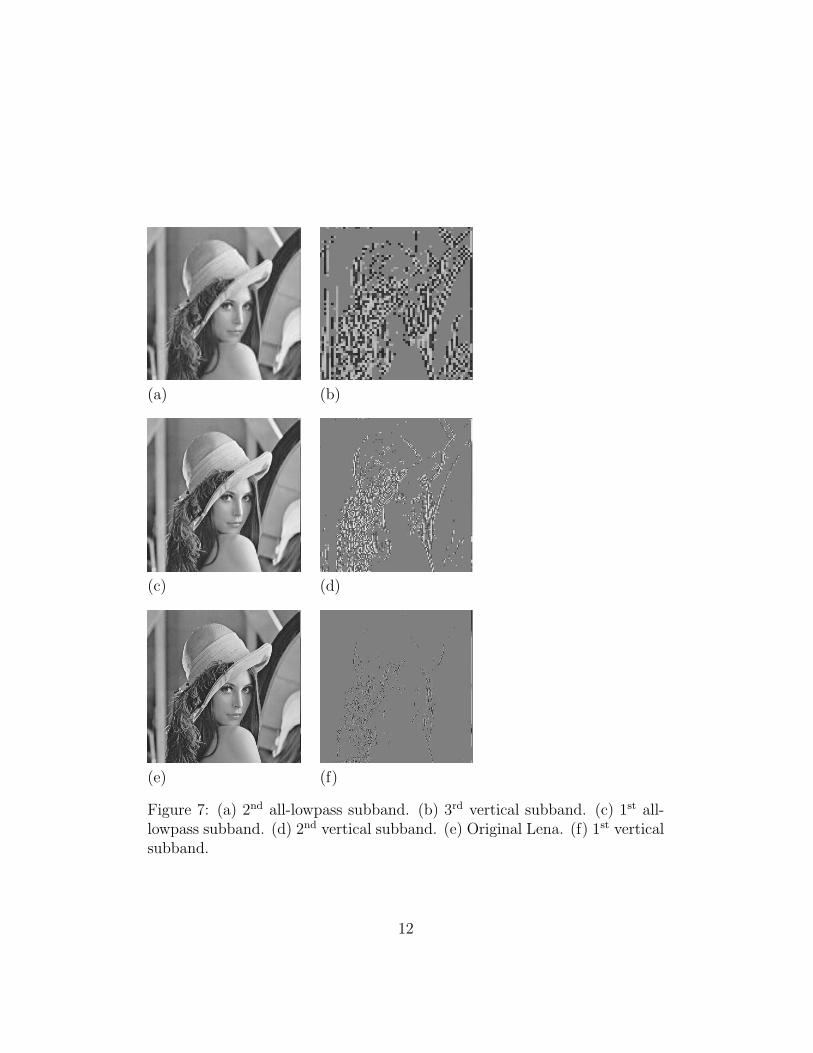
Zerotrees can only be useful if they occur frequently. Fortunately, withwavelet transforms of natural scenes, the multiresolution structure of thewavelet transform does produce many zerotrees (especially at higher thresh-olds). For example, consider the images shown in Fig. 7. In Fig. 7(a) we showthe 2nd all-lowpass subband of a Daub 9/7 transform of the Lena image. Theimage 7(b) on its right is the 3rd vertical subband produced from this all-lowpass subband, with a threshold of 16. Notice that there are large patchesof grey pixels in this image. These represent insignificant transform valuesfor the threshold of 16. These insignificant values correspond to regions ofnearly constant, or nearly linearly graded, intensities in the image in 7(a).Such intensities are nearly orthogonal to the analyzing Daub 9/7 wavelets.Zerotrees arise for the threshold of 16 because in image 7(c)—the 2nd all-lowpass subband—there are similar regions of constant or linearly gradedintensities. In fact, it was precisely these regions which were smoothed anddownsampled to create the corresponding regions in image 7(a). These re-

9

3 4

1 2

9 10

12 11

13 14

15 16

5 8

6 7

48 47 46 45

41 42 43 44

40 39 38 37

33 34 35 36

58 59 63 64

52 57 60 62

51 53 56 61

49 50 54 55

20 21 28 29

19 22 27 30

18 23 26 31

17 24 25 32

(a) Scan order, with two quadtrees

63 −34

−31 23

49 10

14 −13

−9 14

−25 −7

3 −12

−14 8

5 11 5 6

2 −3 6 −4

3 0 −3 2

−5 9 −1 47

0 3 −4 4

3 6 3 6

3 −2 0 4

4 6 −2 2

4 −2 3 2

5 −7 3 9

3 4 6 −1

5 18 −12 7

(b) Wavelet transform

+ −

I R

+ R

R R

R I

R R

• •

• •

• • • •

• • • •

• • I I

• • I +

• • • •

• • • •

• • • •

• • • •

• • • •

• • • •

I I • •

I I • •

(c) Threshold = 32

+ −

− +

+ R

R R

− R

R R

R R

R R

• • • •

• • • •

I I • •

I I • +

• • • •

• • • •

• • • •

• • • •

• • • •

• • • •

I I • •

I + • •

(d) Threshold = 16

Figure 6: First two stages of EZW. (a) 3-level scan order. (b) 3-level wavelettransform. (c) Stage 1, threshold = 32. (d) Stage 2, threshold = 16.

10

gions in image 7(c) produce insignificant values in the same relative locations

(the child locations) in the 2nd vertical subband shown in image 7(d).Likewise, there are uniformly grey regions in the same relative locations

in the 1st vertical subband [see Fig. 7(f)]. Because the 2nd vertical subband inFig. 7(d) is magnified by a factor of two in each dimension, and the 3rd verticalsubband in 7(b) is magnified by a factor of four in each dimension, it followsthat the common regions of grey background shown in these three verticalsubbands are all zerotrees. Similar images could be shown for horizontal anddiagonal subbands, and they would also indicate a large number of zerotrees.

The Lena image is typical of many images of natural scenes, and the abovediscussion gives some background for understanding how zerotrees arise inwavelet transforms. A more rigorous, statistical discussion can be found inShapiro’s paper [4].

Now that we have laid the foundations of zerotree encoding, we can com-plete our discussion of the EZW algorithm. The EZW algorithm simplyconsists of replacing the significance pass in the Bit-plane encoding pro-cedure with the following step:

EZW Step 3 (Significance pass). Scan through insignificant values usingbaseline algorithm scan order. Test each value w(m) as follows:

If |w(m)| ≥ Tk, then

Output the sign of w(m)

Set wQ(m) = Tk


Let wQ(m) remain equal to 0

If m is at 1st level, then

Output I

Else

Search through quadtree having root m

If this quadtree is a zerotree, then

Output R

Else

Output I.

During a search through a quadtree, values that were found to be significantat higher thresholds are treated as zeros. All descendants of a root of azerotree are skipped in the rest of the scanning at this threshold.

11

(a) (b)

(c) (d)

(e) (f)

Figure 7: (a) 2nd all-lowpass subband. (b) 3rd vertical subband. (c) 1st all-lowpass subband. (d) 2nd vertical subband. (e) Original Lena. (f) 1st verticalsubband.

12

As an example of the EZW method, consider the wavelet transform shownin Fig. 6(b), which will be scanned through using the scan order shown inFig. 6(a). Suppose that the initial threshold is T0 = 64. In the first loop, thethreshold is T1 = 32. The results of the first significance pass are shown inFig. 6(c). The coder output after this first loop would be

+ − I R + R R R R I R R I I I I I + I I (4)

corresponding to a quantized transform having just two values: ±32. With+32 at each location marked by a plus sign in Fig. 6(c), and −32 at eachlocation marked by a minus sign, and 0 at all other locations. In the secondloop, with threshold T2 = 16, the results of the significance pass are indicatedin Fig. 6(d). Notice, in particular, that there is a symbol R at the position 11in the scan order. That is because the plus sign which lies at a child locationis from the previous loop, so it is treated as zero. Hence position 11 is at theroot of a zerotree. There is also a refinement pass done in this second loop.The output from this second loop is then

− + R R R − R R R R R R R I I I + I I I I 1 0 1 0 (5)

with corresponding quantized wavelet transform shown in Fig. 8(a). TheMSE between this quantized transform and the original transform is 48.6875.This is a 78% reduction in error from the start of the method (when thequantized transform has all zero values).

A couple of final remarks are in order concerning the EZW method. First,it should be clear from the discussion above that the decoder, whose structureis outlined in Fig. 2 above, can reverse each of the steps of the coder andproduce the quantized wavelet transform. It is standard practice for thedecoder to then round the quantized values to the midpoints of the intervalsthat they were last found to belong to during the encoding process (i.e., addhalf of the last threshold used to their magnitudes). This generally reducesMSE. For instance, in the example just considered, if this rounding is doneto the quantized transform in Fig. 8(a), then the result is shown in Fig. 8(b).The MSE is then 39.6875, a reduction of more than 18%. A good discussionof the theoretical justification for this rounding technique can be found in[2]. This rounding method will be employed by all of the other algorithms that

we shall discuss.

Second, since we live in a digital world, it is usually necessary to transmitjust bits. A simple encoding of the symbols of the EZW algorithm into bits

13

48 −32

−16 16

48 0

0 0

−16 0

0 0

0 0

0 0

0 0 0 0

0 0 0 0

0 0 0 0

0 0 0 32

0 0 0 0

0 0 0 0

0 0 0 0

0 0 0 0

0 0 0 0

0 0 0 0

0 0 0 0

0 16 0 0

(a)

56 −40

−24 24

56 0

0 0

−24 0

0 0

0 0

0 0

0 0 0 0

0 0 0 0

0 0 0 0

0 0 0 40

0 0 0 0

0 0 0 0

0 0 0 0

0 0 0 0

0 0 0 0

0 0 0 0

0 0 0 0

0 20 0 0

(b)

Figure 8: (a) Quantization at end of 2nd stage, MSE = 48.6875. (b) Afterrounding to midpoints, MSE = 39.6875, reduction by more than 18%.

would be to use a code such as P = 0 1, N = 0 0, R = 1 0, and I = 1 1. Sincethe decoder can always infer precisely when the encoding of these symbolsends (the significance pass is complete), the encoding of refinement bits cansimply be as single bits 0 and 1. This form of encoding is the fastest toperform, but it does not achieve the greatest compression. In [4], a losslessform of arithmetic coding was recommended in order to further compress thebit stream from the encoder.

1.3 SPIHT algorithm

The SPIHT algorithm is a highly refined version of the EZW algorithm.It was introduced in [5] and [6] by Said and Pearlman. Some of the bestresults—highest PSNR values for given compression ratios—for a wide vari-ety of images have been obtained with SPIHT. Consequently, it is probablythe most widely used wavelet-based algorithm for image compression, pro-viding a basic standard of comparison for all subsequent algorithms.

SPIHT stands for Set Partitioning in Hierarchical Trees. The term Hi-

erarchical Trees refers to the quadtrees that we defined in our discussion ofEZW. Set Partitioning refers to the way these quadtrees divide up, partition,

14

the wavelet transform values at a given threshold. By a careful analysis ofthis partitioning of transform values, Said and Pearlman were able to greatlyimprove the EZW algorithm, significantly increasing its compressive power.

Our discussion of SPIHT will consist of three parts. First, we shall de-scribe a modified version of the algorithm introduced in [5]. We shall referto it as the Spatial-orientation Tree Wavelet (STW) algorithm. STW is es-sentially the SPIHT algorithm, the only difference is that SPIHT is slightlymore careful in its organization of coding output. Second, we shall describethe SPIHT algorithm. It will be easier to explain SPIHT using the conceptsunderlying STW. Third, we shall see how well SPIHT compresses images.

The only difference between STW and EZW is that STW uses a differentapproach to encoding the zerotree information. STW uses a state transition

model. From one threshold to the next, the locations of transform valuesundergo state transitions. This model allows STW to reduce the number ofbits needed for encoding. Instead of code for the symbols R and I output byEZW to mark locations, the STW algorithm uses states IR, IV , SR, and SV

and outputs code for state-transitions such as IR → IV , SR → SV , etc. Todefine the states involved, some preliminary definitions are needed.

For a given index m in the baseline scan order, define the set D(m) asfollows. If m is either at the 1st level or at the all-lowpass level, then D(m) isthe empty set ∅. Otherwise, if m is at the jth level for j > 1, then

D(m) = {Descendents of index m in quadtree with root m}.

The significance function S is defined by

S(m) =

maxn∈D(m)

|w(n)|, if D(m) 6= ∅

∞, if D(m) = ∅.

With these preliminary definitions in hand, we can now define the states.For a given threshold T , the states IR, IV , SR, and SV are defined by

m ∈ IR if and only if |w(m)| < T, S(m) < T (6)

m ∈ IV if and only if |w(m)| < T, S(m) ≥ T (7)

m ∈ SR if and only if |w(m)| ≥ T, S(m) < T (8)

m ∈ SV if and only if |w(m)| ≥ T, S(m) ≥ T. (9)

In Fig. 9, we show the state transition diagram for these states when a

15

IV SV

IR SR-

-? ?

@@

@@@R

j

j j

j

Figure 9: State transition diagram for STW

threshold is decreased from T to T ′ < T . Notice that once a location marrives in state SV , then it will remain in that state. Furthermore, there areonly two transitions from each of the states IV and SR, so those transitionscan be coded with one bit each. A simple binary coding for these statetransitions is shown in Table 1.

Old\New IR IV SR SV

IR 00 01 10 11IV 0 1SR 0 1SV •

Table 1: Code for state transitions, • indicates that SV → SV transition iscertain (hence no encoding needed).

Now that we have laid the groundwork for the STW algorithm, we cangive its full description.

STW encoding

Step 1 (Initialize). Choose initial threshold, T = T0, such that all transformvalues satisfy |w(m)| < T0 and at least one transform value satisfies |w(m)| ≥T0/2. Assign all indices for the Lth level, where L is the number of levelsin the wavelet transform, to the dominant list (this includes all locationsin the all-lowpass subband as well as the horizontal, vertical, and diagonalsubbands at the Lth level). Set the refinement list of indices equal to theempty set.


16

Step 3 (Dominant pass). Use the following procedure to scan throughindices in the dominant list (which can change as the procedure is executed).

Do

Get next index m in dominant list

Save old state Sold = S(m, Tk−1)

Find new state Snew = S(m, Tk) using (6)-(9)

Output code for state transition Sold → Snew

If Snew 6= Sold then do the following

If Sold 6= SR and Snew 6= IV then

Append index m to refinement list

Output sign of w(m) and set wQ(m) = Tk

If Sold 6= IV and Snew 6= SR then

Append child indices of m to dominant list

If Snew = SV then

Remove index m from dominant list

Loop until end of dominant list

Step 4 (Refinement pass). Scan through indices m in the refinement listfound with higher threshold values Tj , for j < k (if k = 1 skip this step).For each value w(m), do the following:


Output bit 0


Output bit 1



To see how STW works—and how it improves the EZW method—it helpsto reconsider the example shown in Fig. 6. In Fig. 10, we show STW statesfor the wavelet transform in Fig. 6(b) using the same two thresholds as weused previously with EZW. It is important to compare the three quadtreesenclosed in the dashed boxes in Fig. 10 with the corresponding quadtreesin Figs. 6(c) and (d). There is a large savings in coding output for STWrepresented by these quadtrees. The EZW symbols for these three quadtrees

17

are + I I I I, − I I I I, and + R R R R. For STW, however, they are describedby the symbols + SR, −SR, and + SR, which is a substantial reduction inthe information that STW needs to encode.

SV SV

IV IR

SR IR

IR IR

IR IV

IR IR

• •

• •

• • • •

• • • •

• • IV IV

• • IV SV

• • • •

• • • •

• • • •

• • • •

• • • •

• • • •

• • • •

• • • •

(a) Threshold = 32

SV SV

SV SR

SV IR

IR IR

SR IV

IR IR

• •

• •

• • • •

• • • •

• • IV IV

• • IV SV

• • • •

• • • •

• • • •

• • • •

• • • •

• • • •

IV IV • •

IV SV • •

(b) Threshold = 16

Figure 10: First two stages of STW for wavelet transform in Fig. 6.

There is not much difference between STW and SPIHT. The one thingthat SPIHT does differently is to carefully organize the output of bits in theencoding of state transitions in Table 1, so that only one bit is output at a

time. For instance, for the transition IR → SR, which is coded as 1 0 inTable 1, SPIHT outputs a 1 first and then (after further processing) outputsa 0. Even if the bit budget is exhausted before the second bit can be output,the first bit of 1 indicates that there is a new significant value.

The SPIHT encoding process, as described in [6], is phrased in termsof pixel locations [i, j] rather than indices m in a scan order. To avoidintroducing new notation, and to highlight the connections between SPIHTand the other algorithms, EZW and STW, we shall rephrase the descriptionof SPIHT from [6] in term of scanning indices. We shall also slightly modifythe notation used in [6] in the interests of clarity.

First, we need some preliminary definitions. For a given set I of indicesin the baseline scan order, the significance ST [I] of I relative to a threshold

18

T is defined by

ST [I] =

1, if maxn∈I

|w(n)| ≥ T

0, if maxn∈I

|w(n)| < T .(10)

It is important to note that, for the initial threshold T0, we have ST0[I] = 0

for all sets of indices. If I is a set containing just a single index m, then forconvenience we shall write ST [m] instead of ST [{m}].

For a succinct presentation of the method, we need the following defini-tions of sets of indices:

D(m) = {Descendent indices of the index m}

C(m) = {Child indices of the index m}

G(m) = D(m) − C(m)

= {Grandchildren of m, i.e., descendants which are not children}.

In addition, the set H consists of indices for the Lth level, where L is thenumber of levels in the wavelet transform (this includes all locations in theall-lowpass subband as well as the horizontal, vertical, and diagonal subbandsat the Lth level). It is important to remember that the indices in the all-lowpass subband have no descendants. If m marks a location in the all-lowpass subband, then D(m) = ∅.

SPIHT keeps track of the states of sets of indices by means of three lists.They are the list of insignificant sets (LIS), the list of insignificant pixels

(LIP), and the list of significant pixels (LSP). For each list a set is identifiedby a single index, in the LIP and LSP these indices represent the singletonsets {m} where m is the identifying index. An index m is called eithersignificant or insignificant, depending on whether the transform value w(m)is significant or insignificant with respect to a given threshold. For the LIS,

the index m denotes either D(m) or G(m). In the former case, the index m issaid to be of type D and, in the latter case, of type G.

The following is pseudocode for the SPIHT algorithm. For simplicity, weshall write the significance function STk

as Sk.

SPIHT encoding

Step 1 (Initialize). Choose initial threshold T0 such that all transformvalues satisfy |w(m)| < T0 and at least one value satisfies |w(m)| ≥ T0/2.Set LIP equal to H, set LSP equal to ∅, and set LIS equal to all the indicesin H that have descendants (assigning them all type D).

19


Step 3 (Sorting pass). Proceed as follows:

For each m in LIP do:

Output Sk[m]

If Sk[m] = 1 then

Move m to end of LSP

Output sign of w(m); set wQ(m) = Tk

Continue until end of LIP

For each m in LIS do:

If m is of type D then

Output Sk[D(m)]

If Sk[D(m)] = 1 then

For each n ∈ C(m) do:

Output Sk[n]

If Sk[n] = 1 then

Append n to LSP

Output sign of w(n); set wQ(n) = Tk

Else If Sk[n] = 0 then

Append n to LIP

If G(m) 6= ∅ then

Move m to end of LIS as type G

Else

Remove m from LIS

Else If m is of type G then

Output Sk[G(m)]

If Sk[G(m)] = 1 then

Append C(m) to LIS, all type D indices

Remove m from LIS

Continue until end of LIS

Notice that the set LIS can undergo many changes during this procedure, ittypically does not remain fixed throughout.

Step 4 (Refinement pass). Scan through indices m in LSP found with higher

20

threshold values Tj , for j < k (if k = 1 skip this step). For each value w(m),do the following:


Output bit 0


Output bit 1



It helps to carry out this procedure on the wavelet transform shown in Fig. 6.Then one can see that SPIHT simply performs STW with the binary code for

the states in Table 1 being output one bit at a time.

Now comes the payoff. We shall see how well SPIHT performs in com-pressing images. To do these compressions we used the public domain SPIHTprograms from [7]. In Fig. 11 we show several SPIHT compressions of theLena image. The original Lena image is shown in Fig. 11(f). Five SPIHTcompressions are shown with compression ratios of 128:1, 64:1, 32:1, 16:1,and 8:1.

There are several things worth noting about these compressed images.First, they were all produced from one file, the file containing the 1 bppcompression of the Lena image. By specifying a bit budget, a certain bppvalue up to 1, the SPIHT decompression program will stop decoding the 1bpp compressed file once the bit budget is exhausted. This illustrates theembedded nature of SPIHT.

Second, the rapid convergence of the compressed images to the originalis nothing short of astonishing. Even the 64: 1 compression in Fig. 11(b) isalmost indistinguishable from the original. A close examination of the twoimages is needed in order to see some differences, e.g., the blurring of detailsin the top of Lena’s hat. The image in (b) would be quite acceptable forsome applications, such as the first image in a sequence of video telephoneimages or as a thumbnail display within a large archive.

Third, notice that the 1 bpp image has a 40.32 dB PSNR value andis virtually indistinguishable—even under very close examination—from theoriginal. Here we find that SPIHT is able to exceed the simple thresholdingcompression we first discussed (see Fig. 3). For reasons of space, we cannotshow SPIHT compressions of many test images, so in Table 2 we give PSNR

21

(a) 0.0625 bpp (128:1) (b) 0.125 bpp (64:1) (c) 0.25 bpp (32:1)

(d) 0.5 bpp (16:1) (e) 1.0 bpp (8:1) (f) Original, 8 bpp

Figure 11: SPIHT compressions of Lena image. PSNR values: (a) 27.96 dB.(b) 30.85 dB. (c) 33.93 dB. (d) 37.09 dB. (e) 40.32 dB.

values for several test images [8]. These data show that SPIHT produceshigher PSNR values than the two other algorithms that we shall describebelow. SPIHT is well-known for its superior performance when PSNR is usedas the error measure. High PSNR values, however, are not the sole criteriafor the performance of lossy compression algorithms. We shall discuss othercriteria below.

Fourth, these SPIHT compressed images were obtained using SPIHT’sarithmetic compression option. The method that SPIHT uses for arithmeticcompression is quite involved and space does not permit a discussion of thedetails here. Some details are provided in [9].

Finally, it is interesting to compare SPIHT compressions with compres-

22

Image/Method SPIHT WDR ASWDRLena, 0.5 bpp 37.09 36.45 36.67Lena, 0.25 bpp 33.85 33.39 33.64Lena, 0.125 bpp 30.85 30.42 30.61Goldhill, 0.5 bpp 33.10 32.70 32.85Goldhill, 0.25 bpp 30.49 30.33 30.34Goldhill, 0.125 bpp 28.39 28.25 28.23Barbara, 0.5 bpp 31.29 30.68 30.87Barbara, 0.25 bpp 27.47 26.87 27.03Barbara, 0.125 bpp 24.77 24.30 24.52Airfield, 0.5 bpp 28.57 28.12 28.36Airfield, 0.25 bpp 25.90 25.49 25.64Airfield, 0.125 bpp 23.68 23.32 23.50

Table 2: PSNR values, with arithmetic compression

sions obtained with the JPEG method.2 The JPEG method is a sophisticatedimplementation of block Discrete Cosine Transform encoding [10]. It is usedextensively for compression of images, especially for transmission over theInternet. In Fig. 12, we compare compressions of the Lena image obtainedwith JPEG and with SPIHT at three different compression ratios. (JPEGdoes not allow for specifying the bpp value in advance; the 59:1 compressionwas the closest we could get to 64:1.) It is clear from these images thatSPIHT is far superior to JPEG. It is better both in perceptual quality andin terms of PSNR. Notice, in particular, that the 59:1 JPEG compression isvery distorted (exhibiting “blocking” artifacts stemming from coarse quan-tization within the blocks making up the block DCT used by JPEG). TheSPIHT compression, even at the slightly higher ratio of 64:1, exhibits noneof these objectionable features. In fact, for quick transmission of a thumb-nail image (say, as part of a much larger webpage), this SPIHT compressionwould be quite acceptable. The 32:1 JPEG image might be acceptable forsome applications, but it also contains some blocking artifacts. The 32:1SPIHT compression is almost indistinguishable (at these image sizes) fromthe original Lena image. The 16:1 compressions for both methods are nearly

2JPEG stands for Joint Photographic Experts Group, a group of engineers who devel-oped this compression method.

23

indistinguishable. In fact, they are both nearly indistinguishable from theoriginal Lena image.

Although we have compared JPEG with SPIHT using only one image, theresults we have found are generally valid. SPIHT compressions are superiorto JPEG compressions both in perceptual quality and in PSNR values. Infact, all of the wavelet-based image compression techniques that we discusshere are superior to JPEG. Hence, we shall not make any further comparisonswith the JPEG method.

(a) JPEG 59:1 (b) JPEG 32:1 (c) JPEG 16:1

(d) SPIHT 64:1 (e) SPIHT 32:1 (f) SPIHT 16:1

Figure 12: Comparison of JPEG and SPIHT compressions of Lena image.PSNR values: (a) 24.16 dB. (b) 30.11 dB. (c) 34.12 dB. (d) 30.85 dB. (e)33.93 dB. (f) 37.09 dB.

24

1.4 WDR Algorithm

One of the defects of SPIHT is that it only implicitly locates the positionof significant coefficients. This makes it difficult to perform operations, suchas region selection on compressed data, which depend on the exact positionof significant transform values. By region selection, also known as region of

interest (ROI), we mean selecting a portion of a compressed image whichrequires increased resolution. This can occur, for example, with a portion ofa low resolution medical image that has been sent at a low bpp rate in orderto arrive quickly.

Such compressed data operations are possible with the Wavelet Difference

Reduction (WDR) algorithm of Tian and Wells [11]–[13]. The term difference

reduction refers to the way in which WDR encodes the locations of significantwavelet transform values, which we shall describe below. Although WDR willnot typically produce higher PSNR values than SPIHT (see Table 2), we shallsee that WDR can produce perceptually superior images, especially at highcompression ratios.

The only difference between WDR and the Bit-plane encoding de-scribed above is in the significance pass. In WDR, the output from the sig-nificance pass consists of the signs of significant values along with sequencesof bits which concisely describe the precise locations of significant values.The best way to see how this is done is to consider a simple example.

Suppose that the significant values are w(2) = +34.2, w(3) = −33.5,w(7) = +48.2, w(12) = +40.34, and w(34) = −54.36. The indices for thesesignificant values are 2, 3, 7, 12, and 34. Rather than working with thesevalues, WDR works with their successive differences: 2, 1, 4, 5, 22. In thislatter list, the first number is the starting index and each successive numberis the number of steps needed to reach the next index. The binary expansionsof these successive differences are (10)2, (1)2, (100)2, (101)2, and (10110)2.Since the most significant bit for each of these expansions is always 1, this bitcan be dropped and the signs of the significant transform values can be usedinstead as separators in the symbol stream. The resulting symbol stream forthis example is then +0 − +00 + 01 − 0110.

When this most significant bit is dropped, we shall refer to the binaryexpansion that remains as the reduced binary expansion. Notice, in partic-ular, that the reduced binary expansion of 1 is empty. The reduced binaryexpansion of 2 is just the 0 bit, the reduced binary expansion of 3 is just the1 bit, and so on.

25

The WDR algorithm simply consists of replacing the significance pass inthe Bit-plane encoding procedure with the following step:

WDR Step 3 (Significance pass). Perform the following procedure on theinsignificant indices in the baseline scan order:

Initialize step-counter C = 0

Let Cold = 0

Do

Get next insignificant index m

Increment step-counter C by 1

If |w(m)| ≥ Tk then

Output sign w(m) and set wQ(m) = Tk

Move m to end of sequence of significant indices

Let n = C − Cold

Set Cold = C

If n > 1 then

Output reduced binary expansion of n



Loop until end of insignificant indices

Output end-marker

The output for the end-marker is a plus sign, followed by the reduced binaryexpansion of n = C + 1 − Cold, and a final plus sign.

It is not hard to see that WDR is of no greater computational complexitythan SPIHT. For one thing, WDR does not need to search through quadtreesas SPIHT does. The calculations of the reduced binary expansions adds somecomplexity to WDR, but they can be done rapidly with bit-shift operations.As explained in [11]–[13], the output of the WDR encoding can be arithmeti-cally compressed. The method that they describe is based on the elementaryarithmetic coding algorithm described in [14]. This form of arithmetic codingis substantially less complex (at the price of poorer performance) than thearithmetic coding employed by SPIHT.

As an example of the WDR algorithm, consider the scan order and wavelettransform shown in Fig. 6. For the threshold T1 = 32, the significant values

26

are w(1) = 63, w(2) = −34, w(5) = 49, and w(36) = 47. The output of theWDR significance pass will then be the following string of symbols:

+ − + 1 + 1 1 1 1 + 1 1 0 1 +

which compares favorably with the EZW output in Eq. (4). The last sixsymbols are the code for the end-marker. For the threshold T2 = 16, the newsignificant values are w(3) = −31, w(4) = 23, w(9) = −25, and w(24) = 18.Since the previous indices 1, 2, 5, and 36, are removed from the sequence ofinsignificant indices, the values of n in the WDR significance pass will be 1,1, 4, and 15. In this case, the value of n for the end-marker is 40. Adding onthe four refinement bits, which are the same as in Eq. (5), the WDR outputfor this second threshold is

− + − 0 0 + 1 1 1 + 0 1 0 0 0 + 1 0 1 0

which is also a smaller output than the corresponding EZW output. It isalso clear that, for this simple case, WDR does not produce as compact anoutput as STW does.

As an example of WDR performance for a natural image, we show inFig. 13 several compressions of the Lena image. These compressions wereproduced with the free software [15].

There are a couple things to observe about these compressions. First,the PSNR values are lower than for SPIHT. This is typically the case. InTable 2 we compare PSNR values for WDR and for SPIHT on several imagesat various compression ratios. In every case, SPIHT has higher PSNR values.

Second, at high compression ratios, the visual quality of WDR compres-sions of Lena are superior to those of SPIHT. For example, the 0.0625 bppand 0.125 bpp compressions have higher resolution with WDR. This is easierto see if the images are magnified as in Fig. 14. At 0.0625 bpp, the WDRcompression does a better job in preserving the shape of Lena’s nose and inretaining some of the striping in the band around her hat. Similar remarksapply to the 0.125 bpp compressions. SPIHT, however, does a better job inpreserving parts of Lena’s eyes. These observations point to the need for anobjective, quantitative measure of image quality.

There is no universally accepted objective measure for image quality. Weshall now describe a simple measure that we have found useful. There is someevidence that the visual system of humans concentrates on analyzing edges inimages [16], [17]. To produce an image that retains only edges, we proceed as

27

(a) 0.0625 bpp (128:1) (b) 0.125 bpp (64:1) (c) 0.25 bpp (32:1)


Figure 13: WDR compressions of Lena image. PSNR values: (a) 27.63 dB.(b) 30.42 dB. (c) 33.39 dB. (d) 36.45 dB. (e) 39.62 dB.

follows. First, a 3-level Daub 9/7 transform of an image f is created. Second,the all-lowpass subband is subtracted away from this transform. Third, aninverse transform is performed on the remaining part of the transform. Thisproduces a highpass filtered image, which exhibits edges from the image f . Asimilar highpass filtered image is created from the compressed image. Bothof these highpass filtered images have mean values that are approximatelyzero. We define the edge correlation γ3 by

γ3 =σc

σo

where σc denotes the standard deviation of the values of the highpass filteredversion of the compressed image, and σo denotes the standard deviation of thevalues of the highpass filtered version of the original image. Thus γ3 measures

28

(a) Original (b) SPIHT, 0.0625 bpp (c) WDR, 0.0625 bpp

(d) Original (e) SPIHT, 0.125 bpp (f) WDR, 0.125 bpp

Figure 14: SPIHT and WDR compressions of Lena at low bpp.

how well the compressed image captures the variation of edge details in theoriginal image.

Using this edge correlation measure, we obtained the results shown in Ta-ble 3. In every case, the WDR compressions exhibit higher edge correlationsthan the SPIHT compressions. These numerical results are also consistentwith the increased preservation of details within WDR images, and with theinformal reports of human observers.

Although WDR is simple, competitive with SPIHT in PSNR values, andoften provides better perceptual results, there is still room for improvement.We now turn to a recent enhancement of the WDR algorithm.

29

Image/Method SPIHT WDR ASWDRLena, 0.5 bpp .966 .976 .978Lena, 0.25 bpp .931 .946 .951Lena, 0.125 bpp .863 .885 .894Goldhill, 0.5 bpp .920 .958 .963Goldhill, 0.25 bpp .842 .870 .871Goldhill, 0.125 bpp .747 .783 .781Barbara, 0.5 bpp .932 .955 .959Barbara, 0.25 bpp .861 .894 .902Barbara, 0.125 bpp .739 .767 .785Airfield, 0.5 bpp .922 .939 .937Airfield, 0.25 bpp .857 .871 .878Airfield, 0.125 bpp .766 .790 .803

Table 3: Edge correlations, with arithmetic compression

1.5 ASWDR algorithm

One of the most recent image compression algorithms is the Adaptively

Scanned Wavelet Difference Reduction (ASWDR) algorithm of Walker [18].The adjective adaptively scanned refers to the fact that this algorithm modi-fies the scanning order used by WDR in order to achieve better performance.

ASWDR adapts the scanning order so as to predict locations of newsignificant values. If a prediction is correct, then the output specifying thatlocation will just be the sign of the new significant value—the reduced binaryexpansion of the number of steps will be empty. Therefore a good predictionscheme will significantly reduce the coding output of WDR.

The prediction method used by ASWDR is the following: If w(m) is sig-

nificant for threshold T , then the values of the children of m are predicted to

be significant for half-threshold T/2. For many natural images, this predic-tion method is a reasonably good one. As an example, in Fig. 15 we showtwo vertical subbands for a Daub 9/7 wavelet transform of the Lena image.The image in Fig. 15(a) is of those significant values in the 2nd level ver-tical subband for a threshold of 16 (significant values shown in white). InFig. 15(b), we show the new significant values in the 1st vertical subband forthe half-threshold of 8. Notice that there is a great deal of similarity in thetwo images. Since the image in Fig. 15(a) is magnified by two in each dimen-

30

(a) (b)

Figure 15: (a) Significant values, 2nd vertical subband, threshold 16. (b) New

significant values, 1st vertical subband, threshold 8.

sion, its white pixels actually represent the predictions for the locations ofnew significant values in the 1st vertical subband. Although these predictionsare not perfectly accurate, there is a great deal of overlap between the twoimages. Notice also how the locations of significant values are highly corre-lated with the location of edges in the Lena image. The scanning order ofASWDR dynamically adapts to the locations of edge details in an image, andthis enhances the resolution of these edges in ASWDR compressed images.

A complete validation of the prediction method just described would re-quire assembling statistics for a large number of different subbands, differentthresholds, and different images. Rather than attempting such an a priori

argument (see [19]), we shall instead argue from an a posteriori standpoint.We shall present statistics that show that the prediction scheme employed byASWDR does, in fact, encode more significant values than are encoded byWDR for a number of different images. As the pseudocode presented belowwill show, the only difference between ASWDR and WDR is in the predictivescheme employed by ASWDR to create new scanning orders. Consequently,if ASWDR typically encodes more values than WDR does, this must be dueto the success of the predictive scheme.

In Table 4 we show the numbers of significant values encoded by WDRand ASWDR for four different images. In almost every case, ASWDR wasable to encode more values than WDR. This gives an a posteriori validationof the predictive scheme employed by ASWDR.

We now present the pseudocode description of ASWDR encoding. Notice

31

Image\Method WDR ASWDR % increaseLena, 0.125 bpp 5, 241 5, 458 4.1%Lena, 0.25 bpp 10, 450 11, 105 6.3%Lena, 0.5 bpp 20, 809 22, 370 7.5%Goldhill, 0.125 bpp 5, 744 5, 634 −1.9%Goldhill, 0.25 bpp 10, 410 10, 210 −1.9%Goldhill, 0.5 bpp 22, 905 23, 394 2.1%Barbara, 0.125 bpp 5, 348 5, 571 4.2%Barbara, 0.25 bpp 11, 681 12, 174 4.2%Barbara, 0.5 bpp 23, 697 24, 915 5.1%Airfield, 0.125 bpp 5, 388 5, 736 6.5%Airfield, 0.25 bpp 10, 519 11, 228 6.7%Airfield, 0.5 bpp 19, 950 21, 814 9.3%

Table 4: Number of significant values encoded, no arithmetic coding

that the significance pass portion of this procedure is the same as the WDRsignificance pass described above, and that the refinement pass is the sameas for Bit-plane encoding (hence the same as for WDR). The one newfeature is the insertion of a step for creating a new scanning order.

ASWDR encoding

Step 1 (Initialize). Choose initial threshold, T = T0, such that all transformvalues satisfy |w(m)| < T0 and at least one transform value satisfies |w(m)| ≥T0/2. Set the initial scan order to be the baseline scan order.


Step 3 (Significance pass). Perform the following procedure on the insignif-icant indices in the scan order:

Initialize step-counter C = 0

Let Cold = 0

Do

Get next insignificant index m

Increment step-counter C by 1

If |w(m)| ≥ Tk then

32

(a) 0.0625 bpp (128:1) (b) 0.125 bpp (64:1) (c) 0.25 bpp (32:1)


Figure 16: ASWDR compressions of Lena image. PSNR values: (a) 27.73dB. (b) 30.61 dB. (c) 33.64 dB. (d) 36.67 dB. (e) 39.90 dB.

Output sign w(m) and set wQ(m) = Tk

Move m to end of sequence of significant indices

Let n = C − Cold

Set Cold = C

If n > 1 then

Output reduced binary expansion of n



Loop until end of insignificant indices

Output end-marker as per WDR Step 3

33

Step 4 (Refinement pass). Scan through significant values found with higherthreshold values Tj , for j < k (if k = 1 skip this step). For each significantvalue w(m), do the following:


Output bit 0


Output bit 1


Step 5 (Create new scan order). For each level j in the wavelet transform(except for j = 1), scan through the significant values using the old scanorder. The initial part of the new scan order at level j − 1 consists of theindices for insignificant values corresponding to the child indices of theselevel j significant values. Then, scan again through the insignificant valuesat level j using the old scan order. Append to the initial part of the newscan order at level j − 1 the indices for insignificant values corresponding tothe child indices of these level j significant values. Note: No change is madeto the scan order at level L, where L is the number of levels in the wavelettransform.


The creation of the new scanning order only adds a small degree of com-plexity to the original WDR algorithm. Moreover, ASWDR retains all of theattractive features of WDR: simplicity, progressive transmission capability,and ROI capability.

In Fig. 16 we show how ASWDR performs on the Lena image. ThePSNR values for these images are slightly better than those for WDR, andalmost as good as those for SPIHT. More importantly, the perceptual qualityof ASWDR compressions are better than SPIHT compressions and slightlybetter than WDR compressions. This is especially true at high compressionratios. In Fig. 17 we show magnifications of 128:1 and 64:1 compressionsof the Lena image. The ASWDR compressions better preserve the shape ofLena’s nose, and details of her hat, and show less distortion along the side ofher left cheek (especially for the 0.125 bpp case). These subjective observa-tions are borne out by the edge correlations in Table 3. In almost every case,the ASWDR compressions produce slightly higher edge correlation values.

As a further example of the superior performance of ASWDR at highcompression ratios, in Fig. 18 we show compressions of the Airfield image at

34

(a) SPIHT (b) WDR (c) ASWDR

(d) SPIHT (e) WDR (f) ASWDR

Figure 17: SPIHT, WDR, and ASWDR compressions of Lena at low bpp.(a)–(c) 0.0625 bpp, 128:1. (d)–(f) 0.125 bpp, 64:1.

128:1. The WDR and ASWDR algorithms preserve more of the fine detailsin the image. Look especially along the top of the images: SPIHT erasesmany fine details such as the telephone pole and two small square structuresto the right of the thin black rectangle. These details are preserved, at leastpartially, by both WDR and ASWDR. The ASWDR image does the best jobin retaining some structure in the telephone pole. ASWDR is also superiorin preserving the structure of the swept-back winged aircraft, especially itsthin nose, located to the lower left of center. These are only a few of themany details in the airplane image which are better preserved by ASWDR.

As quantitative support for the superiority of ASWDR in preserving edgedetails, we show in Table 5 the values for three different edge correlations γk,k = 3, 4, and 5. Here k denotes how many levels in the Daub 9/7 wavelet

35

(a) Original (b) SPIHT

(c) WDR (d) ASWDR

Figure 18: Comparisons of 128:1 compressions of airfield image

transform were used. A higher value of k means that edge detail at lowerresolutions was considered in computing the edge correlation. These edgecorrelations show that ASWDR is superior over several resolution levels inpreserving edges in the airfield image at the low bit rate of 0.0625 bpp.

High compression ratio images like these are used in reconnaissance andin medical applications, where fast transmission and ROI (region selection)are employed, as well as multi-resolution detection. The WDR and ASWDRalgorithms do allow for ROI while SPIHT does not. Furthermore, theirsuperior performance in displaying edge details at low bit rates facilitatesmulti-resolution detection.

Further research is being done on improving the ASWDR algorithm. Oneimportant enhancement will be the incorporation of an improved predictive

36

Corr./Method SPIHT WDR ASWDRγ3 .665 .692 .711γ4 .780 .817 .827γ5 .845 .879 .885

Table 5: Edge correlations for 128:1 compressions of Airfield image

scheme, based on weighted values of neighboring transform magnitudes asdescribed in [19].

1.6 Lossless compression

A novel aspect of the compression/decompression methods diagrammed inFigs. 1 and 2 is that integer-to-integer wavelet transforms can be used in placeof the ordinary wavelet transforms (such as Daub 9/7) described so far. Aninteger-to-integer wavelet transform produces an integer-valued transformfrom the grey-scale, integer-valued image [20]. Since n loops in Bit-planeencoding reduces the quantization error to less than T0/2

n, it follows thatonce 2n is greater than T0, there will be zero error. In other words, thebit-plane encoded transform will be exactly the same as the original wavelettransform, hence lossless encoding is achieved (with progressive transmissionas well). Of course, for many indices, the zero error will occur sooner thanwith the maximum number of loops n. Consequently, some care is neededin order to efficiently encode the minimum number of bits in each binaryexpansion. A discussion of how SPIHT is adapted to achieve lossless encodingcan be found in [9]. The algorithms WDR and ASWDR can also be adaptedin order to achieve lossless encoding, but public versions of such adaptationsare not yet available. (When they are released, they will be accessible at[15].)

1.7 Color images

Following the standard practice in image compression research, we have con-centrated here on methods of compressing grey-scale images. For color im-ages, this corresponds to compressing the intensity portion of the image.That is, if the color image is a typical RGB image, with 8 bits for Red,8 bits for Green, and 8 bits for Blue, then the intensity I is defined by

37

I = (R + B + G)/3, which rounds to an 8-bit grey-scale image. The humaneye is most sensitive to variations in intensity, so the most difficult part ofcompressing a color image lies in the compressing of the intensity. Usually,the two color “channels” are denoted Y and C and are derived from the R,G, and B values [21]. Much greater compression can be done on the Y and Cversions of the image, since the human visual system is much less sensitive tovariations in these two variables. Each of the algorithms described above canbe modified so as to compress color images. For example, the public domainSPIHT coder [7] does provide programs for compressing color images. Forreasons of space, we cannot describe compression of color images in any moredetail.

1.8 Other compression algorithms

There are a wide variety of wavelet-based image compression algorithms be-sides the ones that we focused on here. Some of the most promising arealgorithms that minimize the amount of memory which the encoder and/ordecoder must use, see [22] and [23]. A new algorithm which is embedded andwhich minimizes PSNR is described in [24]. Many other algorithms are citedin the review article [1]. In evaluating the performance of any new imagecompression algorithm, one must take into account not only PSNR values,but also consider the following factors: (1) perceptual quality of the images(edge correlation values can be helpful here), (2) whether the algorithm allowsfor progressive transmission, (3) the complexity of the algorithm (includingmemory usage), and (4) whether the algorithm has ROI capability.

References

[1] G.M. Davis, A. Nosratinia. Wavelet-based Image Coding: An Overview.Applied and Computational Control, Signals and Circuits, Vol. 1, No. 1,1998.

[2] S. Mallat. A Wavelet Tour of Signal Processing. Academic Press, NewYork, NY, 1998.

[3] M. Antonini, M. Barlaud, P. Mathieu, I. Daubechies. Image coding usingwavelet transform. IEEE Trans. Image Proc., Vol. 5, No. 1, pp. 205-220,1992.

38

[4] J.M. Shapiro. Embedded image coding using zerotrees of wavelet coeffi-cients. IEEE Trans. Signal Proc., Vol. 41, No. 12, pp. 3445–3462, 1993.

[5] A. Said, W.A. Pearlman. Image compression using the spatial-orientationtree. IEEE Int. Symp. on Circuits and Systems, Chicago, IL, pp. 279–282,1993.

[6] A. Said, W.A. Pearlman. A new, fast, and efficient image codec based onset partitioning in hierarchical trees. IEEE Trans. on Circuits and Systems

for Video Technology, Vol. 6, No. 3, pp. 243–250, 1996.

[7] SPIHT programs can be downloaded from ftp://ipl.rpi.edu/pub/.

[8] Go to ftp://ipl.rpi.edu/pub/image/still/usc/gray/ for Lena, Gold-hill, and Barbara. Go to http://www.image.cityu.edu.hk/imagedb/ forAirfield.

[9] A. Said, W.A. Pearlman. An image multi-resolution representation for loss-less and lossy image compression. IEEE Trans. Image Proc., Vol. 5, No. 9,pp. 1303–1310, 1996.

[10] G.K. Wallace. The JPEG still picture compression standard. Comm. of the

ACM, Vol. 34, No. 4, pp. 30–44, 1991.

[11] J. Tian, R.O. Wells, Jr. A lossy image codec based on index coding. IEEE

Data Compression Conference, DCC ’96, page 456, 1996.

[12] J. Tian, R.O. Wells, Jr. Embedded image coding using wavelet-difference-reduction. Wavelet Image and Video Compression, P. Topiwala, ed.,pp. 289–301. Kluwer Academic Publ., Norwell, MA, 1998.

[13] J. Tian, R.O. Wells, Jr. Image data processing in the compressed waveletdomain. 3rd International Conference on Signal Processing Proc., B. Yuanand X. Tang, Eds., pp. 978–981, Beijing, China, 1996.

[14] I. Witten, R. Neal, J. Cleary. Arithmetic coding for data compression.Comm. of the ACM, Vol. 30, No. 6, pp. 1278–1288, 1986.

[15] WDR and ASWDR compressors are part of the FAWAV software packageat http://www.crcpress.com/edp/download/fawav/fawav.htm/

[16] D. Marr, Vision. W.H. Freeman, San Francisco, CA, 1982.

39

[17] M.G. Ramos, S.S. Hemami, Activity selective SPIHT coding. Proc. SPIE

3653, Visual Communications and Image Processing ’99, San Jose, CA,Jan. 1999. See also errata for this paper athttp://foulard.ee.cornell.edu/marcia/asspiht2.html.

[18] J.S. Walker. A lossy image codec based on adaptively scanned waveletdifference reduction. Submitted to Optical Engineering.

[19] R.W. Buccigrossi, E.P. Simoncelli, Image compression via joint statisti-cal characterization in the wavelet domain. IEEE Trans. on Image Proc.,

Vol. 8, No. 12, 1999.

[20] A.R. Calderbank, I. Daubechies, W. Sweldens, B.-L. Yeo, Wavelet trans-forms that map integers to integers. Applied and Computational Harmonic

Analysis, Vol. 5, No. 3, pp. 332-369, 1998.

[21] J.C. Russ, The Image Processing Handbook. CRC Press, Boca Raton, FL,1995.

[22] A. Islam, W.A. Pearlman, An embedded and efficient low-complexity hier-archical image coder. Proc. SPIE 3653, Visual Communications and Image

Processing ’99, San Jose, CA, Jan. 1999.

[23] H. Malvar, Progressive wavelet coding of images. Proc. of IEEE Data Com-

pression Conference, Salt Lake City, UT, pp. 336–343, March, 1999.

[24] J. Li, S. Lei, An embedded still image coder with rate-distortion optimiza-tion. IEEE Trans. on Image Proc., Vol. 8, No. 7, pp. 913–924, 1999.

40

Documents

Wavelet-based Image Compression - People Pages: …people.uwec.edu/walkerjs/media/imagecompchap.pdf · Wavelet-based Image Compression ... Our purpose in discussing the baseline compression