Wave propagation in anisotropic media with non-local ... · Wave propagation in anisotropic media with non ... local elasticity on the wave propagation ... analysis in anisotropic

International Journal of Solids and Structures 44 (2007) 5723–5741

www.elsevier.com/locate/ijsolstr

Wave propagation in anisotropic media with non-local elasticity

A. Chakraborty *

India Science Lab, GM Technical Centre (I) Bangalore 560066, Karnataka, India

Received 22 June 2006; received in revised form 22 January 2007; accepted 22 January 2007Available online 26 January 2007

Abstract

In an effort to understand and quantify the effect of non-local elasticity on the wave propagation response of laminatedcomposite layered media, a frequency-wavenumber domain based finite element method is employed. The developed ele-ments are based on the exact solution in the transformed domain and thus exactly represent the dynamics of a layer. Thisfeature enables to model a layer of any thickness by a single element and drastically reduces the cost of computation. Theeffect of non-locality on the dispersion relation and in turn on the wave response is compared with local (classical) elasticitysolutions. A procedure and sample example is outlined to estimate the magnitude of the non-locality parameter by com-paring the dispersion relation with lattice dynamics. The effect of non-locality, in terms of the mode-shift and appearanceof dispersion on the modes of Lamb waves is further demonstrated.� 2007 Elsevier Ltd. All rights reserved.

Keywords: Non-local elasticity; Wave propagation; Spectral finite element; Lamb wave

1. Introduction

All engineering materials posses intrinsic length scales in terms of their repetitive atomic or molecular struc-tures. The classical theory of elasticity, which is commonly used to explain the behavior of these materials,however, does not accommodate any such scale. The absence of the length scale creates several discrepanciesin the predictions of mechanical responses, e.g., infinite stress field near crack tip or non-dispersive wavebehavior (constant wave speed, independent of frequency). For example, according to the classical elasticity,Rayleigh waves propagating on the surface of a semi-infinite isotropic elastic space are non-dispersive in nat-ure (Love, 1944), whereas, experiments and the atomic theory of lattice predict otherwise. These anomaliesindicate the limitations of the classical theory of elasticity and stress the need for molecular dynamics(MD) based simulations.

However, modern practical problems are still intractable for MD based analysis, even if the highest com-puting facility is at disposal. Hence, refinement of the existing continuum theory for the purpose of more real-istic predictions seems to be the only viable alternative. Several attempts have been made so far in thisdirection, e.g., the non-local theory of elasticity (Eringen, 1976) and the peridynamic theory (Silling, 2000)

0020-7683/$ - see front matter � 2007 Elsevier Ltd. All rights reserved.

doi:10.1016/j.ijsolstr.2007.01.024

* Fax: +91 080 41158562.E-mail address: [email protected]

mailto:[email protected]

5724 A. Chakraborty / International Journal of Solids and Structures 44 (2007) 5723–5741

where the objective is always to modify the stress gradient term in the governing momentum equilibrium equa-tions so that the long-range effects are taken into account. In the case of the non-local theory of Eringen, thelong-range effect is considered by modifying the stress-strain relation as a convolution of the elastic modulusover strain as

rijðxÞ ¼Z

Xðkðx� yÞ þ 2lðx� yÞÞ�ijðyÞ þ kðx� yÞ�kkðyÞdij dX; ð1Þ

instead of the point-wise relationship of the classical elasticity theory. The domain X signifies the range of theinter-atomic forces. On the other hand, the peridynamic theory modifies the governing equation as

q€u ¼Z

Xf ðx� y; uðx; tÞ � uðy; tÞÞdX: ð2Þ

These approaches pose different level of complexities when it comes to the solution of the governing equations.The non-local theory generates singular perturbed partial differential equation, whereas, the peridynamic the-ory involves integro-differential equation with no spatial derivatives. Thus, the solution strategy becomes moreinvolved in the later case. In this work, the non-local theory of Eringen is used to develop wave solutions foranisotropic media.

Non-local elasticity involves spatial variation of the elastic moduli, where the dependency is dictated by a sin-gular non-local kernel. For example, gaussian kernel has been used by Eringen for analyzing screw and edge dis-locations (Eringen, 1976, 1977). These kernels should satisfy a number of criteria, which are given in the nextsection. Additionally, these kernels can be taken as the Greens functions of the Helmholtz equation, which arestudied by Eringen (1983, 1992, 2002). Similar investigations are carried out by various other researchers to elim-inate stress singularities (see Lazar et al., 2006). However, in this work, the main concern is the issues involved inthe wave propagation analysis in the domain of non-local elasticity, which is discussed next.

One important outcome of the non-local elasticity is the realistic prediction of the dispersion curve (i.e.,frequency-wavenumber/wavevector relation). As shown in Eringen (1987), the dispersion relation

x=c1k ¼ ð1þ �2k2Þ�1=2; � ¼ Nonlocality parameter; ð3Þ

closely matches with the Born–Karman model dispersion

xa=c1 ¼ 2 sinðka=2Þ; ð4Þ

when � = 0.39a is considered. However, among the two natural conditions at the mid-point and end of the firstBrillouin zone:

dx=dkjðk¼0Þ ¼ c1; dx=dkjðk¼p=aÞ ¼ 0; ð5Þ

the relation in Eq. (3) satisfies only the first one. It was suggested that two-parameter approximation of thekernel function will give better results. This is reiterated by Lazar et al. (2006) that one parameter (only �)non-local kernel will never be able to model the lattice dynamics relation and it is necessary to use thebi-Helmholtz type equation with two different coefficients of non-locality to satisfy all the boundaryconditions.

It is to be noted that the simple forms of the group and phase velocities that exist for isotropic materialspermitted to tune the non-locality parameters so that the lattice dispersion relation is matched. Further, byvirtue of the Helmholtz decomposition, only one-dimensional Brillouin zone needs to be handled. However,the situation becomes increasingly complex in the case of general anisotropic materials. Although the generalform of the boundary conditions, i.e., group speed is equal to phase speed (at k = 0) or zero (at k = p/a), is stillapplicable, the expressions are difficult to handle. This is because, the Brillouin zone is really a two-dimension-al region where four boundary conditions are involved. In this work, I have attempted to establish therequired equation for the non-locality parameter for the satisfaction of the boundary conditions in simplifiedform. Further, in absence of any work that discusses the effect of non-local elasticity on anisotropic materials,this paper for the first time, investigates the effect on wave propagation response.

It is not enough to have the expressions of the wavenumbers or phase speeds with matched dispersion rela-tion. To visualize the manifestation of these speeds it is necessary to develop a tool for analyzing the non-local

A. Chakraborty / International Journal of Solids and Structures 44 (2007) 5723–5741 5725

media subjected to high frequency loading. The convolution integral form of the non-local theory of elasticitynaturally suggests that integral transform based method of solving partial differential equation will enjoy supe-riority as compared to the conventional Finite Element Method (FEM). One such method is the SpectralFinite Element Method (SFEM).

SFEM, popularized by Doyle (1997), is an integral transform based method with the matrix structure ofFEM. It keeps the notion of element, although in the transformed domain, and generates dynamic stiffnessmatrix much like its regular FEM counterpart. However, the most attractive part of the method is that theshape functions for spectral elements are based on the exact solution in the transformed domain (frequen-cy-wavenumber domain for two-dimensional case), where frequency and wavenumber appear as parameterin the expressions of the shape functions. Thus, single element suffices to model a large (mostly uniform) partof the structure. This achievement considerably reduces the system size to be solved and incurs nominal cost ofcomputation. Moreover, as the element stiffness matrix is a function of frequency, high frequency loading doesnot cause any extra difficulty (unlike FEM).

The modern form of the SFEM is developed by Chakraborty and Gopalakrishnan (2004), Chakrabortyand Gopalakrishnan (2005) and Chakraborty and Gopalakrishnan (2006), where new methods of wavenum-ber and wave amplitude computation are proposed. Only because of this new form, structures like plates (Cha-kraborty and Gopalakrishnan, 2005; Chakraborty and Gopalakrishnan, 2006), shells (Chakraborty, 2007) ormulti-wall nanotubes (Chakraborty et al., 2006) can now be modeled by SFEM. The present work extends thespectral element developed for wave propagation analysis in anisotropic layered media (Chakraborty andGopalakrishnan, 2004) for classical elasticity. The aforementioned paper also discussed the propagation ofthe Lamb wave modes and their variations for different ply-angles. In this work, this study is continued toinvestigate further the effect of non-locality on the wave speeds.

The organization of the paper is as follows. In Section 2, the details of the element formulation is presented.General methods are also given to obtain the expressions of the cut-off frequencies, spectrum relation and thedispersion relation. The non-locality parameter is estimated by comparing the boundary conditions of latticedynamics. Section 3 discusses the effect of different modulated pulse loading and compares the wave propa-gation response for both classical and non-local elasticity. Further, the effect of non-locality on the Lambwave modes are shown for two different ply-angles. Finally, conclusions are drawn.

2. Mathematical formulation

The governing equations of the non-local theory of elasticity for anisotropic materials are

tkl;k ¼ q€ul; ð6Þ

tklðxÞ ¼Z

XQ0klmnðjx� x0jÞemnðx0ÞdXðx0Þ; ð7Þ

emnðx0Þ ¼1

2ðum;nðx0Þ þ un;mðx0ÞÞ; ð8Þ

where tkl is the non-local stress tensor, uk is the displacement vector, emn is the strain tensor and Q0klmn is thenon-local anisotropic constitutive law tensor. Further, a subscript preceded by comma denotes partial deriv-ative with respect to the spatial variables, dot over a variable denotes derivative with respect to time and Ein-stein’s summation convention is followed throughout in the text. Eq. (8) expresses the fact that the stress atany point depends on the strain at all the points x 0 in domain X. The constitutive tensor is defined in terms ofthe local part and functional term as

Q0klmnðjx� x0jÞ ¼ Qklmnaðjx� x0jÞ; ð9Þ

where the kernel function a is form-invariant under arbitrary spatial translations and rotations, i.e., a relates x

with x 0 only through the distance |x � x 0|. The kernel function satisfies the following properties (Eringen, 1976,1987):


a(r) is a continuous function of r, with a bounded support X, where a > 0 inside the boundary oX and a = 0outsidea(r) satisfies the normality condition:Z

XaðrÞdr ¼ 1: ð10Þ

Additionally, a(r) is a Green function of a linear differential operator L ¼ 1� �2r2, i.e.,Laðjr� r0jÞ ¼ dðjr� r0jÞ. For 2D solids of infinite extent a(|r � r 0|) = (2p�2)�1K�(|r � r 0|/�).

If the last condition is substituted in Eq. (7), we get the relation between the non-local stress and the clas-sical form of the stress rkl as

Ltkl ¼ QklmnemnðxÞ ¼ rkl; ð11Þ
and the governing equation can be modified to
rkl;k ¼ qL€ul: ð12Þ

For two-dimensional (2D) geometry as shown in Fig. 1, where x1 = x and x2 = y the relevant stresses are t11,t22 and t12 related to the strains e11, e22 and e12 as

t11ðxÞt22ðxÞt12ðxÞ

8><>:

9>=>; ¼

ZX

Q11 Q12 0

Q12 Q22 0

0 0 Q66

264

375aðjx� x0jÞ

e11ðx0Þe22ðx0Þ

2e12ðx0Þ

8><>:

9>=>;dXðx0Þ; ð13Þ

Y

Y

V

V

V

Y

Y

Y

Fig. 1. Spectral layer element: (a) semi-infinite and (b) doubly bounded.


where the linear strains are related to the displacement field (u1 = u and u2 = v) by the relation

e11 ¼ u1;1 ¼ ux; e22 ¼ u2;2 ¼ vy ; 2e12 ¼ u1;2 þ u2;1 ¼ ux þ vy : ð14Þ

Utilizing Eqs. (12)–(14), the governing equations for 2D geometry in terms of the displacement field are

Q11uxx þ ðQ12 þ Q66Þvxy þ Q66uyy ¼ q€u� �2qð€uxx þ €uyyÞ; ð15Þ

Q66vxx þ ðQ12 þ Q66Þuxy þ Q22vyy ¼ q€v� �2qð€vxx þ €vyyÞ: ð16Þ

These equations are supplemented by the natural boundary conditions, i.e., specifications of the surfacetractions

tx ¼ t11nx þ t12ny ; ty ¼ t12nx þ t22ny ; ð17Þ

where nx and ny are the components of the surface normals. In this work the displacement field is assumed astime and space harmonic, i.e.,

uðx; y; tÞvðx; y; tÞ

� �¼XN

n¼1

XM

m¼1

UðyÞ sinðgmxÞV ðyÞ cosðgmxÞ

� �e�jxnt; j2 ¼ �1; ð18Þ

where gm is the wavenumber in x direction and xn is the discrete circular frequency. The N and M dependupon the nature of the forcing function, where high frequency content and large spatial variation incur highN and M values. Substituting Eq. (18) in Eqs. (15) and (16), a set of ordinary differential equations (ODEs) areobtained for each xn and gm as

ðQ66 � qx2n�

2ÞU 00 þ ðqx2 þ qx2�2g2m � g2

mQ11ÞU� gmðQ12 þ Q66ÞV 0 ¼ 0; ð19Þ

ðQ22 � qx2n�

2ÞV 00 þ ðqx2 þ qx2�2g2m � g2

mQ66ÞVþ gmðQ12 þ Q66ÞU 0 ¼ 0: ð20Þ

Since these equations are of constant coefficients, the solutions are of the form of

UðyÞV ðyÞ

� �¼XNk

p¼1

CpR1p

R2p

� �e�jkpy ; ð21Þ

where the y wavenumber kp and wave amplitude Rab are the unknowns to be determined from the algebraicform of the governing equation

�k2pQ66 � g2

mQ11 þ qx2 jkpgmðQ12 þ Q66ÞjkpgmðQ12 þ Q66Þ �k2

pQ22 � g2mQ66 þ qx2

" #R1p

R2p

� �¼

0

0

� �; ð22Þ

where Q66 ¼ Q66 � qx2n�

2, Q22 ¼ Q22 � qx2n�

2 and q ¼ qð1þ �2g2mÞ. The coefficients Cp are unknowns to be

determined for each xn and gm. The matrix in Eq. (22) is called the wave matrix, W, which represents the dis-crete form of the governing equations. For non-trivial solution of Rab, W should be singular and the Rab

should lie in the null space of W. The singularity condition of W results the governing equation (called thespectrum relation)

aðxnÞk4p þ bðxnÞk2

p þ cðxnÞ ¼ 0; ð23Þ

where

a ¼ Q22Q66; c ¼ ðQ11g2m � qx2

nÞðQ66g2m � qx2

nÞ; ð24Þ

and

b ¼ g2mðQ66Q66 þ Q22Q11 þ Q12 þ Q66Þ � qx2

nðQ66 þ Q22Þ: ð25Þ

As Eq. (23) suggests there are four distinct wavenumber kp, i.e., Nk = 4. For each of these wavenumbers, W issingular and guarantees a non-trivial solution of Rab. The elements of the null space of a matrix can be foundfrom the singular value decomposition (SVD). In SVD, W is factored as USVH, where U and V are unitarymatrices and S is a diagonal matrix containing the singular values of W. For singular matrices, S will contain


zero diagonal elements and columns of V that correspond to zero singular values are the elements of the nullspace of W.

The four wavenumbers in Y direction construct the kernel solutions for u and v. As stated earlier, they aredependent upon xn and gm. We study the spectrum relation first for 0� (Glass-Fiber-Reinforced-Polymer)GFRP composite and next for Al-crystal, which has also anisotropic material properties. GFRP compositesare made up of glass fibers impregnated by polymer resins and oriented in a particular direction. Both longaligned fibers and random short fibers can be considered in GFRP, although the � value will be different ineach case. The properties of the GFRP is given in the numerical section, whereas, the properties of the crystalare as follows: Q11 = 114.3 GPa, Q13 = 61.9 GPa, Q55 = 31.6 GPa and density q = 2733 kg/m3. The non-lo-cality parameter � is taken as 0.004 m and g = 10 for all the studies.

Fig. 2 shows the variation of the two wavenumbers (the other two are of opposite sign) with xn for bothlocal and non-local elasticity. The frequency at which the imaginary parts become real is called the cut-off fre-quency. The values of these frequencies can easily be obtained by substituting k = 0 in Eq. (23). Thus, the twocut-off frequencies are xc1 ¼ gm

ffiffiffiffiffiffiffiffiffiffiffiffiQ11=q

pand xc2 ¼ gm


p. Beyond the cut-off frequencies, the local theory

of elasticity predicts almost linear variation of the real parts of kp, i.e., constant phase and group velocity.Further, these frequencies are independent of the non-local parameter �, i.e., both the local and non-local the-ory predict the same cut-off frequencies. On the other hand, the non-local theory dictates a completely differ-ent variation of the wavenumber. In this case, at a particular frequency the wavenumbers become infinite,which is referred here as the escape frequency, xe. Beyond this frequency, the wavenumbers are purely imag-inary, i.e., evanescent modes. The expressions for the escape frequencies can be obtained by forcing a = 0 inEq. (23), i.e., Q22 ¼ 0 and Q66 ¼ 0, which gives xe1 ¼ ��1


pand xe2 ¼ ��1


p. Thus, higher the non-

local parameter, lower is the escape frequency. This variations of the escape frequencies are shown in Fig. 3.The propagation of the modes can be further visualized easily if the group speed variations are plotted for

both the local and non-local theory. By definition, group speeds are the components of the gradient of fre-quency in the wavenumber space, i.e.,

Cg ¼ rKxðKÞ; i:e:; fCg;g;Cg;kg ¼ fox=og; ox=okg: ð26Þ

Although the speeds can be computed from Eq. (23), it is easy to manipulate the equations if the governingequation for frequency is written in terms of the wavenumbers as

Nonloca l modes

Fig. 2. Wavenumber variation with frequency, g = 10, GFRP.

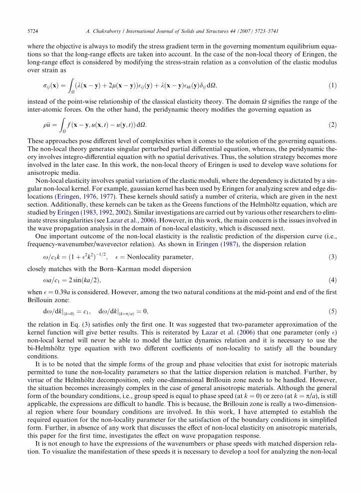
, m

Fig. 3. Escape frequency variation with non-locality parameter, �.


aðk; gÞx4 þ bðk; gÞx2 þ cðk; gÞ ¼ 0; ð27Þ

where the coefficients are

a ¼ 2�2q2k2 þ q2 þ �4q2k4 þ 2�2q2g2 þ �4q2g4 þ 2�4q2g2k2; ð28Þ

b ¼ �Q11g2�2qk2 � �2qg4Q66 � qQ22k2 � 2�2qQ66g

2k2 � Q66qk2

� �2qg2Q22k2 � Q66�2qk4 � Q11g

2q� Q11g4�2q� �2qQ22k4 � qQ66g

2; ð29Þ

c ¼ Q66Q22k4 þ Q11g2Q22k2 þ Q11g

4Q66 � g2Q212k2 � 2g2Q12Q66k2: ð30Þ

Solving Eq. (27) the expression of x is obtained, which in turn gives the expressions of the group speeds byappealing to the definition.

Figs. 4 and 5 show the group speeds in the Y(Cg,k) and X(Cg,g) direction, respectively. It is clear that athigher frequencies, local theory predicts both the modes as propagating (one at 1600 m/s and the other ataround 2600 m/s). On the other hand, non-local theory says that beyond the escape frequencies, Cg,k ceasesto exist and the contribution comes only from the other speed Cg,g. Even in the second case, there is a zonewhere both the modes are non-propagating, which in this case is between [xe1, 120 kHz]. The upper bound ofthis energy gap can easily be found from the expressions of the group speeds.

Similar kind of variation can be observed when Al-crystal is studied. Fig. 6 shows the wavenumber varia-tion where again the cut-off frequencies and escape frequencies are clearly visible. In the dispersion relations,Cg,k variation is similar to the GFRP. However, Cg,g variation suggests that unlike GFRP, there is no energygap for which both the modes are non-propagating.

Coming to the estimation of the non-locality parameter �, the 2D counterparts of the conditions given inEq. (5) are to be satisfied. Here, for simplicity, we concentrate only on the second condition, i.e., the groupspeeds are zero at the edge of the Brillouin zone, i.e., at k = ±p/a edge and g = ±p/a edge. Instead of directlysatisfying the condition, a simplified approach will be to satisfy

ox2=okjðk¼p=a;g¼p=aÞ ¼ 0; ox2=ogjðk¼p=a;g¼p=aÞ ¼ 0; ð31Þ

i.e., only at the vertex of the Wigner–Seitz cell in the first quadrant. Even this condition generates complicatedexpressions involving the material properties Qij and �. For example the first condition gives

Fig. 5. Group speed, Cg,g variation with frequency, g = 10, GFRP.

Local (2)

Local (1)

Fig. 4. Group speed, Cg,k variation with frequency, g = 10, GFRP.


2Q66Q22p2e2 � Q22r1a2 � Q66r1a2 � Q222p2e2 þ e2p2Q2

11

þ Q66Q22a2 � Q66Q11a2 þ Q11Q22a2 � 4Q12Q66a2 � 2Q266a2

� Q222a2 � 2Q2

12a2 � 2Q66Q11p2e2 � Q22p

2r1e2 þ e2p2r1Q11 ¼ 0; ð32Þ

where; r1 ¼ffiffiffiffiffiffiffiffiffiffiffiffiffiffiffiffiffiffiffiffiffiffiffiffiffiffiffiffiffiffiffiffiffiffiffiffiffiffiffiffiffiffiffiffiffiffiffiffiffiffiffiffiffiffiffiffiffiffiffiffiffiffiffiffiffiffiffiffiffiffiffiffiffiffiffiffiffiffiffiffiffiffiffiffiffiffiffiffiffiffiffiffiffiffi4Q2

66 þ Q222 � 2Q11Q22 þ Q2

11 þ 4Q212 þ 8Q12Q66

q;

which is an expression involving �2 and a2. Thus, it can readily be solved for � as

� ¼ pa

ffiffiffiffiND

r; ð33Þ

Fig. 6. Wavenumber variation with frequency, g = 10, Al-crystal.


where the numerator N and the denominator D are

N ¼ 4Q12Q66 þ ðQ22 þ Q66Þr1� Q11Q22 � Q66Q22 þ Q66Q11 þ 2Q212 þ 2Q2

66 þ Q222; ð34Þ

D ¼ ðQ11 � Q22ÞðQ11 � 2Q66 þ Q22 þ r1Þ; ð35Þ

and r1 is same as defined in Eq. (32). It is important to note that no solution exists when Q11 = Q22. Thisbrings out the lack of degeneracy of the system from the (initial) anisotropic to isotropic situation. In theisotropic case, the � value is independent of the material properties, (so is wave amplitude). However, inthe anisotropic case, � is material property dependent, which again reiterates the non-existence of the Helm-holtz decomposition.

For GFRP, with the material properties assumed for the wavenumber study, the � values obtained for thefour cases are as follows:

ox21=okjðk¼g¼p=aÞ ¼ 0; � ¼ 0:0568a

ox22=okjðk¼g¼p=aÞ ¼ 0; � ¼ j0:4276a

ox21=ogjðk¼g¼p=aÞ ¼ 0; � ¼ j0:3233a

ox22=ogjðk¼g¼p=aÞ ¼ 0; � ¼ 0:28556a:

Thus, there are two imaginary values which are to be discarded from the viewpoint of physical significance.The other two values are relevant in the sense that they can serve as the lower and upper bound for �. It isworth mentioning that the upper bound is close to the estimation of Kunin (1983). However, further investi-gation is necessary to fully understand the relevance of the values and justify the method.

Once the wavenumbers are known in terms of the frequency xn and wavenumber gm, the spectral elementscan be formulated for each n and m by following the procedure described below.

2.1. Spectral element for layered media

Once the four wavenumbers and wave amplitudes are known, the four partial waves can be constructed andthe displacement field can be written as a linear combination of the partial waves. Each partial wave is givenby


ai ¼ui

vi

� �¼

R1i

R2i

� �e�jkiy

sinðgmxÞcosðgmxÞ

� �e�jxnt; i ¼ 1; . . . ; 4; ð36Þ

and the total solution is

u ¼X4

i¼1

Ciai: ð37Þ

2.1.1. Finite layer element (FLE)

The solutions of u and v in the form of Eq. (37) is utilized to form the element dynamic stiffness matrix at xn

and gm. In the first step, the expressions of u and v are evaluated at the two edges of the layer, i.e., at y = 0 andL (see Fig. 1(b)). This generates four equations:

Uð0Þ ¼ u1nm; UðLÞ ¼ u2nm; V ð0Þ ¼ v1nm; V ðLÞ ¼ v2nm; ð38Þ
Thus, nodal displacements are related to the unknown constants by
fu1nmv1nmu2nmv2nmgT ¼ ½T1nm�fC1C2C3C4gT; ð39Þ

i.e.,

fugnm ¼ ½T1�nmfCgnm: ð40Þ
In the second step, the nodal tractions are to be evaluated at y = 0 and L and linked to the unknown constantsCi-s. To do that, the integral in Eq. (13) is to be evaluated assuming a valid kernel function a(r). Let us definethe local form of the stresses as
r11ðxÞr22ðxÞr12ðxÞ

8><>:

9>=>; ¼

Q11 Q12 0

Q12 Q22 0

0 0 Q66

264

375

e11ðxÞe22ðxÞe12ðxÞ

8><>:

9>=>;; ð41Þ

then the relation between the local and global forms of the stresses is (see Eringen, 1987)

tpq ¼ ð1þ �2r2Þrpq: ð42Þ
Based on the assumption of the displacement field the above relation becomes
tpq ¼ ½1� �2ðg2m þ k2

mnÞ�rpq ¼rpq

1þ �2ðg2m þ k2

mnÞ; ð43Þ

where kmn is any of the four wavenumbers at frequency xn and wavenumber gm and the last relation is possiblebecause �� 1. It is to be noted that Eq. (43) can also be obtained by integrating the kernel function (as shownin Artan and Altan, 2002). Following the same reference if a is assumed as

aðjx� x0jÞ ¼ 1

2p�2K0ð��1

ffiffiffiffiffiffiffiffiffiffiffiffiffiffiffiffiffiffiffiffiffiffiffiffiffiffiffiffiffiffiffiffiffiffiffiffiffiffiffiffiðx� x0Þ2 þ ðy� y0Þ2

qÞ; ð44Þ

where K0 is the modified Bessel function of the second kind, the integral to be evaluated is

1

2p�2

ZX

aðjx� x0jÞf ðx; x0Þdx0 ¼ f ðxÞ1þ �2ðg2

m þ k2mnÞ

; ð45Þ

where f ðxÞ ¼ sinðgmxÞcosðgmxÞ

� �� expð�jkmnyÞ and the expression of tpq is same as that of Eq. (43). The traction

boundary condition is given in terms of the non-local stresses as

T p ¼ tpqnq; ð46Þ
where nq is the direction cosine of the surface normals. For the layer element the edges are oriented in such away that nx = 0 and ny = �1. Thus, the expressions of the tractions are simplified to Tx = �txy and Ty = �tyy.
Using Eq. (43), edge tractions are related to the constants by

fTgnm ¼ ½S2�nmfCgnm; fTgnm ¼ f�txyð0Þ;�tyyð0Þ; txyðLÞ; tyyðLÞg: ð47Þ


Explicit forms of S2nm and T1nm are

T1 ¼

R11 R12 R13 R14

R21 R22 R23 R24

R11eð�jk1LÞ R12eð�jk2LÞ R13eðþjk1LÞ R14eðþjk2LÞ

R21eð�jk1LÞ R22eð�jk2LÞ R23eðþjk1LÞ R24eðþjk2LÞ

26664

37775; ð48Þ

S2ð1; pÞ ¼ �Q66ð�jR1pkp � gmR2pÞ=ð1þ �2ðg2m þ k2

pÞÞ;S2ð2; pÞ ¼ ðjQ22R2pkp � Q12gmR1pÞ=ð1þ �2ðg2

m þ k2pÞÞ;

S2ð3; pÞ ¼ Q66ð�jR1pkp � gmR2pÞeð�jkpLÞ=ð1þ �2ðg2m þ k2

pÞÞ;S2ð4; pÞ ¼ f�jQ22R2pkp þ Q12gmR1pgeð�jkpLÞ=ð1þ �2ðg2

m þ k2pÞÞ;

where p ranges from 1 to 4.Thus, the dynamic stiffness matrix becomes

½K�nm ¼ ½S2�nm½T1��1nm ; ð49Þ

which is of size 4 · 4 and having xn and gm as parameters. This matrix exactly represents the dynamics of anentire layer of any thickness L at frequency xn and horizontal wavenumber gm. Consequently, this small ma-trix acts as a substitute of the global stiffness matrix of a FE model, whose size, depending upon the thicknessof the layer, will be many order larger than the spectral element size.

2.1.2. Infinite layer element (ILE)

This element is formulated by considering only the forward moving wave components, which means noreflection will come back from the boundary. This element acts as a conduit to throw away energy fromthe system and is very effective in modeling infinite domain in the Y direction. This element is also used toimpose absorbing boundary conditions or to introduce maximum damping in the structure. The elementhas only one edge where displacements are to be measured and tractions are to be specified. The displacementfield for this element (at xn and gm) is

unm ¼ R11C1nme�jk1y þ R12C2nme�jk2y ; ð50Þ

vnm ¼ R21C1nme�jk1y þ R22C2nme�jk2y ; ð51Þ

where it is assumed that k1 and k2 are having positive real parts. Following the same procedure as before, dis-placement at node 1 (see Fig. 1(a)) can be related to the constants Ci,i = 1, . . ., 2 as

fugnm ¼ ½T1�nmfCgnm: ð52Þ

Similarly, tractions at node 1 can be related to the constants as

fT x1T y1gTnm ¼ ½S2�nmfC1nmC2nmgT

; i:e:; fTgnm ¼ ½S2�nmfCgnm: ð53Þ

Explicit forms of the matrix T1 and S2 are

T1ðILEÞ ¼ T1ðFLEÞ ð1 : 2; 1 : 2Þ; S2ðILEÞ ¼ S2ðFLEÞ ð1 : 2; 1 : 2Þ: ð54Þ

The dynamic stiffness for the infinite half space becomes

½K�nm ¼ ½S2�nm½T1��1nm ; ð55Þ

which is a 2 · 2 complex matrix.

2.2. Prescription of the boundary conditions

Essential boundary conditions are prescribed in the usual way as is done in the FEM, where simply thenodal displacements are arrested or released depending upon the nature of the boundary condition.


The applied tractions are to be prescribed at the edges, where it is assumed that the loading functions (for sym-metric distribution about the Y axis) can be written as

F ðx; y; tÞ ¼ dðy� yiÞXM

m¼1

am cosðgmxÞ ! XN�1

n¼0

f nejxnt

!; ð56Þ

where d denotes the Dirac delta function and yi is the Y coordinate of the edge where the load is applied (loadis applied at the node/edge). No variation of loading in the Y direction is allowed in this analysis, although theextension is straight-forward. The am is the mth Fourier cosine series coefficient of the spatial distributionfunction of the load and f n is the nth Fourier transform coefficient for the time-dependent part of the load.

There are two summations in the solution and two associated windows, one in time T and the other inspace, Lx. The discrete frequency xn and the wavenumber gm are related to these windows by the numberof data points considered, N and M, chosen for each summation, i.e., Figs. 7 and 8

xn ¼ 2pn=T ¼ 2pn=ðNDtÞ; gm ¼ 2pðm� 1Þ=Lx ¼ 2pðm� 1Þ=ðMDxÞ; ð57Þ

where Dt and Dx are the temporal and spatial sampling rate, respectively.

2.3. Computation of the Lamb wave modes

By definition, the Lamb waves are guided waves propagating in a free plate while the top and bottom sur-faces of the plate are stress-free. For isotropic materials, the Helmholtz decomposition based analysis in con-junction with the imposition of the stress-free boundary conditions directly generate the equations governingthe symmetric and anti-symmetric modes (see Fig. 9). However, in the general framework followed so far, wecan appeal directly to the discretized governing equation in the frequency-wavenumber domain, i.e.,½Kðgm;xnÞ�fug ¼ f0g. Thus, for non-trivial solution, the dynamic stiffness matrix of the FLE, ½Kðgm;xnÞ�should be singular, which is the required condition for obtaining the wavenumber gm given the frequency xn.

Thus, contrary to the general case where gm is independently varied like the frequency and computed fromthe second expression of Eq. (57), gm for the Lamb wave modes are calculated from the transcendental equa-tion detðKnmÞ ¼ 0. However, the speed of computation can be improved substantially if we work on the gen-eralized coordinates Ci-s as opposed to the nodal coordinates. In that case, the non-singularity conditionbecomes detðS2nmÞ ¼ 0. However, the boundary conditions are applied at �h/2, (as opposed to y = 0 and L

0 50 100 150 200 250 300–2000

–1000

0

1000

2000

3000

4000

5000

6000

7000

Frequency, [kHz]

ωk, [

m/s

] local (1)

local (2)

Fig. 7. Group speed, Cg,k variation with frequency, g = 10, Al-crystal.

Fig. 8. Group speed, Cg,g variation with frequency, g = 10, Al-crystal.

Fig. 9. Lamb wave modes: (a) symmetric and (b) anti-symmetric.


for the element stiffness matrix development) and the non-singularity condition is written in terms of a newmatrix Wnm, i.e., detðWnmÞ ¼ 0 where

W ð1; pÞ ¼ ð�jR1pkp � gmR2pÞjðþjkph=2Þ=½1þ �2ðg2m þ k2

pÞ�;W ð2; pÞ ¼ ðjQ22=Q12R2pkp � gmR1pÞeðþjkph=2Þ=½1þ �2ðg2

m þ k2pÞ�;

W ð3; pÞ ¼ ð�jR1pkp � gmR2pÞeð�jkph=2Þ=½1þ �2ðg2m þ k2

pÞ�;W ð4; pÞ ¼ f�jQ22=Q12R2pkp þ gmR1pgeð�jkph=2Þ=½1þ �2ðg2

m þ k2pÞ�;

where as before p ranges from 1 to 4. It is to be noted that kp is related to xn and gm by the spectrum relationEq. (23).

Once gm is calculated for a given xn and kp-s are obtained from Eq. (23), the wave amplitudes R can becomputed by the SVD method described before and the complete solution can be formed by utilizing Eq.(37). The modes of Lamb wave are generally plotted in terms of the phase velocity, which is defined ascmn = xn/gm(xn). It is worthy of mentioning that if the stiffness matrix of the ILE is used instead of FLE, thenthe modes of Rayleigh waves will be obtained.

3. Numerical analysis

This section describes the application of the developed spectral elements to bring out the salient features ofthe waves propagating in a medium with non-local elastic definitions as opposed to the classical local elasticity.


In the discussions of the wavenumber computation, two different regions in the spectrum relation are men-tioned. The region with frequencies lower than xe is referred as the sub-critical region and similarly the higherside as the super-critical region. These regions are of different importance in terms of the material response. Inthe sub-critical region, there is not much difference between the local and non-local theory predictions. Thus,the responses of the media will be more or less identical, especially when broad-band excitation is used. How-ever, in the super-critical region, totally different responses can be envisaged because of the difference in thetype of wavenumbers. The numerical studies bring out these predictions more graphically. Further, the effectof non-locality on the modes of Lamb waves (and in turn on the time domain response) is demonstrated.

3.1. Wave propagation in the sub/super-critical regions

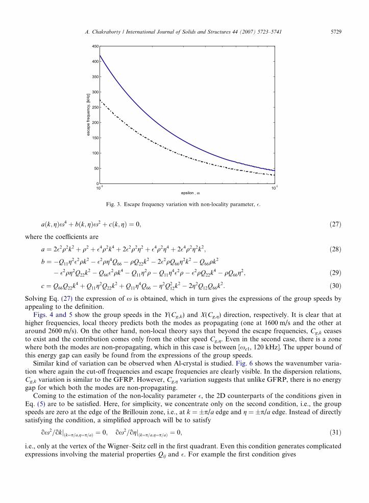
The first example explores the wave propagation in the sub-critical (below the minimum escape frequency)and the super-critical regions (above the maximum escape frequency) for a GFRP composite layered struc-ture. There are three different layers, each one 0.1 m thick. Although any layer thickness could have been cho-sen, this unusually large thickness is taken to have clear representation in the time domain response. The plystacking sequence for the layers are 0�, 90� and 0�, respectively. The material properties considered are as fol-lows: E1 = 144.48 GPa, E2 = E3 = 9.632 GPa, m23 = 0.3, m13 = 0.02, G12 = 4.128 GPa and q = 1389 kg/m3.Based on these material properties, and a non-locality parameter � = 0.004 m, the spectrum relation is solvedagain for 90� ply-angle and shown in Fig. 10. As the figure suggests, the sub-critical region is below 70 kHzand the super-critical region is above 110 kHz. Thus, the load of excitation should be in these regions tonumerically track the solutions.

The structure is fixed at the bottom and free at the top where modulated pulse loadings are applied. Twodifferent loadings are considered, one modulated at 40 kHz and the other modulated at 200 kHz. The spatialvariation for both the loading is same and shown in Fig. 11. As the figure suggests first 100 Fourier cosinemodes are sufficient to represent the load and thus for all subsequent analysis, M = 100 is considered. Theloads are applied in the Y direction and the Y velocity at the surface is measured at X = 0. It is to be notedthat according to the Fourier transform the X domain of the model is [�Lx/2,Lx/2]. All the non-local materialresponses are compared with the corresponding local theory based responses.

The velocity responses for the sub-critical excitation is shown in Fig. 12. The difference in the local and non-local theory based responses brings out the effect of the differences in the corresponding wavenumbers. It is

0 50 100 150 200 250 300 350 4000

100

200

300

400

500

600

700

800

900

1000

Frequency, [kHz]

Wav

enum

ber,

[m–1

]

Fig. 10. Position of excitation in the spectrum relation.

Fig. 11. Fourier cosine coefficients of the load: inset shows the spatial distribution.

0 0.2 0.4 0.6 0.8 1 1.2 1.4 1.6 1.8 2

x 10–3

–4

–3

–2

–1

0

1

2

3

4x 10

–8

Y–v

eloc

ity, [

m/s

]

Time, [s]

ε = 0.004 m

LocalNon–local

Fig. 12. Y-velocity response for the sub-critical excitation.


evident from Figs. 4 and 5 that the group speeds are drastically different for the two different theories. This ismanifested in Fig. 12, where the reflections from the ply-interfaces and the fixed boundary do not appear at thesame time for the two theories. Thus, there are extra waveforms (e.g., one at 1.1 ms) for the non-local theorywhich is absent in the case of local theory based response. Further, the local theory based response has smalleramplitudes compared to the other response.

Next, we apply the super-critical frequency loading in the Y direction and measure the same entity at thesame point on the surface. The responses based on the local and non-local theories are shown in Fig. 13.

0 0.1 0.2 0.3 0.4 0.5 0.6 0.7 0.8 0.9 1

x 10–3

–4

–2

0

2

4

6

8

10x 10

–8

Y–v

eloc

ity, [

m/s

]

Time, [s]

ε = 0.004 m

Non–local

Local

Fig. 13. Y-velocity response for the super-critical excitation.


As the figure suggests, local theory shows both the incident pulse (starts at 0.1 ms) and the reflected pulse (thesecond waveform), whereas, the non-local theory does not predict any reflected waveform. This is because, inthe super-critical zone, at this particular frequency, non-local theory predicts both the group speeds as zero(see Figs. 4 and 5). Thus, the present form of the non-local theory suggests that at very high frequencies(beyond the escape frequency) the damping due to material non-locality will suppress all responses. Thismay very well suggest that the non-local theory should be used with caution, especially beyond the escapefrequency.

3.2. Propagation of Lamb wave

A uni-directional laminae of 2 mm thickness is considered for the study of propagating Lamb wave modeswhere studying the effect of non-locality is the objective. Analyses are performed for two different fibre-direc-tions, 0� and 90�. Material properties of the composites are as taken before and the non-locality parameter� = 1 · 10�4 m. Because of the complex expressions, the dispersion relation (relation between cp = x/g andx) is usually left in the form of a determinant equal to zero. Solutions for this kind of implicit equationrequires special treatment. The solution, moreover, is multi-valued, unbounded and complex (although thereal part is only of interest). One way of solving the equation is to treat it as a non-linear optimization problembased on non-linear least square method. Here, MATLAB� function fsolve is used and the default optionfor medium scale optimization – the trust-region method is adopted, which is a variant of the Powell’s doglegmethod.

Apart from the choice of algorithm there are other subtle issues in root capturing for the solution of wave-numbers as the solutions are complicated in nature. Moreover, except the first one or two modes, all the otherroots escape to infinity at low frequency. For isotropic materials, these critical frequencies are known belowwhich the phase speed is infinite. However, no expressions can be found for anisotropic materials and most ofthe times, the modes (solutions) should be tracked backward, i.e., from higher frequency to lower frequency.In general two strategies are essential to capture all the modes within a given frequency band. Initially, thewhole region should be swept for different values of the initial guess, where the initial guess should remainconstant for the whole range of frequency. This sweeping opens up all the modes in that region, although theyare not completely traced. Subsequently, each individual mode should be followed to the end of the domain or


to a pre-set high value of the solution. For this case, the initial guess should be changed for each frequency tothe solution of the previous frequency step. Also, sometimes it is necessary to reduce the frequency step in thevicinity of high gradient of the modes.

The Lamb wave modes for 0� ply-angle is shown in Fig. 14. The symmetric and anti-symmetric modes arepointed by the letters s and a. For the local theory, the first anti-symmetric mode, a0, converges to a value of1719 m/s in a range of 1 MHz mm, where the other modes converge later. This is the Rayleigh surface wavespeed (cR) for 0� ply. The first symmetric mode (s0) starts at around 10,000 m/s and after a sudden drop at1.3 MHz mm converges to cR. The difference between the local and non-local theory becomes pronouncedafter 1.5 MHz mm. All the modes predicted by the non-local theory are shifted to the left and the higher ordermodes are affected more. For the non-local theory, the mode a0 does not converge to any value but decreasesafter 2 MHz mm and other modes also follow the same trait. Thus, at higher frequencies, lower order modesbecome dispersive and eventually cease to exist. For example, for a frequency-thickness value of 8 MHz mm, itis most unlikely that the first four modes will be present, whereas, for the local theory these modes will stillcontribute. Thus, the non-local theory at high frequencies will have less participation from the propagatingmodes. Further, the Rayleigh wave speed is shown to be frequency-dependent (unlike the classical elasticitycase) and the wave eventually disappears as the energy gap region is approached.

Similarly, for 90� ply-angle the Lamb wave modes are plotted in Fig. 15 and the local/non-local theorybased predictions are compared. The figure is characterized by a large number of modal participation, espe-cially for the non-local theory. However, the modes are all decreasing steadily which says that beyond a certainfrequency, these modes will be completely evanescent. The effect of increasing � is shown for the mode a0. Fur-ther, at lower frequency-thickness non-local theory brings higher number of modes inside the window of inter-est. The dispersive nature of the Rayleigh wave is also evident in this case.

Once the Lamb modes are generated they are substituted back into the frequency loop to create the fre-quency domain solution of the Lamb wave propagation, which through IFFT produces the time domain sig-nal. As the Lamb modes are generated first, they need to be stored separately. To this end data are collectedfrom the generated modes at several discrete points in the whole range of frequency. Next, a cubic spline inter-polation is performed for a very fine frequency step within the same range. While generating the time domaindata, interpolation is performed from these finely graded data to get the phase speed (hence, g). The timedomain signatures are not shown here although they resemble the results shown in the previous work

Fig. 14. Lamb wave modes for 0� ply-angle, � = 1.0 · 10�4 m.

Fig. 15. Lamb wave modes for 90� ply-angle, � = 1.0 · 10�4 m.


(Chakraborty and Gopalakrishnan, 2004). For non-local theory the signature differs only in the time ofappearance.

4. Conclusion

Spectral Finite Element method is employed to understand the effect of non-local elasticity on the wavepropagation response of general anisotropic materials, in particular, fiber reinforced composites. Two differentfrequency regions are identified, where non-locality plays different types of role. In the lower frequency side,the modes maintain their main characteristics (propagating or evanescent) and the dispersion relations are per-turbed slightly. Thus, only the time of arrival of responses differ between the classical and non-local elasticity.In the second (high-frequency) region, modes are completely suppressed by the non-locality and thus, at cer-tain frequency there may not be any propagating mode at all, i.e., non-locality at high frequency works as adamping. Similar effect can be observed for the Lamb wave modes. At high frequencies, all the modes becomedispersive in the case of non-local elasticity, which are otherwise non-dispersive. Thus, for non-local elasticity,with increasing frequency, modal participation decreases.

Estimation of the non-local parameter by comparing the lattice dynamics based dispersion relation bringsout several issues. In general, it seems impossible to match all the boundary conditions at the edges of the Wig-ner–Seitz cell at two-dimension. The attempt to satisfy the boundary condition at one vertex of the cell pro-duces two values of the parameter �. The significance of these values is still not understood. It is postulatedthat they can serve as the lower and upper bound for the values the parameter can take. Further researchin this regard is necessary to fully understand the relation between lattice models and their continuumcounterparts.

References

Artan, R., Altan, B., 2002. Propagation of sv waves in a periodically layered media in nonlocal elasticity. Int. J. Solid. Struct. 39, 5927–5944.

Chakraborty, A., 2007. Shell element based model for wave propagation analysis in multi-wall carbon nanotube. Int. J. Solid. Struct. 44(5), 1628–1642.

Chakraborty, A., Gopalakrishnan, S., 2004. A spectrally formulated finite element for wave propagation analysis in layered compositemedia. Int. J. Solid. Struct. 41 (18–19), 5155–5183.


Chakraborty, A., Gopalakrishnan, S., 2005. A spectrally formulated plate element for wave propagation analysis in anisotropic material.Comput. Meth. Appl. Mech. Engg. 194 (42–44), 4425–4446.

Chakraborty, A., Gopalakrishnan, S., 2006. A spectral finite element model for wave propagation analysis in laminated composite plate. J.Vibr. Ac. 128 (4), 477–488.

Chakraborty, A., Sivakumar, M., Gopalakrishnan, S., 2006. Spectral element based model for wave propagation analysis in multi-wallcarbon nanotubes. Int. J. Solid. Struct. 43 (2), 279–294.

Doyle, J.F., 1997. Wave Propagation in Structures. Springer, Berlin.Eringen, A., 1976. Edge dislocation in nonlocal elasticity. Int. J. Eng. Sci. 10, 233–248.Eringen, A., 1977. Screw dislocation in nonlocal elasticity. J. Phys. D: Appl. Phys. 10, 671–678.Eringen, A., 1983. On differential equation of nonlocal elasticity and solutions of screw dislocation and surface waves. J. Appl. Phys. 54,

4703–4710.Eringen, A., 1987. Theory of nonlocal elasticity and some applications. Res. Mech. 21, 313–342.Eringen, A., 1992. Vistas of nonlocal continuum physics. Int. J. Eng. Sci. 30, 1551–1565.Eringen, A., 2002. Nonlocal Continuum Field Theories. Springer, New York.Kunin, I.A., 1983. Elastic Media With Microstructure II: Three-dimensional Models. Springer, Berlin.Lazar, M., Maugin, G., Aifantis, E.C., 2006. On the theory of nonlocal elasticity of bi-helmholtz type and some applications. Int. J. Solid.

Struct. 43, 1404–1421.Love, A.E.H., 1944. A Treatise on Mathematical Theory of Elasticity. Dover, New York.Silling, S.A., 2000. Reformulation of elasticity theory for discontinuities and long range forces. J. Mech. Phys. Solid. 48, 175–209.

Documents

Wave propagation in anisotropic media with non-local ... · Wave propagation in anisotropic media with non ... local elasticity on the wave propagation ... analysis in anisotropic