Watertight As-Built Architectural Floor Plans Generated from Laser RangeData

Eric Turner and Avideh ZakhorU. C. Berkeley

Department of Electrical Engineering and Computer ScienceBerkeley, CA 94720

elturner@eecs.berkeley.edu, avz@eecs.berkeley.edu

Abstract

This paper proposes an algorithm that generates as-builtarchitectural floor plans by separating the floors of the Li-DAR scan of a building, selecting a representative samplingof wall scans for each floor, and triangulating these sam-plings to develop a watertight representation of the wallsfor each of the scanned areas. Curves and straight linesegments are fit to these walls, in order to mitigate anyregistration errors from the original scans. This methodis not dependent on the scanning system and can success-fully process noisy scans with non-zero registration error.Most of the processing is performed after a dramatic di-mensionality reduction, yielding a scalable approach. Wedemonstrate the effectiveness of our approach on a three-story point cloud from a commercial building as well as onthe lobby and hallways of a hotel.

1. Introduction

The use of laser scanning technology is becoming a vitalcomponent of building construction and maintenance. Dur-ing construction, laser scanning can be used to record theas-built locations of HVAC and plumbing systems beforedrywall is installed. In existing buildings, blueprints areoften outdated or missing, especially after several remod-elings. In this paper we describe an approach to automati-cally generate a floor plan for the interior environment of abuilding using laser scan data. This floor plan is meant toaccurately indicate the positions of walls within an area ofinterest in the building.

The point clouds generated from these scans representhuge amounts of data that may contain noise or missinggaps. There may exist excess clutter such as furniture orother non-building objects. An existing and more usableformat in the architectural field is a 2D floor plan for thezones of interest. The ability to separate these building el-

ements from the rest of the point scans and to generate acoherent floor plan can potentially enhance semantic under-standing of a point cloud representing an architectural envi-ronment.

Accurate floor plans can also be used to generate full3D models of a building. The input floor plans of thesemodeling systems should not contain temporary objects orclutter. The techniques described in [10, 13] spend signifi-cant effort to discover walls and shapes in a rasterized floorplan. Having a plan that is already represented by paramet-ric curves and lines, such as the output of the approach to bedescribed in this paper, can facilitate modeling algorithmsthat incorporate 2D information [3, 4, 10, 13]. The result-ing 3D models can be used for virtual reality or in-buildingnavigation purposes. Both these 3D models as well as 2Dfloor-plans can be used to generate semantic Building In-formation Models (BIM), which can be used for buildingmaintenance and energy-efficiency analysis [15].

2. Background

Point cloud scans of building interiors can be captured ina variety of ways. With static scanning, a stationary scan-ner is manually placed at a finite number of locations inthe building to collect scans. In mobile scanning, a singlescanning system collects data continuously while movingthrough the environment. In both cases, scans taken fromdifferent locations must be registered against each other, sothat all scan points are represented in the same coordinateframe. Any errors in this registration process can causeerrors in the resultant point cloud. Applications that ana-lyze this point cloud must take these potential errors intoaccount.

An architectural floor plan is defined to represent a sub-set of the interior walls and hallways of a building. It isoften preferred that floor plans contain semantic informa-tion, such as the swing direction of doorways or restroomlabels. These features are not a requirement and the pro-

1

cessing required to produce them is beyond the scope ofthis paper. The shape and configuration of wall placementsin floor plans are not arbitrary, but adhere to common prac-tices and patterns. Walls customarily are simple geomet-ric shapes, such as straight line segments or smooth curves[15]. The placement of walls with respect to one anotheris also methodical. Many building floor plan designs uti-lize patterns and regularity to reduce the complexity of thedesign and construction process [6]. The symmetric andrepeating pattern common in many buildings can be usedto reduce noise in an estimated model. Since the techniquesproposed in this paper are meant to be dispatched on subsetsof a building’s interior, the patterns across an entire buildingcannot always be utilized.

3D modeling of building environments is a well-studiedfield. Aerial and terrestrial laser scanning of urban envi-ronments has yielded accurate, detailed models of externalarchitectures [14, 17]. Since exterior scans typically passthrough windows and other openings in a building facade,they can be used to create a sparse representation of the in-terior floor plan [7].

Interior scanning has traditionally been used for roboticnavigation in indoor environments. The rough locations ofwalls are necessary to avoid collisions. Generating floorplans for modeling, however, requires a much higher de-gree of precision [12]. Given these antecedent studies, tech-niques have been developed using a single horizontal scan-ner collecting about the yaw direction [16]. Constructingfull 3D scans allows for more sophisticated means of iden-tifying walls from other obstacles in a building. In this sce-nario, one can compute a top-down 2D histogram of pointdensities across the x-y plane [12]. Areas with high densityare considered likely to be wall locations. While clutter ismitigated by being less represented in the histogram thanwalls, no direct measures are taken to remove outlier sam-ples before line-fitting. Further, each story of a buildingmust be processed separately.

Previous approaches to floor plan modeling typically as-sume walls are well-fitted by straight line segments andwhether these fitted models are watertight is not guaranteed[11, 12, 16]. Many architectural designs incorporate curvedfeatures, which would not be modeled accurately by theseapproaches. The absence of any water-tightness guaranteerequires extensive post-processing to be devoted to remov-ing disconnected and outlier segments that are interpretedas noise.

This paper presents a means of generating a floor planthat fits both curves and straight segments with walls thatare guaranteed to be watertight. In Section 3 we describeour approach. Sections 4 and 5 include results and conclu-sions.

3. Proposed ApproachGiven a point cloud representing a subset of the interior

of a building that can cover multiple stories, we proposea three-step process to generate a watertight floor plan foreach story in the point cloud by fitting line segments andcurves to model features. First, we extract wall samplelocations for each story. This process is done using a 2Dprojection and density analysis, in a similar manner as dis-cussed in [12]. The output is a subset of samples that arerepresentative of each wall on each story, as discussed inSections 3.1 and 3.2. Second, the Delaunay Triangulationof these samples is computed and each triangle is labeled as“internal” or “external” using a 2D version of the Eigencrustalgorithm [9]. This process is discussed in Section 3.3. Theedges that border these two labels are output as wall loca-tions, as detailed in Section 3.4. Thirdly, noise reduction isachieved by fitting these facets to line segments and curvedcomponents using Random Sample Consensus (RANSAC)[5], as discussed in Section 3.5.

3.1. Finding Wall Samples

Given a 3D input point set, P , we wish to generate afloor plan for each story represented. The coordinate sys-tem is defined so that the z-component represents height.First, we compute how many stories are present in P andpartition P into separate point sets P0, P1, ..., Pf for eachlevel by height, as shown in Figure 1. A histogram is calcu-lated for the distribution of the heights of all points p ∈ P .Next, we determine which bins of this histogram representthe locations of floors and ceilings. We only consider binsthat are local maxima and contain the highest counts. Thebins with the highest counts are found by sorting the binsby size in descending order and keeping the bins that ap-pear before the greatest discontinuity. This step chooses themost densely populated bins as potential floor and ceilinglocations. The bin with the lowest z-elevation that satisfiesthese requirements is assumed to be the floor of the firststory. The lowest floor/ceiling bin that is at least a mini-mum wall height threshold, typically taken to be∼2 meters,above the current floor bin is considered the ceiling bin forthat floor. The next highest floor/ceiling bin is taken to bethe floor height of the next story. This procedure contin-ues for all stories. A partition level is taken to be halfwaybetween the ceiling of one story and the floor of the nextstory. These levels partition the point set into f separatestories P0 ∪ P1 ∪ ... ∪ Pf−1 = P .

For each story k, we wish to determine what subset ofpoints in Pk represent walls. Our goal is to find these walllocations with a sparse sampling of points Sk ⊆ Pk. Bydefining a grid along the x-y plane, we can find coordinatelocations that are likely to represent walls. The width ofeach grid cell is the sampling distance ds, which should besmaller than the minimum feature size expected in a floor

(a) (b)

Figure 1. A point set P , shown in (a), is separated into three storiesP0, P1, and P2 based on a histogram analysis of point heights, asshown in (b).

Figure 2. A point set Pk (small dots in blue) is partitioned by agrid in the x-y plane (lines in black). For each grid cell, a neigh-borhood of points (medium dots in red) is computed and the me-dian position of the points (large dot in green) is taken as a wallsample. The normal of this neighborhood (vector in dark green) iscomputed using PCA.

plan. A typical value for this parameter is 5 cm. This gridpartitions Pk laterally. For a grid cell g, let the neighbor-hood set Ng be the subset of points of Pk that are within ahorizontal distance of ds from the center of g, as shown inFigure 2. Thus a given point can be in the neighborhood ofmultiple grid cells.

We perform the following checks on Ng to determinewhether this neighborhood represents a portion of a wall.The first assertion is that a wall must be densely sampled,so if |Ng| is less than a threshold, it is rejected. Typicallya threshold of |Ng| ≥ 50 points is sufficient. The secondcheck is to verify the height of a wall. The vertical supportof Ng must be at least the minimum wall height thresholdmentioned earlier. We wish to verify that the distribution ofpoints is uniform vertically, which signifies that a flat sur-face was captured. For this uniformity check, we computethe histogram of the heights of Ng with 16 bins and enforcethat at least 12 of these must be non-empty. Additionally,

Figure 3. Average filtering reduces occurrence of registration er-rors exposed in wall sampling.

at least three of the highest four bins must be non-empty,which ensures a neighborhood extends all the way to theceiling. If these requirements are fulfilled, g is said to repre-sent a wall. The median horizontal position for the elementsof Ng is computed. If this median lies within the bounds ofg, then it is taken as a “wall sample” for g.

The normal vector for this wall sample is calculated us-ing Principal Components Analysis (PCA) [8]. Let C be the2×2 covariance matrix of the x-y positions of the elementsof Ng and e1, e2 be the eigenvectors of C with correspond-ing eigenvalues λ1, λ2. Let λ1 ≤ λ2. The normal vector ischosen to be ~n = e1, as shown in Figure 2. The confidenceof this normal estimate is computed as c = 1− 2λ1

λ1+λ2. If c

is less than 0.15, then the neighborhood points are not well-aligned and rejected as the location for a wall.

If pose information for the scanner is known for eachpoint, this normal vector’s direction may be flipped to guar-antee that it points towards the laser scanner. Any wall sam-ples captured far away from the scanner are thrown away asoutliers. This distance is typically 5-10 meters. If a featurewas not scanned within this distance, it was only partiallycaptured and cannot be accurately represented. Performingthe above operation for all grid cells results in a set of wallsample points Sk ⊆ Pk.

3.2. Smoothing Wall Samples

A crucial step in generating a point cloud is to registerthe poses of separate scan positions to a common coordinatesystem. Any error in this process may result in duplicateinstances of a scanned wall with slight misalignments. Eachinstance of a wall may appear in Sk and if the registrationerror is significant smoothing may be required to force thesewall instances to become aligned.

For a given sample s ∈ Sk with normal vector ~n, itssmoothing set is a subset of Sk. The position of s is trans-lated to be the mean position of this smoothing set. Thesmoothing set contains all samples that are (a) within somesmoothing distance of s along the±~n direction, (b) no morethan 3ds away from s in the direction orthogonal to ~n, and

Figure 4. The angles of intersection between two triangles u andv, which share the edge s1s2. These values are used in computingweights between triangle pairs.

(c) whose normals are aligned to within π8 radians of ~n. The

smoothing distance must be less than the minimum allow-able spacing between parallel walls, but at least as large asthe expected registration error. This step is not necessaryif registration error is smaller than ds. An example of thissmoothing process is shown in Figure 3.

3.3. Labeling Triangulation of Wall Samples

We wish to determine the topology of the 2D sample setSk for each story k ∈ {0, 1, ..., f − 1}. This task is accom-plished using a 2D variant of the Eigencrust algorithm [9].This will partition 2D space into regions labeled “inside”and “outside” and export the borders between these regions.This method guarantees that these borders form the faces ofa 2D simplicial complex, which will be watertight. Eigen-crust has been shown to be more robust to outlier samplesthan similar algorithms, such as Powercrust [9, 1].

The Eigencrust algorithm first computes the 2D Delau-nay Triangulation, T , for the sample set Sk plus four bound-ing box corners. Eigencrust constructs a sparse graph wherethe nodes represent triangles and edges are placed betweenthe nodes with weights corresponding to the relative geom-etry of the triangles. Edges with positive weights indicatethat triangles should have the same labeling, while negativeweights indicate that the triangles connected should be la-beled oppositely. Generalized eigensystems are solved inorder to determine the best triangle labelings to fit theseconnections. For our 2D varient of Eigencrust, we keep thesame criteria for placing edge weights as in [9], but mod-ify the negative edge weight values. As compared to [9],we have additional information of normal vectors for eachsample location. If a negative edge is placed between twotriangles u and v, we use the weighting:

wu,v = −e4+4cosφ+2sinθ1+2sinθ2 (1)

where these parameters are shown in Figure 4. The valueφ is defined as the angle at which the circumcircles of u andv intersect. The intersection of the triangles u and v is aline segment whose endpoints are samples s1 and s2, which

Figure 5. An example triangulation of wall samples. Each triangleis denoted as “inside” (yellow) or “outside” (green).

have normal vectors ~n1 and ~n2 respectively. The value θ1

is defined to be the angle between ~n1 and s1s2, and θ2 isdefined as the angle between ~n2 and s1s2. This weight isdefined to have a large magnitude when both the normalvectors are perpendicular to the line s1s2, which is a strongindication of a wall in the original point cloud Pk.

We can constrain some triangles to be interior or exteriorbased on a priori information. The label “inside” refers tolocations of open area within a building where a person canexist. The term “outside” refers to all other areas, whichinclude both the exterior of the building as well as the ar-eas inside walls or other solid spaces. We can immediatelyforce the label of “outside” to any triangles connected tothe bounding box corner vertices. If the pose informationfor the scanner is available, we can force the label of “in-side” to a subset of triangles. First, we investigate whetherthe 2D line-of-sight from a scanner pose to a scan samplecrosses triangles. If the center 50% of this laser travel dis-tance crosses a triangle, that triangle is intersected by thatscan line. If a triangle is intersected by 10 or more scanlines, it is assumed to be “inside”. Additionally, all trian-gles that contain a pose position of a scanner are marked asinterior. If a mobile scanning system is used, then the pathtraversed by that system can also be used to mark interiortriangles. Each pair of adjacent pose positions represents aline segment in 2D space. If both of these poses contributedscans to the wall sample set Sk, then any triangles that areintersected by this line segment are also constrained to beinterior.

The remaining triangles are labeled inside or outside bysolving generalized eigenvalue systems that minimizes thetotal positive edge weights that connect oppositely labeledtriangles and negative edge weights that connect triangleswith the same labeling [9].

3.4. Forming Floor Plan Boundary Edges

We have found the following post-processing clean-uptechniques useful for increasing the quality of the outputmodel. First, we represent this topology of triangles as a

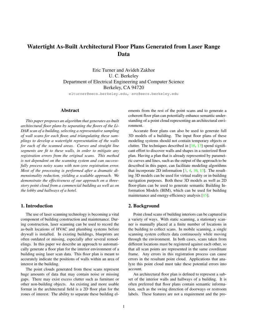
(a) (b)Figure 6. Original triangulation labeling (a) is cleaned by remov-ing small unions and sharp protrusions (b).

set of unions. Any subset of triangles with the same labelthat forms a connected component is represented as a sin-gle union using the Union-Find algorithm [2]. Unions thatare composed of a small number of triangles are most likelymislabeled, since the smallest building features should stillbe sufficiently sampled. The appropriate cut-off value de-pends on the value of ds used to form samples, but a valueof 30 triangles is typically used. All inside unions that havefewer than this many triangles are relabeled as outside. Theset of unions is recomputed and then all outside unions thatmeet this criterion are relabeled as inside. Another post-processing smoothing process is to remove jagged edgesfrom the boundaries between labelings. Every triangle hasthree neighboring triangles, each sharing one of its edges.If a triangle t ∈ T has only one neighbor that shares thesame labeling and that neighbor is connected to t’s shortestedge, then t is considered to be a protrusion. It is unlikelyfor building geometry to be correctly represented by such aprotrusion, so all protrusions labeled as inside are relabeledas outside. After this relabeling, all outside protrusions arefound and relabeled as inside. An example of this process-ing is shown in Figure 6.

The set of edges in T that are shared by an “inside” trian-gle and an “outside” triangle are exported as boundary edgeset, B. Each element in B is a line segment, which in totalconstitute a water-tight floor plan of the scanned area.

3.5. Fitting Edges With Lines and Curves

Since there may exist areas in the building geometry thatare insufficiently scanned or errors incurred during process-ing, it is important to utilize common architectural patternsto reduce these errors. Additionally, applications may re-quire a floor plan to be composed of parametric lines andcurves.

Local model-fitting approaches such as region growingare sub-optimal because unconnected architectural featuresmay use the same geometric model. For example, the backwalls in a row of offices may lie on the same plane, eventhough they are in different rooms. Since we need to fit bothcurves and straight lines simultaneously, a reasonable tech-nique for this situation is one that is non-local and flexible,

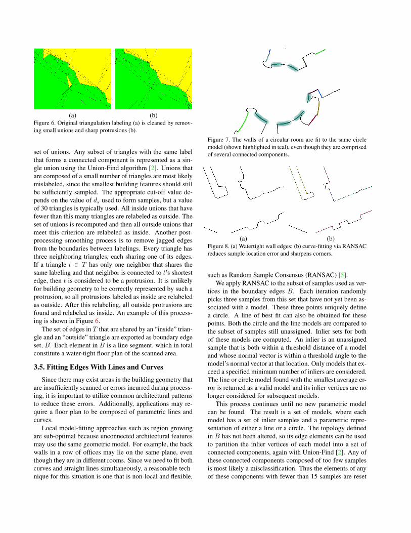
Figure 7. The walls of a circular room are fit to the same circlemodel (shown highlighted in teal), even though they are comprisedof several connected components.

(a) (b)Figure 8. (a) Watertight wall edges; (b) curve-fitting via RANSACreduces sample location error and sharpens corners.

such as Random Sample Consensus (RANSAC) [5].We apply RANSAC to the subset of samples used as ver-

tices in the boundary edges B. Each iteration randomlypicks three samples from this set that have not yet been as-sociated with a model. These three points uniquely definea circle. A line of best fit can also be obtained for thesepoints. Both the circle and the line models are compared tothe subset of samples still unassigned. Inlier sets for bothof these models are computed. An inlier is an unassignedsample that is both within a threshold distance of a modeland whose normal vector is within a threshold angle to themodel’s normal vector at that location. Only models that ex-ceed a specified minimum number of inliers are considered.The line or circle model found with the smallest average er-ror is returned as a valid model and its inlier vertices are nolonger considered for subsequent models.

This process continues until no new parametric modelcan be found. The result is a set of models, where eachmodel has a set of inlier samples and a parametric repre-sentation of either a line or a circle. The topology definedin B has not been altered, so its edge elements can be usedto partition the inlier vertices of each model into a set ofconnected components, again with Union-Find [2]. Any ofthese connected components composed of too few samplesis most likely a misclassification. Thus the elements of anyof these components with fewer than 15 samples are reset

to not be associated with any model. Additionally, we wishto encourage models to extend along the edges defined inB. If an unassigned sample is within 15 edge hops to sam-ples belonging to a model, that sample is associated withthe closest model. These two steps encourages outlier sam-ples to belong to models that are topologically close. Thesesteps also help grow models be adjacent, which encouragessharp corners.

Once the revised parametric models and their respectiveinliers are computed, the inlier samples and edges in B arereplaced by edges that conform exactly to their models’ lo-cations. This process reduces the overall number of samplesand removes small perturbation errors from the floor plan.Figure 7 demonstrates the results of this process, which fitsa circle to the walls of a round room with several entrances.Figure 8 shows how this process can also be applied tostraight walls.

4. ResultsOur approach can be applied to either static or mobile

scan systems and to point sets representing one or more sto-ries. Examples of these processes are shown in Figures 9,10, and 11.

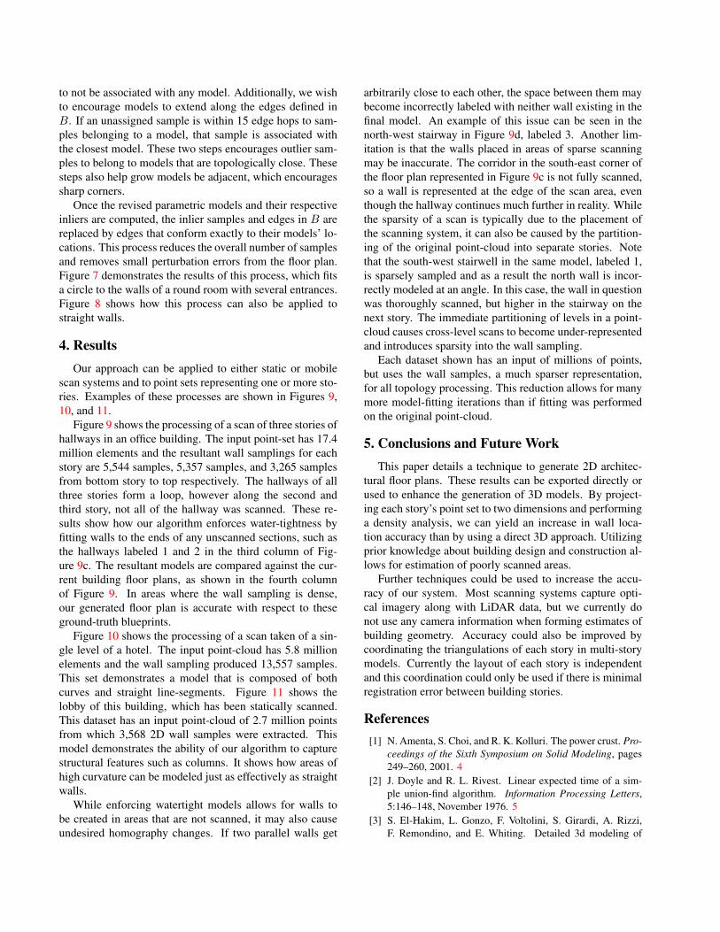
Figure 9 shows the processing of a scan of three stories ofhallways in an office building. The input point-set has 17.4million elements and the resultant wall samplings for eachstory are 5,544 samples, 5,357 samples, and 3,265 samplesfrom bottom story to top respectively. The hallways of allthree stories form a loop, however along the second andthird story, not all of the hallway was scanned. These re-sults show how our algorithm enforces water-tightness byfitting walls to the ends of any unscanned sections, such asthe hallways labeled 1 and 2 in the third column of Fig-ure 9c. The resultant models are compared against the cur-rent building floor plans, as shown in the fourth columnof Figure 9. In areas where the wall sampling is dense,our generated floor plan is accurate with respect to theseground-truth blueprints.

Figure 10 shows the processing of a scan taken of a sin-gle level of a hotel. The input point-cloud has 5.8 millionelements and the wall sampling produced 13,557 samples.This set demonstrates a model that is composed of bothcurves and straight line-segments. Figure 11 shows thelobby of this building, which has been statically scanned.This dataset has an input point-cloud of 2.7 million pointsfrom which 3,568 2D wall samples were extracted. Thismodel demonstrates the ability of our algorithm to capturestructural features such as columns. It shows how areas ofhigh curvature can be modeled just as effectively as straightwalls.

While enforcing watertight models allows for walls tobe created in areas that are not scanned, it may also causeundesired homography changes. If two parallel walls get

arbitrarily close to each other, the space between them maybecome incorrectly labeled with neither wall existing in thefinal model. An example of this issue can be seen in thenorth-west stairway in Figure 9d, labeled 3. Another lim-itation is that the walls placed in areas of sparse scanningmay be inaccurate. The corridor in the south-east corner ofthe floor plan represented in Figure 9c is not fully scanned,so a wall is represented at the edge of the scan area, eventhough the hallway continues much further in reality. Whilethe sparsity of a scan is typically due to the placement ofthe scanning system, it can also be caused by the partition-ing of the original point-cloud into separate stories. Notethat the south-west stairwell in the same model, labeled 1,is sparsely sampled and as a result the north wall is incor-rectly modeled at an angle. In this case, the wall in questionwas thoroughly scanned, but higher in the stairway on thenext story. The immediate partitioning of levels in a point-cloud causes cross-level scans to become under-representedand introduces sparsity into the wall sampling.

Each dataset shown has an input of millions of points,but uses the wall samples, a much sparser representation,for all topology processing. This reduction allows for manymore model-fitting iterations than if fitting was performedon the original point-cloud.

5. Conclusions and Future WorkThis paper details a technique to generate 2D architec-

tural floor plans. These results can be exported directly orused to enhance the generation of 3D models. By project-ing each story’s point set to two dimensions and performinga density analysis, we can yield an increase in wall loca-tion accuracy than by using a direct 3D approach. Utilizingprior knowledge about building design and construction al-lows for estimation of poorly scanned areas.

Further techniques could be used to increase the accu-racy of our system. Most scanning systems capture opti-cal imagery along with LiDAR data, but we currently donot use any camera information when forming estimates ofbuilding geometry. Accuracy could also be improved bycoordinating the triangulations of each story in multi-storymodels. Currently the layout of each story is independentand this coordination could only be used if there is minimalregistration error between building stories.

References[1] N. Amenta, S. Choi, and R. K. Kolluri. The power crust. Pro-

ceedings of the Sixth Symposium on Solid Modeling, pages249–260, 2001. 4

[2] J. Doyle and R. L. Rivest. Linear expected time of a sim-ple union-find algorithm. Information Processing Letters,5:146–148, November 1976. 5

[3] S. El-Hakim, L. Gonzo, F. Voltolini, S. Girardi, A. Rizzi,F. Remondino, and E. Whiting. Detailed 3d modeling of

(a)

(b)

(c)

(d)

Figure 9. (a) Full point cloud for three-story model, taken with mobile scanning system; (b-d) Processing of each story, with (left to right)wall sample locations, triangulation labeling, watertight curve-fit model, and comparison against ground-truth blueprints.

castles. International Journal of Architectural Computing,5(2):200–220, June 2007. 1

[4] S. El-Hakim, E. Whiting, L. Gonzo, and S. Girardi. 3-d re-construction of complex architectures from multiple data. 3D

Virtual Reconstruction and Visualization of Complex Archi-tectures, August 2005. 1

[5] M. A. Fischler and R. C. Bolles. Random sample consen-sus: A paradigm for model fitting with applications to image

(a) (b)

Figure 10. Hallway of hotel, captured with mobile scanner. (a) Thefull floor plan; (b) a close-up of a hallway intersection. The pointcloud (top) was converted into wall sampling locations (middle)and boundary edges were fit to these samples (bottom).

analysis and automated cartography. Communications of theACM, 24(6):381–395, June 1981. 2, 5

[6] P. Galle and N. Kollegium. An algorithm for exhaustive gen-eration of building floor plans. Communications of the ACM,24(12):813–825, December 1981. 2

[7] M. Johnston and A. Zakhor. Estimating building floor-plansfrom exterior using laser scanners. SPIE Electronic ImagingConference, 3D Image Capture and Applications, January2008. 2

[8] I. T. Jolliffe. Principal Components Analysis, Second Edi-tion. Springer, 1986. 3

[9] R. Kolluri, J. R. Shewchuk, and J. F. O’Brien. Spectral sur-face reconstruction from noisy point clouds. Symposium onGeometry Processing 2004, pages 11–21, July 2004. 2, 4

[10] R. Lewis and C. Sequin. Generation of 3d building mod-els from 2d architectural plans. Computer-Aided Design,30(10):765–779, September 1998. 1

(a) (b)

(c) (d)Figure 11. Hotel lobby, captured with a static scanner. (a) Thecaptured point-cloud; (b) a close-up of the center columns; (c) thewall samples extracted from this point cloud; (d) the set of wallboundary edges.

[11] A. Nuchter, H. Surmann, and J. Hertzberg. Automatic modelrefinement for 3d reconstruction with mobile robots. 3-D Digital Imaging and Modeling, pages 294–401, October2003. 2

[12] B. Okorn, X. Xiong, B. Akinci, and D. Huber. Toward auto-mated modeling of floor plans. 3DPVT, 2009. 2

[13] S. Or, K. H. Wong, Y. Yu, and M. M. Chang. Highly auto-matic approach to architectural floorplan image understand-ing and model generation. Pattern Recognition, November2005. 1

[14] F. Rottensteiner and C. Briese. A new method for buildingextraction in urban areas from high-resolution lidar data. IS-PRS, 2002. 2

[15] P. Tang, D. Huber, B. Akinci, R. Lipman, and A. Lytle. Au-tomatic reconstruction of as-built building information mod-els from laser-scanned point clouds: A review of relatedtechniques. Automation in Construction, 19(7):829–843,November 2010. 1, 2

[16] C. Weiss and A. Zell. Automatic generation of indoor vr-models by a mobile robot with a laser range finder and a colorcamera. Autonome Mobile Systeme, (3):107–113, December2005. 2

[17] A. Zakhor and C. Frueh. Automatic 3d modeling of citieswith multimodal air and ground sensors. Multimodal Surveil-lance; Sensors; Algorithms and Systems, pages 339–362,2007. 2