26 The Open Hydrology Journal, 2011, 5, 26-50

1874-3781/11 2011 Bentham Open

Open Access

Watershed Modeling and its Applications: A State-of-the-Art Review

Edsel B. Daniel, Janey V. Camp, Eugene J. LeBoeuf*, Jessica R. Penrod, James P. Dobbins and Mark D. Abkowitz

Vanderbilt University, VU Station B 351831, Nashville, Tennessee 37235-1831, USA

Abstract: Advances in the understanding of physical, chemical, and biological processes influencing water quality, cou-

pled with improvements in the collection and analysis of hydrologic data, provide opportunities for significant innovations

in the manner and level with which watershed-scale processes may be explored and modeled. This paper provides a re-

view of current trends in watershed modeling, including use of stochastic-based methods, distributed versus lumped pa-

rameter techniques, influence of data resolution and scalar issues, and the utilization of artificial intelligence (AI) as part

of a data-driven approach to assist in watershed modeling efforts. Important findings and observed trends from this work

include (i) use of AI techniques artificial neural networks (ANN), fuzzy logic (FL), and genetic algorithms (GA) to im-

prove upon or replace traditional physically-based techniques which tend to be computationally expensive; (ii) limitations

in scale-up of hydrological processes for watershed modeling; and (iii) the impacts of data resolution on watershed model-

ing capabilities. In addition, detailed discussions of individual watershed models and modeling systems with their fea-

tures, limitations, and example applications are presented to demonstrate the wide variety of systems currently available

for watershed management at multiple scales. A summary of these discussions is presented in tabular format for use by

water resource managers and decision makers as a screening tool for selecting a watershed model for a specific purpose.

Key Words: Watershed modeling, water resources, hydrology, catchments.

INTRODUCTION

Global advances in economies and standards of living have resulted in a growing dependency on water resources. Many societies have experienced water scarcity as a result of current patterns with societal advances; these are associated with factors such as population growth, increased urbaniza-tion and industrialization, increased energy use, increased irrigation associated with advances in agriculture productiv-ity, desertification, global warming, and poor water quality [1-4]. Improved understanding of how each of these factors influences water supply, demand, and quality require im-proved abilities to understand underlying processes and their impact on water availability and use. This entails employing a holistic approach which integrates hydrologic processes at the watershed scale to determine an overall watershed re-sponse to both user demands and changing climates [1]. Cen-tral to this effort, watershed modeling is being utilized as a tool to better understand surface and subsurface water movement and the interactions between these water bodies. More importantly, they offer tools to guide decision making on water resources, water quality, and related hazard issues [2].

This paper begins with a brief overview of the regulatory context for the use of a watershed-based approach. An ex-amination of various watershed modeling methods, key processes involved, and new modeling techniques are then

*Address correspondence to this author at the Vanderbilt University, VU Station B 351831, Nashville, Tennessee 37235-1831, USA; Tel: (615) 343-7070; Fax: (615) 322-3365; E-mail: eugene.j.leboeuf@vanderbilt.edu

used in an in-depth review of commonly used and state-of-the-art watershed-scale models and modeling systems. Items of interest include the use of artificial intelligence (AI) for processing of information to improve modeling speed and accuracy and the impact of data resolution and watershed scale on the modeling process. Finally, a sampling of cur-rently available watershed models is presented with example applications and discussion on each model’s respective at-tributes, limitations, and example applications.

REGULATORY BASIS FOR WATERSHED AP-PROACH

Understanding and managing water resource problems involve complex processes and interactions at the surface, subsurface, and their interface. In an effort to account for many of these interactions and the impacts on drinking water sources, water quality regulations are focusing on more ho-listic approaches for analysis and maintenance of water re-sources. The U.S. Environmental Protection Agency (EPA) 2006 – 2011 Strategic Planmaintains the five goals that were described in the 2003 - 2008 Strategic Plan: (i) clean air and global climate change; (ii) clean and safe water; (iii) land preservation and restoration; (iv) healthy communities and ecosystems; and (v) compliance and environmental stewardship [3]. The Strategic Plan calls for improved stan-dards, protection of source waters, security of water infra-structure, and improved quality of rivers, lakes, and streams. The new plan provides increased focus on achieving more measurable, environmentally-relevant results, including use of a watershed-based perspective. Sub-Objective 2.2.1: Improve Water Quality on a Watershed Basis, outlines USEPA’s plan to “work with states, interstate agencies,

Watershed Modeling and its Applications The Open Hydrology Journal, 2011 Volume 5 27

tribes, local governments, and others in three key areas: maintaining strong core programs that emphasize watershed protection...” [3]. In addition, at both federal and state levels, increased regulations of Total Maximum Daily Loads (TMDLs) of the watershed-wide pollutant influx to a water body, typically referenced as non-point source pollution, has created strong demand for new assessment tools that take into consideration multiple sources of flow (e.g., overland flow) [4]. Several watershed-scale models have been devel-oped that provide assistance in predicting non-point source pollution. Borah and Bera [5] provide a detailed summary of many of these including the Agricultural Non-Point Source Pollution Model (AGNPS), Areal Non-Point Source Water-shed Environment Simulation (ANSWERS), Kinematic Runoff and Erosion Model (KINEROS), Hydrological Simulation Program-FORTRAN (HSPF), MIKE SHE, Soil and Water Assessment Tool (SWAT), and others; therefore, they are only briefly considered in this review.

WATERSHED MODELING

A watershed model simulates hydrologic processes in a more holistic approach compared to many other models which primarily focus on individual processes or multiple processes at relatively small-or field-scale without full incor-poration of a watershed area [6]. Watershed-scale modeling has emerged as an important scientific research and man-agement tool, particularly in efforts to understand and con-trol water pollution [7-11]. In the subsequent section, differ-ent types of watershed models are discussed along with sug-gested applications. In addition, the role of artificial intelli-gence in assisting in watershed modeling is discussed in some detail. Genetic algorithms (GAs), artificial neural net-works (ANN), and fuzzy logic (FL) are currently being em-ployed to assist in processing data, develop improved rela-tionships between hydrologic processes, and in some cases, assist in filling voids in measured data. While much work has been done to model individual hydrological processes, combining these processes at a much larger, watershed-scale requires additional expertise and data resources. A short dis-cussion on the difficulties encountered and some solutions used in scaling-up to the watershed level is provided, includ-ing discussions on data resolution, over parameterization, and the impacts of digital elevation model (DEM) mesh size on model accuracy.

Model Types

Watershed models can be grouped into various categories based upon the modelling approaches used. Melone et al. [7] note the primary features for distinguishing watershed-scale modelling approaches include the nature of the employed algorithms (empirical, conceptual, or physically-based), whether a stochastic or deterministic approach is used for model input or parameter specification, and whether the spa-tial representation is lumped or distributed. Each of these features is briefly outlined below in order to provide context to subsequent watershed-scale modelling approaches.

Empirical models consist of functions used to approxi-mate or fit available data. Such models span arange of com-plexity, from simple regression models [8-10] to hydroin-formatics-based models which utilize Artificial Neural Net-works (ANNs), Fuzzy Logic, Genetic, and other algorithms [11-19]. Additional discussion on use of artificial intelli-

gence in empirical watershed modelling is provided in sub-sequent sections of this work.

Watershed models can be categorized as deterministic or stochastic depending on the techniques involved in the mod-elling process. Deterministic models are mathematical mod-els in which outcomes are obtained through known relation-ships among states and events. Stochastic models will have most, if not all, of their inputs or parameters represented by statistical distributions which determine a range of outputs [7]. Even though most models are deterministic in nature, stochastic models provide two important advantages. First, their conceptually simple framework makes it possible to describe heterogeneity when there are limited spatial or tem-poral details. Second, they provide decision makers with the ability to determine uncertainty associated with predictions [7, 20-26].

Watershed-scale models can further be categorized on a spatial basis as lumped, semi-distributed, or distributed mod-els. The lumped modeling approach considers a watershed as a single unit for computations where the watershed parame-ters and variables are averaged over this unit. Compared to lumped models, semi-distributed and distributed models ac-count for the spatial variability of hydrologic processes, in-put, boundary conditions, and watershed characteristics [4, 27]. For semi-distributed models, the aforementioned quanti-ties are partially allowed to vary in space by dividing the basin into a number of smaller sub-basins which in turn are treated as a single unit [7, 28, 29]. Spatial heterogeneity in distributed models is represented with a resolution typically defined by the modeller [7]. Physically-based models are based on the understanding of the physics associated with the hydrological processes which control catchment response and utilize physically based equations to describe these proc-esses [30]. Examples of widely accepted physically based models on the market include GSSHA [31, 32], HSPF, KINEROS2 [33], MIKE SHE [34], and SWAT [35, 36]. Discussion on the impacts of spatial data resolution and scal-ing issues in watershed modelling is provided later in this document.

Watershed-scale models can be further subdivided into event-based or continuous-process models. Event-based models simulate individual precipitation-runoff events with a focus on infiltration and surface runoff, while continuous-process models explicitly account for all runoff components while considering soil moisture redistribution between storm events [7]. Further discussions of the aforementioned classi-fication and watershed modeling approaches are presented in Borah and Bera [5], Kalin and Hantush [37], Refsgaard [27], Singh and Frevert [38], and Singh and Woolhiser [39].

Advances inPhysically-based Models

In physically-based models, mass transfer, momentum, and energy are simulated using partial differential equations which are solved by various numerical methods such as the St. Venant equations [40] for surface flow, Richards [41] equation for unsaturated zone flow, Penman-Monteith [42] equation for evapotranspiration and Boussinesq equation for ground water flow. Typically, the data and computation re-quirements for these equations are enormous and demanding. For example, the traditional inversion methods using re-peated model runs are computationally intensive and are not

28 The Open Hydrology Journal, 2011, Volume 5 Daniel et al.

appropriate for operational application for regional and global data [43]. Significant effort has gone into addressing these data and computational issues.

In a review of current projects in the United States, Re-strepo and Schaake [44] note that emphasis is being placed on models with parameters that can be derived from physical watershed characteristics. However, it was also noted that purely physically-based models may be unattainable or im-practical, and, therefore, models resulting from a combina-tion of physically and conceptually approached processes may be required. Restrepo and Schaake [44] further suggest that the future needs and directions of research for hydro-logic modeling include:

(1) Reliable modeling of the different sources of uncer-tainty;

(2) A more expeditious and cost-effective approach by reducing the effort required in model calibration;

(3) Improvements in forecast lead-time and accuracy;

(4) An approach for rapid adjustment of model parame-ters to account for changes in the watershed, both rapid as the result from forest fires or levee breaches, and slow, as the result of watershed refor-estation, reforestation or urban development; and

(5) An expanded suite of products, including soil mois-ture and temperature forecasts, and water quality constituents.

Restrepo and Schaake [44] also emphasize the develop-ment of improved precipitation estimation techniques such as statistical merging of remote-sensor observations and fore-casts from high-resolution numerical prediction models. Beckers et al. [45] reviewed many of the widely used hydro-logic models and suggest one key area for computational improvement is the need to better quantify climate change which include possible future shifts in temperature and pre-cipitation, the occurrence of extreme events, and the changes in glacier mass balances. Central to this research is under-standing how best to link hydrologic models to climate change predictions which present downscaling issues which are well documented by Wood et al., [46], Merritt et al., [47] and Stahl et al., [48]. Climate change projections are gener-ated from global-scale, general circulation models which are too coarse for hydrologic models and some level of statistical downscaling will be required [49]. Four recent statistical downscaling techniques that have been applied with some success in western North America include the delta method [50], ClimateBC [51], Bias-correction statistical downscaling [52-54] and the Tree-GEN method [48].

An essential component of each physically-based model is the availability of sufficient data to represent each of the modeled processes. Significant advances to improve data generation, preparation, and management are being realized through the utilization of geospatial technologies such as geographic information system (GIS), global positioning systems (GPS), and remote sensing. Typical model prepara-tion tasks include the use of remotely sensed images for ex-traction of the terrain canopy data or the use of a digital ter-rain model (DTM), or digital elevation model (DEM) data for extraction of hydrologic catchment properties, such as elevation matrix, flow direction matrix, ranked elevation

matrix, and flow accumulation matrix. Notable GIS-based extraction tools include MapWindowsTauDEM (Terrain Analysis Using Digital Elevation Models) [55], GIS Weasel (An Interface for the Development of Spatial Parameters for Physical Process Modeling) [56], and ArcHydro [57]. Recent work by Prodanovi et al. [58] utilized DEM-based GIS al-gorithms to improve DEM data accuracy and usability. When digital data is employed for hydrological modeling, they offer the following data evaluation procedures to im-prove accuracy and usability: (i) check the fraction of the area that has the slope of 0%; (ii) use of the surface flow routing tool (can be found in most GIS packages) in order to check whether water will flow across the whole study area if arbitrary source point is selected; (iii) check of the orienta-tion and interconnection of the stream network; and (iv) use of streams as “cut-outs” across the DEM and check whether the slope of a longitudinal section toward the lowest, exit node, is continuous.

In many instances, limited or no data is available for studied watersheds. GIS automated tools based on geostatis-tics interpolation techniques (e.g., inverse distance weight-ing, splines, and kriging) offer improved options for generat-ing new DEMs datasets from point and contour datasets. Recent studies (e.g., Flipo et al., [59]; Frei, et al., [60], San-tini, et al., [61]) continue to improve these techniques. Flipo et al., [59] demonstrated kriging provides a satisfactory rep-resentation of aquifer nitrate contamination from local ob-servations to set initial conditions for the physically-based model. It was further noted that the use of geostatistics and physically-based modeling allows assessment of nitrate con-centrations in aquifer systems. Frei et al., [60] also utilized the same method in a parallel physically-based surface–subsurface model to investigate the spatial patterns and tem-poral dynamics of river–aquifer exchange in a heterogeneous alluvial river–aquifer system with deep water table. Tague and Pohl-Costello [62] also examined how flow data from a similar watershed can serve to compensate for this data limi-tation in the context of understanding impacts on hydrologic behavior.

Model Parameter Estimation and Calibration

Parameter estimation and calibration of hydrologic mod-els inherently possess significant challenges associated with the nature of most hydrologic models; namely (i) nonlinear-ity; (ii) data errors; (iii) data insufficiency; (iv) correlation among parameters; (v) irregular response surfaces that may be insensitive to select model parameters; and (vi) single or multi-objective nature of the models [63]. Parameter estima-tion techniques often further attempt to quantify uncertainty of these estimates and may be divided into two primary ap-proaches: (i) Bayesian; and (ii) frequentist [64]. Bayesian methods treat model parameters as random variables that possesses probability distributions that are iteratively refined by comparing measured data with model outputs based on selection of different model parameters derived from an ini-tial, best estimate, distribution [64]. In contrast, frequentist approaches model parameters as fixed entities that are then adjusted through comparison with a calibration data set through various means [64], including (i) a priori estima-tions; (ii) curve fitting (including trial and error calibration, method of moments, least squares, maximum likelihood, and linear and nonlinear regression); and (iii) combination meth-

Watershed Modeling and its Applications The Open Hydrology Journal, 2011 Volume 5 29

ods [63, 65]. Numerous earlier and more recent reviews out-line parameter estimation, calibration, and uncertainty analy-sis as applied to hydrologic models (e.g., [65-87]). As noted by McDonnell et al. [88], improved predictions for ungauged basins is critical for overall advancement in watershed hy-drologic modeling. So here we focus briefly on select recent advances employed where data is especially sparse, such as in ungauged basins.

Model parameter estimation and calibration processes are especially challenging for ungauged basins, where sparse or poor data quality often favor the use of empirical versus physically-based models [89]. Recent advances include use of a hydrological distributed model, linking GIS with system dynamics, employing linear, nonlinear, and Markov Chain Monte Carlo (MCMC) uncertainly analyses, and use of areal evapotranspiration in lieu of stream flow. Velez et al. [90] employed the conceptual, distributed runoff model, TETIS, with a parameter estimation methodology, generating a cor-rection function that compared model parameter values at individual model section scale to overall watershed charac-teristics derived from available data, taking into account spa-tial and temporal scale effects enabling reduction in the number of parameters requiring calibration. Aragon et al. [91] explored the modeling of ungauged tributaries through use of GIS to model hydrological response units and a sys-tem dynamics model to represent physical processes. Here, GIS was used to convert time series outputs from the process models to spatial representations, which then formed the basis for estimating parameter inputs to subsequent model runs. Although the system reflected reasonable behaviors, the model was not calibrated [91]. Gallagher and Doherty [64] examined the performance of three separate parameter estimation and uncertainly analysis methods employed in a lumped parameter surface flow model Hydrological Simula-tion Program-FORTRAN (HSPF) [64]. Both linear and non-linear uncertainly methods provided relative parameter un-certainty assessment and understanding degree of correlation between model parameters, but both were limited in predic-tive uncertainty. MCMC proved especially useful in provid-ing qualitative information on parameter probability distribu-tions, but required significantly greater number of model runs to generate the probability distributions [64]. Employ-ing a much different approach, Nandagiri [89] compared calibration of a regional surface runoff model in India using streamflow records to areal evapotranspiration estimations derived from meteorological data and evapotranspiration model. Results suggest that areal evapotranspiration may successfully be used to calibrate hydrological models in un-gauged basins [89].

Use of Artificial Intelligence in Watershed Modeling

The watershed models discussed earlier adopt the physi-cally-based approach to modeling complex watershed proc-esses on different spatial and temporal scales. Typically, this requires describing the watershed system’s inputs, the physi-cal laws which govern its behavior, and boundary and initial conditions [19]. However, the traditional techniques adopted in this approach tend be computationally intensive, requiring significant data and calibration. To address some of these issues, researchers [e.g., 19, 92-96] have pursued a more data-driven approach which utilize soft computing or artifi-cial intelligence (AI), namely, artificial neural network

(ANN), fuzzy logic (FL), and Genetic Algorithms (GA). Over the past decade the literature has recorded numerous examples where researchers have successfully demonstrated how AI can be utilized for watershed hydrology applications such as real time flood forecasting, rainfall–runoff modeling, and water quality prediction models. The following discussion highlights selected past and more recent water-shed hydrology applications using ANN, FL, and GA.

Artificial Neural Networks (ANN)

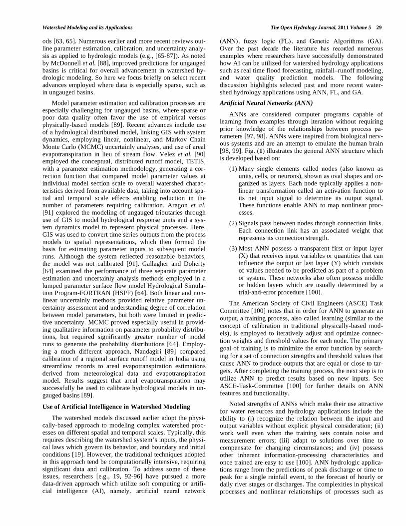
ANNs are considered computer programs capable of learning from examples through iteration without requiring prior knowledge of the relationships between process pa-rameters [97, 98]. ANNs were inspired from biological nerv-ous systems and are an attempt to emulate the human brain [98, 99]. Fig. (1) illustrates the general ANN structure which is developed based on:

(1) Many single elements called nodes (also known as units, cells, or neurons), shown as oval shapes and or-ganized as layers. Each node typically applies a non-linear transformation called an activation function to its net input signal to determine its output signal. These functions enable ANN to map nonlinear proc-esses.

(2) Signals pass between nodes through connection links. Each connection link has an associated weight that represents its connection strength.

(3) Most ANN possess a transparent first or input layer (X) that receives input variables or quantities that can influence the output or last layer (Y) which consists of values needed to be predicted as part of a problem or system. These networks also often possess middle or hidden layers which are usually determined by a trial-and-error procedure [100].

The American Society of Civil Engineers (ASCE) Task

Committee [100] notes that in order for ANN to generate an

output, a training process, also called learning (similar to the

concept of calibration in traditional physically-based mod-

els), is employed to iteratively adjust and optimize connec-

tion weights and threshold values for each node. The primary

goal of training is to minimize the error function by search-

ing for a set of connection strengths and threshold values that

cause ANN to produce outputs that are equal or close to tar-

gets. After completing the training process, the next step is to

utilize ANN to predict results based on new inputs. See

ASCE-Task-Committee [100] for further details on ANN features and functionality.

Noted strengths of ANNs which make their use attractive for water resources and hydrology applications include the ability to (i) recognize the relation between the input and output variables without explicit physical consideration; (ii) work well even when the training sets contain noise and measurement errors; (iii) adapt to solutions over time to compensate for changing circumstances; and (iv) possess other inherent information-processing characteristics and once trained are easy to use [100]. ANN hydrologic applica-tions range from the predictions of peak discharge or time to peak for a single rainfall event, to the forecast of hourly or daily river stages or discharges. The complexities in physical processes and nonlinear relationships of processes such as

30 The Open Hydrology Journal, 2011, Volume 5 Daniel et al.

rainfall-runoff and evapotransporation were found to lend themselves to ANN modeling [11, 101-103]. These ANN-based models have been considered an alternate to physically based models due to their simplicity relative to minimizing the need for collecting detailed watershed data [102]. The major advantage of ANN over conventional methods is the ability to model physical processes without the need for de-tailed information [104].

In the 1990s and early 2000s, several research efforts [e.g., 11, 103, 105-108] have shown ANN can be applied effectively across different aspects of water resources and hydrology. Hjelmfelt and Wang [105, 106] were among the first researchers to demonstrate the utility of ANNs in mod-eling these water resources processes. Here, they were able to use rainfall and runoff data from 24 large storm events chosen from the Goodwater Creek watershed (12.2 km

2) in

central Missouri to trainand test the ANNs. Results revealed that ANNs were able to generate a unit hydrograph better than those obtained through a standard gamma function rep-resentation. Smith and Eli [107] were able to incorporate the spatial and temporal distribution information of rainfall into a ANN model that predicted peak discharge and time to peak over a hypothetical watershed which was represented as a grid of cells. Using this method, they found the prediction of the entire hydrograph to be very accurate for multiple storm events. Riad et al. [109] showed that ANN-based models were better than classical regression models for simulating rainfall-runoff relations for a semiarid climate catchment area in Morocco. Recent work by Wang et al. [110] con-cluded that ANN models not only out performed other evapotransporation approximations developed in the semi-arid region of Burikan Faso, but they can also be utilized in developing countries with adverse climatic conditions [110]. Other studies [104, 111, 112] found that ANN models can predict evapotranspiration and perform better than the Pen-man-Monteith technique and other conventional methods.

Despite the demonstrated benefits of ANN, there are two key challenges that should be mentioned. First, ANN are usually implemented with a trial and error approach which tend to be extremely time consuming [113]. May and Siva-kumar [114, 115] highlighted this issue while investigating the application of ANN and multi-linear regression models

for predicting urban stormwater quality at unmonitored catchments. They concluded that both models generated similar prediction results but the regression model appeared to represent a more applicable approach since it was (i) faster to construct and apply; (ii) more transparent; and (iii) less likely to fit the limited data. The second limitation of ANNs identified by Moghaddamnia et al. [112] referenced the complicated input selection process. They gained some suc-cess by using a gamma test to address this problem, explor-ing different combinations of input data to assess their influ-ence on evaporation estimation modeling, showing that the gamma test greatly reduced model development require-ments, enabling provision of input data guidance prior to model development. Despite these promising results, they suggest that further evaluation is needed, especially with respect to its ability to assess validated data.

Genetic Algorithms (GA)

Genetic Algorithms (GA) are nonlinear optimization search techniques that imitate biological evolution processes of natural selection and survival of the fittest [116, 117]. The major difference between GAs and the other classical opti-mization techniques is that GAs work with a population of possible solution while classical optimization techniques work with a single solution [118]. Soman et al. [119] sum-marize the process of creating GAs in the following steps:

(1) Generate a random number of solution samples,

collectively called the population, within the feasi-

ble search space. Each of these samples, called a

chromosome, is defined by a sequence of decision

variables known as genes (can be in binary strings

of ones and zeros of user specifiedlength, or real

value numbers or integers).

(2) Each chromosome is assigned a measure of fit-

ness, based on the objective function value. These

chromosomesare referred to as species of the first

generation. For a maximization problem, the higher

the fitness values, the higher the chance for sur-

vival.

(3) Create the next generation of chromosomes.

This is accomplished by ranking the first genera-

tion chromosomes in ascending order of their fit-

Fig. (1). Configuration of feed forward three-layer ANN (adapted after: ASCE Task Committee [100]).

La

H

Layer

Outp

Layer

Network Network

Output

Input

Layer

Hidden

Layer

Output

Layer

Network

Input

X

Network

Output

Y

Watershed Modeling and its Applications The Open Hydrology Journal, 2011 Volume 5 31

ness value for a minimization problem, and in de-

scending order of their fitness for a maximization

problem. Chromosomes with the highest fitness

value will be given a higher probability to obtain a

mate, so as to produce offspring that may better fit

the environment. This process of selecting mates is

called selection. Once mates are selected, genes of

corresponding mates, or parents, are systematically

exchanged with the conception that the resulting

solutions or offsprings will have higher fitness val-

ues. The process of creating new individuals by

systematically assigning genes of chosen mates to

the new individuals is known as crossover. The

new chromosomes replace the old chromosomes,

which have low fitness values.

The process of selection and crossover is repeated for

many generations with the objective of reaching the global

optimal solution after a sufficient number of generations.

Other general forms of the GA include Genetic Program-

ming (GP) and Gene Expression Programming (GEP) which

are explained in more detail by Koza [120] and Ferreira [121].

Several early research efforts demonstrated the useful-

ness of GA in water resources applications. Ritzel et al.

[118] adopted GA to solve groundwater pollution problems.

Wang and Zheng [95] and Wu et al. [96] used GA-based

functions to solve a groundwater management model. Other

researchers [e.g., 122-128] made additional achievements in

developing or improving rainfall-runoff models using GA.

Wang [127] was successful in using GA with a local search

method to calibrate the Xinanjiang rainfall-runoff model.

Drecourt [126] investigated the GP approach for flow predic-

tion on the Kirkton catchment in Scotland (United Kingdom)

and found that the results compared favorably with two op-

timally calibrated conceptual models. Whigham and Crapper

[128] compared a GP-based rainfall-runoff model with a

deterministic lumped parameter model, based on the unit

hydrograph and found the results to be favorable as well.

Efforts by Liong et al. [124] were instrumental in demon-

strating GP as a new paradigm in rainfall-runoff modeling.

They showed GP-based rainfall runoff relationships can

serve as alternatives to conventional (physically based and

conceptual) rainfall runoff models. In Singapore, Muttil and

Liong [125] were able to apply GA programming to generate

empirically the underlying equations which connect input to output for the Upper Bukit Timah watershed.

More recent research efforts [e.g., 19, 129-132] continue

to demonstrate the utility of GA in support of water re-

sources applications. Guven et al. [131] developed a new

GP-based model for estimating reference evapotranspiration

in northern California by using five daily atmospheric vari-

ables (daily solar radiation, daily mean temperature, average

daily relative humidity and wind speed). They concluded that

the new model results were in good agreement with conven-

tional evapotranspiration models (here, the Penman-

Monteith equation, Hargreaves-Samani equation, solar radia-

tion-based ET equation, Jensen-Haise equation, Jones-

Ritchie equation, and Turc method) and can be used as an

alternative approach. It was also concluded that the GP-

based model offered a fast and practical method for accu-

rately estimating evapotransporation [131].

Yao and Yang [132] note that the complexity of parame-ter optimization for a distributed watershed model goes far beyond the capability of traditional optimization methods. To address this problem, a new GA-based optimization method was developed and tested using the Distributed-Hydrology-Soil-Vegetation model (DHSVM). Results of this effort demonstrate the feasibility of GA in optimizing pa-rameters of the DHSVM model. Hejaziet al. [129] and Preis and Ostfeld [19] demonstrated that GA can be coupled with other flow or water quality models to develop and augment calibration schemes.

Guven [130] investigated the use of linear genetic pro-gramming (a variant of GP) for predicting time-series of daily flow rates the Schuylkill River at Berne, PA, USA and found that the results showed good agreement with observed data. Results also showed that the GP-based model out per-formed an ANN-based model. These findings demonstrate GP’s promise for predicting the nonlinear and dynamic river flow parameters [130].

Although GAs have proven to be an effective and power-ful problem-solving strategy, they possess several limita-tions. The common thread in many of the difficulties with GAs has to do with their significant dependence on control parameters such as population size, crossover probability, and choice of crossover operator [133]. Jackson and Norgard [133] summarize these issues as follows:

(1) A GA may not know when it is done or lack proof of convergence. One possible way to deal with this problem is to examine a series of consecu-tive generations for solution improvement.

(2) GAs need to maintain a large population of solu-tions which provides the genetic diversity needed to adequately explore the solution space. Too small a population will result in premature convergence on a local minimum. While large populations enable superior performance, they also require more mem-ory and more execution time.

(3) Excessive reliance on crossover to introduce new genetic material can also result in premature convergence. The dominance of crossover as the principal stochastic process may cause the popula-tion to become more homogeneous, and thus stag-nating the evolutionary process.

(4) GAs are also known to have poor performance in climbing local hills in the solution space which results in reducing accuracy for many real-valued problems. This difficulty is a byproduct of the sole dependence of the algorithm on stochastic processes to improve solutions rather than on an analytical approach.

Jackson and Norgard [133] suggest that these limitations of GAs can be addressed effectively by combining GAs with other algorithms and techniques.

Fuzzy Logic (FL)

The FL approach to modeling is based on the theory of fuzzy sets [134], where relationships are defined verbally

32 The Open Hydrology Journal, 2011, Volume 5 Daniel et al.

instead of using known governing physical relationships. Classic set theory assigns an item as a member of a set (1) or a non-member of a set (0), while a fuzzy set allows for gra-dations between full membership and full non-membership. The main idea is to define the fuzzy membership functions which define relationships between input variables and out-puts of a system [135]. Mahabir et al. [135] identify the main steps for creating a FL-based modeling system as follows:

(1) A membership function must be defined for each variable (input and output). The membership function de-fines the degree to which the value of a variable belongs to the group and is usually a linguistic term, such as high, me-dium, or low.

(2) The membership functions are related by statements or rules, typically a series of IF–THEN statements. For ex-ample, one rule would be: IF the rainfall is low (linguistic term represented by a membership function) THEN the run-off (output) is low (linguistic term represented by a member-ship function).

(3) Each rule is evaluated through a process called impli-cation, and the results of all of the rules are combined in a process called aggregation.

(4) The resulting function is evaluated for a resulting value or score for the output variable (e.g., runoff) through a process called defuzzification.

The two main FL-based modeling systems included are:

(i) fuzzy inference systems, which work on already con-

structed rule-base mainly on the basis of expert knowledge,

and (ii) fuzzy adaptive systems, which can also build and

adjust rule-base automatically based on sample or training

data. Two significant advantages of FL–based models are their ability to be error tolerant and integrate expert knowl-

edge from water resource specialists [94]. Guertin et al.

[136] also point out that the FL approach is well suited to

watersheds studies as many environmental factors are best

expressed as gradients.

Like ANN and GA, the FL technique does have its limi-

tations. Three key disadvantages were identified in the litera-ture and presented here. Casper et al. [94] note that the larg-

est disadvantage of the fuzzy adaptive systems is its inability

to extrapolate without detailed expert knowledge about the

watershed system or process being simulated. The second

disadvantage of fuzzy inference and fuzzy adaptive (aug-

mented with expert knowledge) systems is their strong reli-

ance on subjective inputs from experts which might provide

more opportunity for their abuse [137]. Ferson and Tucker [138] also note that FL-based systems may also fail to cap-

ture the value range of complex data sets and the correlations

among parameters. Further details on FL theory and applica-

tions are provided in Zimmermann [139] and Dubois and

Prade [140].

According to Yu and Yang [76], FL can be applied to

hydrologic modeling where a hydrologist defines the accept-able degree of a simulation in the form of linguistic expres-

sions such as ‘bad’ and ‘good’ based on their knowledge or

expert judgment. Researchers have been successful in their

early attempts at applying FL for solving water resource

problems or modeling hydrologic processes including infil-

tration [141], contaminant fate and transport [142], recon-

struction of missing precipitation events [143] river level and

flood forecasting [144, 145], rainfall-runoff modeling [76,

146, 147], daily future water demand modeling [148],

drought classification [149], and regional drought prediction

[150].

More recent research trends in the utilization of the FL modeling approach highlight additional efforts targeted at combining other AI methods in hybrid systems. Chang et al. [151] developed a FL based method that was applied to pre-cipitation interpolation and utilized GA to determine parame-ters for the FL functions which represent locations without rainfall records and their surrounding rainfall gauges. Cheng et al. [80] combined FL-GA methods to develop a rainfall-run model while Chidthong et al. [152] and Chen et al. [93] utilized similar methods to forecast flooding. Combining FL and ANN also offer options for improving modeling tech-niques and managing water resource problems. For example, Tayfur and Singh [153] demonstrated that FL-ANN based models can be useful in simulating event based rainfall run-off on a watershed scale and are much easier to construct than the models based on the well-know kinematic wave approximation method. Chang and Chang [154] utilized an adaptive neuro-fuzzy (FL and ANN) inference system for predicting water levels in reservoirs. Firat and Gungor [155] also investigated the use of similar systems for estimating river flows. Chidthong et al. [152] were successful in devel-oping a hybrid system using FL, ANN, and GA for predict-ing peak flooding.

Spatial Considerations in Watershed Modeling

As previously mentioned, watershed modeling involves a

holistic approach that involves not only examining surface

hydrology, groundwater hydrology, or their interface as

whole systems, but attempting to imitate the three regions as

one system. Scale-up of each of these regions from the water

body (lake, river, stream, etc.) or aquifer to an entire catch-

ment or watershed presents obvious problems. One limita-

tion is the availability of precipitation, flow, land cover, etc.

data for the entire region. Another consideration is the lim-

ited understanding of the interactions between smaller hydro-

logic entities. Several studies have examined the effects of

scaling in watershed modeling [156-161]. Furthermore, the

scale or resolution of data used can impact the accuracy of

the model results [161-163]. The following sections high-

light the more prominent issues relating to scale and data

resolution in watershed modeling.

Scale-up from Hydrologic Models to Watershed Models

Much work has been done to conceptualize watershed in-teractions at the hillslope (sub-catchment) level resulting in

highly complex relationships from field experimentation.

Some suggest that watershed models should maintain this complexity and efforts should be made to ensure that the

smaller scale relationships are somehow incorporated into

the mesoscale watershed models [164]. Unfortunately, data limitations, computational complexity, and financial con-

straints limit the amount of information that may be gathered

from the field to represent entire watersheds. Bloschl and Sivapalan [158] published a review of scale issues in hydro-

logical modelling at the catchment level in 1995. In this,

discussions on simplification versus aggregation of hydro-

Watershed Modeling and its Applications The Open Hydrology Journal, 2011 Volume 5 33

logic parameters, scale up versus scale down, and the linkage

across various modelling scales are presented.

Problems associated with scale-up of hydrologic proc-esses to the watershed-scale include generalization and over parameterization. Through generalization or simplification, processes and variables that are applicable to a small portion of the watershed may be applied to the entire region. In this, the true representation of processes taking place may be lost. Over parameterization occurs when the watershed is repre-sented by multiple (possibly many) parameters/variables to the point that a holistic representation of the region is no longer present [158]. While Jakeman and Hornberger [165] suggest only a few parameters are identifiable/necessary for hydrologic models, van Werkhoven et al. [166] argue that the number of parameters necessary for watershed modeling is dependent on the focus of the model and experimental design. They suggest use of sensitivity analysis and thorough investigation on the model behaviour to determine the ap-propriate level of parameters involved to represent the water-shed.

Sivapalan [164] suggests that identification of common patterns, or features found at the hillslope scale within a watershed can be applied to larger regions to assist in scale-up to the watershed level. In addition, Wong [167] recommends use of physically-based models to replace empirical models noting that during scale-up from empirical hydrologic models to watershed-scale models physically-based relationships can be used to bridge the gaps. Kalin et al. [168] state that the spatial scale of the catchment is directly proportional to the complexity involved in modelling hydrologic processes of rainfall-runoff and surface erosion. Whether a lumped or semi-distributed model is used is dependent on the level of detail desired in the output and data available for representing the watershed.

Impacts of Data Resolution

Modeling the hydrologic responses over a watershed re-

quires use of soil maps and/or soil surveys to provide infor-

mation on the distribution of soil types and thus soil hydro-

logic properties. Previously, soil maps produced from sur-

veys of the region were the only source of this information.

Now, remote sensing (RS) and digital terrain analysis can be

utilized through geographic information system (GIS) tech-

niques [169] which are more accurate with higher resolution

data than previous methods. In addition, the availability of

precipitation data may be sparse and limiting. Gathering

measurements over a large area may not be economically

feasible, so modelers use genetic algorithms or other tech-

niques discussed previously to fill gaps and provide better representation of data over the entire watershed area.

Often, digital elevation models (DEMs) are used to iden-

tify stream networks/rivers and the land slopes that contrib-

ute flow to these waterbodies. DEMs can be publicly ob-

tained at various resolutions (e.g., 250 m, 500 m, 1000 m),

which can impact the accuracy of hydrograph generation and

identification of tributaries/river networks [163]. DEMs are

digital surfaces representing the area of interest with a grid

of given resolution placed over the surface and elevation data

assigned to each cell. Each DEM grid cell drains a specific

direction based upon its slope and the slope of the cells

around it. Streams or channel networks are identified by us-

ing the slope information of DEM grid cells and assigning a

threshold area (the minimum area that would drain to a point

for a stream channel to form). The stream network is com-

prised of a set of points that have summed areas of cells

above the threshold value draining toward them. The resolu-

tion of the DEM can impact the slope of grid cells due to the

area covered and averaging of elevations, and thus, the iden-

tification of stream networks [168, 170]. DEM resolution

also impacts the delineation of the watersheds. Ridge lines

are commonly used to define watersheds because these rep-

resent the divide for which portion of precipitation flows in which direction.

In a study by Zhu and Mackay [169], the impacts of us-ing traditional soil maps versus soil information derived from both fuzzy logic and digital elevation models (DEMs) were evaluated for the Lubrecht area in Montana. Using the newer technology, they found that peak runoff was reduced thus producing more realistic hydrographs. Yang et al. [163], evaluated the effects of DEM resolution on geomorphic properties (i.e., identification of river networks and hydro-logical response). In their study, fifteen catchments in Japan were analyzed using differing DEM resolutions. An increase in DEM mesh size (less resolution) led to loss in the amount of tributaries identified, flatter topography due to averaging of elevations for individual DEM grid cells and less accurate representation of the hydrological response of the catchment [163].

The required resolution of data used in the modeling ef-fort may be dependent on the output desired. Kalin et al. [168] evaluated the resolution required for different outputs for two U.S. Department of Agriculture (USDA) experimen-tal watersheds. When the peak runoff is the primary concern, the highest resolution is optimal. Meanwhile, if modelers are only interested in sediment load at the outlet, lower resolu-tion of model input data may be used.

Hydrologic and Hydrodynamic Models for Watershed Modeling

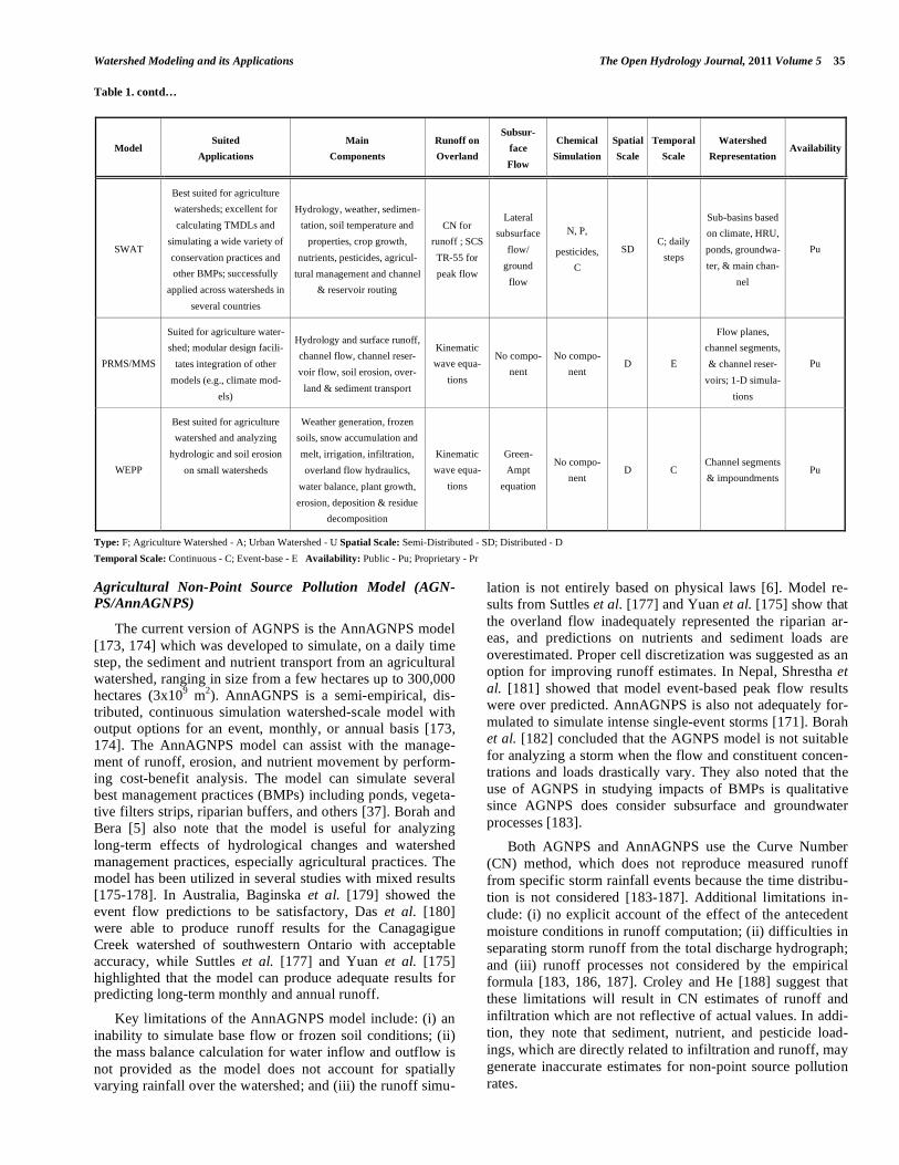
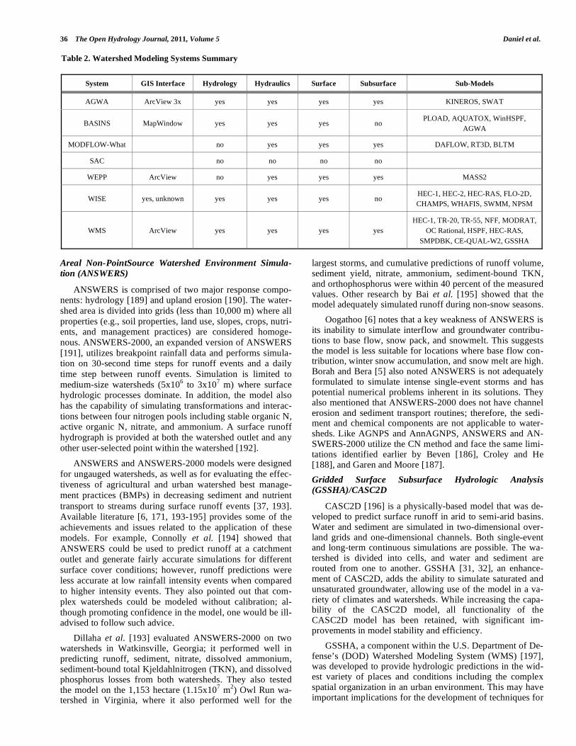
This section provides a review of current state-of-the-art of watershed-scale models, including discussion of their strengths and weaknesses when applied to various watershed and related problems. Recent reviews by Singh and Wool-hiser [39], Borah and Bera [171], Kalin and Hantush [37], Singh and Frevert [172], and Oogathoo [6] identify the more commonly used watershed-scale models: AGNPS (Agricul-tural Non-point Source)/AnnAGNPS (Annualized Agricul-tural Non-point Source), ANSWERS/ANSWERS-2000 (Area Non-point Source Watershed Environment Response Simulation), GSSHA (Gridded Surface Hydrologic Analy-sis)/CASC2D (CASCade of Planes in 2-Dimensions), HEC-1/HEC-HMS (Hydrologic Engineering Center’s Hydrologic Modeling System), HSPF (Hydrological Simulation Program – FORTRAN), KINEROS2 (KINematic Runoff and ERO-Sion), MIKE SHE (originally named SHE – Systéme Hy-drologique Européen), PRMS (Precipitation-Runoff Model-ing System), SWAT (Soil and Water Assessment Tool), and WEPP (Water Erosion Prediction Project). Each model’s attributes and example applications are discussed in detail in the following text, while Table 1 provides a summary of primary model characteristics and features.

34 The Open Hydrology Journal, 2011, Volume 5 Daniel et al.

Table 1. Watershed Models - Main Characteristics and Features

Model Suited

Applications

Main

Components

Runoff on

Overland

Subsur-

face

Flow

Chemical

Simulation

Spatial

Scale

Temporal

Scale

Watershed

Representation Availability

ANSWERS

Suited for agriculture water-

sheds ; designed for ungaged

watershed

Runoff, infiltration, subsur-

face drainage, soil erosion,

interception & overland

sediment transport

Manning &

continuity

Equations

No compo-

nent

No compo-

nent D E

Square grids;

1-D Simulations Pu

ANSWERS-

2000

Suited for medium size

agriculture watersheds ;

designed for ungaged water-

shed; useful in evaluating

the effectiveness of BMPs;

capable of simulating trans-

formation and interactions

between four nitrogen pools

Runoff; infiltration, wa-

ter/river routing, drainage,

river routing, chemi-

cal/nutrient transport

Manning

equation

Darcy’s

equation

N,P, sedi-

ment trans-

port

D C Grid/cells Pu

AGNPS Suited for agriculture water-

sheds

Runoff, infiltration &

soil erosion/sediment

transport

CN, TR-55

for peak flow

No compo-

nent

No compo-

nent D E

Homogeneous

land areas Pu

AnnAGNPS

Suited for agriculture water-

sheds; widely used for

evaluating a wide variety of

conservation practices and

other BMPs

Hydrology, sediment, nutri-

ents and pesticide transport,

DEM used to generate grid

and stream network

CN, TR-55

for peak flow

Darcy’s

equation

N, P, pesti-

cides, orga-

niccar-

bon&nutrien

ts

D

C- daily

or

sub-daily

steps

Homogeneous

land areas,

reaches, & im-

poundments

Pu

GSSHA/CAS

C2D

Suited for both agriculture

or urban watersheds; diverse

modeling capabilities in a

variety of climates and

watersheds with complex

spatial datasets

Spatially varying rainfall;

rainfall excess and 2-D flow

routing; soil moisture, chan-

nel routing, upland erosion, &

sediment transport

2-D diffusive

wave equa-

tions

No compo-

nent

No compo-

nent D E; C

2-D square over-

land grids; 1-D

channels

Pr

HEC-1/HEC-

HMS

Suited for urban watersheds;

widely used for modeling

floods and impacts on land

use changes

Precipitation, losses,

baseflow, runoff transforma-

tion & routing

CN, kine-

matic wave

equations

No compo-

nent

No compo-

nent SD E

Dendritic network

or grid Pu

HSPF

Suited for both agriculture

or urban watersheds; diverse

water quality and sediment

transport at any point on the

watershed

Runoff /water quality con-

stituents, simulation of pervi-

ous/impervious areas, stream

channels & mixed reservoirs

Empirical

outflow

Interflow

outflow,

percolation;

groundwater

outflow

Soil/water

temp., DO,

CO2, N,

NH3, or-

ganic N/P,

N/P, pesti-

cides

SD C.

Pervious

/impervious land

areas, stream

channels, &

mixed reservoirs;

1-D simulations

Pu

KINEROS2

Suited for urban environ-

ments and studying impacts

of single sever or design

storm even; Also can be

applied to agriculture water-

sheds.

Distributed rainfall inputs,

rainfall excess, overland flow,

channel routing, sediment

transport, interception, infil-

tration, surface runoff &

erosion

Kinematic

wave equa-

tions

No compo-

nent

No compo-

nent D E

Cascade of planes

& channels; 1-D

simulations

Pu

MIKE SHE

Wide range of spatial and

temporal scales; modular

design facilitates integration

of other models; advanced

capabilities for water qual-

ity, parameter estimation

and water budget analysis

Interception, over-

land/channel flow, unsatu-

rated/saturated zone, snow-

melt; aquifer/ rivers ex-

change, advection/dispersion

of solutes, geochemical

processes, plant growth, soil

erosion & irrigation

2-D diffusive

wave equa-

tions

3-D

groundwa-

ter flow

Dissolved

conservative

solutes

in surface,

soil, &

ground

waters

D

E; C;

variable

steps

2-D rectangular

/square overland

grids; 1-D chan-

nels;

1-D unsaturated/

3-D saturated

flow

Pr

Watershed Modeling and its Applications The Open Hydrology Journal, 2011 Volume 5 35

Table 1. contd…

Model Suited

Applications

Main

Components

Runoff on

Overland

Subsur-

face

Flow

Chemical

Simulation

Spatial

Scale

Temporal

Scale

Watershed

Representation Availability

SWAT

Best suited for agriculture

watersheds; excellent for

calculating TMDLs and

simulating a wide variety of

conservation practices and

other BMPs; successfully

applied across watersheds in

several countries

Hydrology, weather, sedimen-

tation, soil temperature and

properties, crop growth,

nutrients, pesticides, agricul-

tural management and channel

& reservoir routing

CN for

runoff ; SCS

TR-55 for

peak flow

Lateral

subsurface

flow/

ground

flow

N, P,

pesticides,

C

SD C; daily

steps

Sub-basins based

on climate, HRU,

ponds, groundwa-

ter, & main chan-

nel

Pu

PRMS/MMS

Suited for agriculture water-

shed; modular design facili-

tates integration of other

models (e.g., climate mod-

els)

Hydrology and surface runoff,

channel flow, channel reser-

voir flow, soil erosion, over-

land & sediment transport

Kinematic

wave equa-

tions

No compo-

nent

No compo-

nent D E

Flow planes,

channel segments,

& channel reser-

voirs; 1-D simula-

tions

Pu

WEPP

Best suited for agriculture

watershed and analyzing

hydrologic and soil erosion

on small watersheds

Weather generation, frozen

soils, snow accumulation and

melt, irrigation, infiltration,

overland flow hydraulics,

water balance, plant growth,

erosion, deposition & residue

decomposition

Kinematic

wave equa-

tions

Green-

Ampt

equation

No compo-

nent D C

Channel segments

& impoundments Pu

Type: F; Agriculture Watershed - A; Urban Watershed - U Spatial Scale: Semi-Distributed - SD; Distributed - D

Temporal Scale: Continuous - C; Event-base - E Availability: Public - Pu; Proprietary - Pr

Agricultural Non-Point Source Pollution Model (AGN-

PS/AnnAGNPS)

The current version of AGNPS is the AnnAGNPS model

[173, 174] which was developed to simulate, on a daily time

step, the sediment and nutrient transport from an agricultural

watershed, ranging in size from a few hectares up to 300,000

hectares (3x109 m

2). AnnAGNPS is a semi-empirical, dis-

tributed, continuous simulation watershed-scale model with

output options for an event, monthly, or annual basis [173,

174]. The AnnAGNPS model can assist with the manage-

ment of runoff, erosion, and nutrient movement by perform-

ing cost-benefit analysis. The model can simulate several

best management practices (BMPs) including ponds, vegeta-

tive filters strips, riparian buffers, and others [37]. Borah and

Bera [5] also note that the model is useful for analyzing

long-term effects of hydrological changes and watershed

management practices, especially agricultural practices. The

model has been utilized in several studies with mixed results

[175-178]. In Australia, Baginska et al. [179] showed the

event flow predictions to be satisfactory, Das et al. [180]

were able to produce runoff results for the Canagagigue

Creek watershed of southwestern Ontario with acceptable

accuracy, while Suttles et al. [177] and Yuan et al. [175]

highlighted that the model can produce adequate results for predicting long-term monthly and annual runoff.

Key limitations of the AnnAGNPS model include: (i) an

inability to simulate base flow or frozen soil conditions; (ii)

the mass balance calculation for water inflow and outflow is

not provided as the model does not account for spatially

varying rainfall over the watershed; and (iii) the runoff simu-

lation is not entirely based on physical laws [6]. Model re-

sults from Suttles et al. [177] and Yuan et al. [175] show that

the overland flow inadequately represented the riparian ar-

eas, and predictions on nutrients and sediment loads are

overestimated. Proper cell discretization was suggested as an

option for improving runoff estimates. In Nepal, Shrestha et

al. [181] showed that model event-based peak flow results

were over predicted. AnnAGNPS is also not adequately for-

mulated to simulate intense single-event storms [171]. Borah

et al. [182] concluded that the AGNPS model is not suitable

for analyzing a storm when the flow and constituent concen-

trations and loads drastically vary. They also noted that the

use of AGNPS in studying impacts of BMPs is qualitative

since AGNPS does consider subsurface and groundwater

processes [183].

Both AGNPS and AnnAGNPS use the Curve Number

(CN) method, which does not reproduce measured runoff

from specific storm rainfall events because the time distribu-

tion is not considered [183-187]. Additional limitations in-

clude: (i) no explicit account of the effect of the antecedent

moisture conditions in runoff computation; (ii) difficulties in

separating storm runoff from the total discharge hydrograph;

and (iii) runoff processes not considered by the empirical

formula [183, 186, 187]. Croley and He [188] suggest that

these limitations will result in CN estimates of runoff and

infiltration which are not reflective of actual values. In addi-

tion, they note that sediment, nutrient, and pesticide load-

ings, which are directly related to infiltration and runoff, may

generate inaccurate estimates for non-point source pollution

rates.

36 The Open Hydrology Journal, 2011, Volume 5 Daniel et al.

Areal Non-PointSource Watershed Environment Simula-

tion (ANSWERS)

ANSWERS is comprised of two major response compo-nents: hydrology [189] and upland erosion [190]. The water-

shed area is divided into grids (less than 10,000 m) where all

properties (e.g., soil properties, land use, slopes, crops, nutri-ents, and management practices) are considered homoge-

nous. ANSWERS-2000, an expanded version of ANSWERS

[191], utilizes breakpoint rainfall data and performs simula-tion on 30-second time steps for runoff events and a daily

time step between runoff events. Simulation is limited to

medium-size watersheds (5x106 to 3x10

7 m) where surface

hydrologic processes dominate. In addition, the model also

has the capability of simulating transformations and interac-

tions between four nitrogen pools including stable organic N, active organic N, nitrate, and ammonium. A surface runoff

hydrograph is provided at both the watershed outlet and any

other user-selected point within the watershed [192].

ANSWERS and ANSWERS-2000 models were designed

for ungauged watersheds, as well as for evaluating the effec-

tiveness of agricultural and urban watershed best manage-

ment practices (BMPs) in decreasing sediment and nutrient

transport to streams during surface runoff events [37, 193].

Available literature [6, 171, 193-195] provides some of the

achievements and issues related to the application of these

models. For example, Connolly et al. [194] showed that

ANSWERS could be used to predict runoff at a catchment

outlet and generate fairly accurate simulations for different

surface cover conditions; however, runoff predictions were

less accurate at low rainfall intensity events when compared

to higher intensity events. They also pointed out that com-

plex watersheds could be modeled without calibration; al-

though promoting confidence in the model, one would be ill-advised to follow such advice.

Dillaha et al. [193] evaluated ANSWERS-2000 on two watersheds in Watkinsville, Georgia; it performed well in predicting runoff, sediment, nitrate, dissolved ammonium, sediment-bound total Kjeldahlnitrogen (TKN), and dissolved phosphorus losses from both watersheds. They also tested the model on the 1,153 hectare (1.15x10

7 m

2) Owl Run wa-

tershed in Virginia, where it also performed well for the

largest storms, and cumulative predictions of runoff volume, sediment yield, nitrate, ammonium, sediment-bound TKN, and orthophosphorus were within 40 percent of the measured values. Other research by Bai et al. [195] showed that the model adequately simulated runoff during non-snow seasons.

Oogathoo [6] notes that a key weakness of ANSWERS is its inability to simulate interflow and groundwater contribu-tions to base flow, snow pack, and snowmelt. This suggests the model is less suitable for locations where base flow con-tribution, winter snow accumulation, and snow melt are high. Borah and Bera [5] also noted ANSWERS is not adequately formulated to simulate intense single-event storms and has potential numerical problems inherent in its solutions. They also mentioned that ANSWERS-2000 does not have channel erosion and sediment transport routines; therefore, the sedi-ment and chemical components are not applicable to water-sheds. Like AGNPS and AnnAGNPS, ANSWERS and AN-SWERS-2000 utilize the CN method and face the same limi-tations identified earlier by Beven [186], Croley and He [188], and Garen and Moore [187].

Gridded Surface Subsurface Hydrologic Analysis

(GSSHA)/CASC2D

CASC2D [196] is a physically-based model that was de-veloped to predict surface runoff in arid to semi-arid basins. Water and sediment are simulated in two-dimensional over-land grids and one-dimensional channels. Both single-event and long-term continuous simulations are possible. The wa-tershed is divided into cells, and water and sediment are routed from one to another. GSSHA [31, 32], an enhance-ment of CASC2D, adds the ability to simulate saturated and unsaturated groundwater, allowing use of the model in a va-riety of climates and watersheds. While increasing the capa-bility of the CASC2D model, all functionality of the CASC2D model has been retained, with significant im-provements in model stability and efficiency.

GSSHA, a component within the U.S. Department of De-fense’s (DOD) Watershed Modeling System (WMS) [197], was developed to provide hydrologic predictions in the wid-est variety of places and conditions including the complex spatial organization in an urban environment. This may have important implications for the development of techniques for

Table 2. Watershed Modeling Systems Summary

System GIS Interface Hydrology Hydraulics Surface Subsurface Sub-Models

AGWA ArcView 3x yes yes yes yes KINEROS, SWAT

BASINS MapWindow yes yes yes no PLOAD, AQUATOX, WinHSPF,

AGWA

MODFLOW-What no yes yes yes DAFLOW, RT3D, BLTM

SAC no no no no

WEPP ArcView no yes yes yes MASS2

WISE yes, unknown yes yes yes no HEC-1, HEC-2, HEC-RAS, FLO-2D,

CHAMPS, WHAFIS, SWMM, NPSM

WMS ArcView yes yes yes yes

HEC-1, TR-20, TR-55, NFF, MODRAT,

OC Rational, HSPF, HEC-RAS,

SMPDBK, CE-QUAL-W2, GSSHA

Watershed Modeling and its Applications The Open Hydrology Journal, 2011 Volume 5 37

runoff modeling, flood prediction, and planning in urbanized areas [31]. GSSHA has new or improved CASC2D features such as the ability to simulate major hydrologic storage units (e.g., lakes, wetlands, and reservoirs) and an improvement in the predictions of in-stream sediment transport, especially during large rainfall events [31]. Both models were tested on the Goodwin Creek Experimental Watershed in Mississippi where it was shown that the accuracy of sediment discharge for selected storms was superior when using GSSHA [31, 198]. Despite these results, other studies [e.g., 37] indicate that the model may have major limitations such as the poten-tial to generate very poor sediment results. Kalin and Han-tush [37] suggest erosion in channels is not transport limited, which means the model generates sediment that has a vol-ume greater than what the flow can carry. Another limitation for the model is its numerical schemes, which are computa-tionally intensive and demand large amounts of data [171]. According to Ogden and Julien [199], simulation times can become prohibitive when the number of model grid cells exceeds 100,000; therefore, the model may become prohibi-tive for medium to large-sized watersheds [171].

HEC-1/HEC-HMS

HEC-1, developed to simulate hydrologic processes (pre-cipitation, losses, baseflow, runoff transformation, and rout-ing) on watersheds ranging in size from 1 km

2 to 100,000

km2, produces runoff hydrographs at single or multiple loca-

tions on complex watershed networks for gauged and hypo-thetical rainfall events [200]. HEC-HMS (Hydrologic Engi-neering Center's Hydrologic Modeling System) [201, 202] is the “next generation" and state-of-the-art Windows-based model for precipitation-runoff simulation that will supersede the HEC-1 model. HEC-HMS provides a variety of options for simulating precipitation-runoff and routing processes, and is comprised of a Graphical User Interface (GUI) [203], integrated hydrologic analysis components, data storage and management capabilities, and graphics and reporting facili-ties [201, 202]. Both HEC-1 [200] and HEC-HMS [201] have been widely used for modeling floods and impacts on land use changes [6]. Duru and Hjelmfelt [204], using the model's kinematic wave method, found that even with lim-ited calibration, runoff prediction for ungauged catchments was good and impacts of land use on the hydrologic cycle could be evaluated accurately. Additionally, a study con-ducted in northern Ontario, Canada showed that HEC-1 model could be used for runoff simulation in an ungauged watershed [205].

Even though HEC-1/HEC-HMS has been widely used, Oogathoo [6] notes that it excludes certain important fea-tures. The model is constrained to a constant time step, which may not be suitable for components requiring detailed analysis. Since it is semi-distributed, the model assumes hy-drologic processes to occur uniformly within each sub-basin. Also, as the primary purpose of the model is to determine flood hydrographs, a simple method is used for the baseflow simulation; therefore, the loss component of the model is not tracked down in absence of precipitation, that is, the soil does not dry out and recover its loss potential. Other limita-tions identified by Scharffenberg [201] include uncoupled models for evapotranspiration-infiltration and infiltration-base flow processes, no aquifer interactions, the allowance, but limited capability, of flow splits within the dendritic

stream systems, and the lack of downstream flow influence or reversal which makes backwater possible but only if con-tained within a reach.

Hydrological Simulation Program-Fortran (HSPF)

HSPF [206, 207] is a semi-distributed, continuous model that simulates hydrologic and associated water quality proc-esses on pervious and impervious land surfaces, in streams, and in well-mixed impoundments where water movement is simulated as overland flow, interflow, and groundwater flow. Also simulated are snowpack depth and water content, snowmelt, evapotranspiration, ground-water recharge, dis-solved oxygen, biochemical oxygen demand, temperature, pesticides, conservatives, fecal coliforms, sediment detach-ment and transport, sediment routing by particle, size, chan-nel routing, reservoir routing, constituent routing, pH, am-monia, nitrate-nitrite, organic nitrogen, orthophosphate, or-ganic phosphorous, phytoplankton, and zooplankton. The model utilizes hydrological response units (HRUs) based on uniform climate and storage capacity factors. Periods from a few minutes to hundreds of years can be simulated. Simulation results include a time history of the runoff flow rate, sediment load, and nutrient and pesticide concentrations, along with a time history of water quantity and quality at any point in a watershed. HSPF simulates three sediment types (sand, silt, and clay) in addition to a single organic chemical and transformation products of that chemical [206, 207].

Generally used to assess the effects of land use change, reservoir operations, point or non-point source treatment alternatives, and flow diversions [37], HSPF is also suitable for mixed agricultural and urban watersheds [171]. Some of the key strengths of the model identified by Aqua Terra [208] include: (i) a comprehensive representation of water-shed land, stream processes, and watershed pollutant sources, including non-point (by multiple land uses), point, and atmospheric sources; (ii) flexibility and adaptability to a wide range of watershed conditions; and (iii) well-designed code modularity and structure. Oogathoo [6] and AquaTerra [208] note that HSPF’s key limitations derive from it not being fully distributed or physically-based. As a result, wa-tershed characteristics and climatic parameters are lumped into several units, and both empirical and physical equations are used to simulate the water flow [6]. In addition, due to its conceptualization of the overland (sub-basin) areas as lev-eled detention storage and use of the storage-based or non-linear flow equations in routings, HSPF is not adequate for simulating intense single-event storms, especially for large sub-basins and long channels [6, 171]. The model requires extensive data requirements (e.g., hourly rainfall) and avail-able documentation provides no comprehensive parameter estimation guidance. As a result, user training is normally required [208]. In their effort to evaluate the model, Saleh and Du [209] highlighted these issues as they found the cali-bration process tends to be strenuous and long.

Kinematic Runoff and Erosion Model (KINEROS2)

Represented by a cascade of planes and channels, KINEROS2 may be used to determine the effects of various artificial features such as urban developments, small deten-tion reservoirs, or lined channels on flood hydrographs and sediment yield [33]. The model is also adopted as part of the

38 The Open Hydrology Journal, 2011, Volume 5 Daniel et al.

Automated Geospatial Watershed Assessment Tool (AGWA) software system [210, 211]. Limited to Hortonian flow and not designed for long-term simulations, KINEROS2 lacks an evapotranspiration component impor-tant for the mass balance of the water cycle [37]; however, with its complete set of hydrology and sediment components, the model serves as a useful tool for studying single severe or design storms and evaluating watershed management practices, especially structural practices [171]. Using a small U.S. Department of Agriculture (USDA) experimental wa-tershed located near Treynor, Iowa, Kalin and Hantush[37] tested the model and showed that it was also extremely ro-bust in simulating erosion and sediment transport. The model was designed for arid and semi-arid areas [212]; however, several studies [210, 213-215] highlight the ability of the model to successfully simulate erosion, sediment transport, and characterize the runoff response of the watershed due to changes of land cover in arid and semi-arid watersheds. La-jili-Ghezal [215] conducted similar assessments on the M'Richet El Anze watershed in a Tunisian semi-arid area and concluded that the model was adequate for predicting runoff from ungauged watersheds and for evaluating future land use master-plans for Tunisian semi-arid high lands. Miller et al. [210] also used KINEROS2 within the AGWA framework to successfully assess increased event runoff vol-umes and flashier flood response in watersheds that contrib-ute runoff to the upper San Pedro River in Sonora, Mexico and southeast Arizona.

Unlike most of the studies mentioned, Al-Qurashiet al.

[212] were less successful when assessing the model using

data from a large arid catchment in Oman. Despite relatively

extensive and high resolution rainfall-runoff data, and their

efforts to optimize performance using automatic calibration

and by adding a rainfall parameter, the model validation per-

formance was poor, and in general, no better than achieved

using a ‘default’ parameter set [212]. Borah and Bera [5]

note that the model does a relatively good job of simulating

runoff and sediment yield at watershed scales of up to ap-

proximately 1,000 hectares (1x107 m

2); however, such poor

results may arise since applications of the model are limited

to small watersheds and specific combinations of space and

time increments for maintaining stability of the numerical

solutions. Overall, a key weakness of the model is the ab-

sence of chemical/nutrient components [171] which limit its capabilities to simulate for BMPs [37].

MIKE SHE

MIKE SHE is a fully integrated, distributed, and physi-cally-based watershed model that simulates the major proc-esses in the hydrologic cycle and includes process models for evapotranspiration, overland flow, unsaturated flow, ground flow, channel flow, and their interactions [34]. It is used mostly at the watershed scale and from a single soil profile to several sub-watersheds with different soil types [216, 217]. The model's distributed nature allows a spatial distribution of watershed parameters, climate variables, and hydrological response through an orthogonal grid network and column of horizontal layers at each grid square in the horizontal and vertical, respectively [218]. The model can be used for storm or long-term events with a variable time step. Being physi-cally-based, the topography, along with watershed character-istics such as vegetation and soil properties, is included in

the model. With a modular structure, MIKE SHE is capable of exchanging data between components as well as adding new process model components. The flexible operating structure of MIKE SHE allows the use of as many or as few components of the model, based on availability of data [219].

MIKE SHE is considered the most comprehensive water-shed model with virtually all of the in-surface and surface phases of the hydrologic cycle [37]. It also has many of the options to simulate wetlands, and nutrient and pesticide management. The model is being used for a wide variety of applications in different countries, including England [220], Australia [221], Canada [6], and the United States [222]. Some of the notable application areas include river basin management and modeling [223], integrated ground/surface water modeling [221, 222], irrigation [224-226], land use changes, and anthropogenic effects [27].

Thompson et al. [220] used the model simulated in a wet-land in England and found that the simulation results consis-tently matched the observed data and reproduced the sea-sonal dynamics of groundwater and ditch water levels. Sahoo et al. [84] used the model in a mountainous region of Hawaii to study watershed response to storm events and found the results were comparable to the observed data. In addition, Demetriou and Punthakey [221] concluded that the model was accurate in predicting water movement from aquifers, drainage and supply systems, and land surfaces across an Australian watershed with a complex hydro-geological re-gime. Overall, Singh et al. [227] showed that the model can be utilized for irrigation planning and management of water resources for agricultural purposes.

Many of the MIKE SHE applications also involve cou-pling with other models; the model can interface with Model of Urban Sewers (MOUSE) to simulate the effect of urban drainage and sewer systems on the surface/subsurface hy-drology [34, 228, 229] and is also frequently coupled with (DAISY), a detailed soil-plant-atmosphere model for agricul-ture related studies [34, 230, 231]. Like the GSSHA model, MIKE SHE faces the problem of being computationally in-tensive and may be prohibitive for medium to large-sized watersheds [171]. Borah and Bera [5] further point out that the physically based flow-governing equations use approxi-mate numerical solutions, which are subject to computational instability problems, and limited on space and time incre-ments and watershed sizes.

Precipitation-Runoff Modeling System (PRMS)/Modular Modeling System (MMS)

PRMS [232] is a modular-design, deterministic, distrib-uted model that simulates precipitation- and snowmelt-driven movement of water through the watershed via over-land flow, interflow, and baseflow. Watershed response can be simulated at a daily time step or more frequently over the course of a storm. The watershed is divided into sub-units based on basin characteristics such as slope, aspect, eleva-tion, vegetation type, soil type, land use, and precipitation distribution. Two levels of partitioning are available for PRMS. The first divides the basin into HRUs based on the basin characteristics where water and energy balances are computed daily for each HRU; the sum of the responses of all HRU's, weighted on a unit-area basis, produces the daily system response and streamflow for a basin. A second level

Watershed Modeling and its Applications The Open Hydrology Journal, 2011 Volume 5 39

of partitioning is available for storm hydrograph simulation where the watershed is conceptualized as a series of inter-connected flow planes and channel segments. Surface runoff is routed over the flow planes into the channel segments and channel flow is routed through the watershed channel sys-tem. A HRU can be considered the equivalent of a flow plane or it can be delineated into a number of flow planes [232, 233]. PRMS was redesigned and now forms the basis of the US Geological Society (USGS) Modular Modeling System (MMS) [232].

PRMS [233] has been applied in different regions around the world. Applications range from the investigation of se-lected process components to streamflow simulation and the integration of MMS with other models [234]. One of the major benefits of MMS is its support for the integration of models and tools at a variety of levels [232]. Design levels include individual process models, tightly coupled models, loosely coupled models, and fully integrated decision sup-port systems [234]. Several studies [235-237] have focused on this aspect of the model with some success. Steuer and Hunt [236] and Hunt and Steuer [235] used the model to study the effects of urbanization and land use changes on ground water recharge, and explicitly fed the results into the U.S. Geologic Survey groundwater model, Modular Three-Dimensional Finite-Difference Ground-Water Flow Model(MODFLOW), for other studies in Dane County, Wis-consin. Hobson [237] coupled the model with a stochastic weather generator as a framework to simulate weather vari-ables and streamflows in the Upper Truckee River Basin on the California and Nevada border. The model can also be effectively used to evaluate the effects of climate variability, change on water resources, water management [234], and simulate floods including the representing flood wave propa-gation from single rainfall events [5]. Valeo and Xiang [238] demonstrated this capability by analyzing climate change impacts on flooding from the Elbow River watershed in the foothills of the Rocky Mountains. In addition, Yates et al. [239] utilized the model with historical radar rainfall and forecast data to simulate flash flooding on a watershed that was partially burned during a forest fire. Other examples of these studies were conducted in several regions of the world, including the Main Ethiopian Rift Valley [240], river basins in the Sierra Nevada of California [241], and the Arno River in Italy [242].

Borah and Bera [5] identified the following key weak-nesses of PRMS/MMS: (i) like KINEROS2, the model was designed for single rainfall events using one-dimensional flow equations and has potential numerical problems inher-ent to the numerical solutions; (ii) in the Storm Mode, the model has hydrology and overland sediment, but no chemi-cal component, sediment simulation in stream channels, and subsurface flow simulations; and (iii) the physically based flow-governing equations use approximate numerical solu-tions which are subject to computational instability prob-lems, and limited on space and time increments and water-shed sizes.

Soil and Water Assessment Tool (SWAT)

SWAT [35, 36] is a physically-based, continuous-time watershed model that operates on a daily time step and is designed to predict the impact of management on water, sediment, and agricultural chemical yields in ungauged wa-

tersheds. The watershed is divided into multiple subwater-sheds, which are then further subdivided into HRUs that consist of homogeneous land use, management, and soil characteristics. The HRUs represent percentages of the sub-watershed area and are not identified spatially within a SWAT simulation. Alternatively, a watershed can only be subdivided into subwatersheds that are characterized by dominant land use, soil type, and management. Output for the model includes evapotranspiration, soil water storage, and water yield (surface runoff plus subsurface flow) [35, 36]. The model has been adopted as part of the USEPA’s Better Assessment Science Integrating Point and Nonpoint Sources (BASINS) system [243] and AGWA [210, 211] software systems because it is a widely accepted continuous model suitable for agricultural and forest land uses [5, 168]. Based on these core strengths, Gassman et al. [36] found that the primary applications of SWAT are calibration and/or sensitivity analysis, climate change impacts, GIS interface descriptions, hydrologic assessments, variation in configura-tion or data input effects, comparisons with other models or techniques, interfaces with other models, and pollutant as-sessments. The foundation strength of SWAT in many of these applications is the combination of simplified upland and channel processes that are incorporated into the model noted by Gassman et al. [36]. The incorporation of the CN method and non-spatial HRUs supports model adaptation to virtually any watershed with a wide variety of hydrologic conditions [36].

SWAT has produced favorable model results when

evaluated on watersheds with a range of conditions in the

U.S. and many other countries such as Korea [244], Canada

[245], China [246], Finland [247], India [248-250], Tunisia

[251], and Greece [252]; across many of these watersheds,

SWAT has shown flexibility in simulating surface runoff.

For example, Du et al. [253] demonstrated that a modified

version of the SWAT model was able to generate reasonable

simulation results for surface and subsurface flows, water

table dynamics, tile flow, potholes, surface tile inlets, and

aeration stress on plants for large flat landscapes. Gebremes-

kel et al. [245] stated that the SWAT model performed very

well for stream flow prediction in the Canagagigue Creek

watershed of southwestern Ontario, Canada. Several studies

have also demonstrated the utility of SWAT as a tool for

evaluating how stream flow can be affected by climate change [254-256].

With a flexible framework, SWAT facilitates the calcula-tion of TMDLs and simulation of a wide variety of conserva-

tion practices and other BMPs (e.g., fertilizer and manure

application rate and timing, irrigation management, and flood prevention structures) [36]. Several studies illustrate

the success of SWAT in conducting these types of simula-

tions as part of an overall BMP assessment. For example, Santhi et al. [257] were able to use SWAT to determine the

impacts of manure and nutrient related BMPs, forage harvest

management, and other BMPs on water quality in the West Fork watershed in Texas. Chaplot et al.’s [258] efforts with

SWAT showed that the adoption of no tillage, changes in

nitrogen application rates, and land use changes had the po-tential to significantly affect nitrogen losses on the Walnut

Creek watershed in Iowa, and Kang et al. [244] were suc-

cessful in predicting and evaluating TMDLs of total nitro-

40 The Open Hydrology Journal, 2011, Volume 5 Daniel et al.

gen, total phosphorus, and suspended solid for a small water-

shed containing rice paddies.

SWAT possesses components that make it a robust tool for simulating in-stream water quality dynamics, bacteria fate and transport, and sediment transport [36]. A study con-ducted by Migliaccio et al. [259] compared SWAT’s in-stream water quality component with QUAL2E, USEPA’s well-known and state-of-the-art in-stream water quality model. Both options were used to simulate the movement of total phosphorous (P) and nitrate/nitrite (N) movement on War Eagle Creek watershed in Arkansas. The study revealed that there was no statistical difference between both in-stream water quality modeling options. Saleh and Du [209] and Stewart et al. [260] also show that SWAT predicted rea-sonable results for P and N loss on the Bosque River water-shed in Texas. Chu et al. [261] evaluated SWAT on the Warner Creek watershed in Maryland and generated simula-tion results for sediment loads which agreed strongly with yearly measured values. Other studies [248, 250, 262-265] on SWAT simulation of sediment loading on different water-sheds also generated comparable results. In Missouri, for example, Benham et al. [266] used SWAT to determine the bacteria sources and assess which BMPs can reduce the bac-teria on a watershed in Missouri. Similar results [267, 268] from other studies also highlight the usefulness of SWAT in bacteria fate and transport.

The examples presented here have highlighted the flexi-bility and robustness of SWAT. Despite these strengths, SWAT possesses a number of weaknesses, notably the use of non-spatial aspects of HRUs [6, 36]. As a result, Gassman et al. [36] note that this does not allow SWAT to provide an explicit spatial representation of riparian buffer zones, wet-lands, and other BMPs. In addition, there is limited ability to account for targeted placement of grassland or other land use and ignore flow and pollutant routing within a given subwa-tershed. Like ANPS and AnnANPS, SWAT also utilizes the curve number (CN) method and faces the same limitations identified earlier by Beven [186-188]. Borah and Bera [171] also report that SWAT does not simulate single-event storms adequately.

Water Erosion Prediction Project (WEPP)

WEPP [269] is a process-based, distributed, continuous,

erosion prediction model. It is applicable to hillslope erosion

processes (sheet and rill erosion), as well as simulation of the

hydrologic and erosion processes on small watersheds. The

primary intention of the model is to evaluate the effects of

farming and land use on soil erosion and sediment delivery

for small, agricultural field-sized watersheds (up to 2.59x106

m2). WEPP has been used in a wide range of applications,

including runoff mapping [270], sediment analysis [271],

and modeling the transport of pathogenic microorganisms

[272]. Another example of the WEPP application was fo-

cused on the connection between soil sediment and microbial

transport [272]. It was determined that areas with clay soils

contribute more to contamination of water supplies by mi-

croorganisms than those with sandy soils. It was also sug-

gested that the leading factors are hydraulic conductivity,

rainfall intensity, and topographic slope. Similar efforts

could be performed on organic chemicals that may adhere to differing soil types and be transported through the watershed.

A computer interface (Erosion Database Interface, EDI) was created by van Lier et al. [273] to process the surface hydrology output from WEPP into a georeferenced estima-tion of runoff. This tool allowed for improved management of agriculture and can be used to assess crop management techniques [270]. WEPP was used, along with the Universal Soil Loss Equation, sediment rating curves, and other model-ing techniques to develop a sediment budget for the Murder-CreekBasin in Georgia. From the study, researchers found that unstable streambanks, mobile streambeds, and turbidity currently observed in the area were the result of poor farm-ing practices from the early 1900s [271].

WATERSHED MODELING SYSTEMS

There are numerous watershed-scale hydrologic model-ing systems available that utilize some of the models men-tioned previously within one packaged system for watershed management. This section briefly describes some of the sys-tems more commonly used today. A summary of the water-shed model systems considered and their properties is pro-vided in Table 2.

Automated Geospatial Watershed Assessment Tool (AGWA)

AGWA is a GIS-based tool for watershed modeling cre-ated through a joint project between the USDA-ARS South-west Watershed Research Center and the U.S. EPA Office of Research and Development [274]. Embedded in AGWA are the KINEROS and SWAT models. Digital elevation models (DEMs) are used to delineate and discretize the watersheds. Then, soil, land cover, and precipitation data layers are used to derive model input parameters. Subsurface hydrologic data from Walnut Gulch Experimental Watershed were used to calibrate and validate AGWA.

AGWA is used by scientists and natural resource manag-ers to investigate the impacts of land cover change on runoff, erosion, and water quality. Most applications of AGWA in-volve analysis of future sediment loading and runoff to assist in decision support. Hernandez et al. [214] demonstrated this application by using AGWA with ATtILA, a landscape as-sessment tool, to analyze the spatial effects of human-induced landscape changes on runoff volume and soil ero-sion in the San Pedro River Basin, a semi-arid area. Within AGWA, SWAT was used for modeling of runoff and erosion simulations. The basin was divided into sub catchments for analysis, which were further divided into hydrological re-sponse units (HRUs) to develop relationships between land cover and sediment yield. Agricultural areas were found to have the greatest contribution to sediment yield. Subcatch-ments and HRUs were ranked in order of sediment loading with those contributing the most sediment considered “sensi-tive areas.” This application provides resource managers with capability to identify problem areas by applying a spa-tial approach to sediment and runoff modeling [214]. An-other example of AGWA’s use for management decision support was performed by Kepner et al. [275]. Three scenar-ios for future urbanization of the Upper San Pedro River Basin were evaluated for surface runoff, sediment yield, channel discharge, and percolation using SWAT within AGWA. While all three scenarios yielded negative impacts on the basin, the Open Scenario, which consists of a popula-tion increase greater than currently forecasted and highly

Watershed Modeling and its Applications The Open Hydrology Journal, 2011 Volume 5 41

unrestricted land development, resulted in a worst case out-come [275]. Similar applications can be employed to assist stakeholders and management in decision support for land development planning.

Better Assessment Science Integrating Point and Non-point Sources (BASINS)

First released in 1996 by the USEPA, the Better Assess-ment Science Integrating Point and Nonpoint Sources (BA-SINS) software system was intended to serve as a multipur-pose environmental analysis system focused on evaluating both point and nonpoint sources of pollutant loading in wa-tersheds [211]. A specific intended use of BASINS is fo-cused on evaluation and development of Total Maximum Daily Loads (TMDLs). It is capable of performing watershed and water quality-based studies on regional, state, and local levels. The system includes utilities for data management and extraction, watershed delineation, watershed assessment tools, and a group of watershed models including WinHSPF, Pollutant Load Application (PLOAD), Aquatic Ecostystem and Toxicity Model (AQUATOX), and AGWA which in-cludes KINEROS and SWAT. The current version, BASINS 4.0, includes an open-source, free GIS software architecture, MapWindow [276].

BASINS has been used for pollutant loading of the Sea-mangeum watershed in Korea, specifically focused on BOD, total nitrogen, and total phosphorous. Jeon et al. [277], in testing the applicability of WinHSPF within BASINS, found that values obtained from BASINS were a bit higher than field observations, but were considered within an acceptable range to accept the model as a good choice for Korean appli-cations. In another study for the New York Department of Environment and Conservation (NYDEC), BASINS was considered for use in development of the sediment portion of the state’s TMDL plan. They found that SWAT was easier to use than HSPF, but recommend that Monte Carlo simula-tions be conducted to provide more accurate values [278]. Both studies indicated that results were less than perfect, but within acceptable boundaries.

MODFLOW-Watershed Hydrology and Transport (MODFLOW-WHaT)

MODFLOW-WHaT is a recent addition to the watershed modeling portfolio. The system is the result of a Master’s Thesis research of Brad Thoms [256], where the Center for Groundwater Research at Oregon Health and Science Uni-versity currently sponsors/maintains MODLFLOW-WHAT. The package provides fully coupled, 3D simulation of sur-face-subsurface interactions through use of Richard’s Equa-tion, 2D kinematic flow approximations for overland flow, and an adaptive time-stepping algorithm. Open-channel flow calculations are performed using Diffusion Analogy Surface-Water Flow Model (DAFLOW) with water quality modeled using RT3D and Branched Lagrangian Transport Model (BLTM) [279].

Little is known about the benefits of using the system be-yond the comparison made by Thoms [280] to work done by Johnson and colleagues [281]. Johnson’s work involved us-ing MODFLOW-SURFACT to evaluate the impacts of daily precipitation and location within a watershed on the occur-rence of volatile organic carbons (VOCs) in groundwaters of

semi-arid regions [281]. In the between the two MODFLOW packages, it was found that MODFLOW-WHaT more accu-rately represented the watershed’s responses to precipitation events by taking into consideration infiltration and subsur-face flow that are not well represented in MODFLOW-SURFACT [280]. The authors are unaware of a GIS compo-nent to this modeling system or other applications.

Watershed Information System (WISE)

Developed by Watershed Concepts, WISE is a GIS-based system to manage and analyze large amounts of water re-sources data. The system is primarily used for its open data storage management and formatting abilities instead of actu-ally processing information [282]. It is compatible with HEC-1, HEC-2, HEC-RAS, FLO-2D, Coastal Hydroscience Analysis, Modeling & Predictive Simulation (CHAMPS), Wave Height Analysis for Flood Insurance Studies (WHAFIS), Storm Water Management Model (SWMM), and Windows Hydrological Simulation Program-Fortran (WinHSPF) through NonPoint Source Model (NPSM). The system includes several modules discussed below [283].

• Scoping module: This allows users to collect spatial data and assists in mapping for flood hazard studies.

• Terrain module: Terrain datasets can be imported and prioritized based on user needs primarily for use in drainage studies.

• Closed system inventory module: This calculates pipe capacities, lengths, slopes, and has capabilities for use with catch basins, manholes, and piping systems.

• Open system inventory module: Used for large scale hydrologic and hydraulic studies, this module allows input of Total Station survey data and provides easy export to the HEC-RAS model.

• Hydrology module: This module assists in catchment delineation and calculates Time of Concentration, stage/storage curves and SCS curve numbers. It also can function as a pre-processor for HEC-1 and TR-20 models.

• Hydraulics module: Spatial data can be integrated to build hydraulic model input data and is used for flood map generation.

• Water quality module: Travel time of spills/contamination events is computed using dis-tance or time interval measures and impacted stream segments are color coded.

• Planning tools module: Aerial photos can be used to identify impervious surfaces which are then used to estimate impact based upon parcel ownership.

• Wastewater planning module: Users can plan and pre-dict costs associated with modifying or repairing ex-isting wastewater systems or model new systems tak-ing into consideration costs and population projections [283].

WISE has been used primarily as a flood hazard mapping tool. USGS New Hapmshire/Vermont Water Science Center performed such a study for Carroll County, New Hampshire [284], where WISE was primarily used for data collection and storage. The primary problems faced by those involved

42 The Open Hydrology Journal, 2011, Volume 5 Daniel et al.

in the project included lack of or low quality spatial data for mapping the floodplains [284].

Watershed Modeling System (WMS)

Watershed Modeling System (WMS), developed by En-vironmental Modeling Systems, Inc. at Brigham Young Uni-versity, is a comprehensive graphical modeling environment for all phases of watershed hydrology and hydraulics [197]. WMS includes powerful tools to automate modeling proc-esses such as automated basin delineation, geometric pa-rameter calculations, GIS overlay computations including curve numbers (CN), rainfall depth, roughness coefficients, etc., and cross-section extraction from terrain data. WMS provides an interface for a variety of hydrologic and hydrau-lic models within a GIS-based processing framework. Mod-els packaged within the system include HEC-1, TR-20, TR-55, National Flood Frequency Model (NFF), Modified Ra-tional Method Model (MODRAT), OC Rational, and HSPF as hydrologic modeling components. HEC-RAS, Simplified Dam-Break Model (SMPDBK), and CE QUAL W2 provide hydraulic modeling capabilities. Gridded Surface Subsurface Hydraulic Analysis (GSSHA), a runoff and infiltration model from the U.S. Army Corps of Engineers (USACE) Engineering and Research Development Center (ERDC), is also included for 2-D integrated hydrology modeling with groundwater interactions. Additional calculations include use of the rational method to compute peak flows primarily for small rural watersheds [197].

Typical applications involve use of the sub-models within WMS with the overarching system used for pre- and post-processing of information. An example of this is the work done by Omer et al. [214] on evaluating the impact of data resolution on hydraulic modeling and floodplain de-lineation for Leith Creek in North Carolina. Light detection and ranging (LIDAR) data is a highly dense but a highly informational aerial surveying technique now being em-ployed in GIS and hydrology applications for actions such as delineating catchments and floodplains. Redundancy in the data and the massive amounts of data obtained can be trou-blesome. WMS possesses capabilities to not only utilize this data in applications, but also to filter the data to remove un-necessary points. The researchers filtered the LIDAR data at different levels and then compared HEC-RAS results using each of the filtered data sets. WMS provided a platform for performing the analysis. It was found that filtering of the data improved processing time without compromising results with the optimal filter level of at degrees [285].

FUTURE DEVELOPMENTS IN WATERSHED MOD-

ELING

Watershed modeling involves a comprehensive examina-

tion of contaminant transport across different features found

on the surface and in the subsurface, including the interfaces

between. Specific research and advances are focused on sub-

components of watershed modeling. Other areas for future

consideration include development of guidelines for discern-

ing minimum data resolution requirements, improved under-

standing of scale-up issues and relationships, and develop-

ment of threshold area guidelines for stream network devel-

opment. Horn et al. [286] also suggest that future advance-

ments should include additional capabilities to evaluate river

water quality such as biological interactions (beyond that

currently done for TMDLs]. Research is currently underway

to address several of these needs in watershed modeling. A

few notable examples are illustrated below.

The U.S. Department of Defense and the U.S. Army Corps of Engineers (USACE) have conducted several re-search projects on improving watershed and related model-ing including improvements in the capabilities of existing models. For example, the USACE Great Lakes Tributary Modeling Program is developing sediment transport models for Great Lakes tributaries [287]. USACE has committed to developing more of these sediment transport models for other Great Lakes tributaries [287]. USACE also intends to develop web-based tools that can continue to support water-shed planning at smaller tributaries and sub-basins. This di-rection can potentially lead to the application of sub models in a more flexible format such as integration with Internet GIS tools. Research at the U.S. Army Corps of Engineers Coastal Hydraulics Laboratory (CHL) is also developing improved sub-models. For example, parameter estimation methodologies are being used to enhance existing HEC-HMS automated parameter estimation capabilities [288]. Additional research is also being done to investigate the use of artificial neural networks for forecasting streamflows and rainfall-runoff on watersheds [12, 16, 289, 290].

CONCLUSIONS

The ability to deliver reliable water resources to a grow-ing population and effectively forecast flooding, drought, and surface/groundwater water contamination represent in-creasingly difficult and interrelated challenges to water re-source managers, engineers, and researchers. Such chal-lenges necessitate the employment of a more holistic ap-proach that is capable of examining individual processes and systems and the interface between them. This paper identi-fied and reviewed current technologies and issues involved with performing hydrologic modeling at the watershed scale. The topics presented include an observed shift to a more holistic, watershed-based focus of the regulatory community, various types of watershed-scale models and watershed modeling systems available today, use of artificial intelli-gence in modeling processes, and issues faced through scale-up of hydrologic processes and data resolution. The benefits of using these techniques include the ability to assist water resource and watershed managers with a variety of applica-tions such as evaluating and developing TMDLs. Tables 1 and 2 provide a summary of watershed-scale models and modeling systems reviewed in this paper. Water resource managers and decision makers can employ this summary to compare models and also use as a screening tool for select-ing a watershed model for a specific purpose.

ACKNOWLEDGEMENTS

This paper is based on work supported by the U. S. De-partment of Energy, under Cooperative Agreement Number DE-FC01-06EW07053 entitled ‘The Consortium for Risk Evaluation with Stakeholder Participation III’ awarded to Vanderbilt University. The opinions, findings, conclusions, or recommendations expressed herein are those of the authors and do not necessarily represent the views of the Department of Energy or Vanderbilt University.

Watershed Modeling and its Applications The Open Hydrology Journal, 2011 Volume 5 43

DISCLAIMER

This paper was prepared as an account of work sponsored by an Agency of the United States Government. Neither the United States Government nor any agency thereof, nor any of their employees, makes any warranty, express or implied, or assumes any legal liability or responsibility for the accu-racy, completeness, or usefulness of any information, appa-ratus, product, or process disclosed, or represents that its use would not infringe privately owned rights. Reference herein to any specific commercial product, process, or service by trade name, trademark, manufacturer, or otherwise does not necessarily constitute or imply its endorsement, recommen-dation, or favoring by the United States Government or any agency thereof.

LIST OF ABREVIATIONS

AGNPS = Agricultural Non-Point Source Pollution Model

AGWA = Automated Geospatial Water-shed Assessment Tool

AI = Artificial Intelligence

ANN = Artificial Neural Networks

ANSWERS = Areal Non-Point Source Water-shed Environment Simulation

AQUATOX = Aquatic Ecosystem and Toxicity Model

ASCE = American Society of Civil Engi-neers

BASINS = Better Assessment Science Inte-grating Point and Nonpoint-Sources

BLTM = Branched Lagrangian Transport Model

BMP = Best Management Practice

CASC2D = CASCade of Planes in 2-Dimensions

CHAMPS = Coastal Hydroscience Analysis, Modeling & Predictive Simula-tion

CHL = Coastal Hydraulics Laboratory

CN = Curve Number

DAFLOW = Diffusion Analogy Surface-Water Flow Model

DEM = Digital Elevation Model

DHSVM = Distributed-Hydrology-Soil-Vegetation Model

DOD = Department of Defense

EDI = Erosion Database Interface

EPA = Environmental Protection Agency

ERDC = Engineering and Research De-velopment Center

FL = Fuzzy Logic

GA = Genetic Algorithms

GEP = Gene Expression Programming

GIS = Geographic Information Sys-tems

GP = Genetic Programming

GSSHA = Gridded Surface Hydrologic Analysis

GUI = Graphical User Interface

HEC = Hydrologic Engineering Center

HEC-HMS = Hydrologic Engineering Cen-ter’s Hydrologic Modeling Sys-tem

HSPF = Hydrological Simulation Pro-gram-FORTRAN

HRU = Hydrologic Response Unit

KINEROS = Kinematic Runoff and Erosion Model

LIDAR = Light Detection and Ranging

MMS = Modular Modeling System

MODRAT = Modified Rational Method

MOUSE = Model of Urban Sewers

NFF = National Flood Frequency Model

NPSM = Non Point Source Model

NYDEC = New York Department of Envi-ronment and Conservation

PLOAD = Pollutant Load Application

PRMS = Precipitation-Runoff Modeling System

RS = Remote Sensing

SMPDBK = Simplified Dam-Break Model

SWAT = Soil and Water Assessment Tool

SWMM = Storm Water Management Model

TKN = Total Kjeldahl Nitrogen

TMDL = Total Maximum Daily Load

USACE = United States Army Corps of Engineers

USDA = United States Department of Agriculture

USGS = United States Geological Soci-ety

VOC = Volatile Organic Compound

WHAFIS = Wave Height Analysis for Flood Insurance Studies

WEPP = Water Erosion Prediction Pro-ject

44 The Open Hydrology Journal, 2011, Volume 5 Daniel et al.

WinHSPF = Windows Hydrological Simula-tion Program-Fortran

WMS = Watershed Modeling System

REFERENCES

[1] Singh VP, Woolhiser DA. Mathematical modeling of watershed

hydrology. J Hydrol Eng 2002; 7(4): 270-92. [2] Arabi M, Govindaraju RS, Sophocleous M, Koelliker JK. Use of

distributed models for watershed management: case studies. In: Singh VP, Frevert DK, Eds. Watershed models. Boca Raton, FL:

Taylor and Francis 2006. [3] USEPA. 2006 - 2011 Strategic plan: Charting our course,

Washington, D.C. 2006. [4] Liu Z-J, Weller DE. A stream network model for integrated

watershed modeling. Environ Modell Assess 2007; 13(2): 291-303. [5] Borah DK, Bera M. Watershed-scale hydrologic and nonpoint-

source pollution models: Review of mathematical bases. T ASAE 2003; 46(6): 1553-66.

[6] Oogathoo S. Runoff simulation in the Canagagigue Creek watershed using the MIKE SHE model (Master of Science).

Montreal, Canada: McGill University 2006. [7] Melone F, Barbetta S, Diomede T, et al. Review and selection of

hydrological models – Integration of hydrological models and meteorological inputs. Contract No. 12. Gennaio, Italy, 2005.

[8] Box GEP, Jenkins GM. Time series analysis, forecasting and control. San Francisco, CA: Holden-Bay Inc., 1970.

[9] WMO. Guide to hydrological practices. WMO No. 168. 5th Ed. World Meteorological Organization, Geneva, 1994.

[10] Yurekli K, Kurunc A. Testing the residuals of an ARIMA model on the Cekerek Stream watershed in Turkey. Turkish J Eng Environ

Sci 2005; 29: 61-74. [11] Chibanga R, Berlamont J, Vandewalle J. Artificial neural networks

in hydrological watershed modeling: surface flow contribution from the ungaged parts of a catchment. In: Proceedings of the 13th

International Conference on Tools with Artificial Intelligence, 7-9 November 2001, Dallas, Texas, USA 2001.

[12] Zhang B, Govindaraju RS. Geomorphology-based artificial neural networks (GANNs) for estimation of direct runoff over watersheds.

J Hydrol 2003; 273: 18-34. [13] Chen J, Adams BJ. Semidistributed form of the tank model coupled

with artificial neural networks. J Hydrol Eng 2006; 11(5): 408-17. [14] Chen J, Adams BJ. Integration of artificial neural networks with

conceptual models in rainfall-runoff modeling. J Hydrol 2006; 318(1-4): 232-49.

[15] Garbrecht JD. Comparison of three alternative ANN designs for monthly rainfall-runoff simulation. J Hydrol Eng 2006; 11(5): 502-

5. [16] Raghuwanshi NS, Singh R, Reddy LS. Runoff and sediment yield

modeling using artificial neural networks: Upper Siwane River, India. J Hydrol Eng 2006; 11(1): 71-9.

[17] Tayfur G, Singh VP. ANN and Fuzzy Logic models for simulating event-based rainfall-runoff. J Hydrol Eng 2006; 132(12): 1321-30.

[18] Barreto-Neto AA, Filho CRD. Application of fuzzy logic to the evaluation of runoff in a tropical watershed. Environ Modell Softw

2008; 23(2): 244-53. [19] Preis A, Ostfeld A. A coupled model tree–genetic algorithm

scheme for flow and water quality predictions in watersheds. J Hydrol 2008; 349(3-4): 364-75.

[20] Todini E. Role and treatment of uncertainty in real-time flood forecasting. Hydrol Process 2004;18: 2743-6.

[21] Zheng Y, Keller AA. Stochastic watershed water quality simulation for TMDL development – a case study in the Newport Bay

watershed. J Am Water Resour As 2008; 44(6): 1397-410. [22] Lee CC, Tan YC, Chen CH, Yeh TCJ. Stochastic series lumped

rainfall–runoff model for a watershed in Taiwan. J Hydrol 2001; 249(1-4): 30-45

[23] Loukas A, Quick MC, Russell SO. A physically based stochastic-deterministic procedure for the estimation of flood frequency.

Water Resour Manag 1996; 10(6): 415-37. [24] Sang YF, Wang D, Eds. A stochastic model for mid-to-long-term

runoff forecast. Fourth International Conference on Natural Computation; Jinan, China 2008.

[25] Jensen K, Mantoglou A. Future of distributed modelling. In: Beven K, Moore I, Eds. Terrain analysis and distributed modelling in

hydrology. Chichester, UK: John Wiley and Sons 1993.

[26] Jonsdottir H, Madsen H, Palsson OP. Parameter estimation in

stochastic rainfall-runoff models. J Hydrol 2005; 326(1-4): 379-93. [27] Refsgaard JC. Terminology, modelling protocol and classification

of hydrological model codes. In: Abbott MB, Refsgaard JC, editors. Distributed hydrological modelling 1996.

[28] Todini E. The ARNO rainfall-runoff model. J Hydrol 1996; 175(1-4): 339-82.

[29] Boyle DP, Gupta HV, Sorooshian S, Koren V, Zhang Z, Smith M. Towards improved streamflow forecasts: The value of semi-

distributed modeling. Water Resour Res 2001; 37(11): 2749-59. [30] Grayson RB, Moore ID, McMahon TA. Physically based

hydrologic modeling 2. Is the concept realistic. Water Resour Res 1992; 26(10): 2659-66.

[31] Downer CW, Ogden FL. GSSHA: A model for simulating diverse streamflow generating processes. J Hydrol Eng 2004; 9(3): 161-74.

[32] ERDC. GSSHA - Gridded Surface Subsurface Hydrologic Analysis. Engineer Research and Development Center, Coastal and

Hydraulics Laboratory (ERDC). http://chl.erdc.usace.army.mil/ gssha. 2008; [accessed 23 November 2009].

[33] USDA. The Kinematic Runoff and Erosion model (KINEROS). http://www.tucson.ars.ag.gov/kineros/. 2008; [accessed 23

November 2009]. [34] Graham DN, Butts MB. Flexible integrated watershed modeling

with MIKE SHE. In: Singh VP, Ed. Watershed Models: CRC Press 2006.

[35] Arnold JG, Allen PM, Bernhardt G. A comprehensive surface-groundwater flow model. J Hydrol 1993; 142(1-4): 47-69.

[36] Gassman PW, Reyes MR, Green CH, Arnold JG. The Soil and Water Assessment Tool: historical development, applications, and

future research directions. T ASABE 2007; 50(4): 1211-50. [37] Kalin L, Hantush MM. Evaluation of sediment transport models

and comparative application of two watershed models: Office of Research and Development, US Environmental Protection Agency,

2003. [38] Singh VP, Frevert DK. Watershed models. Boca Raton, FL. CRC

Press 2006. [39] Singh VP, Woolhiser DA. Mathematical modeling of watershed

hydrology. J Hydrol Eng 2002; 7(4): 270-92. [40] Chalfen M, Niemiec A. Analytical and numerical solution of St.

Venant equations. J Hydrol 1996; 86: 1-13. [41] Richards RA. Capillary conduction of liquid through porous media.

Physics 1931; 1: 318-33. [42] Monteith JL. Evaporation and environment. New York: Academic

Press, Inc. 1965. [43] Kimes DS, Knyazikhin Y, Privette JL, Abuelgasim AA, Gao F.

Inversion methods for physically-based models. Rem Sen Rev 2000; 18(2-4): 381-439.

[44] Restrepo P, Schaake J. Hydrologic forecasting in the 21st century: challenges and directions of research. EGU General Assembly; 19-

24 April, 2009; Vienna, Austria 2009. [45] Beckers J, Smerdon B, Wilson M. Report: Review of hydrologic

Models for Forest Management and Climate change applications in British Columbia and Alberta 2009.

[46] Wood AW, Leung LR, Sridhar V, Lettenmaier DP. Hydrologic implications of dynamical and statistical approaches to

downscaling climate model outputs. Clim change 2004; 62(1-3): 189-216.

[47] Merritt WS, Alila Y, Barton M, Taylor B, Cohen S. Hydrologic response to scenarios of climate change in sub watersheds of the

Okanagan basin, British Columbia. J Hydrol 2006; 326(1-4): 79-108.

[48] Stahl K, Moore RD, Shea JM, Hutchinson D, Cannon AJ. Coupled modelling of glacier and streamflow response to future climate

scenarios. Water Resour Res 2008; 44: W02422, DOI:10.1029/ 2007WR005956.

[49] Hutchinson D, Roche D. Changing climate,uncertain futures, and evolving practices,symposium summary. Streamline 2008; 12(1):

39-42. [50] Toth B, Pietroniro A, Conly FM, Kouwen N. Modelling Climate

change impacts in the Peace and Athabasca Catchment and Delta: I – Hydrological model application. Hydrol Proc 2006; 20(19):

4197-214. [51] Wang TL, Hamman A, Spittlehouse DL, Aitken SN. Development

of scale-free climate data for western Canada for use in resource management. Inter J Clim 2006; 26: 383-97.

Watershed Modeling and its Applications The Open Hydrology Journal, 2011 Volume 5 45

[52] Wood AW, Maurer EP, Kumar A, Lettenmaier DP. Long-range

experimental hydrologic forecasting for the eastern United States. J Geo Res-Atm 2002; 107: 4429-43.

[53] Widmann M, Bretherton CS, Salathé EP. Statistical precipitation downscaling over the northwestern United States using numerically

simulated precipitation as a predictor. J Clim 2003; 16: 799-816. [54] Salathé EP. Downscaling simulations of future global climate with

application to hydrologic modeling. Int J Clim 2005; 25: 419-36. [55] EMRG. Research unit of the Utah Water Research Laboratory

(UWRL), Utah. 2008; Available from: http://emrg.usu.edu/; [accessed 23 November 2009].

[56] Viger RJ, Leavesley GH. The GIS weasel user's manual: U.S. Geological Survey techniques and methods, 2006.

[57] Maidment DR. Why Arc Hydro? In: Maidment DR, editor. Arc Hydro: GIS for Water Resources. Redlands, California:

Environmental Systems Research Institute, Inc., 2002. [58] Prodanovi D, Stani M, Milivojevi V, Simi Z, Arsi M. DEM-

based GIS algorithms for automatic creation of hydrological models data. J Serbian Soc Computation Mech 2009; 3(1): 64-85.

[59] Flipo N, Jeannée N, Poulin M, Even S, Ledoux E. Assessment of nitrate pollution in the Grand Morin aquifers (France): Combined

use of geostatistics and physically based modeling. Environ Poll 2007; 146(1): 241-56.

[60] Frei S, Fleckenstein JH, Kollet SJ, Maxwell RM. Patterns and dynamics of river–aquifer exchange with variably-saturated flow

using a fully-coupled model. J Hydrol 2009; 375(3-4): 383-93. [61] Santini M, Grimaldi S, Petroselli A, Nardi F, Rulli MC. Pre-

processing algorithms and landslide modelling on remotely sensed DEMs. Geomorph 2009; 113(1-2): 110-25.

[62] Tague C, Pohl-Costello M. The potential utility of physically based hydrologic modeling in ungauged urban streams. Annals Assoc

Amer Geo 2008; 98(4): 818-33. [63] Haan CT. Parametric uncertainty in hydrologic modeling. T ASAE

1989; 32(1): 137-46. [64] Gallagher M, Doherty J. Parameter estimation and uncertainty

analysis for a watershed model. Environ Model Soft 2007; 22(7): 1000-20.

[65] Kuczera G. On the relationship between the reliability of parameter estimates and hydrologic time-series data used in calibration. Water

Resour Res 1982; 18(1): 146-54. [66] Sorooshian S, Arfi F. Response-surface parameter sensitivity

analysis-methods for post-calibration studies. Water Resour Res 1982; 18(5): 1531-8.

[67] Sorooshian S, Gupta VK. Automatic calibration of conceptual rainfall-runoff models - the question of parameter observability and

uniqueness. Water Resour Res 1983; 19(1): 260-8. [68] Sorooshian S, Gupta VK, Fulton JL. Evaluation of maximum-

likelihood parameter-estimation techniques for conceptual rainfall-runoff models - Influence of Calibration Data Variability and

Length on Model Credibility. Water Resour Res 1983; 19(1): 251-9.

[69] Gupta VK, Sorooshian S. The automatic calibration of conceptual catchment models using derivative-based optimization algorithms.

Water Resour Res 1985; 21(4): 473-85. [70] Duan QY, Sorooshian S, Gupta V. Effective and efficient global

optimization for conceptual rainfall-runoff models. Water Resour Res 1992; 28(4): 1015-31.

[71] Sorooshian S, Duan QY, Gupta VK. Calibration of rainfall-runoff models - Application of global optimization to the Sacramento soil-

moisture accounting model. Water Resour Res 1993; 29(4): 1185-94.

[72] Gupta HV, Sorooshian S, Yapo PO. Toward improved calibration of hydrologic models: Multiple and noncommensurable measures

of information. Water Resour Res 1998; 34(4): 751-63. [73] Thyer M, Kuczera G, Bates BC. Probabilistic optimization for

conceptual rainfall-runoff models: A comparison of the shuffled complex evolution and simulated annealing algorithms. Water

Resour Res 1999; 35(3): 767-73. [74] Boyle DP, Gupta HV, Sorooshian S. Toward improved calibration

of hydrologic models: Combining the strengths of manual and automatic methods. Water Resour Res 2000; 36(12): 3663-74.

[75] Madsen H. Automatic calibration of a conceptual rainfall-runoff model using multiple objectives. J Hydrol 2000; 235(3-4): 276-88.

[76] Yu PS, Yang TC. Fuzzy multi-objective function for rainfall-runoff model calibration. J Hydrol 2000; 238(1-2): 1-14.

[77] Thiemann M, Trosset M, Gupta H, Sorooshian S. Bayesian

recursive parameter estimation for hydrologic models. Water Resour Res 2001; 37(10): 2521-35.

[78] Vrugt JA, Bouten W, Gupta HV, Sorooshian S. Toward improved identifiability of hydrologic model parameters: The information

content of experimental data. Water Resour Res 2002; 38(12): 13. [79] Vrugt JA, Gupta HV, Bastidas LA, Bouten W, Sorooshian S.

Effective and efficient algorithm for multiobjective optimization of hydrologic models. Water Resour Res 2003; 39(8): 19.

[80] Cheng CT, Wu XY, Chau KW. Multiple rainfall-runoff model calibration using a parallel genetic algorithm in a cluster of

computer. Hydrol Sci J 2005; 50(6): 1069-87. [81] Doherty J, Skahill BE. An advanced regularization methodology

for use in watershed model calibration. J Hydrol 2006; 327(3-4): 564-77.

[82] Gill MK, Kaheil YH, Khalil A, Mckee M, Bastidas L. Multiobjective particle swarm optimization for parameter

estimation in hydrology. Water Resour Res 2006; 42(7): 14. [83] Kavetski D, Kuczera G, Franks SW. Bayesian analysis of input

uncertainty in hydrological modeling: 1. Theory. Water Resour Res 2006; 42(3): 9.

[84] Sahoo GB, Ray C, DeCarlo EH. Calibration and validation of a physically distributed hydrological model, MIKE SHE, to predict

streamflow at high frequency in a flashy mountainous Hawaii stream. J Hydrol 2006; 327(1-2): 94-109.

[85] Xu Z, Godrej AN, Grizzard TJ. The hydrological calibration and validation of a complexly-linked watershed–reservoir model for the

Occoquan watershed, Virginia. J Hydrol 2007; 345(3-4): 167-83. [86] Shrestha RR, Rode M. Multi-objective calibration and fuzzy

preference selection of a distributed hydrological model. Environ Modell Softw 2008; 23(12): 1384-95.

[87] Thyer M, Renard B, Kavetski D, Kuczera G, Franks SW, Srikanthan S. Critical evaluation of parameter consistency and

predictive uncertainty in hydrological modeling: A case study using Bayesian total error analysis. Water Resour Res 2009; 45:

W00B14, doi:10.1029/2008WR006825. [88] McDonnell JJ, Sivapalan M, Vache K, et al. Moving beyond

heterogeneity and process complexity: A new vision for watershed hydrology. Water Resour Res 2007; 43: W07301,

doi:10.1029/2006WR005467. [89] Nandagiri L, Kovoor GM. Performance evaluation of reference

evapotranspiration equations across a range of Indian climates. J Irrig Drain E-ASCE 2006; 132(3): 238-49.

[90] Velez JJ, Puricelli M, Unzu FL, Frances F. Parameter extrapolation to ungauged basins with a hydrological distributed model in a

regional framework. Hydrol Earth Syst Sci 2009; 13(2): 229-46. [91] Aragon CAM, LA Vivoni, ER Tidwell, VC Gonzales S, Eds.

Modeling ungauged tributaries using geographical information systems (GIS) and system dynamics. ESRI International Users

Conference; 2006; San Diego, CA: ESRI 2006. [92] Reshmidevi TV, Eldho TI, Jana R. A GIS-integrated fuzzy rule-

based inference system for land suitability evaluation in agricultural watersheds. Agr Sys 2009; 101(1-2): 101-9.

[93] Chen S-H, Lin Y-H, Li-C C, Fi-J C. The strategy of building a flood forecast model by neuro-fuzzy network. Hydrol Proc 2005;

20(7): 1525-40. [94] Casper M, Gemmar P, Gronz O, Johst M, Stüber M. Fuzzy-logic

based rainfall runoff modelling using soil moisture measurements to represent system state. Hydrol Sci J 2007; 52(3): 478-90.

[95] Wang M, Zheng C. Ground water management optimization using genetic algorithms and simulated annealing: formulation and

comparison. JAWRA 1998; 34(3): 519-30. [96] Wu J, Zhu X, Liu J. Using genetic algorithm based simulated

annealing penalty function to solve groundwater management model. Science in China Series E: Tech Sci 1999; 45(5): 521-9.

[97] Callan R. The essence of neural networks. UK: Prentice Hall; 1999. [98] Iliadis LS, Maris F. An Artificial Neural Network model for

mountainous water-resources management: The case of Cyprus mountainous watersheds. Environ Modell Softw 2007; 22: 1066-

72. [99] Picton P. Neural Networks. 2nd Ed. New York, USA: Palgrave;

2000. [100] ASCE. American Society of Civil Engineers (ASCE) Task

Committee, Artificial neural networks in hydrology I: Preliminary concepts. J Hydrol Eng 2000; 5(2): 115-23.

46 The Open Hydrology Journal, 2011, Volume 5 Daniel et al.

[101] Kumar M, Raghuwanshi NS, Singh R. Development and validation

of GANN model for evapotranspiration estimation. J Hydrol Eng 2009; 14(2): 131-40.

[102] Wu JS, Han J, Annambhotla S, Bryant S. Artificial neural networks for forecasting watershed runoff and stream flows. J Hydrol Eng

2005; 10(3): 216-22. [103] Hsu K, Gupta HV, Sorooshians S. Artificial neural network

modeling of the rainfall-runoff process. Water Resour Res 1995; 31(10): 2517-30.

[104] Sudheer KP, Gosain AK, Ramasastri KS. Estimating actual evapotranspiration from limited climatic data using neural

computing technique. J Irr Drain Eng 2003; 129 (3): 214-8. [105] Hjelmfelt AT, Wang M. Artificial neural networks as unit

hydrograph applications. Engineering hydrology New York: Hydraulics Division of ASCE 1993. pp. 754-9.

[106] Hjelmfelt AT, Wang M. Runoff hydrograph estimation using artificial neural networks. ASAE Conference; St. Joseph,

Michigan: American Society of Agricultural Engineers-ASAE 1993. pp. 754-9.

[107] Smith J, Eli RN. Neural-network models of rainfallrunoff process. J Water Res Plan Manage 1995; 121(6): 499-508.

[108] Chiari F, Delhom M, Santucci J, Filippi JB, Eds. Prediction of the hydrologic behavior of a watershed using artificial neural networks

and geographic information systems. IEEE International Conference on Systems, Man and Cybernetics; Nashville, TN,

2000. [109] Riad S, Mania J, Bouchaou L, Najjar Y. Rainfall-runoff model

using an artificial neural network approach. Math Comput Modell 2004; 40: 839-46.

[110] Wang Y, Traore S, Kerh T. Neural network approach for estimating reference evapotranspiration from limited climatic data

in Burkina Faso. WSEAS 2008; 7(6): 704-13. [111] Kumar M, Raghuwanshi NS, Singh R, Wallender WW, Pruitt WO.

Estimating evapotranspiration using artificial neural network. J Irr Drainage Eng 2002; 128(4): 224-33.

[112] Moghaddamnia A, Ghafari Gousheh M, Piri J, Amin S, Han D. Evaporation estimation using artificial neural networks and

adaptive neuro-fuzzy inference system techniques. Adv Water Res 2009; 32(1): 88-97.

[113] Goethals PLM, Dedecker AP, Gabriels W, Lek S, De Pauw N. Applications of artificial neural networks predicting

macroinvertebrates in freshwaters. Aquatic Ecology 2007; 41(3): 491-508.

[114] May DB, Sivakumar M. Prediction of urban stormwater quality using artificial neural networks. Environ Modell Softw 2009;

24(2): 296-302. [115] May D, Sivakumar M. Techniques for predicting total phosphorus

in urban stormwater runoff at unmonitored catchments. ANZIAM 2003; 45(E): C296-C309.

[116] Goldberg DE. Genetic algorithms in Search, optimization, and machine learning: Addison-Wesley, 1989.

[117] Holland JH. Adaptation in natural and artificial systems. Ann Arbor, Michigan: The University of Michigan Press 1975.

[118] Ritzel BJ, Eheart JW, Ranjithan S. Using genetic algorithms to solve a multiple objective groundwater pollution containment

problem. Water Resour Res 1994; 30(5): 1589-603. [119] Soman S, Misgna G, Kraft S, Lant C, Beaulieu J. An agent-based

model of multifunctional agricultural landscape using genetic algorithms. American Agricultural Economics Association Annual

Meeting; Orlando, FL 2008. [120] Koza JR. Genetic programming: on the programming of computers

by means of natural selection. Cambridge, MA: The MIT Press 1992.

[121] Ferreira C. Gene expression programming: mathematical modeling by an artificial intelligence. Berlin Springer 2006.

[122] Khu ST, SYL, Babovic V, Madsen H, Muttil N. Genetic programming and its application in real-time runoff forecasting.

JAWRA 2001; 37(2): 439-51. [123] Liong SY, Gautam TR, Muttil N, Khu ST. Runoff forecasting with

genetic programming. J Inst Eng Singapore 2000; 40(5): 58-66. [124] Liong SY, Gautam TR, Khu ST, Babovic V, Keijzer M, Muttil N.

Genetic programming: a new paradigm in rainfall runoff modeling. J AWRA 2002; 38(3): 705-18.

[125] Muttil N, Liong SY, Eds. Physically interpretable rainfall–runoff models using genetic programming. Sixth International Conference

on Hydroinformatics; Singapore 2004.

[126] Drecourt JP. Application of neural networks and genetic

programming to rainfall runoff modeling. Water Resour Manag 1999; 13(3): 219-31.

[127] Wang QJ. The genetic algorithm and its application to calibrating Conceptual rainfall-runoff model. Water Resour Res 1991; 27(9):

2467-71. [128] Whigham PA, Crapper PF. Modelling rainfall-runoff relationships

using genetic programming. Math Comp Modell 2001; 33: 707-21. [129] Hejazi MI, Cai X, Borah DK. Calibrating a watershed simulation

model involving human interference: an application of multi-objective genetic algorithms. J Hydroinf 2008; 10(1): 97-111.

[130] Guven A. Linear genetic programming for time-series modelling of daily flow rate. J Earth Sys Sci 2009; 118(2): 137-46.

[131] Guven A, Aytek A, Yuce MI, Aksoy H. Genetic programming-based empirical model for daily reference evapotranspiration

estimation. Clean 2008; 36(10-11): 905-12. [132] Yao C, Yang Z. Parameters optimization on DHSVM model based

on a genetic algorithm Frontiers of Earth Science in China. 2009; 3(4).

[133] Jackson WC, Norgard JD. A hybrid genetic algorithm with boltzmann convergence properties. J Opt Theory App 2008; 136

(3): 431-43. [134] Zadeh LA. Fuzzy sets. Infor Control 1965; 8(3): 338-53.

[135] Mahabir C, Hicks FE, Fayek AR. Application of fuzzy logic to

forecast seasonal runoff. Hydrol Proc 2003; 17: 3749-62.

[136] Guertin DP, Fiedler RH, Miller SN, Goodrich DC, Eds. Fuzzy

logic for watershed assessment. ASCE Conference on Science and

Technology for the New Millennium: Watershed Management;

Fort Collins, Colorado, 2000.

[137] McKone TE, Deshpande AW. Can fuzzy logic bring complex

problems into focus? EnvSci Tech 2005; 39: 42A-47A.

[138] Ferson S, Tucker W. Fuzzy arithmetic does not yield conservative

risk assessments. Annual meeting of the Society for Environmental

Toxicology and Chemistry; Salt Lake City, Utah 2002.

[139] Zimmermann HJ. Fuzzy set theory and its applications. Boston,

MA.: Kluwer Academic Publishers 1991.

[140] Dubois D, Prade H. Fuzzy sets and systems: theory and

applications. New York, NY: Academic Press 1980.

[141] Bârdossy A, Disse M. Fuzzy rule-based models for infiltration.

Water Resour Res 1993; 29(2): 373-82.

[142] Black CW. A geographic information system-based fuzzy logic

approach to modeling non-point source pollution critical areas in

the Verde watershed, Arizona. Tucson, Arizona: The University of

Arizona 2005. [143] Abebe AI, Solomatine DP, Venneker RGW. Application of

adaptive fuzzy rule-based models for reconstruction of missing precipitation events. Hydrol Sci J 2000; 45(3): 425-36.

[144] See L, Openshaw S. A hybrid multi-model approach to river level forecasting. Hydrol Sci J 2000; 45(4): 523-36.

[145] See L, Openshaw S. Applying soft computing approaches to river

level forecasting. Hydrol Sci J 1999; 44(5): 763-78.

[146] Ozelkan EC, Duckstein L. Fuzzy conceptual rainfallrunoff models.

J Hydrol 2001; 253 1-4: 41-68.

[147] Yeshewatesfa H, Andras B, Hans WT. Development of a fuzzy

logic-based rainfall-runoff model. Hydrol Sci J 2001; 46(3): 363-

76.

[148] Bârdossy A, Duckstein L. Fuzzy Rule-Based Modelling with

Applications to Geophysical, Biological and Engineering Systems.

Boca Raton, Florida: CRC Press 1995.

[149] Carpa A, Nicosia OLD, Scicolone B. Application of fuzzy sets to

drought assessment. In: Tsakiris G, Santos MA, editors. In:

Advances in water resources technology and management.

Rotterdam, The Neterlands: Balkema; 1994. pp. 479-83.

[150] Pesti G, Shrestha BP, Duckstein L, Bogárdi I. A fuzzy rule-based

approach to drought assessment. Water Resour Res 1996; 32(6):

1741-7.

[151] Chang CL, Lo SL, SLY. Applying fuzzy theory and genetic

algorithm to interpolate precipitation. J Hydrol 2005; 314: 92-104.

[152] Chidthong Y, Tanaka H, Supharatid S. Developing a hybrid multi-model for peak flood forecasting. Hydrol Process 2009; 23(12):

1725-38. [153] Tayfur G, Singh VP. ANN and fuzzy logic models for simulating

event-based rainfall-runoff. J Hydrol Eng 2006; 132(12): 1321-30.

Watershed Modeling and its Applications The Open Hydrology Journal, 2011 Volume 5 47

[154] Chang F-J, Chang Y-T. Adaptive neuro-fuzzy inference system for

prediction of the water level in reservoir. Adv Water Res 2006; 29(1): 1-10.

[155] Firat M, Gungor M. River flow estimation using adaptive neuro fuzzy inference system. Math Comp Sim 2007; 75(3-4): 87-96.

[156] Addiscott TM, Mirza NA. Modelling contaminant transport at catchment or regional scale. Agr Ecosys Env 1998; 67(2-3): 211-

21. [157] Bergström S, Graham LP. On the scale problem in hydrological

modelling. J Hydrol 1998; 211(1-4): 253-65. [158] Bloschl G, Sivapalan M. Scale issues in hydrological modeling: A

review. Hydrol Proc 1995; 9: 251-90. [159] Braun P, Tibor, Molnar, Kleeberg HB. The problem of scaling in

grid-related hydrological process modeling. Hydrol Proc 1997; 11: 1219-30.

[160] Wade AJ, Neal C, Soulsby C, Smart RP, Langan SJ, Cresser MS. Modelling streamwater quality under varying hydrological

conditions at different spatial scales. J Hydrol 1999; 217: 266-83. [161] Wolock DM, Price CV. Effects of digital elevation model map

scale and data resolution on a topography-based watershed model. Water Resour Res 1994; 30(11): 3041-52.

[162] Wu S, Li J, Huang, GH. Modeling the effects of elevation data resolution on the performance of topography-based watershed

runoff simulation. Environ Modell Softw 2007; 22: 1250-60. [163] Yang D, Herath S, Musiake K. Spatial resolution sensitivity of

catchment geomorphologic properties and the effect on hydrological simulation. Hydrol Process 2001; 15: 2085-99.

[164] Sivapalan M. Process complexity at hillsloope scale, process simplicity at the watershed scale: is there a connection? Hydrol

Proc 2003; 17: 1037-41. [165] Jakeman AJ, Hornberger GM. How much complexity is warranted

in a rainfall-runoff model. Water Resour Res 1993; 29(8): 2637-49. [166] Werkhoven Kv, Wagener T, Reed P, Tang Y. Characterization of

watershed model behavior across a hydroclimatic gradient. Water Resour Res 2008; 44(W01429): 1-16.

[167] Wong TSW. Physically based approach in hydrology -- What is the benefit? J Hydr Eng 2006; 11: 293-5.

[168] Kalin L, Govindaraju RS, Hantush MM. Effect of geomorpologic resolution on modeling of runoff hydrograph and sedimentograph

over small watersheds. J Hydrol 2003; 276(1-4): 89-111. [169] Zhu AX, Mackay DS. Effects of spatial detail of soil information

on watershed mdoeling. J Hydrol 2001; 248: 54-77. [170] Helmlinger KR, Kumar P, Foufoula-Georgiou E. On the use of

digital elevation model data for Hortonian and fractal analyses of channel networks. Water Resour Res 1993; 29(8): 2599-613.

[171] Borah DK, Bera M. Watershed-scale hydrologic and nonpoint-source pollution models: review of mathematical bases. J ASAE

2003; 46(6): 1553-66. [172] Singh VP, Frevert DK, Rieker JD, Leverson V, Meyer S, Meyer S.

Hydrologic modeling inventory: Cooperative research effort. J Irr Drain Eng 2006; 132(2): 98-103.

[173] Young RA, Onstad CA, Bosch DD. AGNPS: An agricultural nonpoint source model. In: Singh VP, editor. Computer models of

watershed hydrology. Highlands Ranch, Colorado: Water Resources Publications 1995.

[174] Bosch D, Theurer F, Bingner R, Felton G, Chaubey I. Evaluation of the AnnAGNPS water quality model. Southern cooperative series

bulletin, Tifton, GA 2001. [175] Yuan Y, Bingner RL, Rebich. RA. Evaluation of AnnAGNPS on

Mississippi Delta MSEA watersheds. T ASAE 2001; 44(5): 1183-90.

[176] Baginska B, Milne-Home W, Cornish PS. Modelling nutrient transport in Currency Creek, NSW with AnnAGNPS and PEST.

Environ Modell Softw 2003; 18(8-9): 801-8. [177] Suttles JB, Vellidis G, Bosch DD, Lowrance R, Sheridan JM,

Usery EL. Watershed-scale simulation of sediment and nutrient loads in Georgia coastal plain streams using the annualized

AGNPS model. T ASAE 2003; 46(5): 1325-35. [178] Das NN, Mohanty BP, Cosh MH, Jackson TJ. Modeling and

assimilation of root zone soil moisture using remote sensing observations in Walnut Gulch Watershed during SMEX04. Remote

Sensing Env 2008; 112(2): 415-29. [179] Baginska B, Milne-Home W, Cornish PS. Modelling nutrient

transport in Currency Creek, NSW with AnnAGNPS and PEST. Environ Modell Softw 2003; 18(8-9): 801-8.

[180] Das S, Rudra RP, Goel PK, Gupta N, Gharabaghi B. Application of

AnnAGNPS model under Ontario conditions. St. Joseph, Michigan, 2004.

[181] Shrestha S, Babel MS, Gupta AD, Kazama F. Evaluation of annualized agricultural nonpoint source model for a watershed in

the Siwalik Hills of Nepal. Environ Modell Softw 2005; 21(7): 961-75.

[182] Borah DK, Demissie M, Keefer L. AGNPS-based assessment of the impact of BMPs on nitrate-nitrogen discharging into an Illinois

water supply lake. Int Water Res Assoc 2002; 27(2): 255-65. [183] Croley TE, He C, Eds. Great Lakes spatially distributed watershed

model of water and materials runoff. International Conference on Poyang Lake Wetland Ecological Environment; 2005; Jiangxi

Normal University, Nanchang, Jiangxi, P.R. China: http://www.glerl.noaa.gov/pubs/fulltext/2005/20050016.pdf;

[accessed 23 November 2009]. [184] Kawkins RH. Runoff curve number relationships with varying site

moisture. J Irr Drain 1978; 104: 389-98. [185] Wischmeier WH, Smith DD. Predicting rainfall erosion losses.

Agricultural Handbook No. 537. Washington, D.C. U.S. Department of Agriculture 1978.

[186] Beven KJ. Rainfall-runoff modeling: the primer. New York: John Wiley and Sons Ltd. 2000.

[187] Garen DC, Moore DS. Curve number hydrology in water quality modeling: uses, abuses, and future directions. JAWRA 2005; 41(1):

377-88. [188] Croley TE, He C. Distributed-parameter large basin runoff model.

I: Model development. J Hydrol Eng 2005; 10(3): 173-81. [189] Huggins LF, Monke EJ. The mathematical simulation of the

hydrology of small watersheds. Technical Report No. 1. West Lafayette, Ind.: Purdue University, Water Resources Research

Center 1966. [190] Foster GR, Meyer LD. Transport of soil particles by shallow flow.

T ASAE 1972; 15(1): 99-102. [191] Beasly DB, Huggins LF, Monke EJ. ANWERS: A model for

watershed planning. T ASAE 1980; 23(4): 938-44. [192] Dillaha TA, Wolfe ML, Shirmohammadi A, Byne FW.

ANSWERS-2000: Agricultural Non-Point Source Water Quality Models, Their Use and Application 2004; (Southern Cooperative

Series Bulletin No. 398): Available from: http://www3.bae.ncsu.edu/Regional-Bulletins/Modeling-

Bulletin/bosch-annagnps-bulletin-manuscript.html#529886; [accessed 23 November 2009].

[193] Dillaha TA, Wolfe ML, Shirmohammadi A, Byne FW. ANSWERS-2000: Agricultural Non-Point Source Water Quality

Models, Their Use and Application 2004; (Southern Cooperative Series Bulletin No. 398): Available from:

http://www3.bae.ncsu.edu/Regional-Bulletins/Modeling-Bulletin/bosch-annagnps-bulletin-manuscript.html#529886;

[accessed 30 September 2010]. [194] Connolly RD, Silburn DM, Ciesiolka CAA. Distributed parameter

hydrology model (ANSWERS) applied to a range of catchment scales using rainfall simulator data. III. Application to a spatially

complex catchment. J Hydrol 1997; 193(1-4): 183-203. [195] Bai H, Rudra RP, Goel PK, Gharabaghi B. Applicability of

ANSWERS-2000 to estimate sediment and runoff from Canagagigue Creek watershed in Ontario. ASAE/CSAE Paper No.

042060. St. Joseph, Michigan 2004. [196] Julien PY, Saghafian B. CASC2D user’s manual. Civil engineering

report. Colorado State University, Department of Civil Engineering 1991.

[197] EMSI. Watershed Modeling System (WMS). 2008 (cited 2008); Available from: Environmental Modeling Systems Incorporated

(EMSI). http://www.ems-i.com/WMS/WMS_Overview/wms_ overview.html; [accessed 23 November 2009].

[198] Ogden FL, Garbrecht J, DeBarry PA, Johnson LE. GIS and distributed watershed models. II: Modules, interfaces, and models.

J Hydrol Eng 2001; 6(6): 515-23. [199] Ogden FL, Julien PY. CASC2D: A two-dimensional, physically

based, Hortonian hydrologic model. In: Singh VP, Frevert DK, editors. Mathematical models of small watershed hydrology and

applications. Highlands Ranch, Colorado: Water Resources Publications 2002.

[200] Feldman AD. HEC-1 flood hydrograph package. In: Singh VP, editor. Computer models of watershed hydrology. Highlands

Ranch, Colorado: Water Resources Publications 1995.

48 The Open Hydrology Journal, 2011, Volume 5 Daniel et al.

[201] Scharffenberg B, editor. Introduction to HEC-HMS. Technical

workshop on watershed modeling with HEC-HMS (US Army Corps of Engineers, Hydrologic Engineering Center’s Hydrologic

Modeling System); 2008 May 28, 2008; Sacramento, California. http://www.cwemf.org/workshops/HEC-HMSwrkshp/HEC-

HMSWrkshp.pdf: California Water and Environmental Modeling Forum; [accessed 23 November 2009].

[202] WRCS. HEC-HMS (Hydrologic Modeling System). http://www.waterengr.com/HECHMS.html. 2008; [accessed 23

November 2009]. [203] Bennie DT, Sullivan, CA, Lee, HB, Peart, PE, Maguire RJ.

Occurrence of alkylphenols and alkylphenol mono- and diethoxylates in natural waters of the Laurentian Great Lakes basin

and the upper St. Lawrence River. Sci Tot Env 1997: 263-75. [204] Duru JO, Hjelmfelt JAT. Investigating prediction capability of

HEC-1 and KINEROS kinematic wave runoff models. J Hydrol 1994; 157(1-4): 87-103.

[205] Sui J. Estimation of design flood hydrograph for an ungaged watershed. Water Res Mange 2005; 19: 813-30.

[206] Donigian ASJ, Bicknell BR, Imhoff JC. Hydrological simulation program - FORTRAN (HSPF). In: Singh VP, ed. Computer models

of watershed hydrology. Highlands Ranch, Colorado: Water Research Pub 1995.

[207] USEPA. Hydrological Simulation Program - FORTRAN (HSPF) United States Environmental Protection Agency; 2008 (cited 2007

July 12). [208] AquaTerra. Development of WinHSPF - An Independent, Fully

Integrated Component of a Compehensive Modelling System. 2008 (cited 2008). Available from: http://www.aquaterra.com/winhspf.

html; [accessed 23 November 2009]. [209] Saleh A, Du B. Evaluation of SWAT and HSPF within BASINS

program for the Upper North Bosque River watershed in Central Texas. T ASAE 2004; 47(4): 1039-49.

[210] Miller SN, Semmens DJ, Goodrich DC, et al. The Automated Geospatial Watershed Assessment Tool. Environ Modell Softw

2007; 22: 365-77. [211] Guertin DP, Goodrich D, Kepner W, et al. Automated Geospatial

Watershed Assessment (AGWA): A GIS-Based Tool for Water-shed Assessment and Planning Paper presented at the Annual

Meeting of the Soil and Water Conservation Society, Tucson, Ari-zona, July 26 2008.

[212] Al-Qurashi A, Macintyre N, Wheater H. Rainfall-runoff modelling using KINEROS model. Geo Res Abs 2007; 9: 00804.

[213] Michaud JD, Sorooshian S. Comparison of simple versus complex distributed runoff models on a midsized semiarid watershed. Water

Resour Res 1994; 30(3): 593-605. [214] Hernandez M, Kepner WG, Semmens DJ, Ebert DW, Goodrich

DC, Miller SN, Eds. Integrating a landscape/hydrologic analysis for watershed assessment the first interagency conference on

research in the watersheds; 2003; Benson, AZ: http://www.epa.gov/nerlesd1/land-sci/agwa/pdf/pubs/watershed-

assessment.pdf; [accessed 23 November 2009]. [215] Lajili-Ghezal L. Use of the KINEROS model for predicting runoff

and erosion in a tunisian semi-arid region. J Water Sci 2004; 17(2): 227-44.

[216] Refsgaard JC, Storm B. MIKE SHE. In: Singh VP, ed. Computer models of watershed hydrology. Highlands Ranch, Colorado.

Water Research Pub 1995. [217] DHI. MIKE SHE Software Commercial Website. http://www.

dhigroup.com/Software/WaterResources/MIKESHE.aspx. 2008; [Accessed 23 November 2009].

[218] Abbott MB, Bathurst JC, Cunge JA, O'Connell PE, Rasmussen J. An introduction to the European Hydrological System — Systeme

Hydrologique Europeen, “SHE”, 2: Structure of a physically-based, distributed modelling system. J Hydrol 1986; 87(1-2): 61-77.

[219] Abbott MB, Bathurst JC, Cunge JA, O'Connell PE, Rasmussen J. An introduction to the European Hydrological System — Systeme

Hydrologique Europeen, “SHE”, 1: History and philosophy of a physically-based, distributed modeling system. J Hydrol 1986;

87(1-2): 45-59. [220] Thompson JR, Sorenson HR, Gavin H, Refsgaard. A. Application

of the coupled MIKE SHE/MIKE 11 modelling system to a lowland wet grassland in southeast England. J Hydrol 2004;

293(2): 151-79. [221] Demetriou C, Punthakey JF. Evaluating sustainable groundwater

management options using the MIKE SHE integrated

hydrogeological modelling package. Environ Modell Softw 1999;

14(2): 129-40. [222] Sahoo GB, Ray C, DeCarlo EH. Calibration and validation of a

physically distributed hydrological model, MIKE SHE, to predict streamflow at high frequency in a flashy mountainous Hawaii

stream. J Hydrol 2006; 327(1-2): 94-109. [223] Christensen FD, ed. Coupling between the river basin management

model (MIKE BASIN) and the 3D hydrological model (MIKE SHE) with use of OpenMI system. 6th International Conference on

Hydroinformatics; Singapore: Danish Hydraul Inst, 2004. [224] Jayatilaka CJ, Storm B, Mudgway LB. Simulation of water flow on

irrigation bay scale with MIKE SHE. J Hydrol 1998; 208(2): 108-30.

[225] Singh R, Subramanian K, Refsgaard JC. Hydrological modelling of a small watershed using MIKE SHE for irrigation planning. Agr

Water Mgmt 1999; 41(3): 149-66. [226] Mishra A, Singh R, Raghuwanshi NS. Development and

application of an integrated optimization-simulation model for major irrigation projects. J Irr Drain Eng 2005; 131(6): 504-13.

[227] Singh VP. Elementary hydrology. Englewood Cliffs, NJ: Prentice-Hall; 1999.

[228] Lindberg S, Nielsen JB, Carr R, editors. An integrated PC-modeling system for the hydraulic analysis of drainage systems.

Watercomp '89: 1st Australasian Conference on Technical Computing in the Water Industry; Melbourne, Australia, 1989.

[229] Mark O, Weesakul S, Apirumanekul C, Boonya BA, Djordjevic S. Potential and Limitations of 1-D modeling of urban flooding. J

Hydrol 2004; 299(3-4): 284-99. [230] Hansen S, Jensen HE, Neilsen NE, Svendsen H. DAISY: Soil plant

atmosphere system model. NPO Report No. A10. Copenhagen, Denmark: The National Agency of Environmental Protection,

1990. [231] Abrahamsen P, Hansen S. Daisy: An open soil-crop-atmosphere

system model. Environmental modeling software 2000; 15(3): 313-30.

[232] Leavesley GH, Stannard LG. The precipitation-runoff modeling system-PRMS. In: Singh VP, editor. Computer models of

watershed hydrology. Highlands Ranch, Colorado: Water Resources Publication 1995.

[233] Leavesley GH, Lichty RW, Troutman BM, Saindon LG. Precipitation-runoff modeling system-user's manual, USGS 1983.

[234] Leavesley GH, Markstrom SL, R.J.Viger. USGS modular modeling (MMS) - precipitation-runoff modeling system (PRMS). In: Singh

VP, Frevert DK, eds. Watershed models. Boca Raton, Florida: Taylor and Francis 2006.

[235] Hunt RJ, Steuer JJ. Simulation of the recharge area for Federick Spring, Dane County, Wisconsin. Water-Resources Investigations

Report 00–4172. Middleton, Wisconsin: U.S. Geologica Surveys (USGS) 2000.

[236] Steuer JJ, Hunt RJ. Use of a watershed modeling approach to assess hydrologic effects of urbanization, North Folk Pheasant

Branch near Middleton, Wisconsin. USGS, Water Resources Investigations Report 01-4113. 2001.

[237] Hobson AN. Use of a stochastic weather generator in a watershed model for streamflow simulation. Boulder: University of Colorado

2005. [238] Valeo C, Xiang Z, Bouchart FJ-C, Yeung P, Ryan, MC. Climate

change impacts in the Elbow River watershed. Canadian Water Res J 2007; 32(4): 285-302.

[239] Yates DN, Warner TT, Leavesley GH. Prediction of a flash flood in complex terrain. Part II: A comparison of flood discharge

simulation using rainfall input from radar, a dynamic model, and an automated algorithmic system. J App Meteor 2000; 39(6): 815-25.

[240] Legesse D, Vallat-Coulomb C, Gasse F. Analysis of the hydrological response of a tropical terminal lake, Lake Abiyata

(Main Ethiopian Rift valley) to changes in climate and human activities. Hydrol Process 2004; 18(3): 487-504.

[241] Dettinger MD, Cayan DR, Meyer MK, Jeton AE. Simulated hydrologic responses to climate variations and change in the

Merced, Carson, and American River basins, Sierra Nevada, California, 1900-2099. Clim Change 2004; 62: 283-317.

[242] Burlando P, Rosso R. Effects of transient climate change on basin hydrology. 2. Impacts on runoff variability in the Arno River,

central Italy. Hydrol Proc 2002; 16(6): 1177-99. [243] USEPA. Better Assessment Science Integrating Point and Nonpoint

Sources (BASINS): Basic Information. United States Environ-

Watershed Modeling and its Applications The Open Hydrology Journal, 2011 Volume 5 49

mental Protection Agency (USEPA). http://www.epa.gov/

waterscience/basins/basinsv3.htm; 2008; [accessed 23 November 2009].

[244] Kang MS, Park SW, Lee JJ, Yoo. KH. Applying SWAT for TMDL programs to a small watershed containing rice paddy fields. Agr

Water Mgmt 2006; 79(1): 72-92. [245] Gebremeskel S, Rudra RP, Gharabaghi B, et al. Assessing the

performance of various hydrological models in the Canadian Great Lakes Basin. In: Gassmann PW, editor. Proceedings: Watershed

management to meet water quality standards and emerging TMDL (Total Maximum Daily Load). Atlanta, GA: ASAE Publication No.

701P0105; 2005. [246] Hao FH, Zhang XS, Yang ZF. A distributed nonpoint source

pollution model: Calibration and validation in the Yellow River basin. J Environ Sci 2004; 16(4): 646-50.

[247] Bärlund I, Kirkkala T, Malve O, Kämäri J. Assessing the SWAT model performance in the evaluation of management actions for the

implementation of the water framework directive in a Finnish catchment. Environ Modell Softw 2007; 22(5): 719-24.

[248] Kaur R, Singh O, Srinivasan R, Das SN, Mishra K. Comparison of a subjective and a physical approach for identification of priority

areas for soil and water management in a watershed: A case study of Nagwan watershed in Hazaribagh District of Jharkhand, India.

Env Mod Assess 2004; 9(2): 115-27. [249] Gosain AK, Rao S, Basuray D. Climate change impact assessment

on hydrology of Indian river basins. Cur Sci 2006; 90(3): 346-53 [250] Mishra A, Froebrich J, Gassman PW. Evaluation of the SWAT

model for assessing sediment control structures in a small watershed in India. T ASABE 2007; 50(2): 469-77.

[251] Bouraoui F, Benabdallah S, Jrad A, Bidoglio G. Application of the SWAT model on the Medjerda River basin. Phys Chem Earth

2005; 30(8-10): 497-507. [252] Gikas GD, Yiannakopoulou T, Tsihrintzis VA. Modeling of

nonpoint-source pollution in a Mediterranean drainage basin. Environ Modell Assess 2005; 11(3): 219-33.

[253] Du B, Arnold JG, Saleh A, Jaynes DB. Development and application of SWAT to landscapes with tiles and potholes. T

ASABE 2005; 48(3): 1121-33. [254] Stone MC, Hotchkiss RH, Hubbard CM, Fontaine TA, Mearns LO,

Arnold JG. Impacts of climate change on Missouri river basin water yield. JAWRA 2001; 37(5): 1119-30.

[255] Eckhardt K, Ulbrich U. Potential impacts of climate change on groundwater recharge and streamflow in a central European low

mountain range. J Hydrol 2003; 284(1-4): 244-52. [256] Thomson AM, Brown RA, Rosenberg NJ, Izaurralde RC, Legler

DM, Srinivasan R. Simulated impacts of El Nino/southern oscillation on United States water resources. J Am Water Res

Assoc 2003; 39(1): 137-48. [257] Santhi C, Srinivasan R, Arnold JG, Williams JR. A modeling

approach to evaluate the impacts of water quality management plans implemented in a watershed in Texas. Environ Modell Softw

2006; 21(8): 1141-57. [258] Chaplot V, Saleh A, Jaynes DB, Arnold J. Predicting water,

sediment and NO3-N loads under scenarios of land-use and management practice. Water Air Soil Pol 2004; 154(1): 271-93.

[259] Migliaccio KW, Chaubey I, Haggard BE. Evaluation of landscape and instream modeling to predict watershed nutrient yields.

Environ Modell Softw 2007; 22(7): 987-99. [260] Stewart GR, Munster CL, Victor DM, et al. Simulating water

quality improvements in the upper North Bosque River watershed due to phosphorous export through turfgrass sod. TASAE 2006;

49(2): 357-66. [261] Chu TW, Shirmohammadi A, Montas H, Sadeghi A. Evaluation of

the SWAT model's sediment and nutrient components in the Piedmont physiographic region of Maryland. TASABE 2004;

47(5): 1523-38. [262] Hao FH, Zhang XS, Yang ZF. A distributed nonpoint source

pollution model: Calibration and validation in the Yellow River basin. TASABE 2004; 16(4): 646-50.

[263] White KL, Chaubey I. Sensitivity analysis, calibration, and validations for a multisite and multivariable SWAT model.

JAWRA 2005; 41(5): 1077-89. [264] Arabi M, Govindaraju RS, Hantush MM, Engel BA. Role of

watershed subdivision on modeling the effectiveness of best management practices with SWAT. JAWRA 2006; 42(2): 513-28.

[265] Behera S, Panda RK. Evaluation of management alternatives for an

agricultural watershed in a sub-humid subtropical region using a physical process model. Agr Eco Env 2006; 113(1-4): 62-72.

[266] Benham BL, Baffaut C, Zeckoski RW, et al. Modeling bacteria fate and transport in watershed models to support TMDLs. Trans Amer

Soc Agr Biolog Eng 2006; 49(4): 987-1002. [267] Jamieson R, Gordon R, Joy D, Lee H. Assessing microbial

pollution of rural surface waters: A review of current watershed-scale modeling approaches. Agricultural Water Manage 2004;

70(1): 1-17. [268] Pachepsky YA, Sadeghi AM, Bradford SA, Shelton DR, Gruber

AK, Dao T. Transport and fate of manure borne pathogens: Modeling perspective. Agr Water Mgmt 2006; 86(1-2): 81-92.

[269] Water erosion prediction project (WEPP), v2010.1. National Soil Erosion Research Laboratory, Moscow, ID, 2008.

[270] Scheidhauer M, Marillier F, Dupuy D. Development of a system for 3D high-resolution seismic reflection profiling on lakes. Marine

Geophy Res 2005; 26(2-4): 183-95. [271] Jackson CR, Martin JK, Leigh DS, West LT. A southeastern

piedmont watershed sediment budget: Evidence for a multi-millennial agricultural legacy. J Soil Water Conserv 2005; 60(6):

298-310. [272] Yeghiazarian LL, Walker MJ, Binning P, Parlange JY,

Montemagno CD. A combined microscopic and macroscopic approach to modeling the transport of pathogenic microorganisms

from nonpoint sources of pollution. Water Resour Res 2006; 42(9). [273] Lier QdJv, Sparovek G, Flanagan DC, Bloem EM, Schnug E.

Runoff mapping using WEPP erosion model and GIS tools. Computers & Geosciences. 2005; 31: 1270-6, W09406.

[274] USEPA, USDA. Automated geospatial watershed assessment (AGWA). 2008 (cited 2008]; Available from: United States

Environmental Protection Agency (USEPA) and United States Department of Agriculture (USDA). http://www.tucson.ars.ag.gov/

agwa/index.asp; [accessed 23 November 2009]. [275] Kepner WG, Semmens DJ, Bassett SD, Mouat DA, Goodrich DC.

Scenario analysis for the San Pedro River, analyzing hydrological consequences for a future environment. Environ Monitor Assess

2004; 94(1-3): 115-27. [276] USEPA. Better assessment science integrating point and nonpoint

sources (BASINS): BASINS 4.0-Fact Sheet. 2007. [277] Jeon JH, Yoon CG, Ham JH, Jung KW. Evaluation of BASINS/

WinHSPF applicability for pollutant loading estimation for a Korean watershed. Water Sci Tech 2006; 53(1): 25-32.

[278] Inamdar S. Assessment of modeling tools and data needs for TMDL plan. Erie County, NY2004 (cited 2007); Available from:

Great Lakes Commission. http://www.glc.org/basin/printproject. html?id=163; [accessed 23 November 2009].

[279] CGR. MODFLOW-watershed hydrology and transport (MODFLOW-WHaT). 2008 (cited 2008); Available from: Center

for Groundwater Research (CGR), Oregon Health and Science University. http://cgr.ebs.ogi.edu/what/flowpath.html; [accessed 23

November 2009]. [280] Thoms RB. 2-Dimensional hypothetical watershed flowpath

simulations. 2006 (9-10-2007). [281] Johnson RL, Thoms RB, Zogorski JS. Effects of daily precipitation

and evapotranspiration patterns on flow and VOC transport to groundwater along a watershed flow path. Env Sci Tech 2003;

37(21): 4944-54. [282] Watershed concepts I. watershed information system (WISE)®

stand-alone or server application. 2007. Available from: www.watershedconcepts.com/software/default.htm; [accessed 23

November 2009]. [283] Watershed Solutions I. WISE User's Guide. http://www.watershed

concepts.com/UPLOADS/Web_INFO/WISE_docs/Wise_Ch1-3_U serGuide310.pdf2007; [accessed 23 November 2009].

[284] Flynn RH. Scoping of flood hazard mapping needs for Carroll County, New Hampshire. Open-File Report 2006-1236. In: U.S.

Department of the Interior and U.S. Geological Survey, Ed.: Prepared for the Federal Emergency Management Agency, Region

1. http://pubs.usgs.gov/of/2006/1236/pdf/OFR2006-1236.pdf; 2006; [accessed 23 November 2009].

[285] Omer CR, Nelson EJ, Zundel AK. Impact of varied data resolution on hydraulic modeling and floodplain delineation. J Am Water

Resour Assoc 2003; 39(2): 467-75. [286] Horn AL, Rueda FJ, Hormann G, Fohrer N. Implementing river

water quality modeling issues in mesoscale watershed models for

50 The Open Hydrology Journal, 2011, Volume 5 Daniel et al.

water policy demands--an overview on current concepts, deficits,

and future tasks. Phys Chem Earth 2004; 29: 725-37. [287] USACE. Great Lakes tributary modeling program. 2008 (cited

2008); Available from: US Army Corps of Engineers (USACE), Great Lakes and Ohio River Division. http://glc.org/tributary/index.

html; [Accessed 23 November 2009]. [288] CHL. Potential improvements for HEC-HMS automated parameter

estimation. 2006 (cited 2008); Available from: Coastal and

Hydraulics Laboratory (CHL), U.S. Army Engineer Research and

Development Center (ERDC), Vicksburg, MS. http://chl.erdc.usace.army.mil/Media/7/2/6/CHL-TR-06-13.pdf;

[accessed 23 November 2009]. [289] Anctil F, Rat A. Evaluation of neural network streamflow

forecasting on 47 watersheds. J Hydrol Eng 2006; 10(1): 85-8. [290] Chen J, Adams BJ. Semidistributed form of the tank model coupled

with artificial neural networks. J Hydrol Eng 2006; 11(5): 408-17.

Received: August 16, 2010 Revised: December 02, 2010 Accepted: January 08, 2011

© Daniel et al.; Licensee Bentham Open.

This is an open access article licensed under the terms of the Creative Commons Attribution Non-Commercial License

(http://creativecommons.org/licenses/by-nc/3.0/) which permits unrestricted, non-commercial use, distribution and reproduction in any medium, provided the

work is properly cited.