Water Transport & Distribution · This book covers a core curriculum of 'Water Transport and Distribution 1', which is a three-week module in theWater Supply Engineering specialisation

Spreadsheet Hydraulic Lessons – Overview 445

Version 1.4October 2005

Contents: Scroll-downLesson 5 Gravity Supply (5 exercises)Lesson 6 Pumped Supply (5 exercises)Lesson 7 Combined Supply (4 exercises)Lesson 8 Water Demand (11 exercises)

Disclaimer

This application has been developed with due care and attention, and is solely for educational and training purposes. In its default format, the worksheets include

SpreadsheetHydraulic Lessons in

Water Transport & DistributionPart II

protection that can prevent unintentional deletion of cells with formulae. If this protection has been disabled, any inserting, deleting or cutting and pasting of the rows and columns can lead to damage or disappearance of the formulae, resulting in inaccurate calculations. Therefore, the author and UNESCO-IHE are not responsible and assume no liability whatsoever for any results or any use made of the results obtained from this application in its original or modified format.

Introduction

The spreadsheet hydraulic lessons have been developed as an aid for steady state hydraulic calculations of simple Urban water and distribution networks.These are to be carried out while solving the workshop problems that should normally be calculated manually; the spreadsheet serves here as a fast check of theresults. Moreover, the spreadsheet lessons will help teachers to demonstrate a wider range of problems in a clear way, as well as to allow the students to continue analysing them at home. Ultimately, a real understanding of the hydraulic concepts will be reached through 'playing' with the data.

Over forty problems have been classified in eight groups/worksheets according to the contents of the book 'Introduction to Urban Water Distribution' by N. Trifunovic. This book covers a core curriculum of 'Water Transport and Distribution 1', which is a three-week module in theWater Supply Engineering specialisation at UNESCO-IHE. Outside the regular MSc programme, this module is also offered as a stand-alone short course/distance learning package.

To be able to use the spreadsheet, brief accompanying instructions for each exercise are given in the 'About' worksheet (see below).Each layout covers approximately one full screen (30 rows) consisting of drawings, tables and graphs. In the tables:

The green colour indicates input cells. Except for the headers, these cells are unprotected and their contents are used for calculations.The brown colour indicates output cells. These cells contain fixed formulae and are therefore protected.

Moreover, some intermediate calculations have been moved further to the right in the worksheet, being irrelevant for educational purposes.

Each lesson serves as a kind of chess problem, in which 'check-mate' should be reached within a few, correct moves. This suggests a study process where thinkingtakes more time than the execution, which was the main concept in the development of the exercises. Any simplifications that have been introduced (neglected minor losses, pump curve definition, etc.) were meant to facilitate this process. In addition, the worksheets have been designed without complicatedroutines or macros; only a superficial knowledge of spreadsheets is required to be able to use them effectively.

This is the first edition and any suggestions for improvement or extension are obviously welcome.

N. Trifunovic

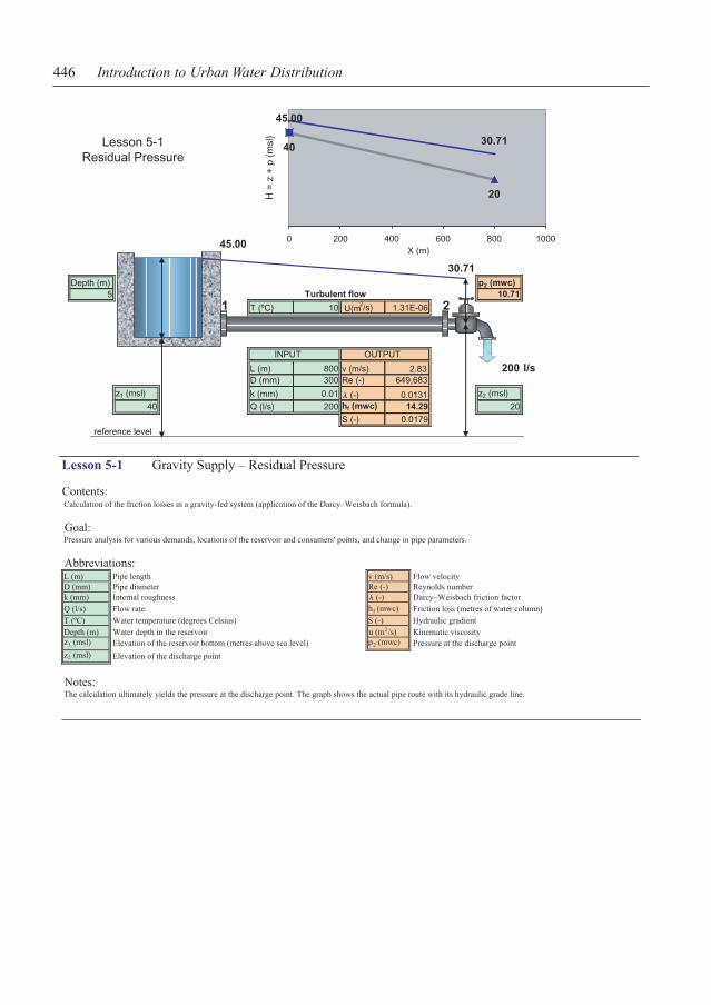
446 Introduction to Urban Water Distribution

45.00

30.71

Depth (m) p2 (mwc)

5 Turbulent flow 10.71

T (ºC) 10 U(m2/s) 1.31E-06

INPUT OUTPUT

L (m) 800 v (m/s) 200 l/sD (mm) 300 Re (-) 649,683

z1 (msl) k (mm) 0.01 l (-) z2 (msl)

40 Q (l/s) 200 hf (mwc) 14.29 20S (-) 0.0179

1 2

reference level

Lesson 5-1Residual Pressure

40

20

45.00

30.71

0 200 400 600 800 1000X (m)

H =

z +

p (

msl

)

0.0131

2.83

Lesson 5-1 Gravity Supply – Residual Pressure

Contents:Calculation of the friction losses in a gravity-fed system (application of the Darcy–Weisbach formula).

Goal:Pressure analysis for various demands, locations of the reservoir and consumers' points, and change in pipe parameters.

Abbreviations:L (m) Pipe length v (m/s) Flow velocityD (mm) Pipe diameter Re (-) Reynolds numberk (mm) Internal roughness l (-) Darcy–Weisbach friction factor

Q (l/s) Flow rate hf (mwc) Friction loss (metres of water column)

T (ºC) Water temperature (degrees Celsius) S (-) Hydraulic gradient

Depth (m) Water depth in the reservoir u (m2/s) Kinematic viscosityz1 (msl) Elevation of the reservoir bottom (metres above sea level) p2 (mwc) Pressure at the discharge point

z2 (msl) Elevation of the discharge point

Notes:The calculation ultimately yields the pressure at the discharge point. The graph shows the actual pipe route with its hydraulic grade line.


65.00

55.00

Depth (m) hf (mwc) 10.00 p2 (mwc)

5 Turbulent flow 35

T (ºC) 10 u (m2/s) 1.31E-06

INPUT OUTPUT

L (m) 1200 S (-) 0.0083 232.53 l/sD (mm) 400 Re (-) 566,388 Iteration complete

z1 (msl) k (mm) 0.3 l(-) 0.0191 z2 (msl)60 v (m/s) 1.85 v (m/s) 1.85 20

Q (l/s) 232.53

1 2

reference level

Lesson 5-2Maximum Capacity

60

20

65.00 55.00

0 200 400 600 800 1000 1200 1400X (m)

H =

z +

p (

msl

)

Lesson 5-2 Gravity Supply – Maximum Capacity

Contents:Hydraulic calculation of a gravity-fed system.

Goal:Determination of the maximum discharge at the required minimum pressure and various positions of the reservoir.

Abbreviations:L (m) Pipe length S (-) Hydraulic gradientD (mm) Pipe diameter Re (-) Reynolds numberk (mm) Internal roughness l (-) Darcy–Weisbach friction factorQ (l/s) Flow rate v (m/s) Calculated flow velocityT (ºC) Water temperature Q (l/s) Flow rate (discharge)Depth (m) Water depth in the reservoir u (m2 /s) Kinematic viscosityz1 (msl) Elevation of the reservoir bottom hf (mwc) Friction loss


v (m/s) Assumed flow velocityp2 (mwc) Pressure required at the discharge point

Notes:The iterative procedure starts by assuming the flow velocity (commonly at 1 m/s) required for determination of the Reynolds number i.e. the friction factor.The velocity calculated afterwards by the Darcy–Weisbach formula serves as an input for the next iteration.The iterative process is achieved by typing the value of the calculated velocity into the cell of the assumed velocity.The message Iteration complete appears once the difference between the velocities in two iterations drops below 0.01 m/s.


55.00

30.00

Depth (m) hf (mwc) 25.00 p2 (mwc)

5 Turbulent flow 10

T (ºC) 10 u(m2/s) 1.31E-06

INPUT OUTPUT

L (m) 500 S (-) 0.0500 100 l/sk (mm) 0.05 D (mm) 193 Iteration complete

z1 (msl) Q (l/s) 100 Re (-) 505,807 z2 (msl)50 v (m/s) 3.43 l(-) 0.0160 20

v (m/s) 3.43

50

20

55.00

30.00

0 100 200 300 400 500 600X (m)

H =

z +

p (

msl

)

1 2

reference level

Lesson 5-3Optimal Diameter

Lesson 5-3 Gravity Supply – Optimal Diameter

Contents:Hydraulic calculation of a gravity-fed system.

Goal:Determination of the optimal pipe diameter at the required minimum pressure and various positions of the reservoir.

Abbreviations:The same as in Lesson 5-2.

Notes:The same iterative procedure is used as in Lesson 5-2, except that the pipe diameter is determined from the assumed/calculated velocity (and specified flow rate).The message Iteration complete appears once the difference between the velocities in two iterations drops below 0.01 m/s.


Depth (m)5

35.00

32.50

p2 (mwc) Turbulent flow 12.50

T (ºC) 15 u(m2/s) 1.14E-06

INPUT OUTPUT

L (m) 500 v (m/s) 1.44 101.5 l/sD (mm) 300 Re (-) 377,920

z1 (msl) k (mm) 0.01 l(-) 0.0142 z2 (msl)

30 Q (l/s) 101.5 hf (mwc) 2.50 20S (-) 0.0050

15.00

12.50

0.02.04.06.08.0

10.012.014.016.018.020.0

0 50 100 150 200Q (l/s)

H =

p2

+ hf

(m

wc)

reference level

Lesson 5-4System Characteristics

z1+ Depth - z2 = p2+ hf

1 2

30

20

35.00 32.50

0 200 400 600X (m)

H =

z +

p (

msl

)

Lesson 5-4 Gravity Supply – System Characteristics

Contents:Friction loss calculation of a gravity-fed system.

Goal:Determination of the system characteristics diagram.

Abbreviations:L (m) Pipe length v (m/s) Flow velocityD (mm) Pipe diameter Re (-) Reynolds numberk (mm) Internal roughness l (-) Darcy–Weisbach friction factor

Q (l/s) Flow rate hf (mwc) Friction loss

T (ºC) Water temperature S (-) Hydraulic gradient

Depth (m) Water depth in the reservoir p2 (mwc) Pressure at the discharge pointz1 (msl) Elevation of the reservoir bottom u (m2/s) Kinematic viscosity


Notes:The friction loss is calculated for the flow range 0–1.5Q (specified) and the results are plotted on the graph.The point on the graph shows the upstream head required to maintain the downstream pressure for flow Q.That head equals the elevation difference between the water surface in the reservoir and the discharge point.The static head equals the downstream pressure, which fluctuates when the system parameters are modified.


Err (msl) 0.00Iteration complete

Q2 (l/s) H2 (msl)

60 23.03

z2 (msl) p2 (mwc)20 3.03

Turbulent flow Turbulent flow

T (ºC) 10 u(m2/s) 1.31E-06

60 l/s

H1 (msl) INPUT 1-2 OUTPUT 1-2 INPUT 3-2 OUTPUT 3-2 H3 (msl)

25.00 L (m) 500 v (m/s) 0.95 L (m) 500 v (m/s) 0.95 25.00Depth (m) D (mm) 200 Re (-) 146,179 D (mm) 200 Re (-) 146,179 Depth (m)

5 k (mm) 0.01 l(-) 0.0169 k (mm) 0.01 l(-) 0.0169 5z1 (msl) Q (l/s) 30 hf (mwc) 1.97 Q (l/s) 30 hf (mwc) 1.97 z3 (msl)

20 S (-) 0.0039 S (-) 0.0039 20

1

reference level

Lesson 5-5aSupply From Two Sides

2

3

H1 - hf1-2 = H2 = H3 - hf3-220 20 20

25.00 23.03 25.00

0 200 400 600 800 1000 1200X (m)

H =

z +

p (

msl

)

Lesson 5-5a Gravity Supply – Supply from Two Sides

Contents:Friction loss calculation of a gravity system fed from two sides.

Goal:To calculate the contribution from each source, based on various locations of the supply and discharge points, and changes in pipe parameters.

Abbreviations:L (m) Pipe length v (m/s) Flow velocityD (mm) Pipe diameter Re (-) Reynolds numberk (mm) Internal roughness l (-) Darcy–Weisbach friction factorQ2 (l/s) Discharge hf (mwc) Friction loss

Q (l/s) Flow rate in pipe 1-2 S (-) Hydraulic gradientT (ºC) Water temperature Q (l/s) Flow rate in pipe 3-2z1,3 (msl) Elevation of the reservoir bottoms u (m2/s) Kinematic viscosity

z2 (msl) Elevation of the discharge point H1-3 (msl) Piezometric heads

Depth (m) Water depth in the reservoirs Err (msl) The difference in H2 calculated from both sides

Notes:The process of trial and error consists of altering the flow in pipe 1-2, which has implications for the head-losses in both pipes.The process ends when the difference in H2 calculated from the left and right side drops below 0.01 msl and the message Iteration complete appears.

Negative values for pipe flows indicate a change of direction i.e. the water that is flowing to the reservoir.


z2 (msl) p2 (mwc)12 8


T (ºC) 10 u (m2/s) 1.31E-06

84.02 l/s

H1 (msl) INPUT 1-2 OUTPUT 1-2 INPUT 3-2 OUTPUT 3-2 H3 (msl)

25.00 L (m) 500 S (-) 0.0100 L (m) 500 S (-) 0.0200 30.00Depth (m) D (mm) 200 Re (-) 243,394 D (mm) 150 Re (-) 220,432 Depth (m)

5 k (mm) 0.01 l(-) 0.0155 k (mm) 0.01 l(-) 0.0159 5z1 (msl) v (m/s) 1.59 v (m/s) 1.59 v (m/s) 1.92 v (m/s) 1.92 z3 (msl)

20 Iteration complete Q (l/s) 50.01 Iteration complete Q (l/s) 34.01 25

1

reference level

Lesson 5-5bSupply From Two SidesSystem Characteristics

2

3

13.00

18.00

8.00

0.05.0

10.015.020.025.030.035.040.0

0 20 40 60 80Q (l/s)

H =

p2

+ hf

(m

wc)

Lesson 5-5b Gravity Supply – Supply from Two Sides, System Characteristics

Contents:Friction loss calculation of a gravity system fed from two sides.

Goal:To calculate the contribution from each source, based on various locations of the supply and discharge points, and changes in pipe parameters.

Abbreviations:The same as in Lesson 5-5a.

Notes:The contribution from each source to the discharge is analysed by constructing pipe characteristics for both pipes.The same procedure as in Lesson 5-4 is applied here.

20

12

25

25.00

20.00

30.00

0 500 1000 1500X (m)

H =

z +

p (

msl

)


120.00

H1 (msl) 90.54

40

p2 (mwc) Turbulent flow 40.54

T (ºC) 10 u (m2/s) 1.31E-06

INPUT OUTPUT

L (m) 1000 v (m/s) 5.09 1000 l/s

Qd (l/s) D (mm) 500 Re (-) 1,949,049

1000 k (mm) 0.01 l(-) 0.0111 z2 (msl)

Hd (mwc) Qp (l/s) 1000 hf (mwc) 29.46 50

80 Eff. (%) 65% P (kW) 1207.38

80.00

0.0

20.0

40.0

60.0

80.0

100.0

120.0

0 500 1000 1500 2000Qp (l/s)

Hp

(mw

c)

1

2

reference level

Lesson 6-1ResidualPressure

120.00

90.54

4050

0 200 400 600 800 1000 1200X (m)

H =

z +

p (

msl

)

Lesson 6-1 Pumped Supply – Residual Pressure

Contents:Calculation of the friction losses in a pumped system.

Goal:Calculation of pumping heads and friction losses in a pumped system.

Abbreviations:L (m) Pipe length v (m/s) Flow velocityD (mm) Pipe diameter Re (-) Reynolds numberk (mm) Internal roughness l(-) Darcy–Weisbach friction factorQp (l/s) Pumped discharge hf (mwc) Friction loss

Eff. (%) Pump efficiency at Qp P (k W) Pump power consumption at QpQd (l/s) Pump duty flow p2 (mwc) Pressure at the discharge pointHd (mwc) Pump duty head u (m2/s) Kinematic viscosity

H1 (msl) Piezometric head at the suction side of the pump


T (ºC) Water temperature

Notes:The pump curve is approximated by the formula Hp= c–aQp

b, where c = 4Hd/3, b = 2 and a = Hd/3/Qd2.

The pump graph is plotted for the Qp range between 0 and 1.8Qd. The duty head and duty flow indicate the working point of the maximum pump efficiency.

The pump raises head H1 to head H1+Hp from where the pipe friction loss is going to be deducted.

The calculation ultimately yields the pressure at the discharge point. The graph shows the actual pipe route with its hydraulic grade line.


74.19

H1 (msl) 55.00

65 Optimal Qp (D)

Hw (mwc) 0.00 Pw (kW) 0.01 p2 (mwc) p2 (mwc)

Turbulent flow 35 35.00

T (ºC) 10 u (m2/s) 1.31E-06

INPUT OUTPUT

L (m) 1200 v (m/s) 2.58 323.78 l/s

Qd (l/s) D (mm) 400 Re (-) 788,829

200 k (mm) 0.3 l(-) 0.0189 z2 (msl)

Hd (mwc) Qp (l/s) 323.78 hf (mwc) 19.19 20

20 Eff. (%) 65% P (kW) 44.93

9.19

9.19

-10.00

-15.0-10.0-5.0

0.05.0

10.015.0

20.025.030.0

0 100 200 300 400

Qp (l/s)

Hp

(mw

c)

1

2

reference level

Lesson 6-2MaximumCapacity

(Optimal D)

74.1955.00

65

20

0 500 1000 1500X (m)

H =

z +

p (

msl

)

Lesson 6-2 Pumped Supply – Maximum Capacity/Optimal Diameter

Contents:Calculation of pumping heads and friction losses in a pumped system.

Goal:Relation between the pump and system characteristics.

Abbreviations:L (m) Pipe length v (m/s) Flow velocityD (mm) Pipe diameter Re (-) Reynolds numberk (mm) Internal roughness l (-) Darcy–Weisbach friction factorQp (l/s) Pumped discharge hf (mwc) Friction loss

Eff. (%) Pump efficiency at Qp P (k W) Pump power consumption at Qp

Qd (l/s) Pump duty flow p2 (mwc) Actual pressure at the discharge point

Hd (mwc) Pump duty head Hw (mwc) Excessive pumping head

H1 (msl) Piezometric head at the suction side of the pump P w (kW) Excessive pumping powerz2 (msl) Elevation of the discharge point u (m2/s) Kinematic viscosity

p2 (mwc) Minimum pressure required at the discharge point


Notes:The pump curve is plotted in the same way as in Lesson 6-1. The system characteristics curve is plotted for the same range of flows.The diagram shows the difference between the pumping head and the head required to deliver the minimum pressure at the discharge point.The optimal working point is in the intersection between the pump- and system characteristics curves (Hw= 0).


Hrequired 66.30

Hp(A) 52.50

Hp(B) 20.27

Hp(A+B) 94.03

124.03

H1 (msl) 87.73

30 Increase Qp (reduce D)!



T (ºC) 10 u (m2/s) 1.31E-06

INPUT OUTPUT

L (m) 1000 v (m/s) 6.37 1800 l/s

Pump A Pump B D (mm) 600 Re (-) 2,923,573

Qd (l/s) 1200 1000 k (mm) 0.01 l(-) 0.0105 z2 (msl)Hd (mwc) 90 80 Qp (l/s) 1800 hf (mwc) 36.30 40

On (=1) 1 1 Eff. (%) 65% P (kW) 1426.22

Lesson 6-3Pumps in Parallel

30.00

0.0

50.0

100.0

150.0

200.0

250.0

0 1000 2000 3000 4000 5000Qp (l/s)

Hp

(mw

c)

1

2

reference level

124.03

87.73

3040

0 200 400 600 800 1000 1200X (m)

H =

z +

p (

msl

)

Hp = HpA = HpB

Qp = QpA + QpB

Lesson 6-3 Pumped Supply – Pumps in Parallel

Contents:Calculation of pumping heads and friction losses for parallel arrangement of the pumps.

Goal:Relation between the pump- and system characteristics for various pump sizes and operational modes.

Abbreviations:L (m) Pipe length v (m/s) Flow velocityD (mm) Pipe diameter Re (-) Reynolds numberk (mm) Internal roughness l (-) Darcy–Weisbach friction factorQp (l/s) Pumped discharge h f (mwc) Friction loss

Eff. (%) Efficiency at Qp P (k W) Pump power consumption at Qp

Qd (l/s) Pump duty flow (A,B) p2 (mwc) Actual pressure at the discharge point

Hd (mwc) Pump duty head (A,B) Hw (mwc) Excessive pumping head

On (=1) The pump is 'off' unless the cell input =1 P w (kW) Excessive pumping power

H1 (msl) Piezometric head at the suction side of the pump u(m 2/s) Kinematic viscosity

z2 (msl) Elevation of the discharge point Hrequired Minimum required head at Qp

p2 (mwc) Minimum pressure required at the discharge point Hp(A) Pumping head A at Qp

T (ºC) Water temperature Hp(B) Pumping head B at Qp

Hp(A+B) Head of pumps A & B both in operation at Qp

Notes:The pump and system characteristics curves are plotted in the same way as in Lesson 6-2.The diagram shows the difference between the pumping head and the head required to deliver the minimum pressure at the discharge pointin all three cases: single operation of pumps A & B and their joint operation. The hydraulic grade line on the graph is plotted for actual operation of the pumps.


Hrequired 96.89

Hp(A) 68.27

Hp(B) 35.00

Hp(A+B) 103.27

133.27

H1 (msl) 116.37

30 Increase Qp (reduce D)!



T (ºC) 10 u (m2/s) 1.31E-06

INPUT OUTPUT

L (m) 1000 v (m/s) 4.24 1200 l/s

Pump A Pump B D (mm) 600 Re (-) 1,949,049

Qd (l/s) 1000 800 k (mm) 0.01 l(-) 0.0110 z2 (msl)Hd (mwc) 80 60 Qp (l/s) 1200 hf (mwc) 16.89 90

On (=1) 1 1 Eff. (%) 65% P (kW) 1236.36

Lesson 6-4Pumps in Series

80.00

0.020.040.060.080.0

100.0120.0140.0160.0180.0200.0

0 500 1000 1500 2000Qp (l/s)

Hp

(mw

c)

1

2

reference level

133.27 116.37

90

30

0 200 400 600 800 1000 1200X (m)

H =

z +

p (

msl

)

Hp = HpA + HpB

Qp = QpA = QpB

Lesson 6-4 Pumped Supply – Pumps in Series

Contents:Calculation of pumping heads and friction losses for serial arrangement of pumps.

Goal:Relation between the pump- and system characteristics curves for various pump sizes and operational modes.

Abbreviations:The same as in Lesson 6-3.

Notes:The same as in Lesson 6-3.


75.70

H1 (msl) 70.05

30 Reduce pump speed (drpm)!



T (ºC) 10 u (m2/s) 1.31E-06

INPUT OUTPUT

L (m) 1000 v (m/s) 2.72 1200 l/sD (mm) 750 Re (-) 1,559,239

Qd (l/s) 1000 k (mm) 0.01 l(-) 0.0113 z2 (msl)Hd (mwc) 60 Qp (l/s) 1200 hf (mwc) 5.64 40

drpm (%) -3.5 Eff. (%) 65 P (kW) 927.27

Lesson 6-5Variable Speed

Pump

45.64

45.70

40.00

0.010.020.030.040.050.060.070.080.090.0

0 500 1000 1500 2000Qp (l/s)

Hp

(mw

c)

1

2

reference level

75.70 70.05

40

30

0 200 400 600 800 1000 1200X (m)

H =

z +

p (

msl

)

Q2/Q1 = n2/n1

H2/H1 = (n2/n1)2

Lesson 6-5 Pumped Supply – Variable Speed Pump

Contents:Calculation of pumping heads and friction losses in a system with variable speed pump.

Goal:Analysis of effects caused by modification of the pump speed.

Abbreviations:L (m) Pipe length v (m/s) Flow velocityD (mm) Pipe diameter Re (-) Reynolds numberk (mm) Internal roughness l (-) Darcy–Weisbach friction factorQp (l/s) Pumped discharge hf (mwc) Friction loss

Eff. (%) Pump efficiency at Qp P (k W) Pump power consumption at Qp

Qd (l/s) Pump duty flow p2 (mwc) Actual pressure at the discharge point

Hd (mwc) Pump duty head Hw (mwc) Excessive pumping head

drpm (%) Pump speed increase/decrease P w (kW) Excessive pumping powerH1 (msl) Piezometric head at the suction side of the pump u (m2/s) Kinematic viscosity


p2 (mwc) Minimum pressure required at the discharge point


Notes:The diagram shows the difference in pumping heads between the pump curve at the original and modified speeds.


T (ºC) 10

u (m2/s) 1.31E-06 79.00

54.19

25.00p3 (mwc) p3 (mwc)

Depth (m) 19.00 Turbulent flow 30 34.195 Qd (l/s) 1000

z1 (msl) Hd (mwc) 60 Hw (mwc) 4.19

20 z2 (msl) z3 (msl) Pw (kW) 63.31

10 20

Turbulent flow 1000 l/s

INPUT 1-2 OUTPUT 1-2 INPUT 2-3 OUTPUT 2-3 Increase Qp (reduce D)!

L (m) 500 v (m/s) 3.54 L (m) 500 v (m/s) 6.29 Qp (l/s) 1000D (mm) 600 Re (-) 1,624,207 D (mm) 450 Re (-) 2,165,610 Eff. (%) 65%

k (mm) 0.01 l(-) 0.0113 k (mm) 0.01 l(-) 0.0111 Hp (mwc) 60.00

hf (mwc) 6.00 hf (mwc) 24.81 P (kW) 905.54

55.81

60.00

31.00

0.0

20.0

40.0

60.0

80.0

100.0

120.0

0 500 1000 1500 2000Qp (l/s)

Hp

(mw

c)

Lesson 7-1TankPump

Consumer

1

reference level

3

20

10

20

25.0019.00

79.00

54.19

0 200 400 600 800 1000 1200X (m)

H =

z +

p (

msl

)

2

Lesson 7-1 Combined Supply – Tank, Pump, Consumer

Contents:Calculation of pumping heads and friction losses in a system combining gravity and pumped supply.

Goal:Determination of residual pressure/maximum capacity/optimal diameters for various scenarios.

Abbreviations:The same as in Lessons 5 and 6.

Remarks:The system characteristics curve in the diagram is plotted for the pipe on the pressure side of the pump.


Hp (mwc) 41.19

P (kW) 938.15Optimal Qp (D)

Hw (mwc) 0.01Pw (kW) 0.17

81.19

T (ºC) 10

u (m2/s) 1.31E-06H1 (msl)

40 Depth (m) 5 42.17z2 (msl) 65

p3 (mwc)12.17


INPUT 1-2 OUTPUT 1-2 INPUT 2-3 OUTPUT 2-3

L (m) 500 v (m/s) 4.93 L (m) 500 v (m/s) 7.13 1400 l/sQd (l/s) 1000 D (mm) 600 Re (-) 2,262,521 D (mm) 500 Re (-) 2,728,668

Hd (mwc) 60 k (mm) 0.01 l (-) 0.0108 k (mm) 0.01 l(-) 0.0107 z3 (msl)

Eff. (%) 60% Qp (l/s) 1393 hf (mwc) 11.18 Q (l/s) 1400 hf (mwc) 27.83 30

Lesson 7-2PumpTank

Consumer

1

reference level

3

40

65

30

81.19 70.00

42.17

0 200 400 600 800 1000 1200X (m)

H =

z +

p (

msl

)

2

41.18

41.19

30.00

0.010.020.030.040.050.060.070.080.090.0

0 500 1000 1500 2000Qp (l/s)

Hp

(mw

c)

Lesson 7-2 Combined Supply – Pump, Tank, Consumer

Contents:Calculation of pumping heads and friction losses in a system combining the gravity and pumped supply.



Remarks:The system characteristics in the diagram is plotted for the pipe on the upstream side of the reservoir.The static head of that pipe is equal to the difference between the water levels in the two reservoirs.The system is hydraulically disconnected and the maximum discharge capacity is dependant on the gravity part only.


Lesson 7-3 Combined Supply – Pump, Consumer, Tank

Contents:Calculation of pumping heads and friction losses in a system combining gravity and pumped supply.



Notes:For a specified pumping flow, the contribution from the reservoir will be calculated through an iteration of velocities in pipe 3-2.A negative value of the hydraulic gradient (S) in pipe 3-2 indicates a reversed flow direction i.e. filling of the reservoir (night regime).By the alternative approach (see the table 'ALTERNATIVE APPROACH') the contribution from both supplying points will be determined for specified demand.This is reached through a process of trial and error, with 'Err' indicating the difference in head H2 calculated from both sides.

The pump is switched off by leaving the cells for Hd or/and Qd empty.

Hp (mwc) 35.00

P (kW) 858.38

Increase Qp (reduce D)!

Hw (mwc) 5.67Pw (kW) 139.14

75.00

T (ºC) 10

(m 2/s) 1.31E-06 75.00

60.67

H1 (msl) 40 Depth (m)z2 (msl) p2 (mwc) p2 (mwc) Q2 (l/s) 5

30 25 30.67 1524.94 z3 (msl)

70


1524.9 l/s ALTERNATIVE APPROACH

INPUT 1-2 OUTPUT 1-2 INPUT 3-2 OUTPUT 3-2 Q2 (l/s) 1525

L (m) 500 v (m/s) 3.90 L (m) 500 S (-) 0.0287 Qp (l/s) 1500

Qd (l/s) 1000 D (mm) 700 Re (-) 2,088,266 D (mm) 150 Re (-) 161,880 Q3-2 (l/s) 25.00

Hd (mwc) 60 k (mm) 2 l(-) 0.0259 k (mm) 2 l(-) 0.0423 p2 (mwc) 30.67

Eff. (%) 60% Qp (l/s) 1500 hf (mwc) 14.33 v (m/s) 1.41 v (m/s) 1.41 Err (mwc) -0.06

Iteration complete Q (l/s) 24.94 Increase Qp!

Lesson 7-3Pump

ConsumerTank

1

reference level

3

40

30

70

75.00 60.67 75.00

0 200 400 600 800 1000 1200X (m)

H =

z +

p (

msl

)

2

29.33

35.00

15.00

0.010.0

20.030.040.0

50.060.070.0

80.090.0

0 500 1000 1500 2000Qp (l/s)

Hp

(mw

c)


Hst1-2 20.00

Hst2-3 25.78

T (ºC) 10 u (m2/s) 1.31E-06

105.4284.64

H1 (msl) 62.67 p3 (mwc) p3 (mwc) Pump 1 Pump 2

20 54.22 30 34.64 Qd (l/s) 1000 1000

Turbulent flow Hd (mwc) 50 60z (msl) 20 40

Turbulent flow Qp (l/s) 1200 1200

z3 (msl) Increase Qp (reduce D)!

50 1200 l/s

Eff. (%) 65% 65Hrequired 28.45 46.56

INPUT 1-2 OUTPUT 1-2 INPUT 2-3 OUTPUT 2-3 Hp (mwc) 42.67 51.20

L (m) 500 v (m/s) 4.24 L (m) 500 v (m/s) 6.11 P (kW) 772.73 927.27D (mm) 600 Re (-) 1,949,049 D (mm) 500 Re (-) 2,338,858 Hw (mwc) 14.22 4.64

k (mm) 0.01 l(-) 0.0110 k (mm) 0.01 l(-) 0.0109 Pw (kW) 257.53 83.96

hf (mwc) 8.45 hf (mwc) 20.78

Lesson 7-4Zoned Supply

1

reference level

3

20

4050

62.6754.22

105.4284.64

0 200 400 600 800 1000 1200X (m)

H =

z +

p (

msl

)

2

0.010.020.030.040.050.060.070.080.090.0

0 500 1000 1500 2000Qp (l/s)

Hp

(mw

c)

Lesson 7-4 Combined Supply – Zoned Supply

Contents:Calculation of pumping heads and friction losses in a system combining the gravity and pumped supply.

Goal:Determination of residual pressure/maximum capacity/optimal diameters for booster pumping.

Abbreviations:The same as in Lessons 5 and 6. In addition, ‘Hst1-2’ and ‘Hst3-2’ indicate the static heads of pipes 1-2 and 3-2 respectively.

Remarks:The diagram shows the pump characteristics of each pump with its corresponding pipe characteristics.The optimal working point for specified discharge and minimum downstream pressure is in the intersection of the red coloured curves.The green coloured curves are monitored for avoiding under-pressure in the part of the system between the two pumps.The pumps are switched off by leaving the cells for Hd or/and Qd empty.


VOLUME m3 litre ft3 gal galUS Hour Demand1 2 3 4 5 l/s m3/h

m3 1 1000 35.315 219.97 264.19 1 989.6 3562.56litre 0.0010 1 0.0353 0.2200 0.2642 2 945.9 3405.24ft3 0.0283 28.317 1 6.2288 7.4811 3 902.2 3247.92

Flow Rate Units gal 0.0045 4.5461 0.1605 1 1.2011 4 727.6 2619.36100 l/s galUS 0.0038 3.7851 0.1337 0.8326 1 5 844 3038.4

6 1164.2 4191.127 1571.7 5658.12

TIME sec min hour day 8 1600.8 5762.881 2 3 4 9 1775.4 6391.44

sec 1 0.0167 2.8E-04 1.2E-05 10 1964.6 7072.56min 60 1 0.0167 6.9E-04 11 2066.4 7439.04

Units Flow Rate hour 3600 60 1 0.0417 12 2110.1 7596.36m3/h 360 day 86400 1440 24 1 13 1600.8 5762.88

14 1309.7 4714.9215 1091.4 3929.04

FLOW m3/s l/s m3/h Ml/d ft3/s gpm mgd gpmUS mgdUS 16 945.9 3405.241 2 3 4 5 6 7 8 9 17 1062.3 3824.28

m3/s 1 1000 3600 86.4 35.315 13198 19.005 15852 22.826 18 1455.2 5238.72l/s 0.001 1 3.6 0.0864 0.0353 13.198 0.019 15.852 0.0228 19 1746.3 6286.68

m3/h 2.8E-04 0.2778 1 0.0240 0.0098 3.6661 0.005 4.4032 0.0063 20 2139.2 7701.12Ml/d 0.0116 11.574 41.667 1 0.4087 152.76 0.220 183.47 0.2642 21 2110.1 7596.36ft3/s 0.0283 28.317 101.94 2.4466 1 373.73 0.538 448.87 0.6464 22 2037.3 7334.28gpm 7.6E-05 0.0758 0.2728 0.0065 0.0027 1 0.001 1.2011 0.0017 23 1746.3 6286.68mgd 0.0526 52.617 189.42 4.5461 1.8581 694.44 1 834.06 1.2011 24 1018.7 3667.32

gpmUS 6.3E-05 0.0631 0.2271 0.0055 0.0022 0.8326 0.0012 1 0.0014 Total 34,925.7 125,733mgdUS 0.0438 43.809 157.71 3.7851 1.5471 578.20 0.8326 694.44 1 Average 1455.24 5238.86

Lesson 8-1Flow Conversion

converted into:

Lesson 8-1 Flow Conversion

Contents:Comparison of the flow units.

Goal:Conversion of the common flow units.

Abbreviations:m3/s cubic metre per secondl/s litre per secondm3/h cubic metre per hourMl/d mega-litre per day

ft3/s cubic feet per secondgpm gallon per minute (Imperial)mgd mega-gallon per day (Imperial)gpmUS gallon per minute (US)mgdUS mega-gallon per day (US)

Notes:Both individual values and the series of 24 hourly flows are converted from/to the units specified in the table (by typing).


Lesson 8-2 Diurnal Demand

Contents:Diurnal demand diagram.

Goal:Determination of hourly peak factors.

Notes:The peak factors are calculated as ratios between the actual and average hourly demand.

Hour Demand Peak

(m3/h) Factor

1 989.60 0.6802 945.90 0.6503 902.20 0.6204 727.60 0.5005 844.00 0.5806 1164.20 0.8007 1571.70 1.0808 1600.80 1.1009 1775.40 1.22010 1964.60 1.35011 2066.40 1.42012 2110.10 1.45013 1600.80 1.10014 1309.70 0.90015 1091.40 0.75016 945.90 0.65017 1062.30 0.73018 1455.20 1.00019 1746.30 1.20020 2139.20 1.470

Hour Demand Peak 21 2110.10 1.450(m3/h) Factor 22 2037.30 1.400

Maximum 20 2139.20 1.47 23 1746.30 1.200Minimum 4 727.60 0.50 24 1018.70 0.700

Total 34,925.70 24.00Average 1455.24 1.000

Lesson 8-2Diurnal Demand

0

500

1000

1500

2000

2500

1 5 9 13 17 210.0

0.2

0.4

0.6

0.8

1.0

1.2

1.4

1.6


Hour Cat.1 Peak Cat.2 Peak Demand Cum.

(m3/h) Fact.1 (m3/h) Fact.2 (m3/h) Peak F.

1 989.60 0.680 579.00 0.389 1568.60 0.5332 945.90 0.650 523.00 0.351 1468.90 0.4993 902.20 0.620 644.00 0.432 1546.20 0.5254 727.60 0.500 835.00 0.561 1562.60 0.5315 844.00 0.580 1650.00 1.108 2494.00 0.8476 1164.20 0.800 1812.00 1.217 2976.20 1.0117 1571.70 1.080 1960.00 1.316 3531.70 1.2008 1600.80 1.100 1992.00 1.338 3592.80 1.2209 1775.40 1.220 1936.00 1.300 3711.40 1.26110 1964.60 1.350 1887.00 1.267 3851.60 1.30811 2066.40 1.420 1821.00 1.223 3887.40 1.32012 2110.10 1.450 1811.00 1.216 3921.10 1.33213 1600.80 1.100 1837.00 1.234 3437.80 1.16814 1309.70 0.900 1884.00 1.265 3193.70 1.08515 1091.40 0.750 2011.00 1.351 3102.40 1.05416 945.90 0.650 2144.00 1.440 3089.90 1.04917 1062.30 0.730 2187.00 1.469 3249.30 1.10418 1455.20 1.000 2132.00 1.432 3587.20 1.21819 1746.30 1.200 1932.00 1.297 3678.30 1.24920 2139.20 1.470 1218.00 0.818 3357.20 1.140

Peak Factors 1 Peak Factors 2 Cum. Peak Factors 21 2110.10 1.450 898.00 0.603 3008.10 1.022Maximum 1.470 Maximum 1.469 Maximum 1.332 22 2037.30 1.400 786.00 0.528 2823.30 0.959at hour 20 at hour 17 at hour 12 23 1746.30 1.200 657.00 0.441 2403.30 0.816Minimum 0.500 Minimum 0.351 Minimum 0.499 24 1018.70 0.700 601.00 0.404 1619.70 0.550at hour 4 at hour 2 at hour 2 Total 34,925.70 24.00 35,737.00 24.00 70,662.70 24.00

Average 1455.24 1.000 1489.04 1.000 2944.28 1.000

Lesson 8-3Demand Categories

0.0

0.2

0.4

0.6

0.8

1.0

1.2

1.4

1.6

1 5 9 13 17 21

Lesson 8-3 Demand Categories


Goal:Determination of hourly peak factors for various demand categories and the overall demand pattern.

Notes:The peak factors of the cumulative demand diagram have no direct relation to the peak factors of the categories composing this diagram.


D/M Sun Oct Average Week PeakHour Demand Peak Demand Factors

(m3/h) Factors (m3/h) Mon 1.1401 433.00 0.302 529.99 Tue 1.0102 562.00 0.391 687.88 Wed 0.9503 644.00 0.449 788.25 Thu 0.9804 835.00 0.582 1022.03 Fri 1.0405 1450.00 1.010 1774.79 Sat 1.0206 1644.00 1.145 2012.24 Sun 0.8607 1856.00 1.293 2271.73 Average 1.0008 1922.00 1.339 2352.519 1936.00 1.349 2369.6510 1887.00 1.314 2309.67 Year Peak11 1721.00 1.199 2106.49 Factors12 1712.00 1.193 2095.47 Jan 0.96013 1634.00 1.138 2000.00 Feb 0.97014 1656.00 1.154 2026.93 Mar 1.01015 1789.00 1.246 2189.72 Apr 1.03016 1925.00 1.341 2356.18 May 1.04017 2087.00 1.454 2554.47 Jun 1.05018 2055.00 1.431 2515.30 Jul 1.04019 1944.00 1.354 2379.44 Aug 1.03020 1453.00 1.012 1778.46 Sep 0.990

Hour Demand Day (m3/h) Peak 21 1218.00 0.848 1490.82 Oct 0.950Current Average Factors 22 813.00 0.566 995.10 Nov 0.960

Maximum 17 2087.00 2554.47 1.454 23 676.00 0.471 827.42 Dec 0.970Minimum 1 433.00 529.99 0.302 24 602.00 0.419 736.84 Average 1.000

Average 1435.58 1.000 1757.14

Lesson 8-4Seasonal Variations

0

500

1000

1500

2000

2500

3000

1 5 9 13 17 21

Lesson 8-4 Seasonal Variations


Goal:Comparison of the diurnal demand patterns for various periods of the week/year.

Abbreviations:D/M Day/Month

Notes:Recalculation of the hourly demand and corresponding peak factors takes place by typing the day and month from the tables for weekly and monthly peak factors.The last peak factor value specified in the weekly and annual table is calculated so that the value can fill up to 7 and 12 respectively,which generate the average equal to 1.0.


Hour Peak Water Quantities (m3/h)Factors Qwc Qwl Qd

1 0.680 4250.00 1821.43 6071.432 0.650 4062.50 1741.07 5803.573 0.620 3875.00 1660.71 5535.714 0.500 3125.00 1339.29 4464.295 0.580 3625.00 1553.57 5178.576 0.800 5000.00 2142.86 7142.867 1.080 6750.00 2892.86 9642.868 1.100 6875.00 2946.43 9821.439 1.220 7625.00 3267.86 10,892.8610 1.350 8437.50 3616.07 12,053.5711 1.420 8875.00 3803.57 12,678.5712 1.450 9062.50 3883.93 12,946.4313 1.100 6875.00 2946.43 9821.4314 0.900 5625.00 2410.71 8035.7115 0.750 4687.50 2008.93 6696.4316 0.650 4062.50 1741.07 5803.5717 0.730 4562.50 1955.36 6517.8618 1.000 6250.00 2678.57 8928.5719 1.200 7500.00 3214.29 10,714.2920 1.470 9187.50 3937.50 13,125.0021 1.450 9062.50 3883.93 12,946.43

Number of q Qwc, av g Leakage Equation Qd, av g 22 1.400 8750.00 3750.00 12,500.00

consum. (l/c/d) (m3/h) (%) 2.1/2.6 (m3/h) 23 1.200 7500.00 3214.29 10,714.291,000,000 150 6250.00 30% 2.1 8928.57 24 0.700 4375.00 1875.00 6250.00

Average 1.000 6250.00 2678.57 8928.57

Lesson 8-5Demand Calculation

0

2000

4000

6000

8000

10,000

12,000

14,000

1 5 9 13 17 21

Lesson 8-5 Demand Calculation


Goal:Calculation of the leakage component for specified diurnal pattern and leakage percentage.

Abbreviations:Number of Number of consumers in the area Leakage Leakage expressed as a percentage of water productionconsum. (%)

q Specific consumption (unit per capita consumption) Equation Equation used for the demand calculation, as discussed in Chapter 2(l/c/d) 2.1/2.6

Qwc, av g Average consumption Qd, av g Average demand

(m3/h) (m3/h)

Qwc Qwl Qd Hourly water consumption, water leakage and water demand, respectively

Notes:The demand is calculated in two ways: a) with the leakage proportional to the peak factor values (Equation 2.1 in Chapter 2 of the book), and b) with constant leakage, independent from the peak factors (Equation 2.6). Both approaches yield the same average demand but the range of the hourly flows will be wider in the first approach. This adds a safety factor to the result although it reflects the reality to a lesser extent. The last hourly peak factor value specified in the table is calculated so that the value can fill up to 24, which generates the average equal to 1.0.


Number of q Leakage Qd, av g Hour Peak Demand Day (m3/h)

consum. (l/c/d) (%) (m3/h) Factors Avg. Max. Min.

1,000,000 150 30% 8928.57 1 0.680 6071.43 7267.50 4960.362 0.650 5803.57 6946.88 4741.523 0.620 5535.71 6626.25 4522.684 0.500 4464.29 5343.75 3647.325 0.580 5178.57 6198.75 4230.896 0.800 7142.86 8550.00 5835.717 1.080 9642.86 11,542.50 7878.218 1.100 9821.43 11,756.25 8024.119 1.220 10,892.86 13,038.75 8899.4610 1.350 12,053.57 14,428.13 9847.7711 1.420 12,678.57 15,176.25 10,358.3912 1.450 12,946.43 15,496.88 10,577.2313 1.100 9821.43 11,756.25 8024.1114 0.900 8035.71 9618.75 6565.1815 0.750 6696.43 8015.63 5470.9816 0.650 5803.57 6946.88 4741.5217 0.730 6517.86 7801.88 5325.0918 1.000 8928.57 10,687.50 7294.6419 1.200 10,714.29 12,825.00 8753.5720 1.470 13,125.00 15,710.63 10,723.1321 1.450 12,946.43 15,496.88 10,577.23

Variation Peak Factors Hour Qpeak 22 1.400 12,500.00 14,962.50 10,212.50

Weekday Month Overall (m3/h) 23 1.200 10,714.29 12,825.00 8753.57Maximum 1.140 1.050 1.197 20 15,710.63 24 0.700 6250.00 7481.25 5106.25Minimum 0.860 0.950 0.817 4 3647.32 Average 1.000 8928.57 10,687.50 7294.64

Lesson 8-6Design Demand

0

2000

4000

6000

8000

10,000

12,000

14,000

16,000

18,000

1 5 9 13 17 21

Lesson 8-6 Design Demand


Goal:Establishing the range of demands/peak factors that can occur during the year.

Abbreviations:Qpeak Absolute maximum and minimum peak demand

(m3/h)

Notes:Weekly and monthly factors compose the average consumption during the maximum/minimum consumption day. Maximum/minimum hourly peak factorsin combination with the seasonal factors give the range of demands in the system between the maximum consumption hour of the maximum consumption day andthe minimum consumption hour of the minimum consumption day.The leakage component is calculated applying the first approach from the previous lesson (by using Equation 2.1).The last hourly peak factor value specified in the table is calculated so that the value can fill up to 24, which generates the average equal to 1.0.


CONSUMPTION CATEGORIESA B C D E F G H

CATEGORIES q (m3/d/ha) District 1 p (%) 37% 23% 10% 0% 4% 0% 0% 26%A Residential area, apartments 90 Area 1 (ha) c (%) 100% 100% 100% 0% 100% 0% 0% 40%B Individual houses 55 250 Ac(ha) 92.5 57.5 25 0 10 0 0 26

C Shopping area 125 District 2 p (%) 20% 5% 28% 11% 12% 0% 5% 19%D Offices 80 Area 2 (ha) c (%) 100% 100% 95% 100% 100% 0% 100% 80%E Schools, Universities 100 185 Ac(ha) 37 9.25 49.21 20.35 22.2 0 9.25 28.12

F Hospitals 160 District 3 p (%) 10% 18% 3% 0% 0% 42% 0% 27%G Hotels 150 Area 3 (ha) c (%) 100% 100% 100% 0% 0% 100% 0% 35%H Public green areas 15 57 Ac(ha) 5.7 10.26 1.71 0 0 23.94 0 5.3865

District 4 p (%) 25% 28% 20% 2% 15% 0% 0% 10%Area 4 (ha) c (%) 100% 100% 95% 100% 100% 0% 0% 36%

88 Ac(ha) 22 24.64 16.72 1.76 13.2 0 0 3.168

Q (m3/h) Inhab. Q(l/c/d) District 5 p (%) 50% 0% 11% 0% 10% 0% 0% 29%District 1 666.77 86,251 186 Area 5 (ha) c (%) 100% 0% 100% 0% 100% 0% 0% 65%District 2 651.97 74,261 211 54 Ac(ha) 27 0 5.94 0 5.4 0 0 10.179

District 3 216.76 18,542 281 District 6 p (%) 24% 11% 13% 15% 13% 8% 0% 16%District 4 288.90 42,149 165 Area 6 (ha) c (%) 100% 100% 100% 100% 100% 100% 0% 35%District 5 161.05 22,156 174 29 Ac(ha) 6.96 3.19 3.77 4.35 3.77 2.32 0 1.624

District 6 99.74 9958 240 District 7 p (%) 22% 28% 8% 19% 6% 0% 10% 7%District 7 58.03 8517 164 Area 7 (ha) c (%) 100% 100% 100% 100% 100% 0% 100% 50%District 8 67.95 12,560 130 17 Ac(ha) 3.74 4.76 1.36 3.23 1.02 0 1.7 0.595

TOTAL 2211.16 274,394 193 District 8 p (%) 0% 0% 0% 0% 55% 20% 15% 10%Area 8 (ha) c (%) 0% 0% 0% 0% 85% 100% 100% 45%

16 Ac(ha) 0 0 0 0 7.48 3.2 2.4 0.72

Lesson 8-7Combined Demand

Lesson 8-7 Combined Demand

Contents:Calculation of the demand from the mixture of consumption categories in one district.

Goal:To find out the total demand in the area based on the contribution from each consumption category and the network coverage in the districts.

Abbreviations:District 1 Name of the districtArea 1 (ha) Total area of the district (in hectars)

p (%) Percentage of the district area (surface) covered by a particular consumption categoryc (%) Percentage of the district area (surface) covered/supplied by the distribution network

Ac(ha) Area of the district covered by the distribution network (in hectares)

Q (m 3/h) Total demand in the districtInhab. Number of inhabitants in the district

Q(l/c/d) Specific demand in the district

Notes:An arbitrary list of categories and unit consumptions has been used.A name can be used for each district; it copies itself into the table with the calculations.Leakage can either be assumed as being included in the figure per category, or should be specified as a separate category.The consumption figures indicated per category are assumed to be constant in all districts.The contribution of the last category in each district is calculated so that the value can fill up to 100%, which represents the total district area.


DemandYear Actual

1990 126.001991 135.001992 142.001993 151.001994 163.00 Up to Growth Demand Forecast1995 166.00 year (%) Linear Expon.

1996 170.00 1990 - 126.00 126.001997 177.00 2005 3.80% 197.82 220.461998 185.00 2025 3.00% 316.51 398.181999 192.00 2035 2.00% 379.81 485.372000 196.002001 201.002002 206.002003 208.002004 218.002005 225.00

Lesson 8-8Demand Growth

0

100

200

300

400

500

600

1980 1990 2000 2010 2020 2030 2040

Lesson 8-8 Demand Growth

Contents:Demand forecast from the given historical data.

Goal:Fitting of the actual growth pattern with the linear and exponential model.

Notes:The first value and the corresponding year of the actual pattern are taken as the starting point in both models.Time intervals in the tables can differ but the empty 'Year'-cells are allowed only at the end of the series.The shorter time intervals make less difference between the results of the two models.


Hour Peak Week PeakFactors Factors

1 0.350 Mon 1.140Averege Day 2 0.500 Tue 1.010

Hourly Hour Peak 3 0.620 Wed 0.950Peak Factors 4 0.680 Thu 0.980

Maximum 8 1.850 5 0.700 Fri 1.040Minimum 24 0.340 6 1.030 1stJan Sat 1.020

Peak Consumption Days 7 1.560 Sun 0.860Hourly Sun Mon 8 1.850 Average 1.000Peak Oct Jun 9 1.460

Maximum 1.511 2.214 10 1.100Minimum 0.278 0.407 11 0.880 Year Peak

Cumulative Frequency 12 0.900 FactorsPeak Hours Total 13 0.850 Jan 0.960Factor Per Year Per Year 14 0.650 Feb 0.9702.40 0 0% 15 0.950 Mar 1.0102.20 4 0% 16 1.150 Apr 1.0302.00 87 1% 17 1.480 May 1.0401.80 396 5% 18 1.720 Jun 1.0501.60 1006 11% 19 1.560 Jul 1.0401.40 1907 22% 20 1.100 Aug 1.0301.20 2448 28% 21 1.050 Sep 0.9901.00 3822 44% 22 0.850 Oct 0.9500.80 5589 64% 23 0.670 Nov 0.9600.60 7381 84% 24 0.340 Dec 0.9700.40 8069 92% Average 1.000 Average 1.0000.20 8760 100%

Lesson 8-9Demand Frequency

0.000.200.400.600.801.001.201.401.601.802.00

1 5 9 13 17 21

Cumulative Frequency Distribution Diagram

0.00

0.50

1.00

1.50

2.00

2.50

0 2000 4000 6000 8000

Lesson 8-9 Demand Frequency

Contents:Calculation of the demand frequency distribution for given diurnal-, weekly and annual demand pattrens.

Goal:Determination of the cumulative frequency diagram that should help to adopt the design peak factor.

Notes:Maximum/minimum hourly peak factors in combination with the seasonal factors give the range of absolute values for the hourly peak factors in the system betweenthe maximum consumption hour of the maximum consumption day and the minimum consumption hour of the minimum consumption day. The last peak factor value specified in each input table is calculated so that the value can fill up to 24, 7 and 12 respectively, which generates the average equal to 1.0.After the calculation of the absolute values, all peak factor values are compared and counted. The figures in the Cumulative Frequency table indicatethe number of hours/percentage of the total time, when the absolute peak factor was above the corresponding value in the table.

The cell filled with 1st Jan should be cut and pasted next to the week day which was assumed on January 1.


Hour Tank In Tank Out Peak In-Out Cum. Volume

(m3/h) (m3/h) Factor (m3/h) (m3/h)

1 1455.24 989.60 0.680 465.64 465.64 37%2 1455.24 945.90 0.650 509.34 974.98 47%3 1455.24 902.20 0.620 553.04 1528.02 57%4 1455.24 727.60 0.500 727.64 2255.66 68%5 1455.24 844.00 0.580 611.24 2866.90 82%6 1455.24 1164.20 0.800 291.04 3157.94 94%7 1455.24 1571.70 1.080 -116.46 3041.48 100%8 1455.24 1600.80 1.100 -145.56 2895.92 98%9 1455.24 1775.40 1.220 -320.16 2575.76 95%10 1455.24 1964.60 1.350 -509.36 2066.40 88%11 1455.24 2066.40 1.420 -611.16 1455.24 78%12 1455.24 2110.10 1.450 -654.86 800.38 66%13 1455.24 1600.80 1.100 -145.56 654.82 53%14 1455.24 1309.70 0.900 145.54 800.36 50%15 1455.24 1091.40 0.750 363.84 1164.20 53%

Peak Factors Volume (m3) 16 1455.24 945.90 0.650 509.34 1673.54 61%Maximum 1.470 Balancing 3594.42 17 1455.24 1062.30 0.730 392.94 2066.48 71%at hour 20 Other 1455.24 18 1455.24 1455.20 1.000 0.04 2066.52 78%Minimum 0.500 Total 5049.66 19 1455.24 1746.30 1.200 -291.06 1775.46 78%at hour 4 Current 1891.72 20 1455.24 2139.20 1.470 -683.96 1091.50 73%

21 1455.24 2110.10 1.450 -654.86 436.64 59%22 1455.24 2037.30 1.400 -582.06 -145.42 46%23 1455.24 1746.30 1.200 -291.06 -436.48 35%

1455.24 m3/h 24 1455.24 1018.70 0.700 436.54 0.06 29%

Hour Average 1455.24 1455.24 1.000 0.00

1 989.60 m3/h

0.0

0.2

0.4

0.6

0.8

1.0

1.2

1.4

1.6

1 5 9 13 17 210%

20%

40%

60%

80%

100%

120%

Lesson 8-10Balancing Volume

37%

Lesson 8-10 Balancing Volume

Contents:The diurnal demand diagram and volume variation of the balancing reservoir.

Goal:The determination of the balancing volume in the reservoir and its variation during the day.

Notes:The reservoir for which the volume is calculated is the only one existing in the system, and it is assumed that it balances the demand of the entire area. In the case of favourable topography, the total balancing volume can be shared between a few smaller reservoirs.


Q1tot (l/s) Q2tot (l/s) Q3tot (l/s) Qtot (l/s) PIPES Node 1 Node 2 Lxy (m) L (m) Q (l/s)

120 180 65 365 p1 n1 n2 65 680 38.49

p2 n2 n3 35 400 22.64

NODES X (m) Y (m) QL1 (l/s) QL2 (l/s) QL3 (l/s) Qn (l/s) p3 n3 n4 112 470 26.60

n1 25 135 35.38 0.00 0.00 35.38 p4 n4 n1 62 570 32.26n2 25 200 30.57 0.00 0.00 30.57 0.00

n3 60 200 24.62 54.81 0.00 79.43 LOOP 1 Sum= 2120 120.00

n4 65 88 29.43 40.03 0.00 69.46n5 100 100 0.00 35.19 16.98 52.17

n6 150 180 0.00 49.97 22.04 72.01 PIPES Node 1 Node 2 Lxy (m) L (m) Q (l/s)

n7 170 80 0.00 0.00 15.52 15.52 p3 n4 n3 112 1120 60.18n8 140 45 0.00 0.00 10.46 10.46 p5 n3 n6 92 920 49.43n9 0.00 0.00 0.00 0.00 p6 n6 n5 94 940 50.51

n10 0.00 0.00 0.00 0.00 p7 n5 n4 37 370 19.880.00

LOOP 2 Sum= 3350 180.00

PIPES Node 1 Node 2 Lxy (m) L (m) Q (l/s)

p6 n5 n6 94 940 21.14p8 n6 n7 102 1020 22.94p9 n7 n8 46 360 8.10p10 n8 n5 68 570 12.82

0.00

LOOP 3 Sum= 2890 65.00

Lesson 8-11Nodal Demands

X-Y

Lesson 8-11 Nodal Demand

Contents:Spatial demand distribution.

Goal:Calculation of nodal demands based on simplified procedure for concentrating the demand into the junctions between the pipes.

Abbreviations:NODES Node data PIPES Pipe data per loop

X (m) Horizontal co-ordinate Node 1 Pipe node nr.1Y (m) Vertical co-ordinate Node 2 Pipe node nr.2

QL1 (l/s) Contribution to the nodal demand from loop 1 Lxy (m) Length calculated from the X/Y co-ordinates

QL2 (l/s) Contribution to the nodal demand from loop 2 L (m) Length adopted for hydraulic calculation

QL3 (l/s) Contribution to the nodal demand from loop 3 Q (l/s) Flow supplied from the pipe to the loop

Qn (l/s) Average (baseline) nodal demand

Notes:The nodes are plotted based on the X/Y input (the origin of the graph is at the lower left corner). Any node name can be used.The pipes are plotted based on the Node 1/Node 2 input. This input determines the connection between the nodes and hence the flow rates/directions.Half of the pipe flow (Q) is allocated to each of the corresponding nodes.

Documents

Water Transport & Distribution · This book covers a core curriculum of 'Water Transport and Distribution 1', which is a three-week module in theWater Supply Engineering specialisation