Water Supply System Performance for Different Pipe ...didia/Publications/RI_14... · Water supply system performance for different pipe materials Part II 371 changes; (3) the rheological

Water Resour Manage (2009) 23:367–393DOI 10.1007/s11269-008-9279-z

Water Supply System Performance for DifferentPipe Materials Part II: Sensitivity Analysisto Pressure Variation

Helena Ramos · Silja Tamminen · Dídia Covas

Received: 13 January 2007 / Accepted: 23 May 2008 /Published online: 8 July 2008© Springer Science + Business Media B.V. 2008

Abstract In water supply systems there are many situations during normal operationthat induce the occurrence of pressure transients, where high pressures are followedby low, sometimes even negative pressures. These transients may cause ruptures inpipes creating thus leaks or opportunities for contaminants to enter the water supplysystem. Thus severe pressures transients should be avoided or adequately controlledin potable drinking systems. The level of service provided by water distributionsystems is an important matter in the water industry of today. However, the measureof the performance of a pipe system network is not a straightforward task. In thisstudy the performance of pressures in two networks (a cast iron network and apolyethylene network) with the same typology was compared. The transient stateconditions were induced by different typical hydromechanical devices operationcharacterised by a sudden pumps trip-off, a leakage occurrence and a closure ofan automatic control valve. For the hydraulic simulations, advanced models basedon numerical computation for steady and transient state conditions were used. Aperformance evaluation model was developed to analyse each type of situation sincethe simulation time period and the concerns regarding the system behaviour can befairly different.

Keywords Water supply systems · Performance evaluation · Pressure variation ·Steady conditions · Unsteady conditions

H. Ramos (B) · S. Tamminen · D. CovasInstituto Superior Técnico, Av. Rovisco Pais,1049-001 Lisbon, Portugale-mail: [email protected]

S. Tamminene-mail: [email protected]

D. Covase-mail: [email protected]

368 H. Ramos et al.

1 Introduction

The level of service of a water distribution system is highly correlated with thepressure values in case of pressure variations induced by different operationalconditions imposed by normal exploitation proceedings or operating rules and theaction of hydro-mechanical devices, such as valve manoeuvres, pump trip-off or start-up, rupture occurrence or local demand increase. Modelling a water supply systemtaking into consideration unsteady flow conditions is essential in order to minimizeinstabilities. Hydraulic transient analysis is important in the design and exploitationtime of pressurized water pipe systems to guarantee their security, reliability andgood performance different normal operational conditions. The system performancewill be severely affected depending on the frequency of transient effects, which canattain in some cases several pump shutdowns per hour, when the regulation capacityof reservoirs is too small for the demand. The evaluation of the service of a networkis developed based on a performance evaluation indicators through the analysis ofsteady state conditions (Coelho 1997), as well as for dynamic operational conditions.It is very important to enhance these dynamic effects even though they might occuronly in a limited time a day, since due to these effects the system can be frequentlyforced, inducing pressure waves, with very high and low pressure values, whichpropagate along the whole hydraulic circuit. These extreme pressure values can putin risk the whole pipe system, in terms of structural resistance, leakage occurrence,operational stability, system safety and service guarantee, with significant social andenvironmental impacts. Since the recommended pressure levels are modified theperformance indicators can be analysed by penalty curves, providing standardisedmeans for each time or pipe section.

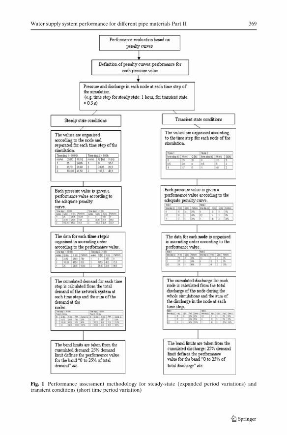
In a similar way as mentioned in Tamminen et al. (2008), the performance indexvaries between a no-service (0%) and an optimum-service (100%) situation, andthe curves are supposed to penalise any deviation from the latter. The conventionadopted means: 100% for optimum service, 75% for adequate service, 50% foracceptable service, 25% for unacceptable service and 0% for no service. Hence, thismethod yields values of performance evaluation for every element of a network, aswell as for the network as a whole. Based on several simulations for an extendedperiod of a day to analyse the quasi-stable operation and for small instants toanalyse the transient regimes during the normal system operation, the behaviour isachieved through a function to represent the performance assessment, which lendsto a basic statistical treatment. The two situations are combined together graphicallyin diagrams, where performance is plotted against simulation period, typically a 24-hsimulation for steady state conditions and against different pipe sections for unsteadyconditions, since the pressure variations are rapid phenomena with the notoriouspressure peaks, in general, close to the manoeuvre device (e.g., a valve or a pump;Fig. 1).

This analysis allows one to detect critical pipe sections and eventual resonanceeffects induced by the dynamic system behaviour and pressure waves overlapping.

Water supply system performance for different pipe materials Part II 369

Fig. 1 Performance assessment methodology for steady-state (expanded period variations) andtransient conditions (short time period variation)

370 H. Ramos et al.

2 Fundamentals

2.1 Flow Models

In order to guarantee an adequate technique performance of a water system, it isnecessary to be able to globally evaluate the system behaviour, which includes dif-ferent scenarios by means of operational conditions for different restrictions of eachcomponent. The hydraulic simulation of the systems is developed by using routinesbased on EPANET 2.0 (Rossman 2000) for steady conditions and on WANDA(WL/Delft) for transient conditions. For the performance evaluation specific modelswere developed based on penalty curves adequately formulated to analyse the systembehaviour for each flow condition based on the typical system actions enabling thusa best understanding of each physical phenomena.

Extended period simulations normally involve several simulations for differentoperating conditions. This is a sequence of steady state simulations for whichboundary conditions are updated in order to reflect changes in nodal demands,tank levels, pump operation, valve regulation, leakage occurrence (Giustolisi andDoglioni 2007). In order to reproduce the behaviour of water distribution networks,hydraulic models for steady-state analyses have been presented in the literature.They normally seek for extended period modelling process through the developmentof hydraulic solvers based on pressure-dependent demands (Araujo et al. 2003, 2006;Fujiwara and Li 1998; Martínez et al. 1999; Soares et al. 2003; Tanyimboh et al. 2001;Todini 2003; Tucciarelli et al. 1999). Regarding to unsteady flow conditions, severalresearchers have developed different analysis based on the occurrence dynamiceffects in water pipe systems when induced by hydromechanical devices manoeuvres(Ramos 1995; Brunone and Morelli 1999; McInnis and Karney 1995; Loureiro et al.2002; Stephens et al. 2005; Covas et al. 2004, 2005) sometimes based on field tests,on computer simulations and optimization procedures and dynamic pipe wall be-haviour. Other researchers (Fleming et al. 2006; Gullick et al. 2004; Karim et al.2003) analysed the effect of occurrence of transient low and negative pressures indistribution systems.

Unsteady analysis usually focuses on the estimation of the extreme pressures asso-ciated with the worse case scenarios. Valve manoeuvres, pump trip-off and start-up,accidental pipe bursts, flood occurrence with soil slices or seismic actions are typicalevents that generate fluid transients that are rarely considered in pipe system design.However the type of actions which induce stronger effects on the pressure variationare well known, but the correct prediction of the pressure wave propagation, inparticular the overlapping of wave propagation effects in different pipe branches andthe occurrence of unconventional dynamic effects are not always properly accountedfor, which will influence the system re-operation. These dynamic conditions induceincreased difficulties in the model calibration and diagnosis analysis for fore sightingthe system response.

Considering the flow mainly one-dimensional (1D) due to the system being longerthan thicker, hydraulic transients in pressurised pipe systems can be satisfactorily de-scribed by a linear elastic model, according to the following assumptions (Chaudhry1987; Almeida and Koelle 1992; Wylie and Streeter 1993): (1) the flow is consideredwith a pseudo-uniform velocity profile in each cross-section; (2) the fluid is assumedone-phase, homogeneous, compressible and with negligible temperature and density


changes; (3) the rheological behaviour of the pipe material is linear-elastic; (4) thepipe is a straight uniform element without lateral inflow or outflow (5) the pipe iscompletely constrained from movement.

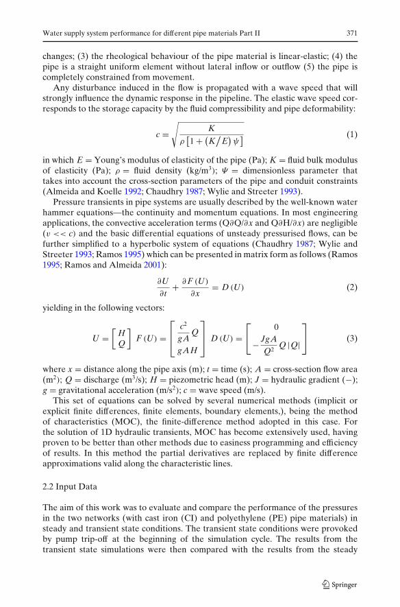
Any disturbance induced in the flow is propagated with a wave speed that willstrongly influence the dynamic response in the pipeline. The elastic wave speed cor-responds to the storage capacity by the fluid compressibility and pipe deformability:

c =√

K

ρ[1 + (

K/

E)ψ

] (1)

in which E = Young’s modulus of elasticity of the pipe (Pa); K = fluid bulk modulusof elasticity (Pa); ρ = fluid density (kg/m3); Ψ = dimensionless parameter thattakes into account the cross-section parameters of the pipe and conduit constraints(Almeida and Koelle 1992; Chaudhry 1987; Wylie and Streeter 1993).

Pressure transients in pipe systems are usually described by the well-known waterhammer equations—the continuity and momentum equations. In most engineeringapplications, the convective acceleration terms (Q∂Q/∂x and Q∂H/∂x) are negligible(v << c) and the basic differential equations of unsteady pressurised flows, can befurther simplified to a hyperbolic system of equations (Chaudhry 1987; Wylie andStreeter 1993; Ramos 1995) which can be presented in matrix form as follows (Ramos1995; Ramos and Almeida 2001):

∂U∂t

+ ∂ F (U)

∂x= D (U) (2)

yielding in the following vectors:

U =[

HQ

]F (U) =

⎡⎢⎣

c2

gAQ

gAH

⎤⎥⎦ D (U) =

⎡⎣ 0

− JgAQ2

Q |Q|

⎤⎦ (3)

where x = distance along the pipe axis (m); t = time (s); A = cross-section flow area(m2); Q = discharge (m3/s); H = piezometric head (m); J = hydraulic gradient (−);g = gravitational acceleration (m/s2); c = wave speed (m/s).

This set of equations can be solved by several numerical methods (implicit orexplicit finite differences, finite elements, boundary elements,), being the methodof characteristics (MOC), the finite-difference method adopted in this case. Forthe solution of 1D hydraulic transients, MOC has become extensively used, havingproven to be better than other methods due to easiness programming and efficiencyof results. In this method the partial derivatives are replaced by finite differenceapproximations valid along the characteristic lines.

2.2 Input Data

The aim of this work was to evaluate and compare the performance of the pressuresin the two networks (with cast iron (CI) and polyethylene (PE) pipe materials) insteady and transient state conditions. The transient state conditions were provokedby pump trip-off at the beginning of the simulation cycle. The results from thetransient state simulations were then compared with the results from the steady

372 H. Ramos et al.

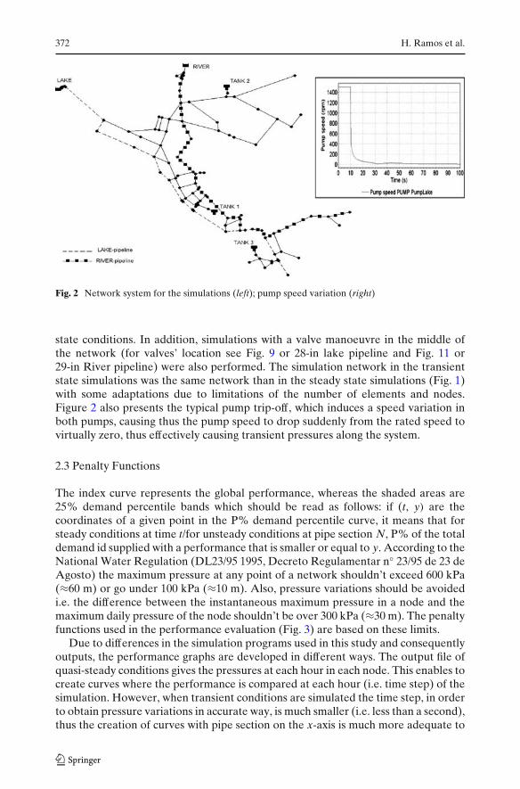
Fig. 2 Network system for the simulations (left); pump speed variation (right)

state conditions. In addition, simulations with a valve manoeuvre in the middle ofthe network (for valves’ location see Fig. 9 or 28-in lake pipeline and Fig. 11 or29-in River pipeline) were also performed. The simulation network in the transientstate simulations was the same network than in the steady state simulations (Fig. 1)with some adaptations due to limitations of the number of elements and nodes.Figure 2 also presents the typical pump trip-off, which induces a speed variation inboth pumps, causing thus the pump speed to drop suddenly from the rated speed tovirtually zero, thus effectively causing transient pressures along the system.

2.3 Penalty Functions

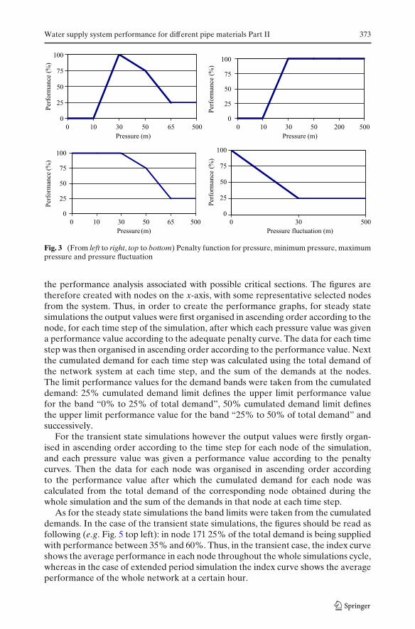
The index curve represents the global performance, whereas the shaded areas are25% demand percentile bands which should be read as follows: if (t, y) are thecoordinates of a given point in the P% demand percentile curve, it means that forsteady conditions at time t/for unsteady conditions at pipe section N, P% of the totaldemand id supplied with a performance that is smaller or equal to y. According to theNational Water Regulation (DL23/95 1995, Decreto Regulamentar n◦ 23/95 de 23 deAgosto) the maximum pressure at any point of a network shouldn’t exceed 600 kPa(≈60 m) or go under 100 kPa (≈10 m). Also, pressure variations should be avoidedi.e. the difference between the instantaneous maximum pressure in a node and themaximum daily pressure of the node shouldn’t be over 300 kPa (≈30 m). The penaltyfunctions used in the performance evaluation (Fig. 3) are based on these limits.

Due to differences in the simulation programs used in this study and consequentlyoutputs, the performance graphs are developed in different ways. The output file ofquasi-steady conditions gives the pressures at each hour in each node. This enables tocreate curves where the performance is compared at each hour (i.e. time step) of thesimulation. However, when transient conditions are simulated the time step, in orderto obtain pressure variations in accurate way, is much smaller (i.e. less than a second),thus the creation of curves with pipe section on the x-axis is much more adequate to


0 30 500

Pressure fluctuation (m)

Per

form

ance

(%

)0

25

50

75

100

0

25

50

75

100

0

25

50

75

100

0

25

50

75

100

0 10 30 50 65 500

0 10 30 50 65 500

Pressure (m)

Per

form

ance

(%

)

0 10 30 50 200 500

Pressure (m)

Per

form

ance

(%

)

Pressure (m)

Per

form

ance

(%

)

Fig. 3 (From left to right, top to bottom) Penalty function for pressure, minimum pressure, maximumpressure and pressure fluctuation

the performance analysis associated with possible critical sections. The figures aretherefore created with nodes on the x-axis, with some representative selected nodesfrom the system. Thus, in order to create the performance graphs, for steady statesimulations the output values were first organised in ascending order according to thenode, for each time step of the simulation, after which each pressure value was givena performance value according to the adequate penalty curve. The data for each timestep was then organised in ascending order according to the performance value. Nextthe cumulated demand for each time step was calculated using the total demand ofthe network system at each time step, and the sum of the demands at the nodes.The limit performance values for the demand bands were taken from the cumulateddemand: 25% cumulated demand limit defines the upper limit performance valuefor the band “0% to 25% of total demand”, 50% cumulated demand limit definesthe upper limit performance value for the band “25% to 50% of total demand” andsuccessively.

For the transient state simulations however the output values were firstly organ-ised in ascending order according to the time step for each node of the simulation,and each pressure value was given a performance value according to the penaltycurves. Then the data for each node was organised in ascending order accordingto the performance value after which the cumulated demand for each node wascalculated from the total demand of the corresponding node obtained during thewhole simulation and the sum of the demands in that node at each time step.

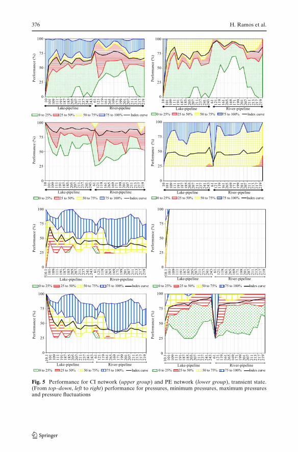
As for the steady state simulations the band limits were taken from the cumulateddemands. In the case of the transient state simulations, the figures should be read asfollowing (e.g. Fig. 5 top left): in node 171 25% of the total demand is being suppliedwith performance between 35% and 60%. Thus, in the transient case, the index curveshows the average performance in each node throughout the whole simulations cycle,whereas in the case of extended period simulation the index curve shows the averageperformance of the whole network at a certain hour.

374 H. Ramos et al.

In the analysed system can be distinguished two water trunk-main pipelines (i.e.the lake-pipeline and the river-pipeline), the pipeline downstream from the lake-reservoir and the pipeline downstream from the river reservoir (Fig. 2). These twopipeline systems even connect themselves are used in the present analyses in orderto facilitate the better interpretation of the dynamic behaviour and the systeminteraction as a whole.

3 Pressure Performance Analysis

3.1 Introduction

Recent developments based on the flow acceleration/deceleration, mechanical re-sponses of the pipe-wall material and leakage influence are analysed in order tobetter understand the pipe system response under steady and transient conditionsfor pressurised flows. Pressure variations, which naturally occur in pipe systems,propagate back and forth along the pipes. Water hammer analysis is very importantin the design of water pipeline systems to select pipe materials, to size wall thickness,in order to sustain pressure ratings and to specify surge protection devices, as wellas during the system exploitation for different operating conditions. This researchpresents the main dynamic effects associated to normal operation that usually occurin water pipe systems but analysed under the point of view of system performanceevaluation.

A well-known problem consists in the inability to predict the fluid pressure varia-tion due to the discharge (or demand) variation or manoeuvres in hydromechanicalequipments induced by pumps and valves, and the associated system performed. Inaddition, there is a lack of knowledge for new pipe materials (i.e. PE pipes) to supporta physical understanding of how the system behaviour influences the pressurevariation and its performance along the pipe system. Even though the knowledge ofthe type of actions that induce stronger effects on the pressure variation is significant,the correct prediction of system response, is not always properly accounted for, whichwill influence the system vulnerability index.

3.2 Performance Evaluation

3.2.1 Pump Trip-off

In the first simulation transient pressures in the system were provoked by stop-ping both pumps—the pump downstream from the river-reservoir and the pumpdownstream from the lake-reservoir—at the first period (few seconds to obtain theextreme pressure peaks) of the simulation cycle.

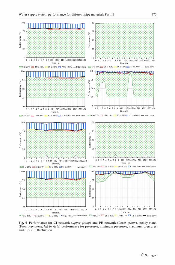
The performance simulation diagram for steady state pressures (Fig. 4) shows thatthe average performance of the system is in the region of 80% and 25% of the totaldemand is being supplied with higher than 80% performance. The 25% demand bandstretches to 0% performances due to a few nodes with low performances—namelythe nodes immediately downstream from the tanks. The performance simulationdiagram for the transient pressures (Fig. 5) shows an average performance between50% and 75%. In the beginning of the lake-pipeline, node 10 has low performancesdue to very low pressures occurring in this node. It should be noted thus that this


0

25

50

75

100

0 1 2 3 4 5 6 7 8 9 101112131415161718192021222324

Time (h)

)%(

ec

na

mrofr

eP

0 to 25% 25 to 50% 50 to 75% 75 to 100% Index curve

0

25

50

75

100

0 1 2 3 4 5 6 7 8 9 101112131415161718192021222324

Time (h)

)%(

ec

na

mrof r

eP


0

25

50

75

100

0 1 2 3 4 5 6 7 8 9 101112131415161718192021222324

Time (h)

)%(

ec

na

mrof r

eP


0

25

50

75

100

0 1 2 3 4 5 6 7 8 9 101112131415161718192021222324

Time (h)

)%(

ec

na

mrofr

eP


0

25

50

75

100

0 1 2 3 4 5 6 7 8 9 101112131415161718192021222324

Time (h)

)%(

ec

na

mrofr

eP


0

25

50

75

100

0 1 2 3 4 5 6 7 8 9 101112131415161718192021222324

Time (h)

)%(

ec

na

m ro fr

eP

0 to 25% 25 to 50% 50 to 75% 75 to 100%

0

25

50

75

100

0 1 2 3 4 5 6 7 8 9 101112131415161718192021222324

Time (h)

)%(

ec

na

mrofr

eP


0

25

50

75

100

0 1 2 3 4 5 6 7 8 9 101112131415161718192021222324

Time (h)

)%(

ec

na

mrof r

eP


Fig. 4 Performance for CI network (upper group) and PE network (lower group), steady state.(From top–down, left to right) performance for pressures, minimum pressures, maximum pressuresand pressure fluctuation

376 H. Ramos et al.

0

25

50

75

100

10

10

11

09

11

11

91

18

71

85

20

52

07

21

12

37

24

12

43

61

12

11

19

16

12

65

16

91

71

19

92

01

20

72

11

21

32

17

21

9

Per

form

ance

(%

)


River-pipelineLake-pipeline

0

25

50

75

100

10

10

11

09

11

11

91

18

71

85

20

52

07

21

12

37

24

12

43

61

12

11

19

16

12

65

16

91

71

19

92

01

20

72

11

21

32

17

21

9

Perf

orm

an

ce (

%)



0

25

50

75

100

10

10

11

09

11

11

91

18

71

85

20

52

07

21

12

37

24

12

43

61

12

11

19

16

12

65

16

91

71

19

92

01

20

72

11

21

32

17

21

9

Per

form

ance

(%

)



0

25

50

75

100

10

10

11

09

11

11

91

18

71

85

20

52

07

21

12

37

24

12

43

61

12

11

19

16

12

65

16

91

71

19

92

01

20

72

11

21

32

17

21

9

Perf

orm

an

ce (

%)


Lake-pipeline River-pipeline

0

25

50

75

100

10

.11

01

10

91

11

19

11

87

18

52

05

20

72

11

23

72

41

24

36

11

21

11

91

61

26

51

69

17

11

99

20

12

07

21

12

13

21

72

19

Perf

orm

an

ce (

%)



0

25

50

75

100

10

.11

01

10

91

11

19

11

87

18

52

05

20

72

11

23

72

41

24

36

11

21

11

91

61

26

51

69

17

11

99

20

12

07

21

12

13

21

72

19

Perf

orm

an

ce (

%)



10

.11

01

10

91

11

19

11

87

18

52

05

20

72

11

23

72

41

24

36

11

21

11

91

61

26

51

69

17

11

99

20

12

07

21

12

13

21

72

19

Perf

orm

an

ce (

%)



0

25

50

75

100

0

25

50

75

100

10

.11

01

10

91

11

19

11

87

18

52

05

20

72

11

23

72

41

24

36

11

21

11

91

61

26

51

69

17

11

99

20

12

07

21

12

13

21

72

19

Perf

orm

an

ce (

%)



Fig. 5 Performance for CI network (upper group) and PE network (lower group), transient state.(From top–down, left to right) performance for pressures, minimum pressures, maximum pressuresand pressure fluctuations


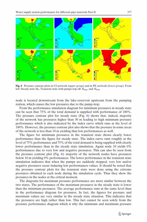
Fig. 6 Pressure contour plots in CI network (upper group) and in PE network (lower group). Fromleft: Steady state H0, Transient state with pumps trip-off Hmin, and Hmax

node is located downstream from the lake-reservoir upstream from the pumpingstation, which causes the low pressures due to the pump stop.

From the performance simulation diagram for minimum pressures in steady statecan be seen that 75% of the total demand is supplied with performance of 100%.The pressure contour plot for steady state (Fig. 6) shows that, indeed, majorityof the network has pressures higher than 30 m leading to high minimum pressureperformance which is also indicated by the index curve which runs at the level of100%. However, the pressure contour plot also shows that the pressure in some areasof the network is less than 10 m yielding thus low performances as well.

The figure for minimum pressures in the transient state shows clearly lowerperformance than the figure for steady state. The index curve runs roughly at thelevel of 75% performance and 75% of the total demand is being supplied with clearlylower performance than in the steady state simulation. Again node 10 yields 0%performances due to very low and negative pressures. This can also be seen fromthe pressure contour plot (Fig. 6): majority of the network nodes have pressuresbelow 10 m yielding 0% performances. The lower performance in the transient statesimulation indicates that when the pumps are suddenly stopped, very low and/ornegative pressures occur inducing low performances values. It should be noted thatthe pressure contour plots for the transient state were done using the extremepressures obtained in each node during the simulation cycle. Thus they show thepressures in the nodes at the critical moment.

The diagrams for maximum pressure performance are more similar between thetwo states. The performance of the maximum pressures in the steady state is lowerthan the minimum pressures. The average performance runs at the same level thanin the performance diagram for pressures. In fact, the figures for pressure andmaximum values are very similar in the steady state situation. This indicates thatthe pressures are high rather than low. This fact cannot be seen solely from thepressure performance diagram which is why the minimum and maximum pressure

378 H. Ramos et al.

performance diagrams are made to allow more detailed analysis of the pressures inthe system. In the case of transient state, however, the maximum pressure diagramis different from the pressure diagram. The average performance is slightly higher inthe maximum pressure diagram and the performances never reach very low values; inmost part of the pipelines the performance maintains above 50% limit. In addition,the performance of the maximum pressures is better than the performance of theminimum pressures. This suggests that in transient state the pressures are rather lowthan high—even though the average performance is quite high in both diagrams—contrary to the situation in steady state. Thus, as mentioned earlier, the suddenstopping of the pumps creates low and/or negative pressures.

From the pressure fluctuation figure can be seen that the pressure does not varymuch in the steady state simulations. The average performance is high and 75% ofthe total demand is supplied with performance higher than 90%. This is expectablesince there are no incidents provoking high or low pressures in the steady state. Inthe transient state, however, the situation is quite different. Even though it is notpossible to tell whether the system has dominantly high or low pressures from thepressure variation, minimum pressure and maximum pressure diagrams, since theyhave all fairly high performances, however the pressure fluctuation diagram indicatesthat there are big variations in the pressure of the system. The diagram shows thatthe performance is fairly low. This is probably due to the pressure peaks that occurin the nodes in the beginning of the simulation cycle when the pumps are suddenlystopped.

The simulations in the PE network were done similarly with the CI network.Some changes in the input data were necessary to adjust the pipe characteristics (i.e.pipe roughness, pipe-wall thickness, Young’s modulus of elasticity of the pipe, wavespeed).

The steady state pressure performance diagram (Fig. 4) indicates that the perfor-mance is fairly good. The index curve runs at a level over 75%. From the contourplot for the steady state it can be seen that the pressures are mainly over 30 myielding good performances. The pressure diagram for transient state (Fig. 5) haslower performance.

Regarding the minimum pressures the figures for steady state and transient stateare fairly similar. The 0% performances in the steady state are caused by a fewnodes in the system mainly downstream from the tanks. However, the index curvesdemonstrate that in both conditions the system’s performance is in the range ofoptimum service. This can also be seen from the contour plots (Fig. 6): the pressuresin both conditions are mainly over 30 m, which returns performances of 100%.

The figures for maximum pressures are, however, fairly different. The index curveruns in majority of the pipelines below 50% performance limit. In the steady statesituation the performances are better and the index curve also runs roughly at the75% performance limit. In addition, the contour plots show that in the steady statethe pressures are mainly between 30 and 50 m which return performances between75% and 100%. However, in transient state big part of the network have pressuresabove 65 m which return performances of only 25%.

The minimum pressure performances are clearly higher in the PE network, whichindicates that the pressures are higher in the PE network than in the CI network.

However, the performance of the pressure fluctuation in the PE network is clearlybetter than in the CI network, which suggests that the pressure peaks in the PE


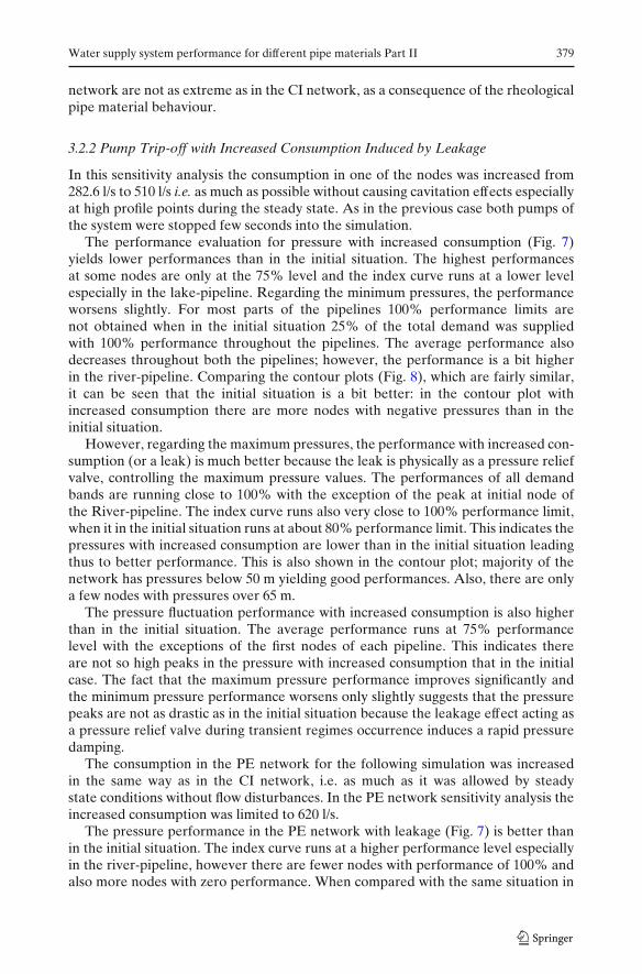
network are not as extreme as in the CI network, as a consequence of the rheologicalpipe material behaviour.

3.2.2 Pump Trip-off with Increased Consumption Induced by Leakage

In this sensitivity analysis the consumption in one of the nodes was increased from282.6 l/s to 510 l/s i.e. as much as possible without causing cavitation effects especiallyat high profile points during the steady state. As in the previous case both pumps ofthe system were stopped few seconds into the simulation.

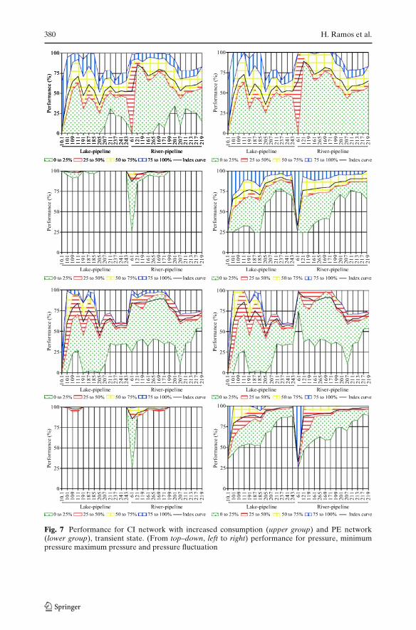
The performance evaluation for pressure with increased consumption (Fig. 7)yields lower performances than in the initial situation. The highest performancesat some nodes are only at the 75% level and the index curve runs at a lower levelespecially in the lake-pipeline. Regarding the minimum pressures, the performanceworsens slightly. For most parts of the pipelines 100% performance limits arenot obtained when in the initial situation 25% of the total demand was suppliedwith 100% performance throughout the pipelines. The average performance alsodecreases throughout both the pipelines; however, the performance is a bit higherin the river-pipeline. Comparing the contour plots (Fig. 8), which are fairly similar,it can be seen that the initial situation is a bit better: in the contour plot withincreased consumption there are more nodes with negative pressures than in theinitial situation.

However, regarding the maximum pressures, the performance with increased con-sumption (or a leak) is much better because the leak is physically as a pressure reliefvalve, controlling the maximum pressure values. The performances of all demandbands are running close to 100% with the exception of the peak at initial node ofthe River-pipeline. The index curve runs also very close to 100% performance limit,when it in the initial situation runs at about 80% performance limit. This indicates thepressures with increased consumption are lower than in the initial situation leadingthus to better performance. This is also shown in the contour plot; majority of thenetwork has pressures below 50 m yielding good performances. Also, there are onlya few nodes with pressures over 65 m.

The pressure fluctuation performance with increased consumption is also higherthan in the initial situation. The average performance runs at 75% performancelevel with the exceptions of the first nodes of each pipeline. This indicates thereare not so high peaks in the pressure with increased consumption that in the initialcase. The fact that the maximum pressure performance improves significantly andthe minimum pressure performance worsens only slightly suggests that the pressurepeaks are not as drastic as in the initial situation because the leakage effect acting asa pressure relief valve during transient regimes occurrence induces a rapid pressuredamping.

The consumption in the PE network for the following simulation was increasedin the same way as in the CI network, i.e. as much as it was allowed by steadystate conditions without flow disturbances. In the PE network sensitivity analysis theincreased consumption was limited to 620 l/s.

The pressure performance in the PE network with leakage (Fig. 7) is better thanin the initial situation. The index curve runs at a higher performance level especiallyin the river-pipeline, however there are fewer nodes with performance of 100% andalso more nodes with zero performance. When compared with the same situation in

380 H. Ramos et al.

Fig. 7 Performance for CI network with increased consumption (upper group) and PE network(lower group), transient state. (From top–down, left to right) performance for pressure, minimumpressure maximum pressure and pressure fluctuation


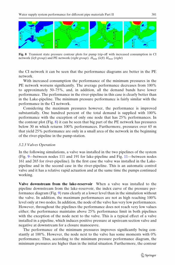
Fig. 8 Transient state pressure contour plots for pump trip-off with increased consumption in CInetwork (left group) and PE network (right group). Hmin (left) Hmax (right)

the CI network it can be seen that the performance diagrams are better in the PEnetwork.

With increased consumption the performance of the minimum pressures in thePE network worsens significantly. The average performance decreases from 100%to approximately 50–75%, and, in addition, all the demand bands have lowerperformance. The performance in the river-pipeline in this case is clearly better thanin the Lake-pipeline. The minimum pressure performance is fairly similar with theperformance in the CI network.

Considering the maximum pressures however, the performance is improvedsubstantially. One hundred percent of the total demand is supplied with 100%performance with the exception of only one node that has 25% performances. Inthe contour plot (Fig. 8) it can be seen that big part of the PE network has pressuresbelow 30 m which returns 100% performances. Furthermore, pressures over 65 mthat yield 25% performance are only in a small area of the network in the beginningof the river-pipeline in the pump-station.

3.2.3 Valves Operation

In the following simulations, a valve was installed in the two pipelines of the system(Fig. 9—between nodes 111 and 191 for lake-pipeline and Fig. 11—between nodes161 and 265 for river-pipeline). In the first case the valve was installed in the Lake-pipeline and in the second case in the river-pipeline. This is an automatic controlvalve and it has a relative rapid actuation and at the same time the pumps continuedworking.

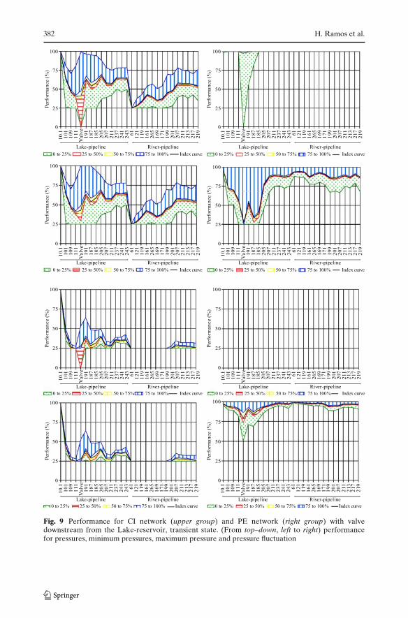
Valve downstream from the lake-reservoir When a valve was installed to thepipeline downstream from the lake-reservoir, the index curve of the pressure per-formance diagram (Fig. 9) runs clearly at a lower level than in the simulation withoutthe valve. In addition, the maximum performances are not as high reaching 100%level only at two nodes. In addition, the node of the valve has very low performances.However, throughout the pipelines the performance does not reach very low valueseither; the performance maintains above 25% performance limit in both pipelineswith the exception of the node next to the valve. This is a typical effect of a valveinstalled in a pipeline, which induces positive pressure at upstream section valve andnegative at downstream for a closure manoeuvre.

The performance of the minimum pressures improves significantly being con-stantly at 100%. However, the node next to the valve has some moments with 0%performance. Thus, according to the minimum pressure performance diagram, theminimum pressures are higher than in the initial situation. Furthermore, the contour

382 H. Ramos et al.

Fig. 9 Performance for CI network (upper group) and PE network (right group) with valvedownstream from the Lake-reservoir, transient state. (From top–down, left to right) performancefor pressures, minimum pressures, maximum pressure and pressure fluctuation


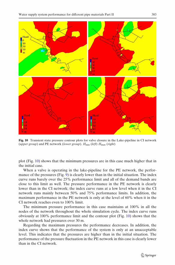
Fig. 10 Transient state pressure contour plots for valve closure in the Lake-pipeline in CI network(upper group) and PE network (lower group). Hmin (left) Hmax (right)

plot (Fig. 10) shows that the minimum pressures are in this case much higher that inthe initial case.

When a valve is operating in the lake-pipeline for the PE network, the perfor-mance of the pressures (Fig. 9) is clearly lower than in the initial situation. The indexcurve runs barely over the 25% performance limit and all of the demand bands areclose to this limit as well. The pressure performance in the PE network is clearlylower than in the CI network; the index curve runs at a low level when it in the CInetwork runs mainly between 50% and 75% performance limits. In addition, themaximum performance in the PE network is only at the level of 60% when it in theCI network reaches even to 100% limit.

The minimum pressure performance in this case maintains at 100% in all thenodes of the network throughout the whole simulation cycle. The index curve runsobviously at 100% performance limit and the contour plot (Fig. 10) shows that thewhole network had pressures over 30 m.

Regarding the maximum pressures the performance decreases. In addition, theindex curve shows that the performance of the system is only at an unacceptablelevel. This indicates that the pressures are higher than in the initial situation. Theperformance of the pressure fluctuation in the PE network in this case is clearly lowerthan in the CI network.

384 H. Ramos et al.

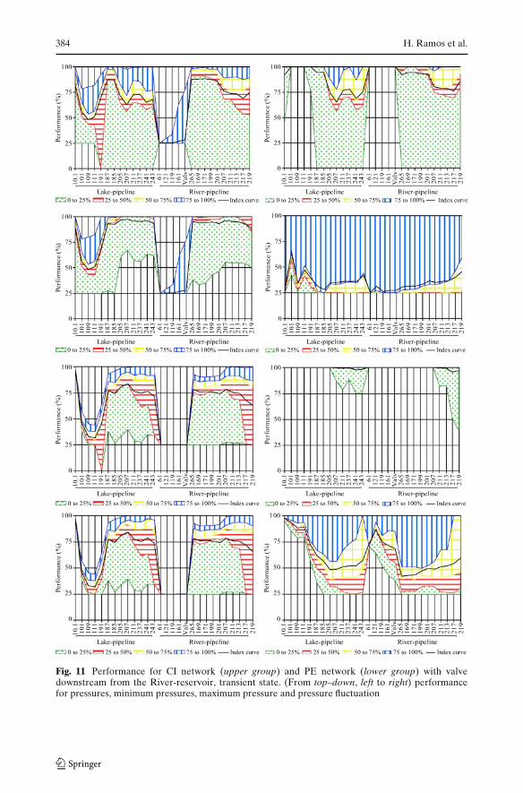
Fig. 11 Performance for CI network (upper group) and PE network (lower group) with valvedownstream from the River-reservoir, transient state. (From top–down, left to right) performancefor pressures, minimum pressures, maximum pressure and pressure fluctuation


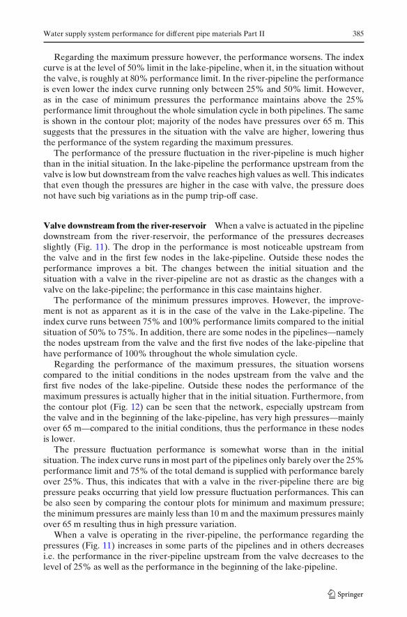
Regarding the maximum pressure however, the performance worsens. The indexcurve is at the level of 50% limit in the lake-pipeline, when it, in the situation withoutthe valve, is roughly at 80% performance limit. In the river-pipeline the performanceis even lower the index curve running only between 25% and 50% limit. However,as in the case of minimum pressures the performance maintains above the 25%performance limit throughout the whole simulation cycle in both pipelines. The sameis shown in the contour plot; majority of the nodes have pressures over 65 m. Thissuggests that the pressures in the situation with the valve are higher, lowering thusthe performance of the system regarding the maximum pressures.

The performance of the pressure fluctuation in the river-pipeline is much higherthan in the initial situation. In the lake-pipeline the performance upstream from thevalve is low but downstream from the valve reaches high values as well. This indicatesthat even though the pressures are higher in the case with valve, the pressure doesnot have such big variations as in the pump trip-off case.

Valve downstream from the river-reservoir When a valve is actuated in the pipelinedownstream from the river-reservoir, the performance of the pressures decreasesslightly (Fig. 11). The drop in the performance is most noticeable upstream fromthe valve and in the first few nodes in the lake-pipeline. Outside these nodes theperformance improves a bit. The changes between the initial situation and thesituation with a valve in the river-pipeline are not as drastic as the changes with avalve on the lake-pipeline; the performance in this case maintains higher.

The performance of the minimum pressures improves. However, the improve-ment is not as apparent as it is in the case of the valve in the Lake-pipeline. Theindex curve runs between 75% and 100% performance limits compared to the initialsituation of 50% to 75%. In addition, there are some nodes in the pipelines—namelythe nodes upstream from the valve and the first five nodes of the lake-pipeline thathave performance of 100% throughout the whole simulation cycle.

Regarding the performance of the maximum pressures, the situation worsenscompared to the initial conditions in the nodes upstream from the valve and thefirst five nodes of the lake-pipeline. Outside these nodes the performance of themaximum pressures is actually higher that in the initial situation. Furthermore, fromthe contour plot (Fig. 12) can be seen that the network, especially upstream fromthe valve and in the beginning of the lake-pipeline, has very high pressures—mainlyover 65 m—compared to the initial conditions, thus the performance in these nodesis lower.

The pressure fluctuation performance is somewhat worse than in the initialsituation. The index curve runs in most part of the pipelines only barely over the 25%performance limit and 75% of the total demand is supplied with performance barelyover 25%. Thus, this indicates that with a valve in the river-pipeline there are bigpressure peaks occurring that yield low pressure fluctuation performances. This canbe also seen by comparing the contour plots for minimum and maximum pressure;the minimum pressures are mainly less than 10 m and the maximum pressures mainlyover 65 m resulting thus in high pressure variation.

When a valve is operating in the river-pipeline, the performance regarding thepressures (Fig. 11) increases in some parts of the pipelines and in others decreasesi.e. the performance in the river-pipeline upstream from the valve decreases to thelevel of 25% as well as the performance in the beginning of the lake-pipeline.

386 H. Ramos et al.

Fig. 12 Transient state pressure contour plots for valve closure in the River-pipeline in CI network(upper group) and PE network (lower group). Hmin (left) Hmax (right)

Regarding the minimum pressures the situation stays more or less the samecompared to the initial situation. Majority of the nodes have performance of 100%and only few nodes have performance lower than this, which can be seen fromthe contour plot as well (Fig. 12). In the contour plot majority of the network haspressures above 30 m yielding thus 100% performance. The performance of theminimum pressures in the PE network is thus much better than that in the CInetwork. In the CI network there are nodes with zero performance and the indexcurve runs at points at a much lower level than in the PE network.

Regarding the maximum pressures, the situation is very similar to that regard-ing the performance of the total pressures. When compared with the situationof the valve in the lake-pipeline, the performances tend to be much higher. Theperformance in the CI network in this same situation is fairly similar with theperformance in PE network.

The pressure fluctuation performances with a valve operating in the river-pipelineare lower than in the initial situation. This indicates that there are more extremepressure peaks in the system. Compared with the performance in the CI network theperformances in the PE network are exactly the opposite: in the nodes where theperformance is high in the CI network it is lower in the PE network and vice versa.


4 Pressure Variation in the Pipelines

4.1 Pump Trip-off

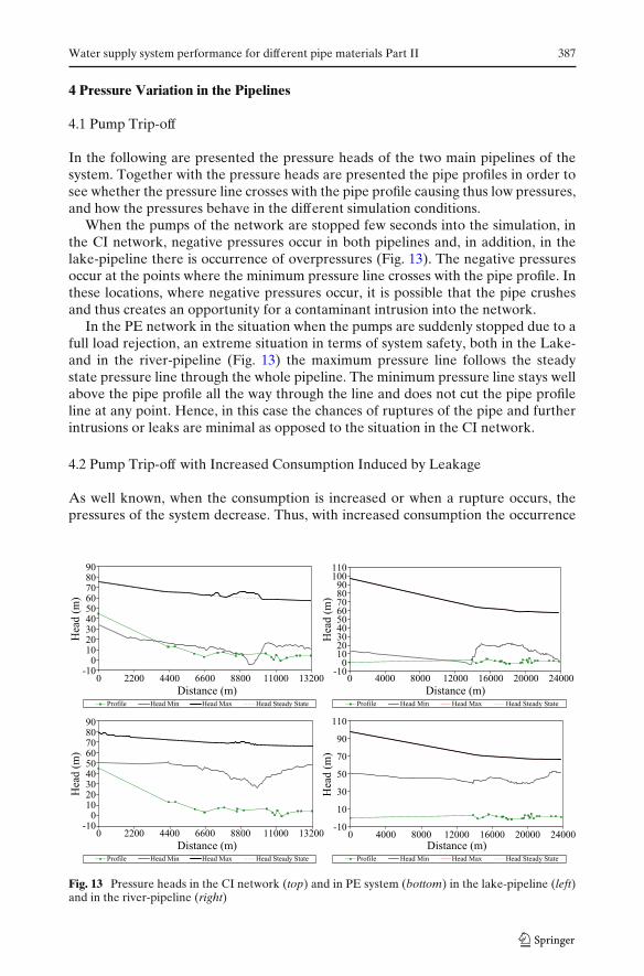
In the following are presented the pressure heads of the two main pipelines of thesystem. Together with the pressure heads are presented the pipe profiles in order tosee whether the pressure line crosses with the pipe profile causing thus low pressures,and how the pressures behave in the different simulation conditions.

When the pumps of the network are stopped few seconds into the simulation, inthe CI network, negative pressures occur in both pipelines and, in addition, in thelake-pipeline there is occurrence of overpressures (Fig. 13). The negative pressuresoccur at the points where the minimum pressure line crosses with the pipe profile. Inthese locations, where negative pressures occur, it is possible that the pipe crushesand thus creates an opportunity for a contaminant intrusion into the network.

In the PE network in the situation when the pumps are suddenly stopped due to afull load rejection, an extreme situation in terms of system safety, both in the Lake-and in the river-pipeline (Fig. 13) the maximum pressure line follows the steadystate pressure line through the whole pipeline. The minimum pressure line stays wellabove the pipe profile all the way through the line and does not cut the pipe profileline at any point. Hence, in this case the chances of ruptures of the pipe and furtherintrusions or leaks are minimal as opposed to the situation in the CI network.

4.2 Pump Trip-off with Increased Consumption Induced by Leakage

As well known, when the consumption is increased or when a rupture occurs, thepressures of the system decrease. Thus, with increased consumption the occurrence

-100

102030405060708090

0 2200 4400 6600 8800 11000 13200

Distance (m)

Hea

d (

m)

Profile Head Min Head Max Head Steady State

-100

102030405060708090

100110

0 4000 8000 12000 16000 20000 24000

Hea

d (

m)

-100

102030405060708090

0 2200 4400 6600 8800 11000 13200

Distance (m)

Hea

d (

m)




Distance (m)

Distance (m)

-10

10

30

50

70

90

110

0 4000 8000 12000 16000 20000 24000

Hea

d (

m)

Fig. 13 Pressure heads in the CI network (top) and in PE system (bottom) in the lake-pipeline (left)and in the river-pipeline (right)

388 H. Ramos et al.

-10

0

10

20

30

40

50

60

70

80

0 2200 4400 6600 8800 11000 13200

Distance (m)

Hea

d (

m)

-100

102030405060708090

100

0 4000 8000 12000 16000 20000 24000

Hea

d (

m)

-10

0

10

20

30

40

50

60

70

0 2200 4400 6600 8800 11000 13200

Distance (m)

Hea

d (

m)





Distance (m)

Distance (m)

-100

1020304050607080

0 4000 8000 12000 16000 20000 24000

90

Hea

d (

m)

Fig. 14 Pressure heads in the CI network (top) and in PE network (bottom) with increasedconsumption in the lake-pipeline (left) and in the river-pipeline (right)

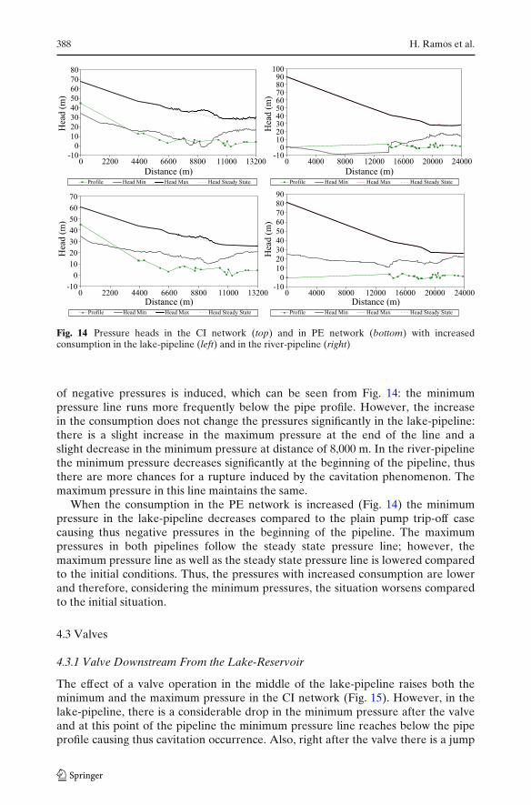
of negative pressures is induced, which can be seen from Fig. 14: the minimumpressure line runs more frequently below the pipe profile. However, the increasein the consumption does not change the pressures significantly in the lake-pipeline:there is a slight increase in the maximum pressure at the end of the line and aslight decrease in the minimum pressure at distance of 8,000 m. In the river-pipelinethe minimum pressure decreases significantly at the beginning of the pipeline, thusthere are more chances for a rupture induced by the cavitation phenomenon. Themaximum pressure in this line maintains the same.

When the consumption in the PE network is increased (Fig. 14) the minimumpressure in the lake-pipeline decreases compared to the plain pump trip-off casecausing thus negative pressures in the beginning of the pipeline. The maximumpressures in both pipelines follow the steady state pressure line; however, themaximum pressure line as well as the steady state pressure line is lowered comparedto the initial conditions. Thus, the pressures with increased consumption are lowerand therefore, considering the minimum pressures, the situation worsens comparedto the initial situation.

4.3 Valves

4.3.1 Valve Downstream From the Lake-Reservoir

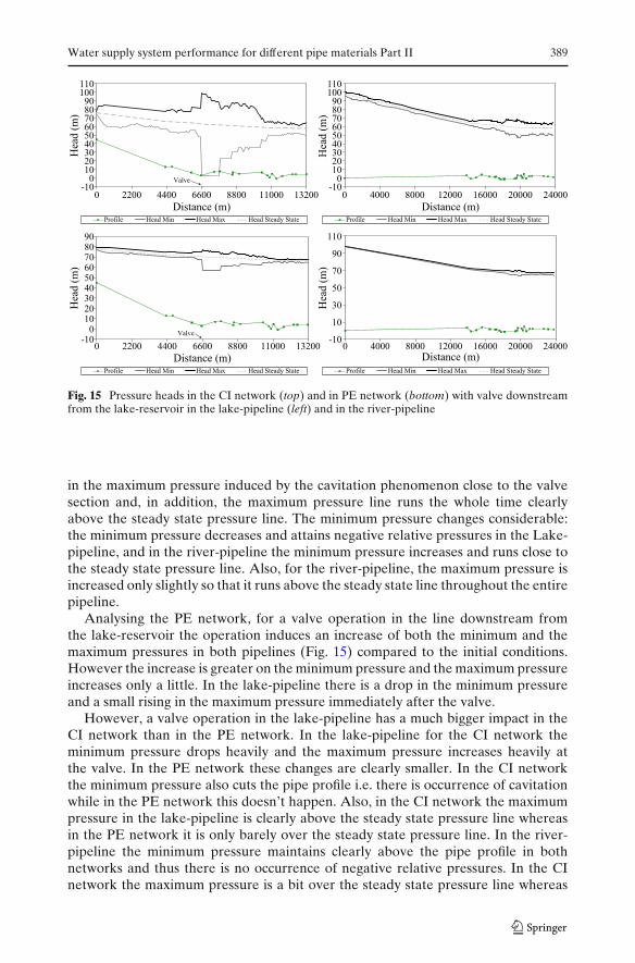
The effect of a valve operation in the middle of the lake-pipeline raises both theminimum and the maximum pressure in the CI network (Fig. 15). However, in thelake-pipeline, there is a considerable drop in the minimum pressure after the valveand at this point of the pipeline the minimum pressure line reaches below the pipeprofile causing thus cavitation occurrence. Also, right after the valve there is a jump


0 2200 4400 6600 8800 11000 13200

Distance (m)

Hea

d (

m)

-100

102030405060708090

100110

0 4000 8000 12000 16000 20000 24000

Hea

d (

m)

-100

102030405060708090

0 2200 4400 6600 8800 11000 13200

Distance (m)

Hea

d (

m)




Distance (m)

Distance (m)

-10

10

30

50

70

90

110

0 4000 8000 12000 16000 20000 24000

Hea

d (

m)


-100

102030405060708090

100110

Valve

Valve

Fig. 15 Pressure heads in the CI network (top) and in PE network (bottom) with valve downstreamfrom the lake-reservoir in the lake-pipeline (left) and in the river-pipeline

in the maximum pressure induced by the cavitation phenomenon close to the valvesection and, in addition, the maximum pressure line runs the whole time clearlyabove the steady state pressure line. The minimum pressure changes considerable:the minimum pressure decreases and attains negative relative pressures in the Lake-pipeline, and in the river-pipeline the minimum pressure increases and runs close tothe steady state pressure line. Also, for the river-pipeline, the maximum pressure isincreased only slightly so that it runs above the steady state line throughout the entirepipeline.

Analysing the PE network, for a valve operation in the line downstream fromthe lake-reservoir the operation induces an increase of both the minimum and themaximum pressures in both pipelines (Fig. 15) compared to the initial conditions.However the increase is greater on the minimum pressure and the maximum pressureincreases only a little. In the lake-pipeline there is a drop in the minimum pressureand a small rising in the maximum pressure immediately after the valve.

However, a valve operation in the lake-pipeline has a much bigger impact in theCI network than in the PE network. In the lake-pipeline for the CI network theminimum pressure drops heavily and the maximum pressure increases heavily atthe valve. In the PE network these changes are clearly smaller. In the CI networkthe minimum pressure also cuts the pipe profile i.e. there is occurrence of cavitationwhile in the PE network this doesn’t happen. Also, in the CI network the maximumpressure in the lake-pipeline is clearly above the steady state pressure line whereasin the PE network it is only barely over the steady state pressure line. In the river-pipeline the minimum pressure maintains clearly above the pipe profile in bothnetworks and thus there is no occurrence of negative relative pressures. In the CInetwork the maximum pressure is a bit over the steady state pressure line whereas

390 H. Ramos et al.

in the PE network both minimum and maximum pressures follow the steady statepressure line.

4.3.2 Valve Downstream From the River-Reservoir

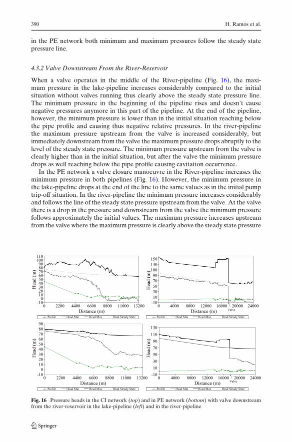
When a valve operates in the middle of the River-pipeline (Fig. 16), the maxi-mum pressure in the lake-pipeline increases considerably compared to the initialsituation without valves running thus clearly above the steady state pressure line.The minimum pressure in the beginning of the pipeline rises and doesn’t causenegative pressures anymore in this part of the pipeline. At the end of the pipeline,however, the minimum pressure is lower than in the initial situation reaching belowthe pipe profile and causing thus negative relative pressures. In the river-pipelinethe maximum pressure upstream from the valve is increased considerably, butimmediately downstream from the valve the maximum pressure drops abruptly to thelevel of the steady state pressure. The minimum pressure upstream from the valve isclearly higher than in the initial situation, but after the valve the minimum pressuredrops as well reaching below the pipe profile causing cavitation occurrence.

In the PE network a valve closure manoeuvre in the River-pipeline increases theminimum pressure in both pipelines (Fig. 16). However, the minimum pressure inthe lake-pipeline drops at the end of the line to the same values as in the initial pumptrip-off situation. In the river-pipeline the minimum pressure increases considerablyand follows the line of the steady state pressure upstream from the valve. At the valvethere is a drop in the pressure and downstream from the valve the minimum pressurefollows approximately the initial values. The maximum pressure increases upstreamfrom the valve where the maximum pressure is clearly above the steady state pressure

0 2200 4400 6600 8800 11000 13200

Distance (m)

Hea

d (

m)

-10

10

30

50

70

90

130

150

0 4000 8000 12000 16000 20000 24000

Hea

d (

m)

-10

0

10

20

30

40

50

60

70

80

90

0 2200 4400 6600 8800 11000 13200

Distance (m)

Hea

d (

m)

Distance (m)

Distance (m)

-10

10

30

50

70

90

110

130

0 4000 8000 12000 16000 20000 24000

Hea

d (

m)





-100

102030405060708090

100110

Valve

Valve

100

Fig. 16 Pressure heads in the CI network (top) and in PE network (bottom) with valve downstreamfrom the river-reservoir in the lake-pipeline (left) and in the river-pipeline


line. At the valve it drops following the steady state pressure line downstream fromthe valve.

Analysing the effect of a valve closure in the river-pipeline it shows—again—stronger effect on the CI network than on the PE network. In the CI network for theRiver-pipeline, the minimum pressure upstream from the valve follows the steadystate pressure line and downstream from the valve decreases below the pipe profilecausing cavitation. The maximum pressure upstream from the valve is clearly abovethe steady state conditions and after the valve it follows the line of the steady stateconditions. In the PE network the pressures also drop downstream from the valve.Upstream from the valve the maximum pressure in the PE network is above thesteady state pressure line and downstream from the valve it follows the steady statepressure line. The minimum pressure behaves the same way as in the CI network butit maintains all the time above the pipe profile. In the Lake-pipeline the maximumpressures in the CI network are much higher than in the PE network. In the PEnetwork the maximum pressure follows the line of the steady state pressure and theminimum pressure does the same in the beginning of the line. In the CI network,however, the maximum pressure is much higher than the steady state pressure lineand also the minimum pressure differs from it much more than in the PE network.In addition, in the CI network the minimum pressure reaches below the pipe profilewhereas in the PE network it maintains above it.

5 Conclusions

The importance of pressure variation analysis including pressure transients is toenable the understanding of how the system behaves in response to a varietyof events such as power outages, pump shut downs, valves’ operation, flushing,firefighting, main breaks and other events that can create significant rapid variationsin system pressure such as sudden high and low pressure waves. Considering pressurevariations, the water companies need to improve the performance index during theoperation of water supply/distribution systems when they are concerned with theimplementation of safety and leakage control policies.

The sensitivity analysis developed for this case study enhances the type of systembehaviour, in especially the performance associated in terms of pressure variationduring normal operations, which allows the following conclusions:

• In the steady state pressure simulations there are no significant differencesbetween the CI and the PE pipe material.

• When the pumps are suddenly trip-off in the PE network the minimum pressuresare evidently higher than in the CI network and the maximum pressures runningroughly at the same level. This is why the minimum pressure performance is verygood in the PE network. The increase in the minimum pressures also means thatthere is clearly less pressure fluctuation than in the CI network meaning that thepressure peaks in the PE network are not as drastic as in the CI network. Thepressure fluctuation performance is therefore better in the PE network than inthe CI network.

• Increasing the consumption in the CI network during a transient event it lowersthe pressures even more yielding thus lower minimum pressure performance andhigher maximum pressure performance. The pressures in the PE network with

392 H. Ramos et al.

increased consumption are noticeably lower than in the plain pump trip-off case,which is why the minimum pressure performance is lower and maximum pressureperformance higher.

• With an operating valve installed in the Lake-pipeline, in the CI network,the minimum pressures in both pipelines get very good minimum pressuresperformance. In the river-pipeline there are no more negative pressures and inthe Lake-pipeline there is negative pressure only immediately downstream thevalve. The pressure fluctuation performance is very good in the river-pipelinesince the maximum and minimum pressures are close to each other. In thePE network downstream from the lake-reservoir the differences between thepressures are small which is why the pressure fluctuation performance is veryhigh, higher than in the pump trip-off case. At the valve there is a small increasein the maximum pressure and a small drop in the minimum pressure, whichcauses the changes in the performance diagrams.

• When an operating valve is located at downstream from the river-reservoir in theCI network, the minimum pressures in the lake-pipeline increase a lot comparedto the plain pump trip-off situation, however compared to the situation withvalve in the lake-pipeline the pressures stay at the same level in the beginning ofthe pipeline. At the end of both pipelines the minimum pressure head goes belowthe pipe profile causing thus negative pressures which yields low performance atthis point of the pipelines. In PE network the maximum pressures in the riverpipeline are high and thus the performance is very low. However at the valvethere is a drop in the pressures and thus the performance increases. Similarbehaviour can be seen in the CI network but with even higher-pressure values.The pressure fluctuation performance is better in PE network than in the CInetwork.

Hence hydraulic and performance models can be used to identify critical be-haviours associated to different pipe materials and hydromechanical manoeuvresin water supply systems, where significant pressure variation and low or negativepressures are most likely to occur. Therefore the analysis developed can be a baseto guide operating managers to the most appropriate monitoring locations, andalso to develop analysis of mitigation techniques for critical situations. Modellingprocesses can in most of times save system operators and money spent on less fruitfulmonitoring efforts or less effective corrective actions.

Acknowledgements The authors wish to thank to FCT through the projects POCTI/ECM/58375/2004 and PTDC/ECM/ 65731/2006 (partly supported by funding under the European Commission—FEDER), as well as CEHIDRO, the Hydro-systems’ research centre from the Department of CivilEngineering, at Instituto Superior Técnico (Lisbon, Portugal).

References

Almeida AB, Koelle E (1992) Fluid transients in pipe networks. Computational Mechanics Publica-tions, Elsevier Applied Science, Amsterdam

Araujo LS, Coelho ST, Ramos HM (2003) Estimation of distributed pressure-dependent leakage andconsumer demand in water supply networks. In: International conference on advances in watersupply management, CCWI 2003, Imperial College, UK

Araujo LS, Ramos H, Coelho ST (2006) Pressure control for leakage minimisation in water distrib-ution systems management. Water Resour Manag 20(1):133–149


Brunone B, Morelli L (1999) Automatic control valve-induced transients in operative pipe system.J Hydraul Eng 125(5):534–542, May

Chaudhry MH (1987) Applied hydraulic transients, 2nd edn. Litton Educational Publishing Inc., VanNostrand Reinhold, New York

Coelho ST (1997) Performance assessment through mathematical modelling. In: Workshop on per-formance indicators for transmission and distribution systems, IWSA, Associação Internacionaldos Distribuidores de Água, National Laboratory of Civil Engineering, Lisbon, Portugal

Covas D, Stoianov I, Mano JF, Ramos H, Graham N, Maksimovic C (2004) The dynamic effect ofpipe-wall viscoelasticity in hydraulic transients. Part I—experimental analysis and creep charac-terization. J Hydraul Res 42(5):516–530

Covas D, Stoianov I, Mano JF, Ramos H, Graham N, Maksimovic C (2005) The dynamic effectof pipe-wall viscoelasticity in hydraulic transients. Part II—model development, calibration andverification. J Hydraul Res 43(1):56–70

Fleming KK, Dugandzic JP, Lechevallier MW, Gullick RW (2006) Susceptibility of potable waterdistribution systems to negative pressure transients. Research project summary. Division ofScience, Research and Technology, Trenton

Fujiwara O, Li J (1998) Reliability analysis of water distribution networks in consideration of equity,redistribution, and pressure-dependent demand. Water Resour Res 34(7):1843–1850, July

Giustolisi O, Doglioni A (2007) A pressure-driven approach for water distribution system modelling.Water Management Challenges in Global Change. Taylor & Francis Group, London, Ulanickiet al. 2007, ISBN 978-0-415-45415-5

Gullick RW, Lechevallier MW, Svinland RC, Friedman MJ (2004) Occurrence of transient low andnegative pressures in distribution systems. J AWWA 96(11):52–66

Karim M, Abbaszadegan M, Lechevallier MW (2003) Potential for pathogen intrusion during pres-sure transients. J AWWA 95(5):134–146

Loureiro D, Ramos H, Coelho ST, Menaia J, Lopes A (2002) Pressure transients in the analysis ofcharacteristic parameters—hydraulic and water quality. In: Proceedings of 6th water conference,March, Porto, Portugal (in Portuguese)

Martínez F, Conejos P, Vercher J (1999) Developing an integrated model for water distributionsystems considering both distributed leakage and pressure-dependent demands. In: Proceedingsof the 26th ASCE water resources planning and management division conference, Tempe,Arizona

McInnis DA, Karney BW (1995) Transients in distribution networks: field tests and demand models.J Hydraul Eng 121(3):218–231, March

Ramos H (1995) Simulation and control of hydrotransients at small hydroelectric power plants.Ph.D. Thesis. Technical University of Lisbon–IST, Portugal (in Portuguese)

Ramos H, Almeida AB (2001) Dynamic orifice model on water hammer analysis of high or mediumheads of small hydropower schemes. J Hydraul Res 39(4):429–436, ISSN-0022-1686

Rossman LA (2000) EPANET 2–User’s manual. United States Environmental Protection AgencySoares AK, Reis LFR, Carrijo IB (2003) Head-driven simulation model (HDSM) for water distrib-

ution system calibration. In: Maksimovic C, Butler D, Memon F (eds) Advances in water supplymanagement. Swets & Zeitlinger, Lisse, pp 197–207

Stephens M, Lambert MF, Simpson AR, Vítkovský J, Nixon J (2005) Using field measuredtransient responses in a water distribution system to assess valve status and network topology.In: Proceedings of the world water and environmental resources congress. Salt LakeCity, Utah

Tamminen S, Ramos H, Covas D (2008) Water supply system performance for different pipematerials Part I: water quality analysis. Water Resour Manag doi:10.1007/s11269-008-9244-x,submitted in Dec 2006 (accepted for publication at 10 Jan 2008), ISSN 0920-4741 (Print)1573–1650 (Online)

Tanyimboh TT, Tabesh M, Burrows R (2001) Appraisal of source head methods for calculatingreliability of water distribution networks. J Water Resour Plan Manag 127(4):206–213, July/Aug

Todini E (2003) A more realistic approach to the “extended period simulation” of water distributionnetworks. In: Maksimovic C, Butler D, Memon FA (eds) Advances in water supply management.Swets & Zeitlinger, Lisse, pp 173–184

Tucciarelli T, Criminisi A, Termini D (1999). Leak analysis in pipeline systems by means of optimalvalve regulation. J Hydraul Eng 125(3):277–285

Wylie EB, Streeter VL (1993) Fluid transients in systems. Prentice Hall, Englewood Cliffs

http://dx.doi.org/10.1007/s11269-008-9244-x

Documents

Water Supply System Performance for Different Pipe ...didia/Publications/RI_14... · Water supply system performance for different pipe materials Part II 371 changes; (3) the rheological