ESTIMATING FLOOD HYDROGRAPHS FOR ARKANSAS STREAMS

By Braxtel L. Neely, Jr.

U.S. GEOLOGICAL SURVEY

Water-Resources Investigations Report 89-^109

Prepared in cooperation with the

ARKANSAS STATE HIGHWAY AND TRANSPORTATION DEPARTMENT

Little Rock, Arkansas

1989

DEPARTMENT OF THE INTERIOR

MANUEL LUJAN, JR., Secretary

U.S. GEOLOGICAL SURVEY

Dallas L. Peck, Director

For additional information write to:

District Chief U.S. Geological Survey Water Resources Division 2301 Federal Office Building Little Rock, Arkansas 72201

Copies of this report can be purchased from:

U.S. Geological Survey Books and Open-File Reports Federal Center, Building 810 Box 25425 Denver, Colorado 80225

CONTENTS

Page

Abstract.............................................................. 1Introduction.......................................................... 3Dimensionless hydrograph method....................................... 7Testing the dimensionless hydrograph for Arkansas streams............. 8Estimating equivalent lagtime......................................... 11

Regress ion analys is.............................................. 12Testing.......................................................... 14

Estimating flood volume............................................... 15Hydrograph-width relation............................................. 15Application of hydrograph estimating technique........................ 15Summary............................................................... 19References............................................................ 19

ILLUSTRATIONS

Page

Figure 1. Map showing location of study area and gaging stations..... 42. Dimensionless hydrographs for streams in Arkansas, Georgia,

and the Memphis, Tennessee area.......................... 93. Graph showing relation between equivalent lagtime and

lagtime for selected stations in Arkansas................ 134. Simulated flood hydrograph for Example Creek............... 18

TABLES

Table 1. Basin and hydrologic characteristics for gaging stationsused in this study........................................ 6

2. Time and discharge ratios for the dimensionless hydrograph.. 103. Hydrograph-width ratios for selected discharge-peak

discharge ratios.......................................... 164. Simulated coordinates of the flood hydrograph for Example

Creek..................................................... 17

CONVERSION FACTORS

For use of readers who prefer to use metric (International System) units, rather than the inch-pound units used in this report, the following conversion factors may be used:

Multiply inch-pound unit By To obtain metric unit3 o

cubic foot per second (ft /s) 0.02832 cubic meter per second (m /s)

inch (in.) 25.4 millimeter (mm)

mile (mi) 1.609 kilometer (km)2 2 square mile (mi ) 2.590 square kilometer (km )

iii

ESTIMATING FLOOD HYDROGRAPHS FOR ARKANSAS STREAMS

By Braxtel L. Neely, Jr.

ABSTRACT

Flood hydrographs are needed for the design of many highway drainage

structures and embankments and floodwater storage structures. A method for

estimating these flood hydrographs at ungaged sites in Arkansas is presented

in this report.

Dimensionless hydrographs are presented that can be used with equivalent

lagtime and peak discharge to produce a typical hydrograph for streams in

Arkansas with drainage areas less than 600 square miles. A hydrograph-width

relation is presented for those instances when it is only necessary to know

the period of time that a specific discharge will be exceeded.

Multiple regression analysis was used to define relations between

equivalent lagtime and basin characteristics. Data collected on 450 storms at

49 gaging stations were used in the analysis. The regression analysis

indicated that drainage area and 100-year discharge are significant parameters

for estimating equivalent lagtime.

A method is presented for computing the volume of runoff for a flood when

the peak discharge, equivalent lagtime, and drainage basin size are known.

1,£ 3 W/0M>*

INTRODUCTION

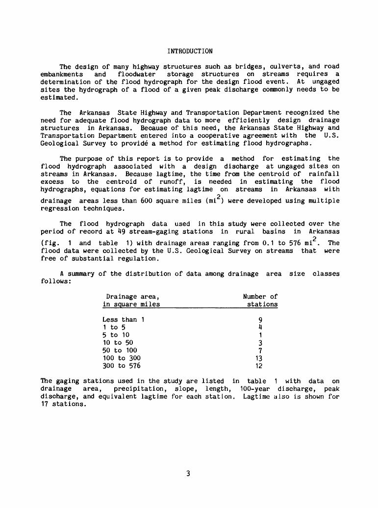
The design of many highway structures such as bridges, culverts, and road embankments and floodwater storage structures on streams requires a determination of the flood hydrograph for the design flood event. At ungaged sites the hydrograph of a flood of a given peak discharge commonly needs to be estimated.

The Arkansas State Highway and Transportation Department recognized the need for adequate flood hydrograph data to more efficiently design drainage structures in Arkansas. Because of this need, the Arkansas State Highway and Transportation Department entered into a cooperative agreement with the U.S. Geological Survey to provide a method for estimating flood hydrographs.

The purpose of this report is to provide a method for estimating the flood hydrograph associated with a design discharge at ungaged sites on streams in Arkansas. Because lagtime, the time from the centroid of rainfall excess to the centroid of runoff, is needed in estimating the flood hydrographs, equations for estimating lagtime on streams in Arkansas with

2 drainage areas less than 600 square miles (mi ) were developed using multipleregression techniques.

The flood hydrograph data used in this study were collected over the period of record at 49 stream-gaging stations in rural basins in Arkansas

2 (fig. 1 and table 1) with drainage areas ranging from 0.1 to 576 mi . Theflood data were collected by the U.S. Geological Survey on streams that were free of substantial regulation.

A summary of the distribution of data among drainage area size classes follows:

Drainage area, Number of in square miles________________stations

Less than 1 91 to 5 45 to 10 110 to 50 350 to 100 7100 to 300 13300 to 576 12

The gaging stations used in the study are listed in table 1 with data on drainage area, precipitation, slope, length, 100-year discharge, peak discharge, and equivalent lagtime for each station. Lagtime also is shown for 17 stations.

M1SSOUK1 9

193@C§QU*

19

^0.00

LOUISIANA

Figure 1. Location of study area

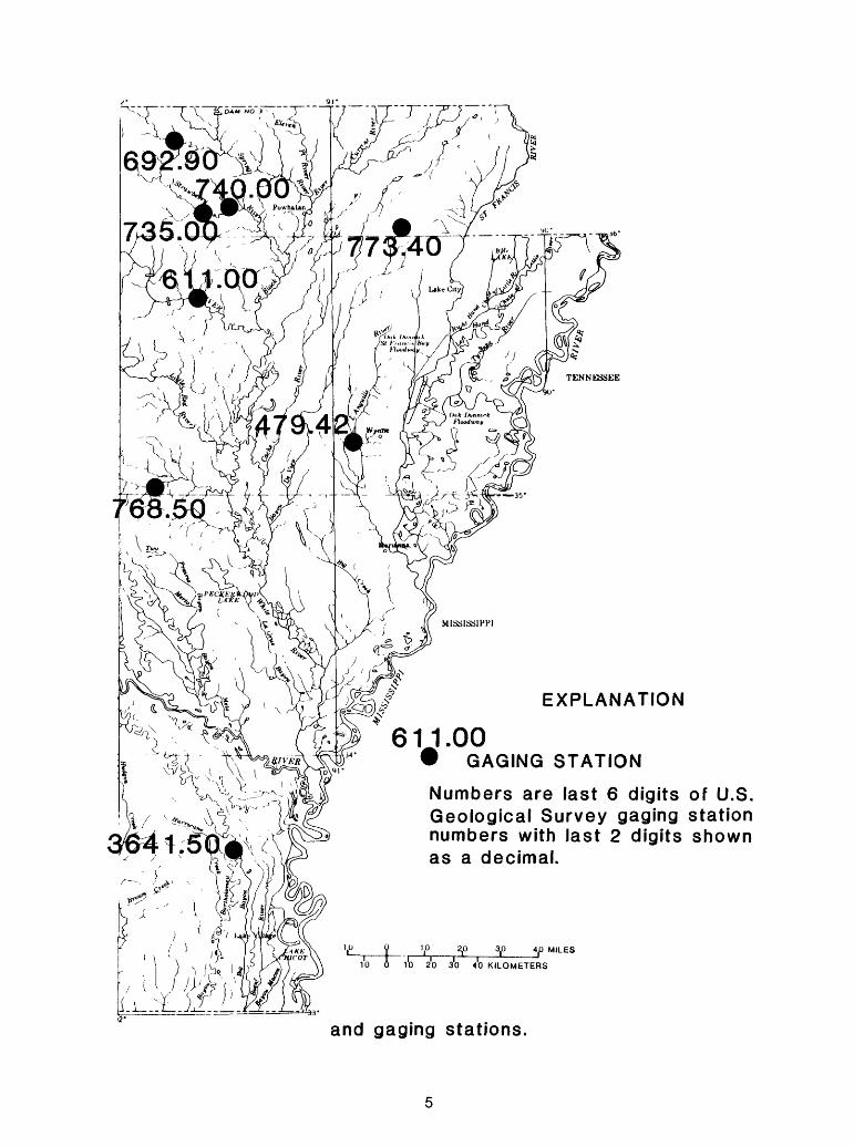
EXPLANATION

611.00 GAGING STATION

Numbers are last 6 digits of U.S. Geological Survey gaging station numbers with last 2 digits shown as a decimal.

10 30 30 40 MILES 10 0 1'0 2'0 3'0 40 KILOMETERS

and gaging stations.

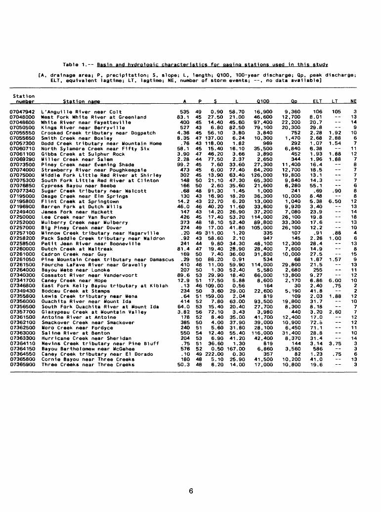
Table 1.-- Basin and hvdrologic characteristics for gaging stations used In this study

[A, drainage area; P, precipitation; S, slope; L, length; Q100. 100-year discharge; Qp, peak discharge; ELT, equivalent lagtlme; LT, lagtlme; NE, number of storm events; --, no data available]

Station number

07047942070480000704860007050500070555500705565007057300070607100706110007069290070735000707400007075000070753000707685007077340071950000719580007196900072494000725000007252000072570000725710007258200072585000726000007261000072610500726150007264000073403000734170007346800073494300735580007356000073565000735770007361500073621000736250007363000073633000736411007364150073645500736580007365900

Station name

L'Anguille River near ColtWest Fork White River at GreenlandWhite River near FayettevilleKings River near BerryvllleCrooked Creek tributary near DogpatchSmith Creek near Box leyDodd Creek tributary near Mountain HomeNorth Sylamore Creek near Fifty SixGibbs Creek at Sulphur RockMiller Creek near SalemPiney Creek near Evening ShadeStrawberry River near PoughkeepsieMiddle Fork Little Red River at ShirleySouth Fork Little Red River at ClintonCypress Bayou near BeebeSugar Creek tributary near WalcottOsage Creek near Elm SpringsFlint Creek at SpringtownBarren Fork at Dutch MillsJames Fork near HackettLee Creek near Van BurenMulberry Creek near MulberryBig Piney Creek near DoverMinnow Creek tributary near HagarvillePack Saddle Creek tributary near NaldronPetit Jean River near BoonevllleDutch Creek at NaltreakCadron Creek near GuyPine Mountain Creek tributary near DamascusFourche LaFave River near GravellyBayou Meto near LonokeCossatot River near VandervoortCaney Creek near HopeEast Fork Kelly Bayou tributary at KiblahBodcau Creek at StampsLewis Creek tributary near MenaOuachita River near Mount IdaSouth Fork Ouachita River at Mount IdaGlazypeau Creek at Mountain ValleyAntoine River at AntoineSmackover Creek near SmackoverMoro Creek near FordyceSaline River at BentonHurricane Creek near SheridanNevlns Creek tributary near Pine BluffBayou Bartholomew near McGeheeCaney Creek tributary near El DoradoCornie Bayou near Three CreeksThree Creeks near Three Creeks

A

53583.1400527

4.368.35.76

58.13.902.2899.2473302148166.68130

14.246.0147426373274.20.92241

81.4169.29410207

89.612.9.13234.6441464.03.82178385240550204.75576.10180

50.3

P

49454543454743454744454545505048434346434548494943444750504650535146505152535652505154535152494848

S

0.9027.5014.406.80

56.10137.00118.0015.4046.2077.507.606.0013.9021.102.60

91.3016.9022.7040.2014.2017.4018.1017.00

311.0058.609.8019.407.40

88.2011.001.30

29.9017.50

109.003.60

159.007.8015.4072.108.404.005.6012.406.9036.600.50

222.005.106.20

L

58.7021.0045.6082.503.806.241.82

16.103.662.37

33.6077.4063.4047.3035.601.45

18.206.2011.6026.9053.2052.4041.801.202.10

34.3028.9036.000.9159.9052.4018.405.880.5629.002.04

63.0020.403.4335.0037.9031.8055.4041.201.30

167.000.3025.9014.00

0100

16.90046,60097,40079,1003,84010,300

96935,5003,8902,650

27,30084,200126,00065,30021,6001,000

36,30013,00033,60037 , 200114,00089 , 800105,000

335947

48,10028,40031,800

534114,0005,580

66,0008,600

16422,600

81993.50027 , 7003,980

41,70039,00028,100116,00042,400

8196,860

35741,50017,000

9122220

1

6

11121996

10197

263326

12710

292

132

5

198

12106

318

3

1010

Oo

,360,700,200,300752,470292,840452344,400,700,800,840,280241,000.040.920.080,100,300,100107145.300,600,00068

,800,680.800,17030

,190109

,800,300440,400,900,450,400,370144,56082

,200,800

ELT

1068.0120.729.82.282.681.076.381.931.9616.418.513.114.355.1.69

8.485.383.4023.919.817.612.2.91

2.2628.414.927.51.8721.5255

9.276.862.4041.82.0331.78.183.2017.072.o71.128.831.43.145861.2341.019.6

LT

105------

1.922.881.54

--1.881.88

----------.90--

6.50----------.88

1.00------

1.57------

6.00.75--

1.88----

2.60----------

3.75--.75----

NE

3131491067

111278777688

12131418131046

138

1591311121022

1210771212111014336133

DIMENSIONLESS HYDROGRAPH METHOD

Inman (1986) used 355 actual (observed) streamflow hydrographs from 80 basins in Georgia, and harmonic analysis as described by O'Donnell (1960), to develop unit hydrographs. The 80 basins represented both urban and rural

2 streamflow characteristics and had drainage areas less than 20 mi . Anaverage unit hydrograph and an average lagtime were computed for each basin. These average unit hydrographs were then transformed to unit hydrographs having generalized durations of one-fourth, one-third, one-half, and three- fourths lagtime, then reduced to dimensionless terms by dividing the time by lagtime and the discharge by peak discharge. Representative dimensionless hydrographs developed for each basin were combined to generate one typical (average) dimensionless hydrograph for each of the four generalized durations. Using the four generalized duration dimensionless hydrographs, average basin lagtime, and peak discharge for each observed hydrograph, simulated hydro- graphs were generated for each of the 355 observed hydrographs, and their widths were compared with the widths of the observed hydrographs at 50 and 75 percent of peak flow. Inman (1986) concluded that the dimensionless hydro- graphs based on the one-half lagtime duration provided the best fit of the observed data. At the 50 percent of peak flow width, the standard error of estimate was + 31.8 percent; and at the 75 percent of peak flow width, the standard error of estimate was +35.9 percent.

For verification, the one-half lagtime duration dimensionless hydrograph was applied to 138 hydrographs from 37 Georgia stations that were not used in

2its development. Drainage areas of these stations ranged from 20 to 500 mi .Inman (1986) reported that at 50 percent of peak flow, the standard error of estimate of the width was ±39.5 percent and at 75 percent of peak flow, the standard error of estimate of the width was ±43.6 percent.

Inman (1986) performed a second verification to assess the total or cumulative prediction error for large floods through the combined use of the dimensionless hydrograph, estimated lagtimes from regional lagtime equations, and peak discharges from regional flood-frequency equations. He found standard errors of prediction of + 51.7 and + 57.1 percent for peak flow widths at 50 percent and 75 percent of peak flow, repectively.

On the basis that Inman's dimensionless hydrograph was developed and tested for a variety of conditions (small and large drainage basins in urban, rural, mountainous, and coastal plain areas) and has been shown by Robbins (1986) to be applicable to central Tennessee, it was theorized that it may be applicable to streams in Arkansas (C.R. Gamble, U.S. Geological Survey, written comm., 1989).

TESTING THE DIMENSIONLESS HYDROGRAPH FOR ARKANSAS STREAMS

A dimensionless hydrograph was developed for each of 17 gaging stations in Arkansas using data from 6 to 12 flood events at each site. The dimensionless hydrograph for each flood event was developed by dividing the discharge ordinate (Q) by the peak discharge (Q ) and by dividing the time (t)

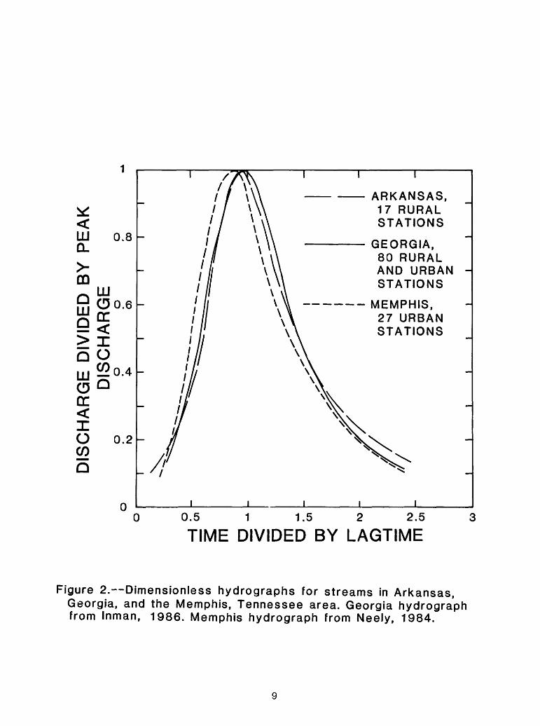
abscissa by the lagtime (LT). Zero time for flood events was the beginning of rainfall. The average dimensionless hydrograph for each station was con­ structed by aligning the peaks of each hydrograph and averaging the ordinate of discharge. The statewide dimensionless hydrograph was developed by the same averaging procedure using the diraensionless hydrographs for the 17 stations. The dimensionless hydrograph for Arkansas streams was similar to those developed for streams in Georgia (Inman, 1986) and in Memphis, Tennessee (Neely, 1984) as shown in figure 2. The time scale of the Memphis hydrograph is about 10 percent less than the time scale of the Arkansas and Georgia hydrographs but if the peaks on all the hydrographs are aligned, the hydrographs are very similar in shape.

The Arkansas dimensionless hydrograph was developed using actual hydrographs that included base flow whereas the Georgia dimensionless hydrograph was developed from several unit hydrographs that excluded base flow. For this reason the leading and trailing edges of the Arkansas dimensionless hydrograph are higher than those of the Georgia hydrograph. Also, the storm duration was assumed to be equal to one-half of the lagtirae for the Georgia hydrographs whereas the duration of the actual storms was used to prepare the dimensionless hydrograph for streams in Arkansas.

The Georgia diraensionless hydrograph was developed using more stations and is smoother in shape than the Arkansas hydrograph. For this reason, the dimensionless hydrograph used in this study is the one developed for Georgia streams by Inman (1986). The exclusion of base flow in the Georgia hydrograph is not a problem because this low part of the hydrograph corresponds to streamflow conditions below bankfull stage on most streams. The dimensionless hydrograph developed by Inman (1986) was verified by data from 17 stations in Arkansas. The Georgia diraensionless hydrograph was based on data for rural and urban streams, however, the 17 Arkansas stations used to verify the hydro- graph were rural streams. Although no urban Arkansas streams were available for verification, the diraensionless hydrograph presented in this report can be used for both rural and urban streams in Arkansas. A dimensionless hydrograph developed using 27 urban stations in the adjacent Memphis, Tennessee, area is shown on figure 2 for comparison. The hydrograph for Memphis streams was developed by using the diraensionless unit hydrograph (Neely, 1984) and by assuming that duration was equal to one-half the lagtime.

The dimensionless hydrograph used for this study (Inman, 1986) has the shape of a typical hydrograph on streams in Arkansas. The dimensionless hydrograph is shown graphically on figure 2, and data are compiled in table 2. These data can be used to compute a typical hydrograph for a selected peak discharge by multiplying each discharge ordinate of the diraensionless hydro- graph by the peak discharge and multiplying each time abscissa by the lagtime.

LLJ QL

CO

I O COQ

0.8

0.6

9?> IQ OLLJ £ 0-4O oQC

0.2

00

I

ARKANSAS, 17 RURAL STATIONS

GEORGIA, 80 RURAL AND URBAN STATIONS

MEMPHIS, 27 URBAN STATIONS

0.5 1 1.5 2 2.5

TIME DIVIDED BY LAGTIME

Figure 2. Dimensionless hydrographs for streams in Arkansas, Georgia, and the Memphis, Tennessee area. Georgia hydrograph from Inman, 1986. Memphis hydrograph from Neely, 1984.

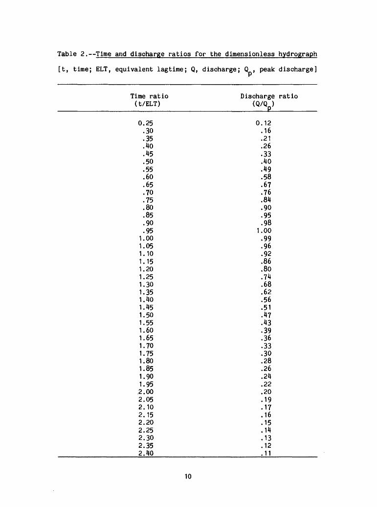
Table 2. Time and discharge ratios for the dimensionless hydrograph

[t, time; ELT, equivalent lagtime; Q, discharge; Q , peak discharge]

Time ratio (t/ELT)

0.25.30.35.40.45.50.55.60.65.70.75.80.85.90.95

1.001.051.101.151.201.251.301.351.401.451.501.551.601.651.701.751.801.851.901.95.2.002.052.102.152.202.252.302.352.40

Discharge ratio (Q/Qp )

0.12.16.21.26.33.40.49.58.67.76.84.90.95.98

1.00.99.96.92.86.80.74.68.62.56.51.47.43.39.36.33.30.28.26.24.22.20.19.17.16.15.14.13.12.11

10

ESTIMATING EQUIVALENT LAGTIME

Lagtime is defined as the time between the centroid of rainfall excess and the centroid of runoff. Lagtime (LT) for 17 stations in Arkansas (table1) was computed using the equation, LT = KSW + 0.5 T where KSW is thecrecession coefficient and T is the time base of the hydrograph as computed by

C

the rainfall-runoff model developed by Dawdy and others (1972) and modified by Carrigan (1973). If lagtime, peak discharge, and a dimensionless hydrograph are known, a hydrograph can be estimated for an ungaged site.

It is difficult to accurately determine the lagtime at some sites in the State for the following ' reasons. The time when the centroid of rainfall excess occurs may not be accurately defined because data from National Weather Service rain gages are usually recorded at 1-hour intervals. In addition, the rainfal?. measured at the rain gage may not be representative of the rainfall in the basin due to spatial variability of precipitation. Therefore, if data are insufficient for computation of the lagtime, an equivalent lagtime (ELT) can be estimated by the method described below.

Equivalent lagtime (ELT) is computed using data from an actual discharge hydrograph with the dimensionless hydrograph (fig. 2). Because it is impos­ sible to reproduce an actual discharge hydrograph in its entirety using one value of equivalent lagtime, it was decided to reproduce it for only a few points. The three selected points chosen and the appropriate equations for computing ELT at each point are as follows:

1. Width (in time) of the hydrograph at 75 percent of peak discharge.ELT = width/0.55 (1)

2. Width (in time) of the hydrograph at 50 percent of peak discharge.ELT = width/0.91 (2)

3. Width (in time) of the hydrograph between 50 percent of peak dis­ charge (rising stage) and 75 percent of peak discharge (falling s tafite)

ELT = width/0.69 (3)

From an actual discharge hydrograph, a value of ELT is computed using each of the three equations. If the values of ELT computed using the three equations are about the same, the arithmetic average can be used. If they differ, it is probably because the leading or trailing edge of the hydrograph is not typical and the ELT computed by equation 1 should be used.

The constants in the three equations were computed from the dimensionless hydrograph in table*2. Each constant was determined by subtracting the value of t/ELT on the rising limb of the dimensionless hydrograph from the value of t/ELT on the falling limb of the hydrograph at the appropriate discharge ratio, Q/Q .

The computation of ELT in this manner includes the different durations of the flood events used. In order to determine the average or typical hydro- graph, the ELT computed from several hydrographs at a station are averaged.

11

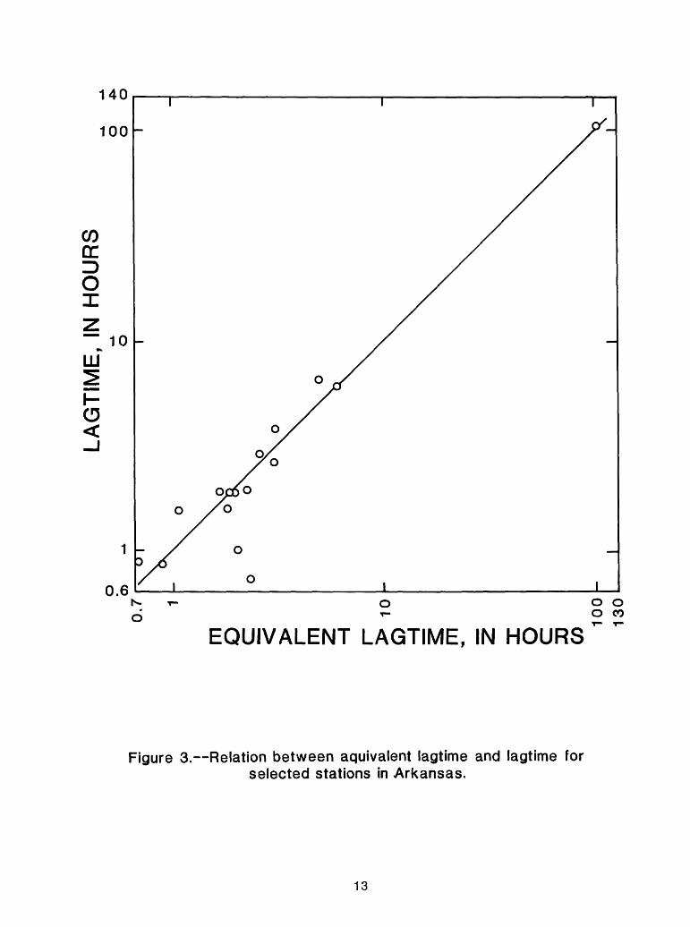
The ELT that is computed for a given discharge hydrograph may not be the actual lagtime, but it is the value that can be used to reproduce the actual discharge hydrograph from the dimensionless hydrograph. The lagtime and the ELT for the 17 stations in Arkansas used in defining the dimensionless hydro- graph are plotted on figure 3. The plot shows some scattering of the points but a relation does exist. Thus, ELT can be used to estimate hydrographs for selected peak discharge recurrence intervals.

At each gaging station listed in table 1, ELT was determined for each of several storm events. A total of 450 storm events was used for the 49 stations. Because some stations had many storm events while others had only a few, it was decided to compute an average ELT for each station rather than including all 450 storm events that could bias the results toward stations that had more storm events. At each station an average peak discharge of the storm events and an average ELT were determined and are shown in table 1. The average peak discharge of the storm events is the arithmetic average of the peak discharges of each storm event. The average ELT is the arithmetic average of the ELTs of each storm event.

Regression Analysis

The equivalent lagtime determined for the gaging stations used in the analysis was related to basin, climatic, and hydrologic parameters using linear multiple-regression techniques. The regression equation has the form:

v A b1 <5b2T b3 /i, \ Y = aA S L , (4)where, Y = equivalent lagtime,

A, S, and L are basin, climatic, and hydrologic characteristics, and a, t>1, b2, b3 are constants and coefficients obtained by regression analysis.

Regression analysis of the data indicates that drainage area and 100-year discharge are statistically significant characteristics (at the 95 percent confidence limit) for estimating ELT. The following equation was developed by the multiple regression technique using data from 49 gaging stations in Arkansas. The 100-year discharge is used so that one equation can be used throughout the State even though Arkansas has considerable variation in topography. The equation for computing ELT is shown below with the standard error of estimate.

ELT = 3,480 A 1 * 15Q100" 1>04± 38 percent (5)

where, ELT = the equivalent lagtime, in hours, used with the dimensionless hydrograph to reproduce an average discharge hydrograph.

2 A = the contributing drainage area of the basin, in mi , ando

Q IOQ= the discharge, in ffys for the 100-year flood (Neely, 1987).

12

140

100

CO DC

10

LLJ

1I- O

0.6o o o co

EQUIVALENT LAGTIME, IN HOURS

Figure 3. Relation between aquivalent lagtime and lagtime for selected stations in Arkansas.

13

Testing

The accuracy of the equation for estimating ELT is determined by computing the difference between the ELT values based on average station data (table 1) and the ELT values estimated by the regression equation. The accuracy, in percent, referred to as standard error, is the range of error that can be expected about two-thirds of the time. The standard error of regression of equation 5 is + 38 percent.

A test also was made to measure the accuracy of the ELT values obtained from the regression equation for large flood events. In this test, the largest flood of record was selected at each gaging station. The ELT was computed from the actual flood hydrographs by determination of the hydrograph widths at 50 and 75 percent of the peak discharges. The widths were used in equations 1 and 2 to compute the appropriate ELT values. These values of ELT were then compared with the ELT values computed using the regression equation. The standard errors at 50 and 75 percent of peak discharge were 41 and 39 percent, respectively.

The regression equation for equivalent lagtime also was tested for geographical bias and for variable bias. Geographical bias was tested by plotting the residuals on a State map. The residual is the computed ELT from station data divided by the computed ELT using the regression equation. The residuals were uniformly scattered on the plot and no geographical bias was observed. Each variable in the regression equation also was checked by residual analysis for bias. This was done by solving equation 5 for the particular variable being tested. The computed value was plotted on log-log paper against the variable being tested. If the variable being tested is unbiased, the plotted points should define a straight line with a slope equal to the exponent of the variable being tested. No bias was observed for any of the variables.

Sensitivity analyses were performed on the regression equation to measure the effect of errors in the independent variables (A, Q100 ) on the dependent

variable (ELT). All parameters were assumed to be constant except the one being tested for sensitivity; that parameter was assumed to contain an error ranging from +50 percent to -50 percent. The sensitivity of the regression equation to error in basin and hydrologic characteristics is shown below.

Percent Error in Computed ELT

Percent error in independent

variable

50 30 10

-10 -30 -50

A

59 35 12

-11 -34 -55

Q 100-34 -24 -9 12 45 106

14

For example, assume that the drainage area (A) for a particular site contains an error of +30 percent. That error would result in a 35 percent error in the computed ELT for the site using the regression equation. The percent error table shows that the equation is most sensitive to errors in drainage area (A) and 100-year discharge (

ESTIMATING FLOOD VOLUME

In some instances it is necessary to know the volume of runoff in the design of hydraulic structures. The following equation derived from this study can be used to determine the runoff volume for any typical flood event:

V = 0.00169 Q ELT

A (6)

where V is runoff volume, in inches, not including base flow;3 Q is peak discharge, in ft /s;

ELT is equivalent lagtime, in hours; and2 A is drainage area, in mi .

The constant in equation 6 was determined by summing the discharge ratio values in table 2 and adding estimated values for the leading and trailing edges of the hydrograph. This value was then multiplied by 3,600 (the numberof seconds in an hour) x 12 (the number of inches in a foot) x 0.05 (the time

p increment used in table 2) and divided by (5,280) (5,280 = the number of feetin a mile) .

HYDROGRAPH-WIDTH RELATION

For some design purposes, it is necessary to know only the period of time that a specific discharge will be exceeded. To provide this information, a hydrograph -width relation based on the dimensionless hydrograph was developed and is presented in table 3. The width ratio (W/ELT) was determined by subtracting the value of t/ELT on the rising limb of the dimensionless hydrograph from the value of t/ELT on the falling limb of the hydrograph at the same discharge ratio, Q/Q . The hydrograph width, W, can be estimated

for a specified discharge, Q, by first computing the ratio Q/Q and then

multiplying the corresponding W/ELT ratio by the equivalent lagtime, ELT.

APPLICATION OF HYDROGRAPH ESTIMATING TECHNIQUE

Suppose the shape of a typical hydrograph is needed for a site on Example Creek for the 25-year flood. The drainage area of the site is 22.4

2 mi , and the discharges of the 25- and 100-year floods have been determined

(Neely, 1987) to be 11,700 ft3/s and 18,000 ft3/s, respectively. From equation 5, a value of ELT is computed as:

ELT = 3,480 (22.4) 1 ' 15(18,000)~ 1 *°4 = 4.67 hours

15

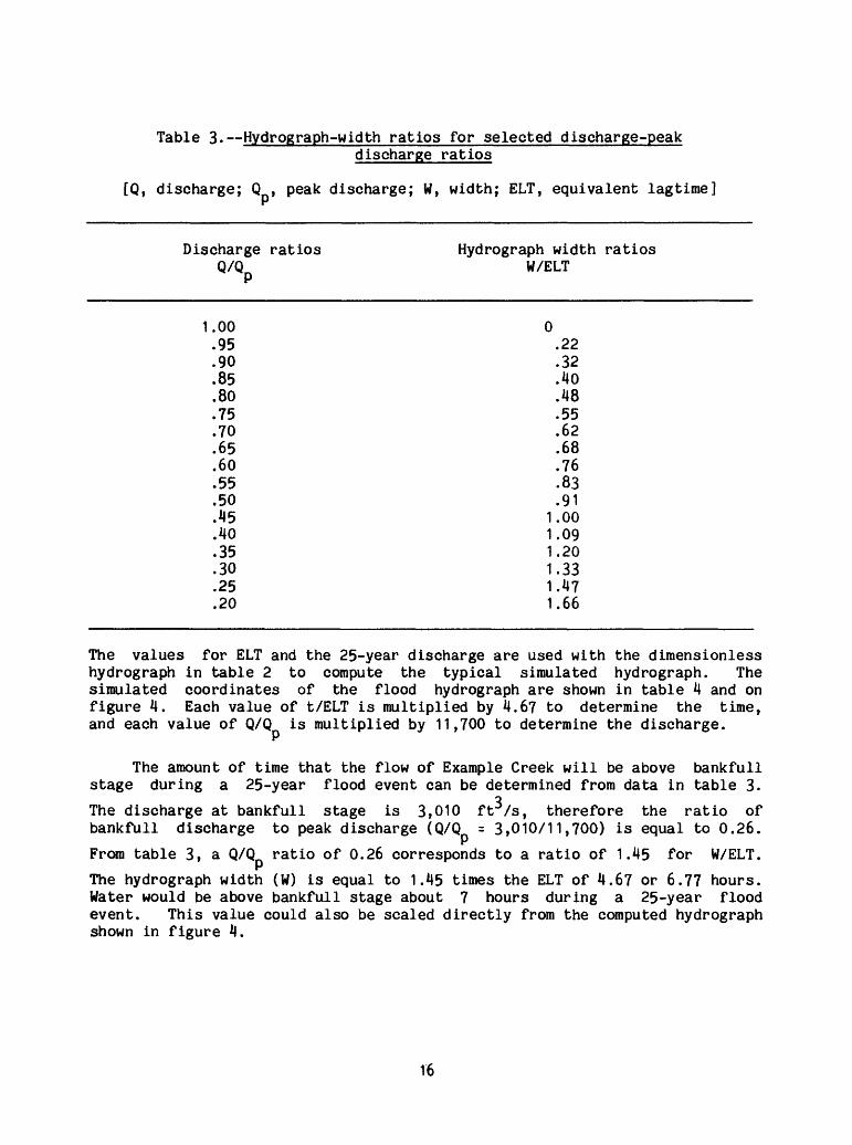
Table 3. Hydrograph-width ratios for selected discharge-peakdischarge ratios

[Q, discharge; Q , peak discharge; W, width; ELT, equivalent lagtime]

Discharge ratios Hydrograph width ratios Q/Q W/ELT

1.00.95.90.85.80.75.70.65.60.55.50.45.40.35.30.25.20

0.22.32.40.48.55.62.68.76.83.91

1.001.091.201.331.471.66

The values for ELT and the 25-year discharge are used with the dimensionless hydrograph in table 2 to compute the typical simulated hydrograph. The simulated coordinates of the flood hydrograph are shown in table 4 and on figure 4. Each value of t/ELT is multiplied by 4.67 to determine the time, and each value of Q/Q is multiplied by 11,700 to determine the discharge.

The amount of time that the flow of Example Creek will be above bankfull stage during a 25-year flood event can be determined from data in table 3.

QThe discharge at bankfull stage is 3,010 ft /s, therefore the ratio of bankfull discharge to peak discharge (Q/Q = 3,010/11,700) is equal to 0.26.

From table 3, a Q/Q ratio of 0.26 corresponds to a ratio of 1.45 for W/ELT.

The hydrograph width (W) is equal to 1.45 times the ELT of 4.67 or 6.77 hours. Water would be above bankfull stage about 7 hours during a 25-year flood event. This value could also be scaled directly from the computed hydrograph shown in figure 4.

16

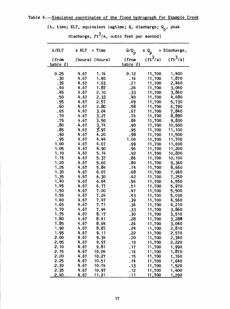
Table 4. Simulated coordinates of the flood hydrograph for Example Creek

[t, time; ELT, equivalent lagtime; Q, discharge; Q , peak

3 discharge, ft /s, cubic feet per second]

t/ELT

(from table 2)

0.25.30.35.40.45.50.55.60.65.70.75.80.85.90.95

1.001.051.101.151.201.251.301.351.401.451.501.551.601.651.701.751.801.851.901.952.002.052.102.152.202.252.302.352.40

x ELT = Time

(hours) (hours)

4.674.674.674.674.674.674.674.674.674.674.674.674.674.674.674.674.674.674.674.674.674.674.674.674.674.674.674.674.674.674.674.674.674.674.674.674.674.674.674.674.674.674.674.67

1.161.401.631.872.102.332.572.803.043.273.503.74£974.204.444.674.905.145.375.605.846.076.306.546.777.007.247.477.717.948.178.418.648.879.119.349.579.81

10.0410.2710.5110.7410.9711.21

Q/Qp

(from table 2)

0.12.16.21.26.33.40.49.58.67.76.84.90.95.98

1.00.99.96.92.86.80.74.68.62.56.51.47.43.39.36.33.30.28.26.24.22.20.19.17.16.15.14.13.12.11

x Q = Discharge,

(ft3/s) (ft3/s)

11,70011,70011,70011,70011,70011,70011,70011,70011,70011,70011,70011,70011,70011,70011,70011,70011,70011,70011,70011,70011,70011,70011,70011,70011,70011,70011,70011,70011,70011,70011,70011,70011,70011,70011,70011,70011,70011,70011,70011,70011,70011,70011,70011.700

1,4001,8702,4603,0403,8604,6805,7306,7907,8408,8909,830

10,50011,10011,50011,70011,60011,20010,80010,1009,3608,6607,9607,2506,5505,9705,5005,0304,5604,2103,8603,5103,2833,0402,8102,5702,3402,2201,9901,8701,7601,6401,5201,4001.290

17

h-ULJ LU

12

1 1

i£ 10m8 .Li.O co Q

io < oCO LJUZ> COo

8

LJLJ O DC

O COQ

85 50.

4

3

2

1

00

BANKFULL STAGE

34567

TIME, IN HOURS8 10

Figure 4. Simulated flood hydrograph for Example Creek.

18

SUMMARY

A dimensionless hydrograph is presented for Arkansas streams havingp

drainage areas less than about 600 mi . This dimensionless hydrograph can beused with peak discharge and equivalent lagtime to determine flood hydrographs at ungaged sites on rural and urban streams in Arkansas.

Multiple regression analysis was used to define relations between equivalent lagtime and basin, climatic, and hydrologic characteristics. Data collected on 450 storms at 49 gaging stations were used in the analysis. The regression analysis indicated that drainage area and 100-year discharge are significant parameters for estimating equivalent lagtime. The standard error of the regression equation is + 38 percent. The equation was tested for accuracy, bias, and sensitivity.

An equation Is presented for computing the volume of flood runoff when the peak discharge, equivalent lagtime, and drainage area are known. In addition, a hydrograph-width relation is presented for estimating the length of time that a specific discharge will be exceeded.

REFERENCES

Carrigan, P.H., Jr., 1973, Calibration of U.S. Geological Survey rainfall- runoff model for peak flow synthesis natural basins: U.S. Geological Survey open-file report, 109 p.

Carrigan, P.H., Dempster, G.R., and Bower, D.E., 1977, User's guide for U.S. Geological Survey rainfall-runoff model revision of Open-File Report 74- 33: U.S. Geological Survey Open-File Report 77-884, 273 p.

Dawdy, D.R., Lichty, R.W., and Bergmann, J.M., 1972, A rainfall-runoff simulation model for estimation of flood peaks for small drainage basins: U.S. Geological Survey Professional Paper 506-B, 28 p.

Inman, E.J., 1986, Simulation of flood hydrographs for Georgia streams: U.S. Geological Survey Water-Resources Investigations Report 86-4004, 41 p.

Neely, B.L., Jr., 1984, Flood frequency and storm runoff of urban areas of Memphis and Shelby County, Tennessee: U.S. Geological Survey Water- Resources Investigations Report 84-4110, 51 p.

1987, Magnitude and frequency of floods in Arkansas: U.S. Geological Survey Water-Resources Investigations Report 86-4335, 51 p.

O'Donnell, Terrance, 1960, Instantaneous unit hydrograph derivation by harmonic analysis: Commission of Surface Waters, Publication 51, International Association of Scientific Hydrology, p. 546-557.

Robbins, C.H., 1986, Techniques for simulating flood hydrographs and estimating flood volumes for ungaged basins in central Tennessee: U.S. Geological Survey Water-Resources Investigations Report 86-4192, 32 p.

U.S. GOVERNMENT PRINTING OFFICE; 1989 648-137/00014

19