Water Pipe Networks

Water Distribution Analysis Via Excel

Lecture 2

Pipe Network Definition Before Discussing How to Solve the Flow in Pipe Network,

Let’s Define the Following:

-Pipe;

-Node;

-Loop;

-Demand and Supply (QJ).

QJ1 QJ3 QJ5

QJ4

QJ6

QJ7

Objective of this Session •The objective of this session is to examine the use of

Excel to analyze a water distribution network.

•Excel is a commonly available spreadsheet package

that has been widely used as a computational tool in

almost all engineering applications.

Despite the demonstrated examples are simple, they

enables trainees to analyze realistic applications

while still requiring manual development of the

governing equations to reinforce the underlying

engineering principles.

•It is also believed that such full understanding should

come first and before getting first hand on the

application of commercial pipe network package.

Progress in Network Analysis

• Pre Computer Age:

- Graphical approaches:

- Hardy Cross Developed his famous method of

solving pipe networks in 1936.

• The Dawn of the Computer Age:

- In 1957, Hoag and Weinberg adapted Hardy Cross

approach in digital computers.

• Advanced Computer Methods

Steps of Network Analysis

In order to hydraulically analyze a given network, two

steps should be conducted:

-Step 1: Formulation of the governing equations;

-Step 2: Numerical solution of the obtained

equations.

Formulation of Network Equations Different approaches are found in the literature for the formulation

of the network equations. Examples of these approaches are:

-Using Junction equations;

-Using loop equations;

-Using pipe equations;

-Using a mix.

Based on the above approaches, the following methods have

been developed:

Q-Method: Solving for Pipe flows as unknowns (Qp);

H-Method: Solving for Heads at junctions as unknowns (HJ);

DQ-Method: Solving for Corrective flow rates as unknowns

(DQp) where: (Qp=Qo±DQp), Qo is a previous pipe flow guess;

DH-Method: Corrective heads at nodes as unknowns (DHj)

where: (Hj=Ho±DHj), Ho is a previous nodal head guess.

Solution of Network Equations The resulted governing equations are nonlinear (continuity

equations are linear whereas energy equations or loop equations

are non-linear) thus we need methods to solve non-linear

equations. Such methods include:

By iteration using some correction formula (such as HCM);

By minimization of a target function (we could use Excel solver);

By linearization to convert equations into linear equations then

use matrix manipulation for this regard with some iterations;

Direct solution of non-linear equations by using Newton-

Raphson method.

Example of Q-Method

List all the governing equations to solve the below

network using the Q-method.

Five Equations in

Five Unknowns

Formulation of Network Equations

H-Method

Example of H-Method

Q12=Q23+QJ2 Q12-Q23 = QJ2

Q12+Q13=QJ1 Q12+Q13=QJ1=QJ2 +QJ3

Q13+Q23 =QJ3 Q13+Q23 =QJ3

By using the Head expression and substitute back, the

above equations reduce to:

Three Equations in

Three Unknowns

QJ2

QJ3

QJ1

Hardy Cross Method (HCM)

1936Hardy Cross

The method was first published in November 1936 by Hardy

Cross, a structural engineering professor at the University of

Illinois at Urbana–Champaign.The Hardy Cross method is an

adaptation of the Moment distribution method, which was also

developed by Hardy Cross as a way to determine the moments in

indeterminate structures.

Example of DQ method

Governing Equations

1

4

3

6

2

5

Q12

Q45

Q23

Q56

Q36 Q14 Q25

qout2

qout1

qin1

Hardy Cross Method requires an initial guesses of all pipe

flows under the condition that such guesses satisfy the

conservation of mass at each node.

For example: Each Node We Could Write a Mass

Conservation Equation:

Example @ Node 2: Q12=qout1+Q23+Q25

a. Conservation of Mass (Nodal Equations)

Governing Equations

1

4

3

6

2

5

Q12

Q45

Q23

Q56

Q36 Q14 Q25

qout2

qout1

qin1

For Each closed Loop, the summation of head lost should vanish:

Example @ Loop 1: HL12+HL25+HL54+HL41

For Each Link We Could Write the head lost:

Example @ Link1-2: HL12= K12.Q12|Q12|

b. Conservation of Energy (Loop Equations)

Loop 1 Loop 2

Thus, For Loop 1: K12.Q12|Q12|+ K25.Q25|Q25|+ K54.Q54|Q54|+ K41.Q41|Q41|=0

25

8

gD

fLKWhere:

Solution Steps Using HCM Solution of Pipe Network via HCM is iterative as follow:

1. Consider a positive flow direction for all loops (say clock

wise direction is positive;

2. Assume flow discharges for all pipes satisfying the mass

conservation at each node;

3. Calculate a first approximation of the flow correction for

each loop using the following equation given by Hardy

Cross:

4. Calculate the corrected Q and iterate till corrections

vanish.

An Alternative Approach…

Using Excel Solver

An alternative approach to avoid using the flow correction

equation given by Hardy Cross is to directly use the Excel

Solver to obtain the suitable loop flow correction DQ that is

required to make the summation of the head losses across any

loop equal zero.

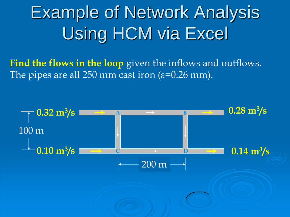
Example of Network Analysis

Using HCM via Excel

Find the flows in the loop given the inflows and outflows. The pipes are all 250 mm cast iron (e=0.26 mm).

A B

C D 0.10 m3/s

0.32 m3/s 0.28 m3/s

0.14 m3/s

200 m

100 m

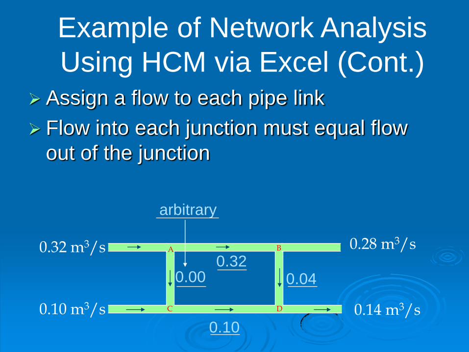
Assign a flow to each pipe link

Flow into each junction must equal flow

out of the junction

A B

C D 0.10 m3/s

0.32 m3/s 0.28 m3/s

0.14 m3/s

0.32 0.00

0.10

0.04

arbitrary

Example of Network Analysis

Using HCM via Excel (Cont.)

Example of Network Analysis Using

Hardy Cross Method

Calculate the head loss in each pipe

f=0.02 for Re>200000 hf

8 fL

gD5 2

Q

2

fh kQ Q=

339)25.0)(8.9(

)200)(02.0(8

251

k

k1,k3=339 k2,k4=169

A B

C D 0.10 m3/s

0.32 m3/s 0.28 m3/s

0.14 m3/s

1

4 2

3

hf1 34.7m

hf2 0.222m

hf3 3.39m

hf4 0.00m

hfi

i1

4

31.53m

Sign convention +CW

2

5

s

m

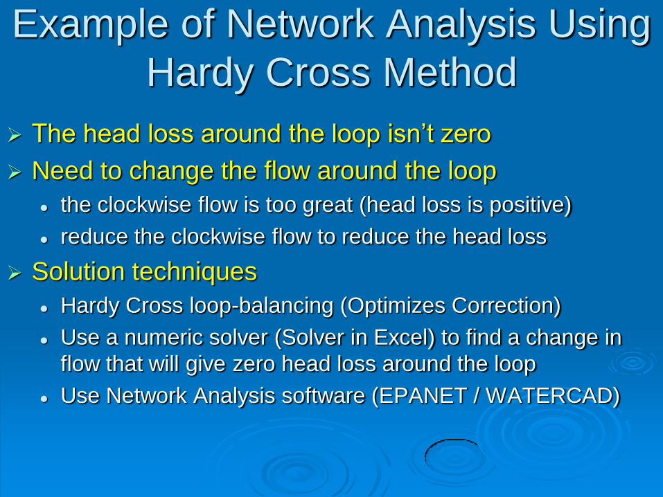
The head loss around the loop isn’t zero

Need to change the flow around the loop

the clockwise flow is too great (head loss is positive)

reduce the clockwise flow to reduce the head loss

Solution techniques

Hardy Cross loop-balancing (Optimizes Correction)

Use a numeric solver (Solver in Excel) to find a change in

flow that will give zero head loss around the loop

Use Network Analysis software (EPANET / WATERCAD)

Example of Network Analysis Using

Hardy Cross Method

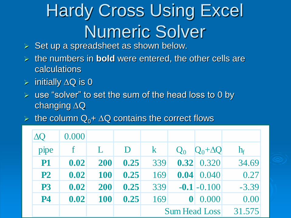
Hardy Cross Using Excel

Numeric Solver Set up a spreadsheet as shown below.

the numbers in bold were entered, the other cells are

calculations

initially DQ is 0

use “solver” to set the sum of the head loss to 0 by

changing DQ

the column Q0+ DQ contains the correct flows

∆Q 0.000

pipe f L D k Q0 Q0+∆Q hf

P1 0.02 200 0.25 339 0.32 0.320 34.69

P2 0.02 100 0.25 169 0.04 0.040 0.27

P3 0.02 200 0.25 339 -0.1 -0.100 -3.39

P4 0.02 100 0.25 169 0 0.000 0.00

31.575Sum Head Loss

Solution to Loop Problem

A B

C D 0.10 m3/s

0.32 m3/s 0.28 m3/s

0.14 m3/s

0.218

0.102

0.202

0.062

1

4 2

3

Q0+ DQ

0.218 0.062 0.202 0.102

Better solution is software with a GUI showing the pipe network.

Solution of A Single Loop Problem Using

HCM Via Excel (Video)

Solution of a Single Loop Problem with a

Pump Using HCM Via Excel (Video)

Solution of a Multiple Loops Problem

Using HCM Via Excel (Video)

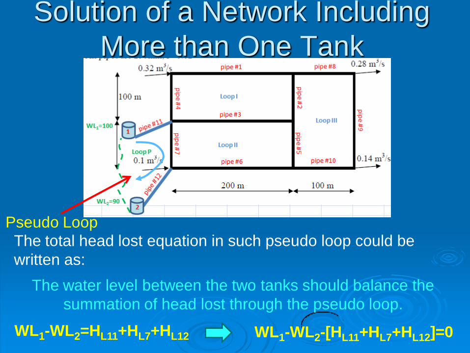
Solution of a Network Including

More than One Tank

The common practice is to form a pseudo loop that

includes the given tanks as follow:

Solution of a Network Including

More than One Tank

Pseudo Loop

The total head lost equation in such pseudo loop could be

written as:

The water level between the two tanks should balance the

summation of head lost through the pseudo loop.

WL1-WL2=HL11+HL7+HL12 WL1-WL2-[HL11+HL7+HL12]=0

Solution of a Network with Tanks- Pseudo

Loop Approach via HCM (Video)

Solving HCM Using Matrices

and Network Jacobian This method is also called as simultaneous

loops equations in terms of DQi;

The loops equations could be written as:

[J].{DQ} = {-SHL}

Jacobian of

Loops Network

Unknown Corrections of

Flow in Each Loop

(including Pseudo loops)

Nloops xNloops Nloops x1 Nloops x1

Negative Sum of

Head Lost in

Each Loop

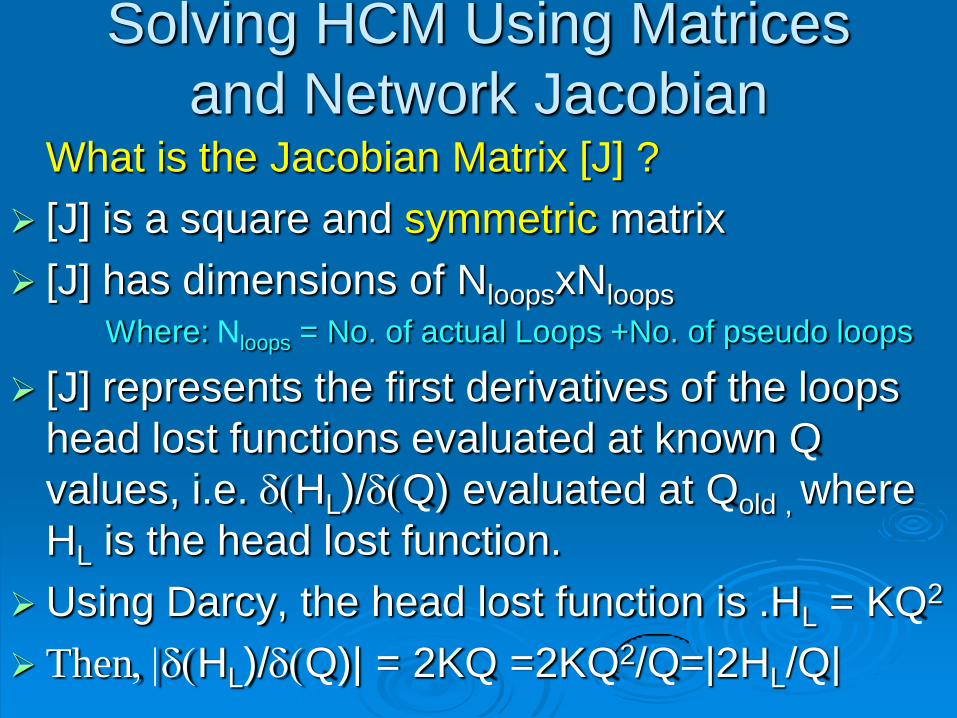
Solving HCM Using Matrices

and Network Jacobian What is the Jacobian Matrix [J] ?

[J] is a square and symmetric matrix

[J] has dimensions of NloopsxNloops

Where: Nloops = No. of actual Loops +No. of pseudo loops

[J] represents the first derivatives of the loops

head lost functions evaluated at known Q

values, i.e. d(HL)/d(Q) evaluated at Qold , where

HL is the head lost function.

Using Darcy, the head lost function is .HL = KQ2

Then, |d(HL)/d(Q)| = 2KQ =2KQ2/Q=|2HL/Q|

Solving HCM Using Matrices

and Network Jacobian

What is the Jacobian Matrix [J] ?

Accordingly, [J] could be written as:

Or,

Remember, [J] matrix is a symmetric matrix

Symmetric Non

Zero Elements

Solving HCM Using Matrices

and Network Jacobian

What is the Jacobian Matrix [J] ?

-The off-diagonal elements of the [J] matrix represent the

negative gradient of the head lost function for the pipes in

common between different loops?

- For instance: the term represents the negative

head-lost function for the pipe in common between loop 1 and

loop 2.

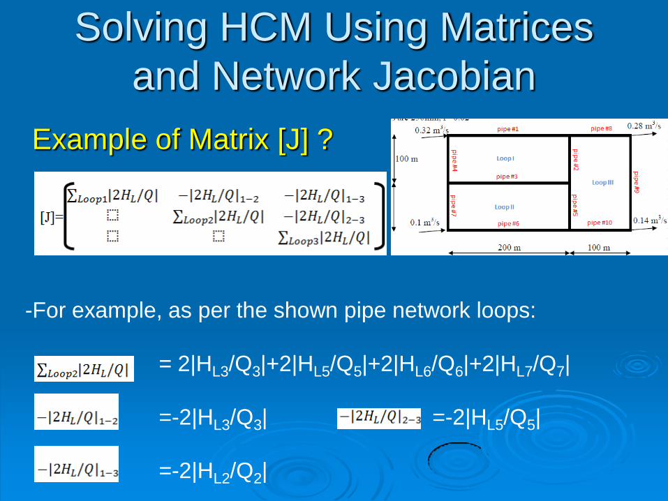
Solving HCM Using Matrices

and Network Jacobian

Example of Matrix [J] ?

-For example, as per the shown pipe network loops:

= 2|HL3/Q3|+2|HL5/Q5|+2|HL6/Q6|+2|HL7/Q7|

=-2|HL3/Q3| =-2|HL5/Q5|

=-2|HL2/Q2|

Solving HCM Using Matrices

and Network Jacobian

Creation of the Negative Sum of Head Lost

Vector {-SHL}:

For the shown three loops:

Solving HCM Using Matrices

and Network Jacobian The loops equations could be solved to get

the flow corrections DQ for each loop as

follow:

[J].{DQ} = {-SHL}

Using Matrix Inverse:

{DQ} =[J]-1 {-SHL}

Using Excel for Matrix

Manipulation Example 1: Matrix Multiplications:

Using Excel for Matrix

Manipulation Example 1: Matrix Multiplications (Cont.):

Using Excel for Matrix

Manipulation Example 1: Matrix Multiplications (Cont.):

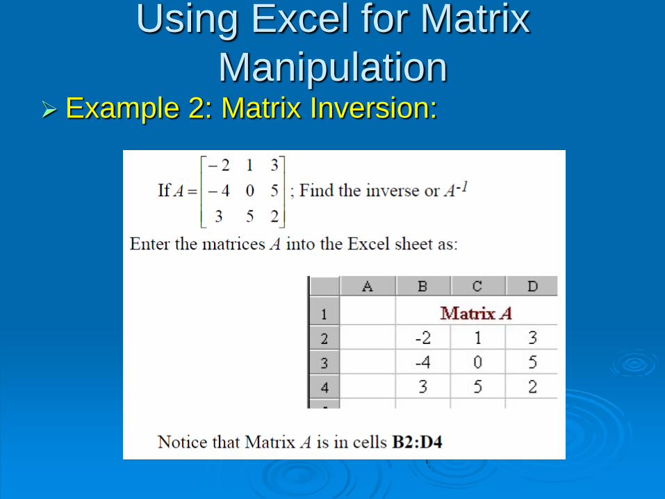
Using Excel for Matrix

Manipulation Example 2: Matrix Inversion:

Using Excel for Matrix

Manipulation Example 2: Matrix Inversion (Cont.):

Using Excel for Matrix

Manipulation Example 2: Matrix Inversion (Cont.):

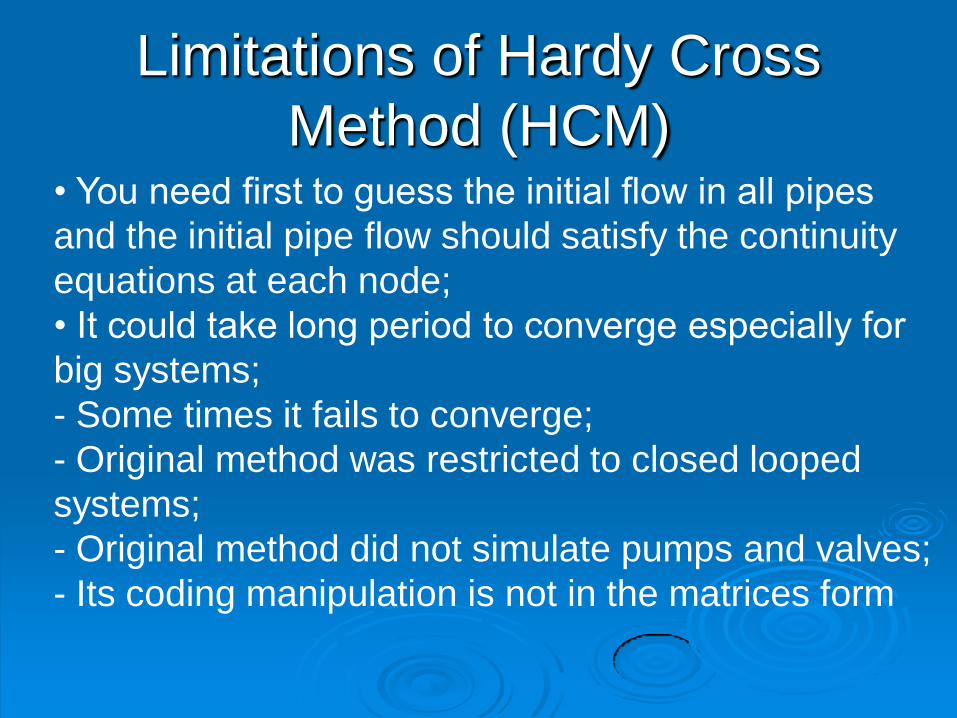
Limitations of Hardy Cross

Method (HCM) • You need first to guess the initial flow in all pipes

and the initial pipe flow should satisfy the continuity

equations at each node;

• It could take long period to converge especially for

big systems;

- Some times it fails to converge;

- Original method was restricted to closed looped

systems;

- Original method did not simulate pumps and valves;

- Its coding manipulation is not in the matrices form

Further Readings

Next Slides are out of scope of

Final Exam

Are there any other method that does not require initial flow guess

based on continuity and can be casted in a matrix form?

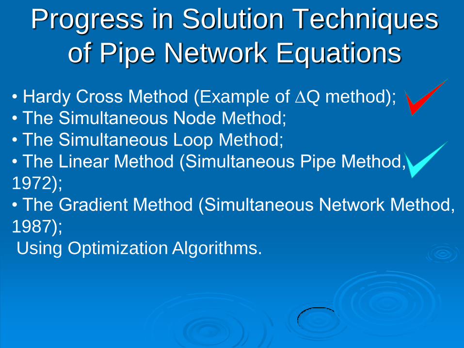
Progress in Solution Techniques

of Pipe Network Equations

• Hardy Cross Method (Example of DQ method);

• The Simultaneous Node Method;

• The Simultaneous Loop Method;

• The Linear Method (Simultaneous Pipe Method,

1972);

• The Gradient Method (Simultaneous Network Method,

1987);

Using Optimization Algorithms.

Solution of the Q-Method using

Linearization

Let’s formulate the governing equations of the given

network using the Q-method then let’s solve the

obtained equations using linearization.

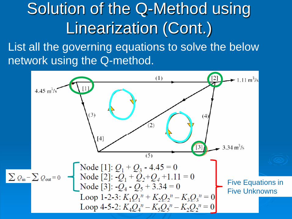
Solution of the Q-Method using

Linearization (Cont.) List all the governing equations to solve the below

network using the Q-method.

Five Equations in

Five Unknowns

Let us Look Carefully and Examine the Produced

Equations…

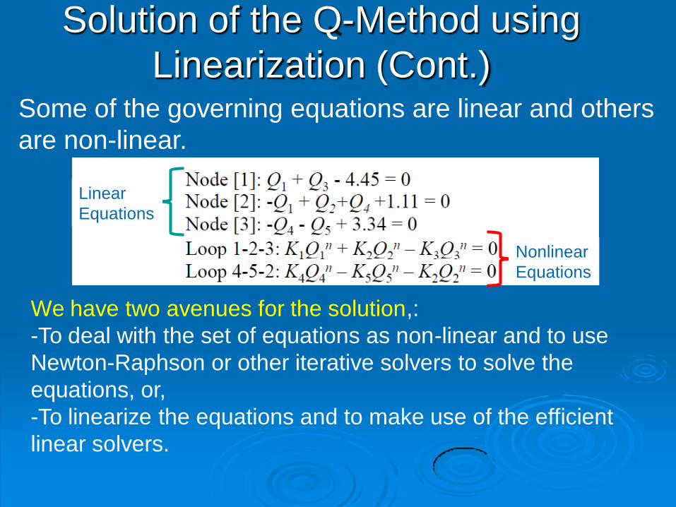
Solution of the Q-Method using

Linearization (Cont.) Some of the governing equations are linear and others

are non-linear.

Nonlinear

Equations

Linear

Equations

We have two avenues for the solution,:

-To deal with the set of equations as non-linear and to use

Newton-Raphson or other iterative solvers to solve the

equations, or,

-To linearize the equations and to make use of the efficient

linear solvers.

Let us Go with Linearization

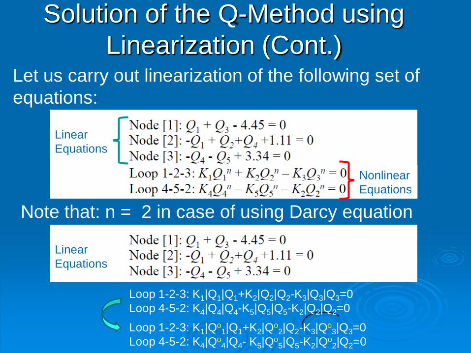
Solution of the Q-Method using

Linearization (Cont.) Let us carry out linearization of the following set of

equations:

Nonlinear

Equations

Linear

Equations

Note that: n = 2 in case of using Darcy equation

Linear

Equations

Loop 1-2-3: K1|Q1|Q1+K2|Q2|Q2-K3|Q3|Q3=0

Loop 4-5-2: K4|Q4|Q4-K5|Q5|Q5-K2|Q2|Q2=0

Loop 1-2-3: K1|Qo

1|Q1+K2|Qo

2|Q2-K3|Qo

3|Q3=0

Loop 4-5-2: K4|Qo

4|Q4- K5|Qo

5|Q5-K2|Qo

2|Q2=0

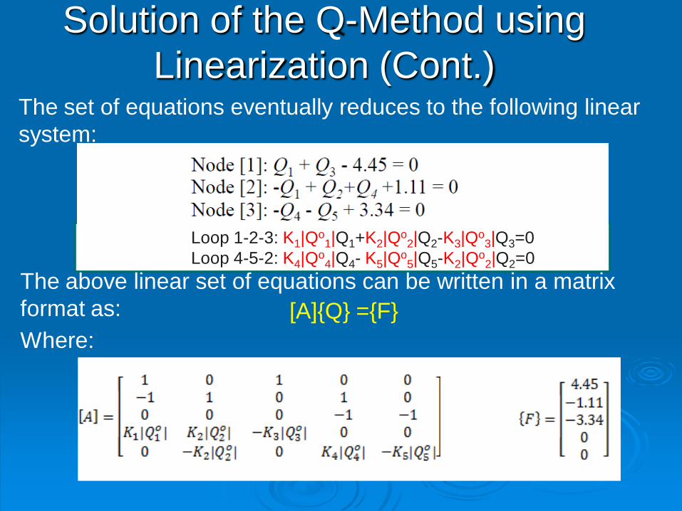
Solution of the Q-Method using

Linearization (Cont.) The set of equations eventually reduces to the following linear

system:

Loop 1-2-3: K1|Qo

1|Q1+K2|Qo

2|Q2-K3|Qo

3|Q3=0

Loop 4-5-2: K4|Qo

4|Q4- K5|Qo

5|Q5-K2|Qo

2|Q2=0

The above linear set of equations can be written in a matrix

format as: [A]{Q} ={F}

Where:

Solution of the Q-Method using

Linearization (Cont.) The value of the unknown {Qnew} can be obtained using iteration

as follow:

{Qnew} =[A] -1{F} & Qo =(Qoold+Qnew)/2

Where:

Transformation Matrix Force Vector

Or Demand Vector

Linearization via Excel (Video)