Water Ice and Dust in the Innermost Coma of Comet103P/Hartley 2

Silvia Protopapaa, Jessica M. Sunshinea, Lori M. Feagaa, Michael S. P. Kelleya,Michael F. A’ Hearna, Tony L. Farnhama, Olivier Groussinb, Sebastien Bessea,c,

Frederic Merlind, Jian-Yang Lie

aDepartment of Astronomy, University of Maryland, College Park, MD, 20742, USAbAix-Marseille Universite, CNRS, LAM (Laboratoire dAstrophysique de Marseille) UMR 7326,

13388, Marseille, FrancecESA/ESTEC, Keplerlaan 1, Noordwijk, The Netherlands

dUniversite Denis Diderot Paris 7, LESIA, Observatoire de Paris, FranceePlanetary Science Institute, Tucson, AZ 85719, USA

Abstract

On November 4th, 2010, the Deep Impact eXtended Investigation (DIXI) success-

fully encountered comet 103P/Hartley 2, when it was at a heliocentric distance of

1.06 AU. Spatially resolved near-IR spectra of comet Hartley 2 were acquired in

the 1.05 – 4.83 µm wavelength range using the HRI-IR spectrometer. We present

spectral maps of the inner ∼10 kilometers of the coma collected 7 minutes and

23 minutes after closest approach. The extracted reflectance spectra include well-

defined absorption bands near 1.5, 2.0, and 3.0 µm consistent in position, band-

width, and shape with the presence of water ice grains. Using Hapke’s radiative

transfer model, we characterize the type of mixing (areal vs. intimate), relative

abundance, grain size, and spatial distribution of water ice and refractories. Our

modeling suggests that the dust, which dominates the innermost coma of Hartley

2 and is at a temperature of 300K, is thermally and physically decoupled from the

fine-grained water ice particles, which are on the order of 1 µm in size. The strong

correlation between the water ice, dust, and CO2 spatial distribution supports the

Preprint submitted to icarus June 16, 2014

arX

iv:1

406.

3382

v1 [

astr

o-ph

.EP]

12

Jun

2014

concept that CO2 gas drags the water ice and dust grains from the nucleus. Once

in the coma, the water ice begins subliming while the dust is in a constant outflow.

The derived water ice scale-length is compatible with the lifetimes expected for

1-µm pure water ice grains at 1 AU, if velocities are near 0.5 m/s. Such velocities,

about three order of magnitudes lower than the expansion velocities expected for

isolated 1-µm water ice particles [Hanner, 1981; Whipple, 1951], suggest that the

observed water ice grains are likely aggregates.

Keywords:

Comets, Comets, coma, Comets, composition, Comets, dust, Ices

1. Introduction

Comets formed beyond the H2O frost line, where ices can condense [e.g.,

A’Hearn et al., 2012]. A variety of processes have affected comets during their

long storage in the Oort cloud and scattered disk (e.g., irradiation by energetic par-

ticles, heating by passing stars, collisions). Similarly, repeated solar heating leads

to evolution of short period comets during their many passages close to the Sun.

However, because most of these processes affect only the outer layer of comets,

the pristine nature of the bulk of the nucleus is preserved [Bockelee-Morvan et al.,

2004; Mumma et al., 1993; Stern, 2003; Weissman and Stern, 1997]. As such,

comets are excellent laboratories to extend our understanding of the origin and

evolution of the Solar System.

Given that comets contain the least processed primordial materials that formed

the cores of the giant planets [A’Hearn, 2011], the analysis of the composition and

physical state of cometary materials is critical to improve our understanding of the

accretion processes that led to the formation of comet nuclei and ultimately the

2

planets. Water is a key component of comets [Bockelee-Morvan et al., 2004;

Bockelee-Morvan and Rickman, 1997; Feaga et al., 2007; Mumma and Charnley,

2011] and water ice has been observed from the ground and with in situ obser-

vations in the comae [Davies et al., 1997; Kawakita et al., 2004; Sunshine et al.,

2011a; Yang et al., 2009], on the surfaces [Sunshine et al., 2006], and in the near-

surface interiors [Sunshine et al., 2007] of comets. An example of addressing

comet nuclei formation by means of water ice characteristics is given by Sunshine

et al. [2007]: the presence of very fine (∼1 µm) water ice particles in the im-

pact ejecta of comet Tempel 1, free of refractory impurities, led to question the

interstellar dust grain model proposed by Greenberg [1998] and Greenberg and Li

[1999]. The basic idea of this model is that comets formed directly through coag-

ulation of interstellar dust. As such, the morphological structure of comet nuclei is

an aggregate of presolar interstellar dust grains, which consist of a core of silicates

mantled first by a shell of organic refractory material and then by a mixture of wa-

ter dominated ices, which are embedded with thousands of very small (1-10 nm)

carbonaceous/large molecule particles. According to Sunshine et al. [2007], it is

unlikely that water ice would segregate from the superfine particles in the impact

ejecta. The model by Greenberg is only one of the several models proposed, de-

scribing the underlying structure of cometary nuclei (e.g., the “fluffy aggregate” of

Donn et al. [1985] and Donn and Hughes [1986], the “rubble pile model”, either

collisionally modified [Weissman et al., 2004] or primordial [Weissman, 1986],

the “icy-glue” model of Gombosi and Houpis [1986], the “talps” or “layered pile”

model by Belton et al. [2007]). All of these models consider different origins

and/or evolutionary processes. Investigations of cometary nuclei at close range,

which can only be achieved by space missions, are required to validate, disprove,

3

or improve these various formation models.

On November 4th, 2010, the Deep Impact Flyby (DIF) spacecraft [A’Hearn

et al., 2005; Hampton et al., 2005] successfully encountered comet 103P/Hartley

2 as part of its extended mission, the Deep Impact eXtended Investigation (DIXI)

[A’Hearn et al., 2011]. The DIF spacecraft employs two multi-spectral imagers

(MRI-VIS, HRI-VIS) and a 1.05 – 4.83 µm near-infrared spectrometer (HRI-IR).

Near-IR spectra of comet Hartley 2 were acquired for several weeks before and af-

ter closest approach (CA, at a range of 694 km, occurred on November 4th, 2010,

at 13:59:47.31 UTC with a maximum HRI-IR spatial resolution of 7 m/pixel).

DIXI observations revealed a bi-lobed, very small (maximum length of 2.33 km,

[A’Hearn et al., 2011]), and highly active nucleus, with water ice distributed het-

erogeneously, in specific areas on the surface [Sunshine et al., 2011b] and in the

coma [Protopapa et al., 2011; Sunshine et al., 2011a].

In this paper, we present a detailed analysis of the composition and texture

of water ice and refractories in the inner-most coma of Hartley 2, within a few

kilometers of the surface, using DI HRI-IR data. We investigate the physical

makeup of the water ice grains, with the goal of providing more observational

constraints to help us have a better understanding of the accretion process that led

to the formation of comet nuclei. We investigate the role of the gas in delivering

the water ice and dust to the coma of Hartley 2 and how the emitted material

evolves after it leaves the nucleus.

2. Observations

Spatially resolved near-IR spectra of comet Hartley 2 were acquired in the

1.05 – 4.83 µm wavelength range using the HRI-IR spectrometer [Hampton et al.,

4

2005]. HRI-IR data were collected from 01 October 2010 to 26 November 2010.

In this paper, only a subset of data is analyzed. In particular, we present HRI-

IR spatially resolved scans of comet Hartley 2 collected 7 (ID 5006000) and 23

(ID 5007002) minutes post-CA. Table 1 lists the main characteristics of these two

scans.

The IR data are calibrated using the DI science data pipeline [Klaasen et al.,

2008, 2013] and are available in the NASA Planetary Data System (PDS) archive

[McLaughlin et al., 2013]. The standard steps of the pipeline processing include

linearization, dark subtraction, flat fielding, conversion from DN to radiance units

(W m−2sr−1µm−1), and bad pixel masking. These data have been recalibrated

since the work by A’Hearn et al. [2011], although the differences are not dramatic.

The 5006000 and 5007002 radiance maps are shown in panels (a) and (b) of Figure

1, respectively, compared with the HRIVIS and MRI-VIS context images (with

characteristics given in Table 2). Because the HRI-IR instrument is a scanning

slit spectrometer, reconstructed spatial information is susceptible to errors from

jumps in spacecraft attitude due to impacting particles or autonomous operations.

A mismatch in the nucleus shape between the IR scan acquired 7 min post-CA and

the corresponding visible context images was observed, possibly caused by very

small grains hitting the spacecraft at high speed. We have corrected this mismatch

by shifting the bottom 14 rows of the 56-row IR scan by 1 pixel to the left and the

top 21 rows by 1 pixel toward the right and bottom (with respect to the orientation

of Figure 1).

Both the 5006000 and 5007002 scans contain the nucleus of Hartley 2 and

the surrounding coma. The nucleus is in roughly the same orientation in the two

scans. The precession of the long axis of the nucleus around the angular momen-

5

tum vector has a period of 18.4 hours at encounter [A’Hearn et al., 2011; Belton

et al., 2013]; therefore in 16 min separating the two scans, the rotation of the nu-

cleus is negligible with regards to coma studies, as is the change of the spacecraft

line of sight. In both scans, there are jets off the end of the smaller lobe of the

nucleus and beyond the terminator along the lower edge of the larger lobe (Figure

1).

The nucleus of Hartley 2 needs to be masked in order to focus our analysis

on the water ice and refractories in the inner-most coma. The dashed red line in

Figure 1 outlines the illuminated portion of the cometary nucleus, including the

scattered light near the limb, that is excluded from our analysis. This mask was

defined at long wavelengths (λ ≥ 3.5 µm), where the thermal emission of the

nucleus dominates over the signal from the dust in the coma, allowing the nucleus

and coma to be disentangled. The nucleus contour is defined by radiance values in

the 450 channel (∼4.1 µm) greater than 0.16 W m−2sr−1µm−1 in order to match

the nucleus as seen in the HRI-VIS and MRI-VIS images acquired at the same

time as the IR data.

3. Spectral Modeling

3.1. Reflectance

Once the flux is calibrated into radiance, I , from the pipeline, we can convert

it into reflectance, R, by

R(λ) =πI(λ)r2

F(λ)(1)

where F(λ) is the solar flux at 1 AU, and r is the heliocentric distance, in our

case 1.06 AU. The solar spectrum we use is a synthesized spectrum from various

6

sources [Berk et al., 2006; Kurucz, 1995], available at the MODTRAN web site

http://rredc.nrel.gov/solar/spectra/am0/other_spectra.html.

The next step of our analysis is the determination of the error on the radiance.

The derived error will be used in the best fit minimization of the reflectance spectra

(see Section 3.4). At each wavelength, the radiance map (see Figure 2, panel

a) is smoothed using a moving resistant mean in a 3×3 pixel box (see Figure

2, panel b). Outliers that vary by more than 2.5σ are excluded. The smoothed

radiance map is then subtracted from the original one, producing a background

noise map (see Figure 2, panel c) where coma structures are no longer visible,

except where the jets are particularly strong (e.g., jets originating from the lower

edge of the larger lobe of the nucleus). For each pixel of the background noise

map, the standard deviation of the mean of its neighboring pixels located in a

3-by-3 pixel box is computed and assumed to be the radiance error. A careful

examination of panel (c) in Figure 2 allows us to conclude that this approach can

be applied everywhere except for areas with coma structures that still remain in

the background map. Avoiding these areas we take the mean uncertainty of the

background at each wavelength (averaged over all pixels within the white boxes

in panel c of Figure 2) as the uncertainty for all pixels in the image. This approach

computes the intrinsic radiance error, dominated by warm bench background [for

a detailed description of the sources of error in the HRI-IR instrument, the reader

is referred to Klaasen et al., 2008, 2013]. The error ranges from a few percent at

short wavelengths to a fraction of a percent at long wavelengths. The uncertainty

in the absolute instrument calibration is 10% [Klaasen et al., 2013]. However, the

spectral fitting analysis is performed without considering this 10% absolute error.

7

3.2. Dominant Spectral Features

Figure 3 shows the comparison between two reflectance spectra extracted in-

side and outside the jet emerging from the small lobe of the nucleus facing the

Sun as observed 7 min post-CA. Both spectra in Figure 3 are red sloped (in-

creasing reflectance with increasing wavelength) from 1.2 – 2.5 µm. Specifically,

the spectra extracted in boxes A (top panel of Figure 3) and B (bottom panel of

Figure 3) of Figure 2 (panel a) have a spectral slope of 5.10±0.08%/0.1µm and

1.41±0.02%/0.1µm, respectively. In general, red slopes are well reproduced by

refractory components (e.g., amorphous carbon) [Campins et al., 2006]. Beyond

2.5 µm, the spectrum is the sum of two components, one from scattered sunlight

and one from thermal emission. Several emission features can also be seen in the

reflectance spectra. These include emission from H2O vapor at 2.7 µm, CO2 at

4.3 µm, and organics in the 3.3 – 3.5 µm region. These emission features will not

be discussed further in this paper, as they are addressed by Feaga et al. [in prep]

and Besse et al. [in prep]. While most areas in the coma do not show significant

absorption features (Figure 3, top panel), the spectra extracted in the jet region

(Figure 3, bottom panel) clearly display water ice absorption bands at 1.5, 2.0,

and 3.0 µm. Water ice is blue in the near infrared, which explains the lower spec-

tral slope of the water ice-rich spectrum with respect to the water ice-depleted one.

The region sampled to display the water ice-rich spectrum in this paper (box B)

is similar to that discussed by A’Hearn et al. [2011] in his Figure 5 (bottom right

panel). Unlike box B, box A is displaced from the region sampled by A’Hearn

et al. [2011] to display the water ice-depleted spectrum (see Section 3.4).

8

3.3. Modeling Analysis

The flux from the coma in the wavelength range covered by the HRI-IR spec-

trometer is the sum of the scattered (Fscat) and thermal (Fthermal) components, the

latter being dominant beyond 3.4 µm (see dash-dot orange line in Figure 3).

3.3.1. Scattered Component

The scattered flux is calculated at each wavelength via

Fscat(λ) =F(λ)p(λ)Φ(α)C

πr2∆2(2)

where p(λ) is the geometric albedo of each single grain in the coma, Φ(α) is the

scattering phase function, ∆[m] is the spacecraft-comet distance, and the scale

factor C[m2] represents the total geometric cross section of the cometary grains

within the slit. The contribution of the scattered flux to the reflectance, indicated

as Rscat, is given by

Rscat(λ) = fΦ(α)p(λ) (3)

where f is the filling factor of the grains in the field of view (see Appendix A).

The coma is a collection of many individual grains. In this analysis all grains are

considered to be identical, each with geometric albedo p(λ), computed by means

of the Hapke [1993] radiative transfer model. We adopt the standard approach that

a single grain is composed of independent scatterers, or particles. The qualitative

spectroscopic analysis presented in Section 3.2 suggests the presence of two par-

ticle types: water ice and refractories. Two modes of mixing are possible: areal

and intimate. Areal mixing (also called linear mixing) assumes that the different

types of particles are spatially well separated and that a photon does not encounter

different particle composition in one scattering event. In an intimate mixture, the

9

particles are mixed homogeneously together in close proximity allowing for mul-

tiple scattering.

In the case of areal mixtures, the geometric albedo of each average grain con-

sists of a linear combination of the geometric albedo of each component pj (j =

H2O-ice, refractories) weighted by its spatial extent:

p(λ) =∑j

Fjpj(λ) (4)

where Fj is the fraction of the area occupied by the jth component, such that∑j Fj = 1. In the case of isotropic scattering we have

pj(λ) =1

2rj(λ) +

1

6r2j (λ) (5)

where rj(λ) is the diffusive reflectance of the jth component, which is a function

of the particle single scattering albedo wj(λ) via

rj(λ) =1−

√1− wj(nj(λ), kj(λ), < Dj >)

1 +√

1− wj(nj(λ), kj(λ), < Dj >). (6)

The particle single scattering albedo describes the scattering properties of the ma-

terial. It is computed by means of the Hapke [1993] equivalent-slab and expo-

nential models for large (X = πD/λ >> 1, where λ is the wavelength of the

incident radiation and D is the particle diameter) irregular particles. The parti-

cle single scattering albedo is a function of the optical constants nj and kj , the

real and imaginary part of the refractive index, respectively, and < Dj >, which

represents the mean ray path length within the jth-type of particle. In the case

of spherical particles, < Dj >' 0.9Dj . However, if the particles are irregular

with maximum dimension Dj , then < Dj > can be quite different than Dj , and

in general will be smaller (i.e., they have smaller mean cross sections than the cir-

cumscribed sphere). We will from now on refer to < Dj > as particle diameter.

10

In the case of intimate mixture, the averaging process is on the level of the

scattering properties of the various types of particles in the mixture [Hapke, 1993].

The parameters that enter in the reflectance equation are averages of those of each

particle type weighted by cross-sectional area (given by the fractional volume V

divided by the size of the grains D). We have the following equation for the

geometric albedo:

p(λ) =1

2r(λ) +

1

6r2(λ), (7)

where

r(λ) =1−

√1− w(λ)

1 +√

1− w(λ)(8)

with

w(λ) =

[∑j

VjDj

wj

][∑j

VjDj

]−1. (9)

3.3.2. Thermal Component

We model the thermal flux density Fthermal as

Fthermal(λ) =ε(λ)B(Tc, λ)Ce

∆2(10)

where ε(λ) is the emissivity, Ce is the emitting cross section, Tc[K] is the coma

temperature, and B is the Planck function defined by the following equation

B(Tc, λ) =2hc2

λ5(e

hcλkbTc − 1)−1 (11)

where kb is the Boltzmann constant, h the Planck constant, and c the speed of

light. The contribution of the thermal flux to the reflectance, indicated asRthermal,

is given by

Rthermal(λ) =πr2ε(λ)B(Tc, λ)fe

F(12)

where fe is the filling factor of the grains.

11

3.4. Modeling Results

In our analysis, to model the observed reflectance spectra, we first consider an

areal mixture (the intimate mixing mode is analyzed in Section 3.7) of crystalline

water ice (T = 266 K, optical constants from Warren and Brandt [2008]) with a

dark and featureless refractory component (e.g., amorphous carbon, optical con-

stants from Edoh [1983]). Because there are no absorption features detected in the

near-infrared range other than those of water ice, the non-icy component cannot be

unambiguously identified, and we adopt a material that reproduces the reddening

characteristics. The variety of compounds that can be used is limited by the small

number of materials whose optical constants have been determined over the range

of wavelengths studied here, but silicates, organics (e.g., tholins), and amorphous

carbon are possible candidates [Davies et al., 1997; Kawakita et al., 2004; Yang

et al., 2009]. Amorphous carbon (AC) was selected because it is featureless and

is the lowest albedo reddening agent. Its characteristics, compared to the other

materials, imply that our results will provide an upper limit on the column density

of refractories.

We assume ε(λ) = 1 and neglect Φ(α), given the small variations of phase an-

gle ranging between 90 and 94 for data acquired within ∼10 hr post-CA. Also,

due to the heliocentric distance of comet Hartley 2 (1.06 AU) and the small field of

view (∼500×500 µrad), the phase angle can be considered constant for all grains

along the line of sight of the spacecraft. Furthermore, the proper treatment would

consist of considering a dust phase function in water ice-depleted regions and a

phase function for aggregates of water ice grains, or comae composed of water

ice and dust in water ice-enriched regions. However, while the former is approxi-

mated by Schleicher and Bair [2011], the latter has not been estimated yet. Thus,

12

we prefer to leave the phase function as 1.0 for both components, rather than make

an assumption on one or both of these populations. Therefore, the free parame-

ters in our model are the water ice-to-dust fraction (FH2O), the coma temperature

Tc, and the scattering (f ) and emitting (fe) filling factors. They are iteratively

modified by means of a χ2 minimization algorithm (Levenberg-Marquardt least-

squares minimization) until the best fit to the observations is achieved. To exclude

the locations where emission bands occur, the optimization is performed only

from 1.30 – 1.80 µm, 1.95 – 2.50 µm, 2.91 – 3.20 µm, 3.60 – 4.10 µm, and 4.45

– 4.70 µm. The particle diameters of both components in the mixture (< DH2O >

and < DAC >) are assumed equal to 1 µm (see next Section). The modeling is

applied to each pixel and the results are averaged in a 3-by-3 pixel box. Figures

3 and 4 show the comparison between the observed reflectance spectra (triangles)

extracted in boxes A and B from 1.2 – 4.8 µm and the best-fit model at same

spectral resolution as the HRI-IR observations. The synthetic spectra match all

the main features of the observed spectra from 1.2 – 4.8 µm. The parameters of

the best-fit models shown in Figures 3 and 4 are listed in Table 3 (see Model 1,

Box A and B). Specifically, the free parameters listed in Table 3 are the 3-by-3

pixel box averages of the modeled results together with the standard error of the

mean. The same approach is applied to the reduced χ2red. The latter in case of

Model 1 computed in boxes A and B is 10 and 16, respectively, for a number of

degrees of freedom equal to 230. We attribute the high value of χ2red to a possible

underestimation of the error and to the high quality of the data with respect to

the optical constants. Furthermore, the possible presence of yet unidentified sub-

tle emission bands in wavelength regions where the modeling is computed may

raise the value of χ2red. Additionally, the combination of our simple model and the

13

chosen set of optical constants is not expected to fit the spectra exactly, given the

many complexities of cometary comae.

The coma temperatures, Tc, derived from the modeling in both water ice-rich

and water ice-depleted areas are similar. This indicates that the thermal compo-

nent of the spectra is not sensitive to the water ice content and that Tc, around 300

K, represents the effective dust temperature. The scattering (f ) and emitting (fe)

filling factors differ by a factor of 2.0 in water ice-depleted areas (Box A, Table

3). This ratio would be increased to a factor of 3.4, if we were to adopt the comet

dust phase function of Schleicher and Bair [2011]. However, our fe is dependent

on the effective temperature of the spectrum, which may not be the true temper-

ature of the thermally emitting grains, the latter being the more relevant quantity.

Moreover, the thermal emission spectrum may be the result of the superposition

of many different grains with different radiative temperatures. Finally, the grains

that dominate the scattered light are not necessarily the same grains that domi-

nate the thermal emission at these wavelengths. Altogether, we report our best-fit

values, but do not interpret them any further.

Modeling of the 3-µm region for those spectra displaying water ice absorp-

tions requires special care. The long wavelength shoulder of the 2.7-µm water

vapor emission is partially superimposed on the water ice absorption. Therefore,

it is difficult to extract information about the width of the 3-µm water ice absorp-

tion. A correct estimate of the water ice temperature and grain size relies on the

knowledge of the width of the 3-µm water ice absorption as discussed in Sections

3.5 and 3.6. As a means of evaluating our model, we compare the width of the wa-

ter gas emission band in the emissivity spectra extracted from both water ice-rich

and water ice-depleted regions. For this purpose we avoid areas in the cometary

14

coma which display the densest enrichment of water gas (e.g., the water gas plume

near the waist of the nucleus discussed by A’Hearn et al. [2011]), where optical

depth effects are expected and may change the shape and width of the water gas

emission. Figure 5 , panels (a) and (b), show the same spectra discussed above,

but converted to radiance to allow inspection of the emission bands. Panels (c) and

(d) show the resultant emissivity spectra obtained by subtracting the model from

the observed radiance spectra. The emissivity spectra outside the emission bands

are close to zero, indicating that the continuum is adequately modeled as well as

the width and the depth of the 1.5- and 2.0-µm water ice absorptions. The widths

of the water gas emission extracted in both depleted and rich water ice regions are

comparable extending from 2.55 to 2.90 µm, indicating that the 3.0-µm water ice

absorption band has been modeled correctly, thus validating our approach.

3.5. Water Ice and Refractory Grains: Particle Size Effects

Figure 6 shows the comparison between the water ice-depleted spectrum ob-

served 7 min post-CA and the synthetic spectrum obtained from an areal mixture

of water ice (< DH2O > = 1 µm) and amorphous carbon, with < DAC > equal

to 1 µm, 2 µm, and 5 µm. The modeling results are listed in Table 3 (see Box

A, Model 1, 2, and 3, respectively). The contribution of water ice is always less

than 0.1%, as expected since the observed spectrum is featureless. The modeling

analysis of the water ice-depleted spectra is therefore only sensitive to the char-

acteristics of the refractories, allowing us to investigate the particle size effects of

the refractory grains. The observed spectral slope is compatible with amorphous

carbon on the order of 1 µm. However, because amorphous carbon is strongly

absorbing, its calculated reflectance is not strongly dependent on grain size, as

indicated by each model’s χ2red (Table 3). The results from this analysis support

15

holding the refractory grain size equal to 1 µm in the next paragraph.

Figure 7 shows the comparison between the water ice-rich reflectance spec-

trum of box B in Figure 2 and the synthetic spectrum obtained from an areal

mixture of amorphous carbon (< DAC > = 1 µm) and water ice, with < DH2O >

as a free parameter. Results are given in Table 3 (Box B, Model 2). The best value

for < DH2O > (red line) is on the order of 1 µm (0.82 µm) and the goodness of

fit is the same as in the case of Model 1 obtained with a fixed value of 1 µm for

< DH2O >. Water ice particles on the order of 2 µm in size provide a similarly

good fit to the data (see blue line, Table 3, Box B, Model 3). The purple, green,

and brown lines in Figure 7 represent the synthetic spectra for < DH2O > equal

to 5, 10, and 100 µm, respectively. The fits in these cases are considerably worse,

as also indicated by their χ2red. This is because the width and relative strength of

the water ice absorption bands at 1.5, 2.0, and 3.0 µm are strongly dependent on

the water ice grain size, as shown in the inserted panel of Figure 7. We therefore

conclude that the three absorption features observed at 1.5, 2.0, and 3.0 µm are

consistent in bandwidth and strength with the presence of water ice grains of size

less than 5 µm in the coma. We acknowledge that even if < DH2O > is generally

smaller than DH2O, which is what appears in the X = πD/λ >> 1 relation, we

are not necessarily comfortably within the Hapke [1993] geometric optics regime.

3.6. Phase and Temperature of the Water Ice

Laboratory measurements show that infrared water ice absorption bands change

position and shape as a function of phase (crystalline or amorphous) and temper-

ature [Grundy and Schmitt, 1998; Mastrapa et al., 2008]. Figure 8 illustrates the

variations in the modeling of the Hartley 2 water ice-rich spectrum for different

phases and temperatures of the water ice. Specifically, we compare the spectral

16

modeling obtained using Mastrapa et al. [2009] optical constants of amorphous

(Ia) and crystalline (Ic) water ice at 120 K (purple and yellow lines in Figure 8

and Models 7 and 8 in Table 3, respectively) and Warren and Brandt [2008] op-

tical constants of crystalline water ice at 266 K (red line in Figure 8, Model 1

Box B in Table 3). The inserted panel in Figure 8 shows the comparison between

reflectance spectra of 100% water ice on the order of 1 µm computed using these

three sets of optical constants.

The 1.65-µm water ice absorption band is strongly dependent on phase and

temperature (see Figure 8, inserted panel). This band is evident in reflectance

spectra of cold crystalline ice [Grundy and Schmitt, 1998], but less prominent

or absent in amorphous ice. Crystalline ice indicates formation temperatures in

excess of 130 K, the critical temperature for transformation from amorphous to

crystalline ice [Grundy and Schmitt, 1998; Jewitt and Luu, 2004]. However, the

1.65-µm band reduces in strength as temperature increases, and it almost disap-

pears in crystalline ice T≥ 230K [Grundy and Schmitt, 1998; Mastrapa et al.,

2008]. We do not detect the 1.65-µm absorption band in Hartley 2 spectra, so we

can not distinguish between amorphous water ice and “warm” crystalline water

ice.

Another band strongly dependent on the water ice deposition temperature is

the 3-µm band. As observed by Mastrapa et al. [2009], the band at 3 µm is

stronger and shifted to longer wavelengths in crystalline water ice compared to

that of amorphous water ice. The differences between the Mastrapa et al. [2009]

and Warren and Brandt [2008] optical constants around 3 µm, discussed by Mas-

trapa et al. [2009], are possibly due to differences in laboratory methods (see

Figure 8, inserted panel). Qualitatively, the Warren and Brandt [2008] data set

17

provides a better fit to the data around 3.5 µm. However, comparing the modeling

results reported in Table 3, we can not determine the phase (amorphous versus

crystalline) and temperature of the water ice. A limiting factor is the spectral dif-

ferences seen in laboratory measurements between amorphous and crystalline ice

around 3 µm fall in regions overlapping with gas emissions, which are not used to

optimize our modeling.

3.7. Well Separated or Intimate Mixing

Using a linear mixing model, the Hartley 2 data are consistent with 1-µm

diameter water ice particles. The resulting model, shown in Figure 7, matches the

ice absorptions present in the data at 1.5, 2.0 and 3.0 µm (Section 3.5). Figure 9

shows that no particle size of water ice is consistent with the observations when

intimately mixed with refractory materials. The results displayed in Figure 9 are

from models of water ice and amorphous carbon (< DAC > = 1 µm) using optical

constants from Warren and Brandt [2008] and Edoh [1983], respectively. The

free parameters in our model are the water ice-to-dust ratio (FH2O), the coma

temperature Tc, and the scattering (f ) and emitting (fe) filling factors. Large water

ice particle sizes (e.g., 10 µm) match the ice absorption near 2 µm, but the 3-µm

region is modeled poorly. When using smaller particle sizes, the models have

weak or absent 2-µm bands with respect to the observations and 3-µm absorptions

that are narrower than the data. We can therefore conclude that intimate mixing

can be excluded. The fact that the observed spectra, particularly the strengths and

shapes of the three absorption bands of water ice, are well reproduced by an areal

mixture of water ice and refractories implies that water ice in the coma of Hartley

2 is relatively pure.

18

4. Spatial distribution of the water ice and refractories

The modeling analysis described in Sections 3.3 and 3.4 (areal mixture of

water ice and amorphous carbon) is applied to each pixel of the 5006000 and

5007002 scans. Over the entire scans, no variation in particle size was detected.

Thus, for each scan we compute the water ice-to-dust ratio map (FH2O) and the

scattering filling factor map (f ), assuming a grain size of 1 µm for water ice and

dust. We compute the water ice and dust column density as

Nj ≤Fjf

π(< Dj > /2)2(13)

where j refers to water ice or dust (represented by amorphous carbon). In the case

of dust, we have Fj = 1 − FH2O. The column density of the water ice and dust,

expressed in number of particles per square meter, is shown in Figure 10. These

maps have been smoothed applying a resistant mean (2.5 σ threshold) in a 3-by-3

pixel box. The column density, Nj , computed via Equation 13, is an upper limit,

given that < Dj > represents the diameter of the particles within a grain (see

Section 3.3), not the total grain aggregate diameter.

Inspection of panel (B) of Figure 10 reveals that water ice is not uniformly

distributed in the innermost coma of Hartley 2. It is possible to observe the pres-

ence of water ice-enriched (≥6×106 particles/m2, up to values of ∼ 2.5 × 109

particles/m2 near the limb of the small lobe of the nucleus facing the Sun) and

water ice-depleted (≤ 106 particles/m2) regions. Water ice is found in 5 out of the

6 strongest jets (J1 through J5, as labeled in panel A). The only jet not enriched

in water ice is the one off the side of the large lobe facing the Sun and labeled in

panel (A) as J6. The comparison between the HRI-VIS context image acquired

7 min post-CA (panel A) and the corresponding water ice column density map

19

(panel B) suggests a strong correlation between the brightness distribution in the

coma of Hartley 2 and the water ice abundance, as seen by A’Hearn et al. [2011].

Unlike water ice, dust is everywhere in the innermost coma of Hartley 2, with an

enhancement in the jets (Figure 10, panel C). Because the water ice and dust col-

umn densities differ by a factor of 10, we can conclude that the innermost coma

of Hartley 2 is dominated by dust. Similar conclusions are obtained for the wa-

ter ice and dust column density maps derived from the 5007002 scan acquired 23

min post-CA, although the spatial resolution is lower than scan 5006000 (Figure

10, right column). As observed in Section 3.4, amorphous carbon is one of the

lowest albedo reddening agents, therefore the dust column density provided here

represents an upper limit. However, even if astronomical silicates are used as a

refractory component instead of amorphous carbon (not shown), the innermost

coma of Hartley 2 is still dominated by dust.

4.1. Driver of activity

Figure 11 shows the spatial distribution of the water ice and dust in the inner-

most coma of Hartley 2 compared with that of gaseous water and CO2, as observed

7 min (ID scan 5006000, left column) and 23 min (ID scan 5007002, right col-

umn) post-CA. The gaseous-water and CO2 maps have been obtained computing

the total of the emissivity spectral cubes (see Section 3.4, Figure 5) in the 2.55

– 2.90 µm and 4.15 – 4.45 µm wavelength ranges, respectively. The maps have

been smoothed by averaging in a running 3×3 pixel box. The water vapor and

CO2 spatial distributions are discussed here only qualitatively, since a quantitative

analysis is presented by A’Hearn et al. [2011] and Feaga et al. [in prep]. The maps

in Figure 11 show a water vapor-rich region extending roughly perpendicular to

the waist of the nucleus (panels A and E). This region has relatively little CO2

20

(panels B and F) and no water ice. The CO2 is concentrated in jets, with a particu-

lar enhancement in the region off the end of the smaller lobe of the nucleus facing

the Sun (jet J1 in panel A of Figure 10). The spatial distribution of the water ice

grains (panels D and H in Figure 11) and dust (panels C and G in Figure 11), very

different than the water vapor distribution, is strongly correlated with the CO2-

rich jets (most strongly in the jet J1). This correlation validates the suggestion put

forth by A’Hearn et al. [2011] that CO2, rather than water gas, drags water ice

grains into the coma as it leaves the nucleus. Our improved spatial distribution

maps of water ice and CO2, including additional temporal coverage and maps of

the dust distribution, reinforce the importance of CO2 in Hartley 2’s activity not

only for the water ice but also for the dust.

4.2. Radial Distributions of Water Ice and Dust

We focus on the variations of the water ice and dust column densities with

nucleocenteric distance ρ along the jets J1 and J4 observed at CA+7 min (see

panel A of Figure 10), with the goal of shedding light on the mechanisms that

govern the inner coma of Hartley 2. Our analysis is conducted in the J1 and J4 jets

since they are the brightest. We compute the average column densities in annular

sectors with radii ρ and ρ+dρ, with dρ = 0.1 km, and azimuthal angles defined

by the dash-dot green lines in Figure 10, panel (A), which enclose the area of the

jets J1 and J4. For the purposes of calculation, we assume the source of the jets

is the center of the surface of curvature at which the material leaves the nucleus.

Therefore, ρ specifically represents the distance from the center of curvature. The

variation of column density with ρ can suggest whether a particular component

sublimes, fragments, is accelerated, or is in a constant outflow. For a normal

cometary coma described by a simple outflow, the column density would follow

21

a 1/ρ radial profile. Jets and fans do not change this trend. Figure 12 shows the

column density of dust and water ice as a function of ρ in jets J1 off the small lobe

facing the Sun and J4 off the lower edge of the larger lobe in the anti-sunward

direction. Both dust profiles can be well fitted by the function

f(ρ) = αρk. (14)

The modeling of the dust profiles is presented in Figure 12 and the values of α

and k are given in Table 4. Since k is close to -1, we conclude that the dust

presents a constant outflow profile. Water ice presents a steeper profile than 1/ρ,

which suggests that water ice behaves differently than the dust and possibly that

it sublimes very close to the nucleus in the coma. A steeper profile than 1/ρ could

also be explained in terms of water ice particles being accelerated. However, there

is no reason for which the dust would not be accelerated as well. We therefore

favor the sublimation scenario. Following the approach of Tozzi et al. [2004], we

satisfactorily fit the water ice profiles with an exponential function

f(ρ) =β

ρe−

ρ−ρ′L (15)

where ρ′ is the distance from the center of curvature to the surface and L is the

scale-length. This relationship reproduces the observed profiles (see dashed line

in Figure 12). The values for β, ρ′, and L, used to generate the best fit are re-

ported in Table 4. Given that the jet J1 is propagating along the sunward direction,

nearly perpendicular to the line of sight, viewing geometry effects are, to a first

approximation, negligible. This does not appear to be the case for the jet J4. The

scale-length of the subliming water ice (636 m in the J1 jet) is compatible with

lifetimes of 1-µm pure water ice grains at 1 AU [∼1 h, corresponding to three

times the e-folding time; Hanner, 1981] for velocities on the order of 0.5 m/s.

22

4.3. Water Ice Mass Production Rate

The modeling of the water ice column density radial profile presented in the

previous section can be used to estimate the water ice mass production rate. For

the same arguments reported above, we focus on the jet off the small lobe of the

nucleus facing the Sun (jet J1). The production rate Q of a material with a Γ/ρ

column density profile within a jet of angular size θ is given by:

Q =2 π Γ v (1− cos θ

2)

θ, (16)

where v represents the outflow speed. With Equations 15 and 16, we can compute

the water ice production rate. Letting v = 0.5 m/s and Γ = β, we obtain in the

jet J1 (θ = 54) a water ice production rate QH2O−ice of 9 × 1011 ± 2 × 1010

particles/s, which corresponds, for 1-µm particles with density of 1 g cm−3, to a

mass production rate of M = 0.00046± 0.00001 kg/s. The 2% error on QH2O−ice

and M , has been computed considering the errors on β and L, reported in Table 4.

However, according to our model the 1-µm grains are in aggregates, and as such,

their interiors may be shielded from our view. If so, and if the interiors are also

comprised of water ice, our derived mass production rate is necessarily a lower

limit.

5. Discussion

Comet Hartley 2 is a hyperactive comet with an active fraction near 1.7 – 2.5

[Kelley et al., 2013]. The presence of an icy grain halo, suggested by Lisse et al.

[2009], to account for the high water production rate of comet Hartley 2 seems

plausible, but difficult to justify quantitatively. Two relevant particle populations

have been detected so far in the coma of Hartley 2: (1) 1-µm water ice grains

23

in the inner few kilometers of the Hartley 2 coma (this paper), and (2) distinct,

isolated grains that in visible images envelope the nucleus of Hartley 2 up to 40

km, and estimated by their brightness to be centimeter-sized (1 cm in radius)

or larger and possibly made of ice (density of 0.1 g/cm3) [A’Hearn et al., 2011;

Kelley et al., 2013]. If the latter particles are indeed icy, both will contribute to the

total water production rate [e.g., 1028 molec/s ' 299 kg/s A’Hearn et al., 2011]

up to 2×10−4% (upper limit estimated considering the 2% error on M ) and 0.5%

[Kelley et al., 2013], respectively. Therefore, the 1-µm water ice particles and

the cm particles observed in the visible images do not appear to be the source of

the comet’s enhanced water production. These observations, collectively, raise

interesting questions on the relationship between the 1-µm and cm size particles

and the source of the hyperactivity of comet Hartley 2.

The estimated velocity consistent with our derived scale-lengths, 0.5 m/s, is

much lower than the expansion velocities expected for isolated 1-µm water ice

grains, the latter being on the order of 600 m/s at 1 AU [Hanner, 1981; Whipple,

1951]. This incongruency suggests that the water ice is in the form of large ag-

gregates (millimeter to centimeter size), consistent with the applied spectroscopic

modeling and the low inferred velocities. Our suggestion is based on the model-

ing by Fougere et al. [2013], who predict velocities up to 100 m/s and 2 m/s for

grains of 1 µm and 5 mm, respectively. If we consider the case of large aggregates,

e.g., particles on the order of 1 cm in radius, with density of 0.1 g cm−3 and our

derived velocities of 0.5 m/s, we estimate the aggregate contribution to the total

water production rate to be 0.3%, in agreement with the favorable scenario put

forth by Kelley et al. [2013]. This suggests that the large chunks observed in the

visible are most likely made of 1-µm water ice particles. One caveat important to

24

mention is that the expansion velocity value of 0.5 m/s, has been measured consid-

ering the e-folding time of 1-µm water ice particles at 1 AU reported by Hanner

[1981], which refers to single particles and not aggregates. Further studies are

needed to improve our understanding of the lifetimes of water ice aggregates.

The conclusion that the 1-cm large chunks detected in the visible data are ag-

gregates of 1-µm water ice particles is supported by our estimate of the total water

ice cross section, given by f FH2O−ice σ, being σ the geometric cross section of

one pixel, and equal to 0.001 km2 in a field of view of 4.7×2.7 km2 as measured

from the HRI-IR data acquired 7 min and 23 min post-CA. This value is in agree-

ment with the total icy particle cross section estimated from the MRI observations

of the large chunks being in the range of 0.0004-0.003 km2 within 20.6 km from

the nucleus [Kelley et al., 2013].

Even if, at first order approximation, we are able to reconcile our analysis with

the MRI-and HRI-VIS observations of the large chunks in the coma of Hartley 2,

we still find some discrepancies when comparing our results with other obser-

vations. The measured scale-length of ∼600 m implies that not much water ice

would survive up to 40 km from the nucleus, in contradiction with the MRI-VIS

observations of the large chunks up to this distance [Kelley et al., 2013]. If wa-

ter ice particles were entrained in the CO2 gas flow, as suggested by the spatial

correlation between the water ice and CO2 and assumed to be three orders of

magnitude faster, then ice particles could be observed at larger distances from the

nucleus. However, not only ice but also dust would be carried by the CO2 and

no evidence of acceleration is seen in the dust profiles. Our observations are still

unable to solve the mystery about the main source of water in Hartley 2’s coma.

Indeed, while we can rule out the case of isolated 1-µm water ice grains as the

25

main contributor to the total water production rate, the case of aggregates of 1-

µm remains open. To confirm or reject the prediction by Fougere et al. [2013]

that the sublimating icy grains in the Hartley 2’s coma release ∼77% of the total

water particles, advanced studies are needed to further understand how water ice

aggregates sublime and constrain the unknown size and density of the aggregates.

We have so far considered as size and density of these aggregates the values sug-

gested by Kelley et al. [2013] to describe the large chunks observed in the MRI-

and HRI-VIS data. However, a final resolution on the relationship between 1-µm

water ice grains detected in near-IR scans and the large chunks described by Kel-

ley et al. [2013] is still open. We have recently identified in near-IR scans point

sources corresponding to the large chunks observed in HRI- and MRI-VIS data.

The analysis of the spectroscopic properties of these point sources, which will be

subject of a future work, will shed light on the composition of the large chunks

observed in the visible data together with their relationship with the 1-µm water

ice grains detected in the near-IR scans, and maybe help us solving the mystery

about the main source of water in Hartley 2’s coma.

This paper focused on producing the best dataset yet available for studying

a comet’s innermost coma. We also included some very basic modeling, with

several of simplifying assumptions, to get some preliminary results regarding the

comet’s environment. The discrepancies that we find between these results and

other observations show that these simple models are clearly insufficient for ex-

plaining the data, and detailed models must be developed to produce a more com-

prehensive explanation of the observations.

26

6. Conclusions

We have analyzed DI HRI-IR spatially resolved scans of comet Hartley 2,

collected 7 min (ID 5006000) and 23 min (ID 5007002) after closest approach,

when the comet was at a heliocentric distance of 1.06 AU and with spatial scales

at mid-scan of 55 m/pix and 173 m/pix, respectively. The reflectance spectra show

clear absorption bands near 1.5, 2.0, and 3.0 µm, consistent in central wavelength,

band width, and band shape with the presence of water ice grains in the coma.

Using Hapke’s radiative transfer model we find that the spectra are best fit by an

areal mixture of a featureless, highly absorbing, refractory component and water

ice grains with size on the order of 1 µm. Intimate mixtures of the same materials

cannot reproduce the spectra; a strong indication that the grains of water ice are

relatively pure, i.e., relatively free of refractory material. In addition, the measured

temperature of the grains is on the order of 300 K, which is inconsistent with water

ice persisting long enough to be observed, implying that the thermal emission is

purely from the refractory component and that the refractory grains are not in

thermal contact with the grains of water ice.

In the innermost coma, within a nuclear radius of the surface, dust dominates

over water ice by a factor 10, with column densities of 109 and 1010 particles/m2

of water ice and dust, respectively. The water ice and the dust are not uniformly

distributed – their spatial distribution is strongly correlated with the presence of

CO2 emission but very different from the distribution of water vapor emission,

indicating that the CO2 plays a key role in Hartley 2’s activity for both water ice

and dust and that the “waist jet” of gaseous H2O arises from a different process

than most of the outgassing. The radial profiles of the refractory dust follow a

1/ρ profile, consistent with uniform outflow, while the radial profiles of water ice

27

are much steeper. The differences between the profiles could be consistent with

acceleration of the water ice but not the dust. However, it is more likely that the

steeper profiles for ice are due to water ice sublimation. The lifetime of water

ice grains at 1 AU [Hanner, 1981] suggests that the expansion velocity of the

water ice grains is of order 0.5 m/s. This in turn suggests that the 1-µm grains

seen in the spectra are the components of more massive aggregates, which could

imply shielding of some grains even in the optically thin coma and that the column

densities of water ice are higher than deduced from our modeling.

One can compare the icy grains in comet Hartley 2, a hyperactive comet from

which icy grains are apparently dragged out continuously by gaseous CO2, with

the icy grains mechanically excavated from 10-20-m depths in the low-activity

comet Tempel 1 [Sunshine et al., 2007], and with the icy grains excavated by the

infrequent but large natural outbursts of comet Holmes [Yang et al., 2009]. In

all three cases, the icy grains are relatively pure and dominated by particles of

order 1 µm in size. Taken together this suggests that in most comets the ice in the

interior of the nuclei is in the form of aggregates of relatively pure ice and that

intimate mixtures of ice and refractories are rare. Furthermore, this implies that

nuclei are commonly very porous, as suggested by the few bulk densities that have

been determined and that aggregation models [e.g., Greenberg and Li, 1999] that

call for grains with refractory cores, organic mantles, and icy crusts are generally

inappropriate for comets.

Acknowledgments

The authors thank Dennis Bodewits and Dennis Wellnitz for useful discussions

and the anonymous referees for comments that helped improving the quality of

28

this paper.

This work was funded by NASA, through the Discovery Program, via contract

NNM07AA99C to the University of Maryland and task order NMO711002 to the

Jet Propulsion Laboratory.

References

A’Hearn, M. F., 2011. Comets as Building Blocks. Annual Review of Astronomy

and Astrophysics 49, 281–299.

A’Hearn, M. F., et al., 2011. EPOXI at Comet Hartley 2. Science 332, 1396–.

A’Hearn, M. F., et al., 2005. Deep Impact: Excavating Comet Tempel 1. Science

310, 258–264.

A’Hearn, M. F., et al., 2012. Cometary Volatiles and the Origin of Comets. The

Astrophysical Journal 758, 29.

Belton, M. J. S., et al., 2013. The complex spin state of 103P/Hartley 2: Kinemat-

ics and orientation in space. Icarus 222, 595–609.

Belton, M. J. S., et al., 2007. The internal structure of Jupiter family cometary

nuclei from Deep Impact observations: The talps or layered pile model. Icarus

187, 332–344.

Berk, A., et al., 2006. MODTRAN5: 2006 update. In: Society of Photo-Optical

Instrumentation Engineers (SPIE) Conference Series. Vol. 6233 of Society of

Photo-Optical Instrumentation Engineers (SPIE) Conference Series.

Besse, S., et al., in prep.

29

Bockelee-Morvan, D., Crovisier, J., Mumma, M. J., Weaver, H. A., 2004. The

composition of cometary volatiles. pp. 391–423.

Bockelee-Morvan, D., Rickman, H., 1997. C/1995 O1 (Hale-Bopp): Gas Produc-

tion Curves And Their Interpretation. Earth Moon and Planets 79, 55–77.

Campins, H., et al., 2006. Nuclear Spectra of Comet 162P/Siding Spring (2004

TU12). The Astronomical Journal 132, 1346–1353.

Davies, J. K., et al., 1997. The Detection of Water Ice in Comet Hale-Bopp. Icarus

127, 238–245.

Donn, B., Daniels, P. A., Hughes, D. W., 1985. On the Structure of the Cometary

Nucleus. In: Bulletin of the American Astronomical Society. Vol. 17 of Bulletin

of the American Astronomical Society. p. 520.

Donn, B., Hughes, D., 1986. A fractal model of a cometary nucleus formed by

random accretion. In: Battrick, B., Rolfe, E. J., Reinhard, R. (Eds.), ESLAB

Symposium on the Exploration of Halley’s Comet. Vol. 250 of ESA Special

Publication. pp. 523–524.

Edoh, O., 1983. Optical properties of carbon from the far infrared to the far ultra-

violet. PhD Thesis, University of Arizona.

Feaga, L. M., A’Hearn, M. F., Sunshine, J. M., Groussin, O., Farnham, T. L., 2007.

Asymmetries in the distribution of H2O and CO2 in the inner coma of Comet

9P/Tempel 1 as observed by Deep Impact. Icarus 190, 345–356.

Feaga, L. M., et al., in prep.

30

Fougere, N., Combi, M. R., Rubin, M., Tenishev, V., 2013. Modeling the hetero-

geneous ice and gas coma of Comet 103P/Hartley 2. Icarus 225, 688–702.

Gombosi, T. I., Houpis, H. L. F., 1986. An icy-glue model of cometary nuclei.

Nature 324, 43.

Greenberg, J. M., 1998. Making a comet nucleus. Astronomy and Astrophysics

330, 375–380.

Greenberg, J. M., Li, A., 1999. Morphological Structure and Chemical Composi-

tion of Cometary Nuclei and Dust. Space Science Reviews 90, 149–161.

Grundy, W. M., Schmitt, B., 1998. The temperature-dependent near-infrared ab-

sorption spectrum of hexagonal H2O ice. Journal of Geophysical Research 103,

25809–25822.

Hampton, D. L., et al., 2005. An Overview of the Instrument Suite for the Deep

Impact Mission. Space Science Reviews 117, 43–93.

Hanner, M. S., 1981. On the detectability of icy grains in the comae of comets.

Icarus 47, 342–350.

Hapke, B., 1993. Theory of reflectance and emittance spectroscopy.

Jewitt, D. C., Luu, J., 2004. Crystalline water ice on the Kuiper belt object (50000)

Quaoar. Nature 432, 731–733.

Kawakita, H., et al., 2004. Evidence of Icy Grains in Comet C/2002 T7 (LINEAR)

at 3.52 AU. The Astrophysical Journal 601, L191–L194.

31

Kelley, M. S., et al., 2013. A distribution of large particles in the coma of Comet

103P/Hartley 2. Icarus 222, 634–652.

Klaasen, K., et al., 2008. Deep Impact instrument calibration. Review of Scientific

Instruments 79, 77.

Klaasen, K. P., et al., 2013. EPOXI instrument calibration. Icarus 225, 643–680.

Kurucz, R. L., 1995. The solar irradiance by computation. In: Anderson, G. P., Pi-

card, R. H., Chetwind, J. H. (Eds.), Proceedings of the 17th Annual Conference

on Atmospheric Transmission Models, PL-TR-95-2060. pp. 333–334.

Lindler, D. J., A’Hearn, M. F., Besse, S., Carcich, B., Hermalyn, B., Klaasen,

K. P., 2013. Interpretation of results of deconvolved images from the Deep Im-

pact spacecraft High Resolution Instrument. Icarus 222, 571–579.

Lisse, C. M., et al., 2009. Spitzer Space Telescope Observations of the Nucleus of

Comet 103P/Hartley 2. Publications of the Astronomical Society of the Pacific

121, 968–975.

Mastrapa, R. M., Bernstein, M. P., Sandford, S. A., Roush, T. L., Cruikshank,

D. P., Ore, C. M. D., 2008. Optical constants of amorphous and crystalline

H2O-ice in the near infrared from 1.1 to 2.6 µm. Icarus 197, 307–320.

Mastrapa, R. M., Sandford, S. A., Roush, T. L., Cruikshank, D. P., Dalle Ore,

C. M., 2009. Optical Constants of Amorphous and Crystalline H2O-ice: 2.5-22

µm (4000-455 cm−1) Optical Constants of H2O-ice. The Astrophysical Journal

701, 1347–1356.

32

McLaughlin, S. A., Carcich, B., Sackett, S. E., Klaasen, K. P., 2013. EPOXI

103P/HARTLEY2 ENCOUNTER - HRII CALIBRATED SPECTRA V2.0,

DIF-C-HRII-3/4-EPOXI-HARTLEY2-V2.0. NASA Planetary Data System.

Mumma, M. J., Charnley, S. B., 2011. The Chemical Composition of Comets–

Emerging Taxonomies and Natal Heritage. Annual Review of Astronomy and

Astrophysics 49, 471–524.

Mumma, M. J., Weissman, P. R., Stern, S. A., 1993. Comets and the origin of the

solar system - Reading the Rosetta Stone. In: Levy, E. H., Lunine, J. I. (Eds.),

Protostars and Planets III. pp. 1177–1252.

Protopapa, S., et al., 2011. Size distribution of icy grains in the coma of

103P/Hartley 2. In: EPSC-DPS Joint Meeting 2011. p. 585.

Schleicher, D. G., Bair, A. N., 2011. The Composition of the Interior of Comet

73P/Schwassmann-Wachmann 3: Results from Narrowband Photometry of

Multiple Components. The Astronomical Journal 141, 177.

Stern, S. A., 2003. The evolution of comets in the Oort cloud and Kuiper belt.

Nature 424, 639–642.

Sunshine, J. M., et al., 2006. Exposed Water Ice Deposits on the Surface of Comet

9P/Tempel 1. Science 311, 1453–1455.

Sunshine, J. M., et al., 2011a. Icy Grains in Comet 103P/Hartley 2. In: Lunar

and Planetary Institute Science Conference Abstracts. Vol. 42 of Lunar and

Planetary Institute Science Conference Abstracts. p. 2292.

33

Sunshine, J. M., et al., 2011b. Water Ice on Comet 103P/Hartley 2. In: EPSC-DPS

Joint Meeting 2011. p. 1345.

Sunshine, J. M., et al., 2007. The distribution of water ice in the interior of Comet

Tempel 1. Icarus 190, 284–294.

Tozzi, G. P., Lara, L. M., Kolokolova, L., Boehnhardt, H., Licandro, J., Schulz, R.,

2004. Sublimating components in the coma of comet C/2000 WM1 (LINEAR).

Astronomy and Astrophysics 424, 325–330.

Warren, S. G., Brandt, R. E., 2008. Optical constants of ice from the ultravio-

let to the microwave: A revised compilation. Journal of Geophysical Research

(Atmospheres) 113, 14220.

Weissman, P. R., 1986. Are cometary nuclei primordial rubble piles? Nature 320,

242–244.

Weissman, P. R., Asphaug, E., Lowry, S. C., 2004. Structure and density of

cometary nuclei. pp. 337–357.

Weissman, P. R., Stern, S. A., 1997. Physical Processing of Cometary Nuclei.

Tech. rep.

Whipple, F. L., 1951. A Comet Model. II. Physical Relations for Comets and

Meteors. Astrophysical Journal 113, 464.

Yang, B., Jewitt, D., Bus, S. J., 2009. Comet 17P/Holmes in Outburst: The Near

Infrared Spectrum. The Astronomical Journal 137, 4538–4546.

34

Appendix A. Scattered Flux

The cometary flux in the wavelength range covered by the DI HRI-IR spec-

trometer is the sum of the scattered (Fscat) and thermal (Fthermal) components.

We describe below how to estimate Fscat and its contribution to the reflectance.

Consider a body at a distance r from the Sun, of radius R. The total energy

incident on the surface is

Lin = πR2 L4πr2

=LR

2

4r2(A.1)

where L is the luminosity of the Sun. Only part of the incident flux is scattered

back. The Bond Albedo A (or spherical albedo) is defined as the ratio of the

emergent luminosity to the integrated incident flux (0 ≤ A ≤ 1). Therefore, the

luminosity is

Lout = ALin =ALR

2

4r2. (A.2)

The target-observer distance is ∆. If radiation is scattered isotropically, the ob-

served flux is

Fscat =Lout

4π∆2. (A.3)

If we assume that the reflecting object is a homogeneous sphere, the distribution

of the reflected radiation only depends on the phase angle α. Thus we can express

the flux density observed at a distance ∆ as

Fscat = KΦ(α)Lout

4π∆2. (A.4)

The function Φ is called phase function. It is normalized so that Φ(α = 0) = 1.

K is a normalization constant defined such that∫S

KΦ(α)Lout

4π∆2dS = Lout (A.5)

35

where the integration is extended over the surface of radius ∆. Substituting Eq.

A.2 in Eq A.4 we have

Fscat = KΦ(α)ALR

2

16π∆2r2(A.6)

The geometric albedo, p, is the ratio of the flux density of a body at phase angle

α = 0 to the flux density of a perfect Lambert disk of the same radius and same

distance as the body, but illuminated and observed perpendicularly. We have

p =KA

4(A.7)

If we express Fscat in terms of p, we obtain

Fscat =p

πΦ(α)

LR2

4r2∆2. (A.8)

The solar flux at a heliocentric distance r1 = 1 AU is

F =L4π

. (A.9)

We have thenFscatF

=Φ(α)pR2

r2∆2. (A.10)

If we now consider the case of grains in a cometary coma, and we indicate with C

the total cross section of the cometary grains within the slit, the previous formula

can be written as:FscatF

=Φ(α)Cp

πr2∆2(A.11)

The reflectance is defined as

R =πIr2

F(A.12)

where I is the radiance (flux per unit solid angle). The contribution of the scattered

flux to the reflectance, indicated as Rscat, is given by

Rscat =πIscatr

2

F=πFscatr

2

ΩF(A.13)

36

The solid angle of the coma portion we are observing is σ/∆2, σ being the geo-

metric cross section. We have then

Rscat =πFscat∆

2r2

σF(A.14)

Considering A.11, and taking into account that the ratio between the scattering

cross section and the geometric cross section is the filling factor f , we have

Rscat = fΦ(α)p (A.15)

37

Table 1: Characteristics of the HRI-IR scans analyzed in this paper.

Exposure ID 5006000 5007002

Time at mid-scan at spacecraft 2010-11-04 14:07:08 2010-11-04 14:23:10

Time after CA [min] 7 23

Number of Commanded Frames 56 30

Mode name ALTFFa ALTFF

Total integration time per frame [msec] 1441 1441

Spatial resolution at mid-scan [m/pixel] 55 173

Phase angle [deg] 92 93

Spacecraft-comet distance [km] 5478 17295aThe alternating binned full frame (ALTFF) stores the image in 512 × 256 pixels (spectral × spatial).

Table 2: Characteristics of the MRI-VIS and HRI-VIS data used in this paper as

context images for the IR data.

Exposure ID 5006046 5007065 5006036 5007064

Instrument MRI-VIS MRI-VIS HRI-VIS HRI-VIS

Time (2010-11-04) 14:06:31 14:25:11 14:06:57 14:24:58

Time after CA [min] 7 25 7 25

Total integration time per frame [msec] 500 600 150 175

Spatial resolution [m/pixel] 50 188 11 37

Filter CLEAR1 CLEAR1 CLEAR1 CLEAR1

38

Table 3: Modeling Solutions

Model PH2Ob TH2O H2O-ice < DH2O > < DAC > FH2O Tc f fe χ2

red

(K) Optical Constants (µm) (µm) (%) (K)

BOX A Model1 Ic 266 Warren and Brandt [2008] 1a 1a < 0.1 315±3 0.0063±0.0001 0.0032±0.0006 10.4±0.4

BOX A Model2 Ic 266 Warren and Brandt [2008] 1a 2a < 0.1 318±3 0.0077±0.0002 0.0029±0.0006 11.4±0.3

BOX A Model3 Ic 266 Warren and Brandt [2008] 1a 5a < 0.1 322±3 0.0082±0.0002 0.0026±0.0005 12.4±0.3

BOX B Model1 Ic 266 Warren and Brandt [2008] 1a 1a 5.1±0.2 306±4 0.0166±0.0003 0.0058±0.0009 16±1

BOX B Model2 Ic 266 Warren and Brandt [2008] 0.82±0.07 1a 5.3±0.2 307±4 0.0163±0.0004 0.0056±0.0009 16±1

BOX B Model3 Ic 266 Warren and Brandt [2008] 2a 1a 5.0±0.2 308±4 0.0173±0.0004 0.0054±0.0009 17±2

BOX B Model4 Ic 266 Warren and Brandt [2008] 5a 1a 4.9±0.2 311±4 0.0184±0.0004 0.0049±0.0008 22±2

BOX B Model5 Ic 266 Warren and Brandt [2008] 10a 1a 4.7±0.1 313±3 0.0196±0.0004 0.0043±0.0004 30±3

BOX B Model6 Ic 266 Warren and Brandt [2008] 100a 1a 3.7±0.1 301±3 0.0255±0.0006 0.0063±0.0006 73±5

BOX B Model7 Ia 120 Mastrapa et al. [2009] 1a 1a 5.0±0.2 307±4 0.0167±0.0003 0.0056±0.0009 16±1

BOX B Model8 Ic 120 Mastrapa et al. [2009] 1a 1a 5.2±0.2 312±3 0.0165±0.0004 0.0044±0.0004 17±1aThe particle grain sizes are fixed in the modelingbThe water ice phase.

Table 4: Values obtained from the fit of the ice and dust column density vs. ρ.

Component function jet log10α k ρ′ log10β L

(m) (m) (m)

Dust αρk J1 13.35±0.08 -0.99±0.02

Dust αρk J4 13.07±0.04 -1.00±0.01

Ice βρe−

ρ−ρ′L J1 935 12.38±0.02 636±17

Ice βρe−

ρ−ρ′L J4 165 12.12±0.05 231±8

39

CA+7min CA+23min

Figure 1: The HRI-IR spectral cubes acquired 7 and 23 min post-CA (see Table

1) at 2.5 µm are displayed in panels (a) and (b), respectively. Panels (c) and (d)

show the context images of Hartley 2 taken with the high resolution camera HRI-

VIS, corresponding to the ID sequences 5006036 and 5007064, respectively. The

images have been deconvolved [Lindler et al., 2013]. The bottom 2 panels display

the MRI-VIS context images. Table 2 lists the main characteristics of the HRI-VIS

and MRI-VIS context images shown in this Figure. The dashed red line contours

the illuminated portion of the nucleus that is masked for our analysis (for details

see text). The Sun is to the right. See the electronic version of the Journal for a

color version of this figure.40

Figure 2: Radiance error determination. (a) Radiance map acquired 7 min post-

CA (ID 5006000) at 2.5 µm. The color bar indicates the line of sight radiance

values (W m−2sr−1µm−1). The white boxes represent the regions sampled to pro-

duce the reflectance spectra in Figure 3. (b) Radiance map after mean filtering

with a 3×3 pixel square kernel. (c) Radiance background map obtained by sub-

tracting (b) from (a). The white boxes surround the regions used to compute the

mean error (see text for details). In all maps, the nucleus has been masked and the

dashed red line contours the nucleus. The Sun is to the right. See the electronic

version of the Journal for a color version of this figure.

41

Figure 3: Comet 103P/Hartley 2 reflectance spectra (gray triangles) over the wave-

length range 1.2 – 4.8 µm. Top and bottom panels show the spectrum (triangles)

obtained performing the resistant mean (threshold 2.5σ) of the 9 reflectance spec-

tra in box A (top panel) and B (bottom panel) of Figure 2 (panel a), respectively.

The modeling (solid red line) is the sum of the scattered solar radiation (dashed

blue line) and a blackbody function (dash-dot orange line). The spectrum shows

clearly the water vapor, organic, and carbon dioxide emissions at 2.7 µm, 3.3 µm,

and 4.3 µm, respectively, which are not fit by the model as expected. The species

responsible for the emission and absorption features are marked in the plots. See

the electronic version of the Journal for a color version of this figure.

42

Figure 4: Comet 103P/Hartley 2 reflectance spectra shown in Figure 3 after the

removal of the thermal models (gray triangles). Overplotted is the scattered model

(dashed blue line). See the electronic version of the Journal for a color version of

this figure.

43

Figure 5: Panels (a) and (b) show the radiance spectrum (triangles) of comet

103P/Hartley 2 over the wavelength range 1.2 – 4.8 µm, extracted in boxes A and

B in panel (a) of Figure 2, respectively. Overplotted is the model (solid red line)

shown in Figure 3 converted into radiance. Both spectra clearly display the water

vapor, organic, and carbon dioxide emissions, which are not fit by the model, as

expected. Panels (c) and (d) display the emissivity spectrum or equivalently the

residuals between the model and the data shown in panels (a) and (b), respectively.

See the electronic version of the Journal for a color version of this figure.

44

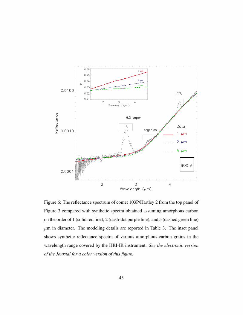
Figure 6: The reflectance spectrum of comet 103P/Hartley 2 from the top panel of

Figure 3 compared with synthetic spectra obtained assuming amorphous carbon

on the order of 1 (solid red line), 2 (dash-dot purple line), and 5 (dashed green line)

µm in diameter. The modeling details are reported in Table 3. The inset panel

shows synthetic reflectance spectra of various amorphous-carbon grains in the

wavelength range covered by the HRI-IR instrument. See the electronic version

of the Journal for a color version of this figure.

45

Figure 7: The reflectance spectrum of comet 103P/Hartley 2 from the bottom

panel of Figure 3 compared with synthetic spectra obtained assuming an areal

mixture of amorphous-carbon and water ice grains on the order of 0.82 (red), 2

(blue), 5 (purple), 10 (green), and 100 (brown) µm. The modeling details are

reported in Table 3. The inset panel shows synthetic reflectance spectra of various

sized water ice grains in the wavelength range covered by the HRI-IR instrument.

46

Figure 8: The reflectance spectrum of comet 103P/Hartley 2 from the bottom

panel of Figure 3 compared with synthetic spectra obtained assuming an areal

mixture of amorphous carbon and water ice at different phase and temperatures.

We compare models obtained with optical constants from Mastrapa et al. [2009]

of amorphous (Ia) and crystalline (Ic) water ice at 120 K (purple and yellow line,

respectively), and with optical constants of Warren and Brandt [2008] for crys-

talline ice at 266K (red line). The inset panel shows synthetic reflectance spectra

of 100% water ice (1 µm particle size) computed using the same set of optical

constants.

47

Figure 9: Models of the water ice-rich spectrum of Hartley 2 observed 7 min post-

CA assuming an intimate mixture. All sizes of water ice lead to poor solutions

when intimately mixed with dark refractory materials.

48

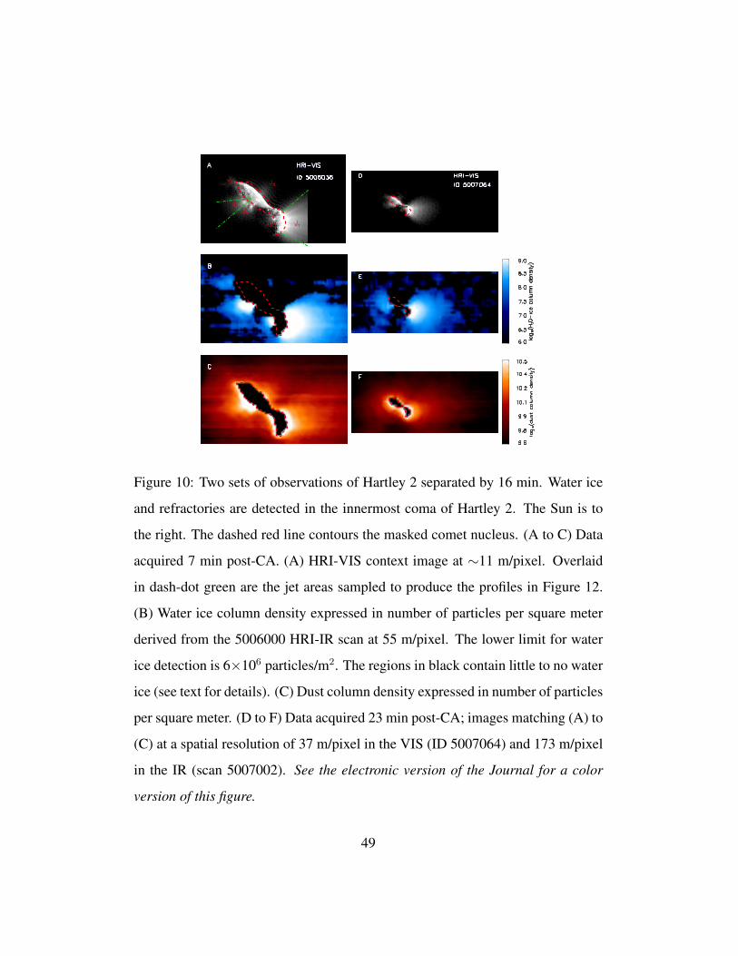
Figure 10: Two sets of observations of Hartley 2 separated by 16 min. Water ice

and refractories are detected in the innermost coma of Hartley 2. The Sun is to

the right. The dashed red line contours the masked comet nucleus. (A to C) Data

acquired 7 min post-CA. (A) HRI-VIS context image at ∼11 m/pixel. Overlaid

in dash-dot green are the jet areas sampled to produce the profiles in Figure 12.

(B) Water ice column density expressed in number of particles per square meter

derived from the 5006000 HRI-IR scan at 55 m/pixel. The lower limit for water

ice detection is 6×106 particles/m2. The regions in black contain little to no water

ice (see text for details). (C) Dust column density expressed in number of particles

per square meter. (D to F) Data acquired 23 min post-CA; images matching (A) to

(C) at a spatial resolution of 37 m/pixel in the VIS (ID 5007064) and 173 m/pixel

in the IR (scan 5007002). See the electronic version of the Journal for a color

version of this figure.

49

Figure 11: Distribution of H2O-gas, CO2, Dust, and H2O-ice in the innermost

coma of Hartley 2 as observed 7 min (left column) and 23 min (right column)

post-CA. The Sun is to the right. The dashed red line contours the masked comet

nucleus. Enhancements in the CO2 and H2O-gas relative abundances are not cor-

related. On the other hand, a strong correlation between CO2, H2O-ice, and dust

is observed in the inner coma. In all panels white is relatively more abundant. See

the electronic version of the Journal for a color version of this figure.

50

Figure 12: Column density profiles of the dust (squares) and water ice (circles) in

the jets J1 (left panel) and J4 (right panel) delimited by the dash-dot green lines

shown in panel (A) of Figure 10. Solid and dashed lines represent the models of

the dust and water ice profiles, respectively. While the dust presents a constant

outflow profile, a steeper profile is displayed by the water ice, which can be fit

by an exponential decay (see text for details). See the electronic version of the

Journal for a color version of this figure.

51