Water content – void ratio swell–shrink paths of compacted ...soilvision.com/subdomains/unsaturatedsoil.com/Docs... · The swelling potential of an expansive soil is commonly

Water content – void ratio swell–shrink paths ofcompacted expansive soils

S. Tripathy, K.S. Subba Rao, and D.G. Fredlund

Abstract: This paper addresses the behaviour of compacted expansive soils under swell–shrink cycles. Laboratory cy-clic swell–shrink tests were conducted on compacted specimens of two expansive soils at surcharge pressures of 6.25,50.00, and 100.00 kPa. The void ratio and water content of the specimens at several intermediate stages during swell-ing until the end of swelling and during shrinkage until the end of shrinkage were determined to trace the water con-tent versus void ratio paths with an increasing number of swell–shrink cycles. The test results showed that the swell–shrink path was reversible once the soil reached an equilibrium stage where the vertical deformations during swellingand shrinkage were the same. This usually occurred after about four swell–shrink cycles. The swelling and shrinkagepath of each specimen subjected to full swelling – full shrinkage cycles showed an S-shaped curve (two curvilinearportions and a linear portion). However, the swelling and shrinkage path occurred as a part of the S-shaped curve,when the specimen was subjected to full swelling – partial shrinkage cycles. More than 80% of the total volumetricchange and more than 50% of the total vertical deformation occurred in the central linear portion of the S-shapedcurve. The volumetric change was essentially parallel to the saturation line within a degree of saturation range of 50–80% for the equilibrium cycle. The primary value of the swell–shrink path is to provide information regarding the voidratio change that would occur for a given change in water content for any possible swell–shrink pattern. It is suggestedthat these swell–shrink paths can be established with a limited number of tests in the laboratory.

Key words: expansive soils, oedometer tests, swell–shrink behaviour, shrinkage tests.

Résumé : Cet article traite du comportement des sols gonflants compactés sous des cycles de gonflement-retrait. Lesessais en laboratoire de gonflement–retrait ont été réalisés sur des spécimens compactés de deux sols gonflants à despressions de surcharge de 6,25, 50,00, et 100,00 kPa. On a déterminé l’indice des vides et la teneur en eau des spéci-mens à plusieurs étapes intermédiaires durant le gonflement jusqu’à la fin du gonflement, et durant le retrait jusqu’à lafin du retrait, pour tracer le cheminement de la teneur en eau en fonction de l’indice des vides avec le nombre crois-sant de cycles de gonflement–retrait. Les résultats d’essais ont montré que le cheminement gonflement–retrait était ré-versible une fois que le sol avait atteint une étape d’équilibre où les déformations verticales durant le gonflement et leretrait étaient les mêmes. Cette étape était généralement atteinte après environ quatre cycles de gonflement–retrait. Lecheminement de gonflement et retrait de chaque spécimen assujetti à des cycles de gonflement complet et retrait com-plet ont montré une courbe en forme de « S » (deux portions curvilignes et une portion linéaire). Cependant, le chemi-nement de gonflement et retrait se produisait le long de la courbe en forme de « S » lorsque le spécimen était soumisà des cycles de gonflement–retrait partiel. Plus de 80 % du changement volumétrique total et plus de 50 % de la dé-formation verticale totale se sont produits le long de la portion centrale linéaire de la courbe en forme de « S ». On atrouvé que le changement volumétrique était essentiellement parallèle à la ligne de saturation à l’intérieur d’un degréde saturation variant dans la plage de 50 à 80 % pour le cycle d’équilibre. La valeur première du cheminement gonfle-ment–retrait est de fournir de l’information quant au changement de l’indice des vides qui se produirait pour un chan-gement donné de teneur en eau pour n’importe quel schéma possible de gonflement–retrait. On croit que cescheminements gonflement–retrait peuvent être établis avec un nombre limité d’essais en laboratoire.

Mots clés : sols expansifs, essais oedométriques, comportement gonflement–retrait, essais de retrait.

[Traduit par la Rédaction] Tripathy et al. 959

Introduction

Engineering problems related to expansive soils have beenreported in many countries of the world but are generally

most serious in arid and semiarid regions. As a result, highlyreactive soils undergo substantial volume changes associatedwith the shrinkage and swelling processes. Consequently,many engineered structures suffer sever distress and damage.

Can. Geotech. J. 39: 938–959 (2002) DOI: 10.1139/T02-022 © 2002 NRC Canada

938

Received 11 July 2001. Accepted 17 January 2002. Published on the NRC Research Press Web site at http://cgj.nrc.ca on24 July 2002.

S. Tripathy.1 School of Civil and Structural Engineering, Nanyang Technological University, Singapore 639 798, Singapore.K.S. Subba Rao. Department of Civil Engineering, Indian Institute of Science, Bangalore 560 012, India.D.G. Fredlund. Department of Civil Engineering, University of Saskatchewan, Saskatoon, SK S7N 5A9, Canada.

1Corresponding author. Present address: Marienstrasse 7, Room 110, Bauhaus University Weimar, 99421 Weimar, Germany(e-mail: [email protected]).

I:\cgj\Cgj39\Cgj-04\T02-022.vpMonday, July 22, 2002 1:57:52 PM

Color profile: DisabledComposite Default screen

The swelling potential of an expansive soil is commonlyassessed in the laboratory by utilizing a conventional oedo-meter apparatus. The specimens are generally allowed toswell under an arbitrary surcharge pressure for one cycle todetermine the total magnitude of swell.

Laboratory cyclic swell–shrink tests on expansive soilshave shown that vertical swell potential may reduce or evenincrease by a factor of two when compared with the first cy-cle of swelling. Therefore, the assessment of expansive soilbehaviour without considering cyclic seasonal fluctuationsmay underestimate the swelling potential of the soil.

A number of research studies are available on laboratorycyclic swell–shrink tests on compacted–remolded expansivesoils. The studies have shown that after about three to fiveswell–shrink cycles, the soils reach an equilibrium condi-tion, where the vertical deformations during swelling andshrinkage are the same (Warkentin and Bozozuk 1961;Popescu 1980; Subba Rao and Satyadas 1987; Day 1994;Al-Homoud et al. 1995; Songyu et al. 1998). This reversiblevolume change between fixed limits has been observed forsurface horizons of agricultural soils that have undergonenumerous drying and wetting cycles (Yong and Warkentin1975).

Ring (1966) showed that the height changes of specimensduring wetting and drying are the same after four cycles, andare even independent of the initial compaction conditions.The void ratio after each swell–shrink cycle determined forremolded soil specimens subjected to cycles of full swellingand full shrinkage, or full swelling and partial shrinkage, hasbeen reported by Basma et al. (1996). The test results indi-cate that the void ratio remains at a consistent value afterequilibrium is reached. Subba Rao et al. (2000) have shownthat for compacted clays subjected to cycles of wetting anddrying, the ultimate void ratio is independent of the initialcompaction conditions. Results of shrink–swell tests byWarkentin and Bozozuk (1961) and Dif and Bluemel (1991)have also shown that the water content of the soil specimensreaches a consistent value after about four swell–shrink cy-cles. Cyclic swell–shrink tests conducted on compacted ex-pansive soils by Tripathy (2000) agree well with the findingscited here.

The volume change of a soil in the field is in reality athree-dimensional phenomenon. Jennings and Kerrich (1962)have stated that soil heave occurs primarily normal to theground surface because lateral swelling is largely inhibitedby adjacent soil. Parcher and Liu (1965), on the other hand,have shown that undisturbed clay specimens can have signif-icant lateral swelling that may even be greater than theswelling normal to the ground surface. Gromko (1974) andYong and Warkentin (1975) have highlighted the importanceof studying the volume-change characteristics of soils inslopes and soils behind retaining-wall structures. Dependingon the situation, vertical deformation, lateral deformation, orboth types of deformation might be of dominant interest tothe designer. Volume-change measurements and vertical-deformation measurements are common in geotechnical en-gineering practice because of the absence of a specific testprocedure for lateral swelling measurements. A review ofthe literature indicates that there has been considerable inter-est in understanding the cyclic swell–shrink potential of ex-pansive soils. This has been accomplished by measuring the

vertical deformation of soils undergoing cycles of swellingand shrinkage. The change in volume of the soil, however,and the changes in water content from the shrinkage state tothe saturation state and from the saturation state to theshrinkage state have not been fully studied.

This paper presents the results of a comprehensive studyof the water content versus void ratio paths for two com-pacted expansive soils during swell–shrink cycles until theequilibrium conditions were attained. The tests extendedthrough a series of cyclic swell–shrink tests under severalsurcharge pressures. The effect of initial placement condi-tions (e.g., dry density and water content) and partial shrink-age on the swell–shrink water content – void ratio pathsunder a low surcharge pressure is also examined.

Literature review

The change in void ratio with a change in water contentfor an expansive soil as a result of desiccation and water ab-sorption provides an understanding of swelling and shrink-age behaviour (Hanafy 1991). Fredlund and Rahardjo (1993)have stated that the shrinking and swelling relationship for asoil relate the void ratio to the water content at variousmatric suctions. In situations where there is a gradual de-crease in water content upon drying, the air-entry value ofthe soil is indistinct and the shrinkage curve must be used inconjunction with the soil-water characteristic curve to deter-mine the correct air-entry value of the soil.

The assessment of soil volume change as a function ofwater content during the shrinkage of a soil has been thesubject of considerable research (Dasog et al. 1988; Ho et al.1992; Mitchell and van Genuchten 1992; Sitharam et al.1995; Marinho and Stuermer 1999). Shrinkage curves ofsoils are usually determined by drying undisturbed, com-pacted, or initially slurried soil specimens. The initiallyslurried specimens are used to determine the shrinkage limitof the soil (American Society for Testing and Materials(ASTM) test method D427, ASTM 1998c). In all the meth-ods, specimens are dried for one cycle with zero externalstress applied.

The shrinkage curve of a soil specimen shows differentphases of deformation. Haines (1923) distinguished the dif-ferent phases of shrinkage that result from progressive dry-ing of natural soils: (i) structural shrinkage, (ii) normalshrinkage, and (iii) residual shrinkage. During structuralshrinkage a few large, stable pores are emptied and the de-crease in volume of the soil is less than the volume of waterlost. During the normal shrinkage phase, volume decrease isequal to the volume of water lost (i.e., the slope of the totalspecimen volume versus water content line is 45°). On fur-ther drying, the slope of the shrinkage curve changes and airenters the voids at the shrinkage limit or at the start of resid-ual shrinkage. As the particles come in contact, the decreasein specimen volume is less than the volume of water lost.Lastly, when all the particles come close together, no furthershrinkage occurs while water is still being lost. This phasehas been identified as the no-shrinkage stage by Stirk (1954).

Different models have been proposed for describing thesoil shrinkage characteristic curve. All models use an S-shaped continuous curve with a linear normal shrinkage phase(Crescimanno and Provenazano 1999). The structural and

© 2002 NRC Canada

Tripathy et al. 939



residual phases are either flattened or sloped. Figure 1ashows a general form for the shrinkage curve consisting ofthree straight-line portions to the water content versus vol-ume plot, corresponding to the three phases of shrinkage.

Laboratory tests such as the coefficient of linear extensi-bility (COLE) test (Brasher et al. 1966) and the CLOD test(McKeen and Hamberg 1981) have been used to measure thewater content versus void ratio relationship for undisturbedsoil clods. The test procedures include measuring the vol-ume change of a soil clod during drying while simulta-neously protecting the clod from losing soil materials bycoating it with Saran resin. The CLOD test method is amodification of the COLE method in that the void ratio ver-sus water content plot is determined by periodically moni-toring the volume change and water content change duringthe drying process. In the COLE test, the void ratio and wa-ter content of a clod are measured only at a suction of 0.33atm (1 atm = 101.325 kPa) and at the driest state of the soil.The slope of the normal shrinkage curve (i.e., water contentversus void ratio curve) obtained from the CLOD test is des-ignated as the CLOD index, Cw. Typical values of Cw arefrom 0.00 to 0.17 for soils in the western and midwesternUnited States (Fredlund and Rahardjo 1993) and about 0.02for Pierre Shale (Nelson and Miller 1992).

Research studies have been conducted to study the effectof the initial volume of the clod, the initial water content ofthe clod, and Saran resin on the measured COLE values.These investigations have raised concerns regarding the sizeof the clods to be used (McIntyre and Loveday 1968), the ef-fect of the initial water content of the specimens at the timeof coating with Saran resin (Tunny 1970), and the use of Sa-ran resin (Anderson et al. 1972). Crescimanno andProvenazano (1999) reported that there is a significant dif-ference in shrinkage characteristic curves of clay soils whenmeasurements are made using small natural clods coatedwith resin and larger soil specimens. Less shrinkage was ob-served in the case of larger specimens compared with theshrinkage of the clods.

Nelson and Miller (1992) commented that the CLODmethod does not consider the stress state and hence is appli-cable only for the determination of free field heave underlight loads such as pavements or floating floor slabs. In anycase, the CLOD tests measurements cannot be viewed as arigorous measurement of volume change versus water con-tent change for practical engineering problems.

Ho et al. (1992) conducted shrinkage tests on compactedglacial till and compacted silt specimens. The test resultsshowed that the shrinkage test curve moves away from thesaturation line as the initial water content is lowered.

Shrinkage tests on compacted soils have provided infor-mation on both volumetric and axial shrinkage (Kezdi 1980;Sitharam et al. 1995). Subba Rao and Satyadas (1985) con-ducted shrinkage tests on compacted specimens and reporteda curvilinear relationship between volumetric and linearshrinkage. Padmanabha (1988) has shown that for com-pacted soils, the linear shrinkage generally lies within onequarter to one sixth of the volumetric shrinkage for initialand later parts of shrinkage, but the specific ranges are notwell defined.

Erol (1992) conducted field and laboratory swelling testsand reported that the ratio of volumetric to linear strain was

about three. Crilly et al. (1992) showed that the ratio ofvertical to volumetric strain is not constant throughout aswelling layer, hence the use of a single factor would tend tooverestimate movements near the ground surface and under-estimate movements at depth.

Similar to the multiphase shrinkage behaviour of a soilspecimen, the swelling of desiccated soils also occurs inthree different phases (Day 1999), namely primary swelling,secondary swelling, and no swelling. During primary swell-ing, the cracks developed during drying close. Primaryswelling occurs at a very rapid rate. Secondary swelling in-cludes closure of microcracks and reduction of entrapped air.During the third phase (i.e., no swelling), no further void ra-tio changes occur. The three phases of swelling of desiccatedOtay Mesa clay from Day (1999) are shown in Fig. 1b.

Hanafy (1991) proposed a characteristic S-shaped curve todescribe the potential volume change of an expansive clayeysoil for the change in void ratio relative to changes in watercontent resulting from desiccation and water absorption. TheS-shaped curve (Fig. 2) can be determined in the laboratoryusing conventional consolidation test equipment by carryingout one complete swelling–shrinkage test with two addi-tional partial tests. Expansive soil specimens, desiccated orpartially desiccated with an initial water content, wn, and acorresponding natural void ratio, e0, are used to trace thepath during testing. The S-shaped curve can be used to clas-sify the swelling potential of desiccated expansive clayeysoils.

Swell–shrink paths are usually shown as a water contentversus matric suction plot or as a water content versus voidratio plot. The drying and wetting tests are conducted in apressure-plate apparatus such as the volumetric pressure plateextractor to determine water contents corresponding to vari-ous matric suctions as the specimen is dried and rewetted. Ithas been observed that hysteresis causes the constitutive sur-faces obtained from drying to be different from the surfacesobtained from wetting (Croney and Coleman 1954; Fleureauet al. 1993; Fredlund and Rahardjo 1993).

The hysteresis in the wetting–drying path indicates that, atany given matric suction, the water content during drying ofa specimen is greater than the water content during wettingof the specimen. Similarly, at the same water content, thematric suction during drying is larger than the matric suctionduring wetting. The hysteresis phenomenon has been ex-plained in terms of the so-called “ink-bottle effect” (Yongand Warkentin 1975). The ink-bottle effect considers theamount of void space in a granular soil comprised of differ-ent grain sizes during wetting and drying for describing thehysteresis phenomenon. In the case of clayey soil, however,particle rearrangement during shrinkage and swelling andchanges in water content complicate the understanding ofthe hysteresis phenomenon. It is not fully understood whetherthe water content alone or the water content and void ratiotogether are responsible for hysteresis along the wetting–drying path of a clayey soil.

Mitchell (1976) and Chen (1988) have pointed out that,although swelling and shrinking of expansive clays are inter-related, it is uncertain whether highly swelling clays alsoshow equally high shrinkage upon drying. Songyu et al.(1998) stated that since height changes of specimens in-crease with shrink–swell cycles, the swelling–shrinkage

© 2002 NRC Canada

940 Can. Geotech. J. Vol. 39, 2002



behaviour of an expansive soil is not completely reversible.On the other hand, Haines (1923) observed that if the soildrying does not extend below the shrinkage limit, then wet-ting and drying take place in a reversible manner. Yong andWarkentin (1975) have also stated that clayey soils contain-ing montmorillonite show almost reversible swelling andshrinkage on rewetting and redrying.

Numerous researchers have studied the wetting and dryingpaths in terms of water content and soil suction. Studies onthe water content – void ratio path with swell–shrink cyclesare limited; however, some studies (e.g., Haines 1923) havebeen conducted on undisturbed unconfined specimens fortwo swell–shrink cycles. The effect of surcharge pressure,initial placement condition (viz., dry density and water con-tent), and swell–shrink pattern (e.g., full swelling – full

shrinkage and full swelling – partial shrinkage) on the watercontent – void ratio path for compacted expansive soils withswell–shrink cycles has not been fully studied. Studies onthe swell–shrink behaviour of expansive soils tested in oedo-meters suggest that the vertical deformation, void ratio, andwater content after about four swell–shrink cycles are re-versible (Subba Rao 2000). It is not known if the paths dur-ing wetting and drying, in terms of water content and voidratio, are reversible at equilibrium. The intent of this paperis to experimentally study the effect of surcharge pressure,initial placement conditions, swell–shrink pattern, and num-ber of swell–shrink cycles on the water content – void ratioswelling and shrinkage paths of compacted expansive soils.

Theory of swell–shrink

The volume–mass relationships between soil solids, water,and air phases are useful properties in engineering practice(Fredlund and Rahardjo 1993). The volume–mass relation-ships can be represented as a three-phase diagram as shownin Fig. 3a. With reference to the three-phase diagram, thewater content, w, void ratio, e, and degree of saturation, Sr,are defined in Fig. 3a as eqs. [1], [2], and [3], respectively.The relationship between eqs. [1], [2], and [3] is known asthe basic volume–mass relationship for soils (eq. [4] inFig. 3a). The basic volume–mass relationship applies to anycombination of Sr, e, and w. A change in any one of thesevolume–mass properties (i.e., Sr, e, and w) may producechanges in the other two properties.

The total volume measurement of a dried specimen ofknown mass can be performed in two ways: (i) by measuringthe dimensions of the specimen using calipers, and (ii) bythe mercury displacement technique (ASTM test methodD427, ASTM 1998c). Shrinkage of the soil specimens in-variably leads to a reduction in cross-sectional area accom-panied by the development of shrinkage cracks, particularlyif the specimens are dried at an elevated temperature (Subba

© 2002 NRC Canada

Tripathy et al. 941

Fig. 1. Different phases of (a) shrinkage and (b) swelling. e0,initial void ratio; Hi, initial height of the specimen.

Fig. 2. Illustration of the S-shaped curve (water content – voidratio relationship).



Rao et al. 2000). In such cases, determination of the volumeof the specimen by the mercury displacement technique hasbeen proven to be more accurate. By knowing the mass ofthe dry specimen, Ms, and volume of the dry specimen, V,from the mercury displacement technique, the dry density,ρd, can be determined from eq. [6] in Fig. 3a. The volumemeasurement of specimens that are partially dried can alsobe performed using the mercury displacement technique(Hanafy 1991; Subba Rao et al. 2000). In such cases, the dry

density can be determined from eq. [7] in Fig. 3a by know-ing the total density (eq. [5], Fig. 3a) and water content ofthe specimen. The water content of the specimen can be in-dependently measured by oven-drying the specimen. Thevoid ratio, e, is determined from the relationship betweendry density and void ratio as given by eq. [8] in Fig. 3a.

The volume of voids is the summation of the volume ofthe water phase and the volume of the air phase (i.e., Vv =Vw + Va). In the case of an unsaturated soil, the volume of

© 2002 NRC Canada


Fig. 3. (a) Three-phase diagram of unsaturated soil. Gs, specific gravity; ρ, density; ρd, dry density. (b) Phase diagram during swellingand shrinkage.



voids, Vv, is the variable, since the volume of soil solids isconstant (i.e., assuming the soil particles to be incompress-ible). Figure 3b shows the phase diagrams associated withswelling and shrinkage volume changes in soils. The volumechange is expressed as the change in volume of voids asgiven by eq. [9] in Fig. 3b.

Volume change is usually determined in the one-dimensional oedometer swelling test by recording thechange in height of the specimen. The volume change can becomputed using eq. [10] in Fig. 3b. In oedometer swell–shrink tests, the specimens shrink and swell three-dimensionally, except in the first swelling cycle (i.e., swell-ing from the as-compacted state). At the end of all swellingcycles, the diameter of the specimen is equal to the diameterof the oedometer ring, but the height changes during eachswelling cycles may be different. The diameter of a fullydried specimen is usually less than the diameter of the oedo-meter ring. Since the lateral dimensional changes of thespecimen during each swelling and shrinkage cycle are notmanifested by the height changes, eq. [10] cannot be used todetermine the volume change. Considering the void ratiochange during swelling and shrinkage as ∆e, the volumechange can be written as given by eq. [11] in Fig. 3b.

Soils used and testing procedures

Two expansive soils collected from the NorthernKarnataka State of India were selected for the study. Thenatural soils were processed to be finer than 425 µm with re-sulting liquid limits of 100 and 74%. These soils are calledsoils A and B, respectively. The properties of the soils arepresented in Table 1. Laboratory test procedures, followingASTM standards, were performed to evaluate the physicalproperties of the soils. The free swell properties of the soilswere determined as per the procedure given by Holtz andGibbs (1956). Figure 4 shows the standard Proctor (ASTMtest method D698, ASTM 1998b) and modified Proctor(ASTM test method D1557, ASTM 1998a) compactioncurves for the soils. The shrinkage limit and liquid limit ofthe soils indicate that both soils are highly plastic and havehigh moisture absorption capacities. X-ray diffraction patternsof magnesium-saturated and glycerol-solvated specimens ofsoils A and B show the existence of montmorillonite as thedominating clay mineral (Fig. 5). The Indian standard classi-fication system (IS 1498, Bureau of Indian Standards 1970)classifies the “degree of expansion” and “danger of severity”

of both the soils as very high and severe, respectively. Theclassification is based on the liquid limit (wl), plasticity in-dex (Ip = wl – wp), and shrinkage index (Is = wl – ws) values,where wp is the plastic limit of the soil, and ws is the shrink-age limit of the soil.

The specimen conditions selected for the study are markedon the compaction curves for both soils (Fig. 4). Specimenswere selected such that the dry density could be varied whilethe water content remained constant (specimens A1 and A11for soil A, and specimens B1 and B11 for soil B) and thedry density was maintained constant while the water contentwas varied (specimens A1 and A6 for soil A, and specimensB1 and B6 for soil B). In addition, specimens A3 for soil Aand B3 for soil B were chosen to represent the standardProctor optimum conditions of the respective soils. Severalmixes were prepared using the air-dried soil mixed with pre-determined quantities of water. The mixes were kept inclosed plastic bags and cured for 7 days. After ensuring thedesired water content for the mix, the moist soil was com-pacted to a height of 13 ± 0.5 mm directly into a stainlesssteel oedometer ring, 76.2 mm in diameter and 38 mm inheight. Laboratory static compaction was used to achieve thedesired dry densities.

Cyclic swell–shrink tests

Cyclic swell–shrink tests were conducted in a fixed-ringoedometer with a modification to shrink the specimens un-der a controlled surcharge pressure and temperature (i.e.,40 ± 5°C). A schematic diagram of the setup is shown inFig. 6. The setup consists of a fixed-ring oedometer cellplaced inside a stainless steel container (outer jacket). Theouter face of the outer jacket holds a 1 kW capacity coiltightly sandwiched between two flexible asbestos sheets.The flexible asbestos sheets serve as an insulator. The twoends of the coil were connected to porcelain connectors towhich power was provided through a temperature controller.A known surcharge pressure was applied to each specimenby means of the lever arm of action of the oedometer frame.The specimens were then allowed to swell after being inun-dated with water under an ambient temperature. After com-pletion of the full swelling process, the process of shrinkagewas commenced. To start the shrinkage process, water wasremoved from the inner cell (i.e., water jacket) and then thetemperature controller was switched on to maintain a con-stant temperature throughout the shrinkage process.

Proper precaution was taken while attending the oedo-meter cells by wearing a medical mask to avoid health haz-ards from the asbestos insulators. Similarly, a pair of gloveswas used while dealing with the electrical connections toavoid fatal shock.

Observation of vertical movements of the specimens dur-ing swelling and shrinkage were made by using a dial gaugewith a minimum reading of ±0.002 mm and a travel of25 mm. The combination of one swelling and shrinkage cy-cle is designated as one swell–shrink cycle. At the end ofeach cycle, the temperature controller was switched off andthe specimen temperature was returned to room temperaturein about 2–3 h. The specimen was again inundated with wa-ter for the next swelling and then shrinkage process to com-plete the second cycle. Thus, several cycles of swelling and

© 2002 NRC Canada

Tripathy et al. 943

Soil A Soil B

Liquid limit, wl (%) 100 74Plastic limit, wp (%) 42 32

Plasticity index, Ip (%) 58 42

Shrinkage limit, ws (%) 10.6 13.5

Specific gravity, Gs 2.68 2.73

% passing sieve No. 200 (425 µm) 98 80

Clay content (<0.002 mm; %) 62 52

Silt content (%) 36 28

Fine sand content (%) 2 20

Free swell (%) 340 225

Table 1. Properties of the soils used in the study.



shrinkage were performed until the specimen reached equi-librium conditions. Equilibrium was defined as the conditionwhere swelling and shrinkage were of constant magnitudefor each cycle. In the case of full swelling followed by fullshrinkage tests, specimens in each cycle were allowed tofully swell and then shrink to a stage where there was nofurther change in height. The time allowed for each swellingprocess was about 3 days, and the full shrinkage process re-quired about 6 days to complete at a temperature of 40°C. Inthe case of full swelling followed by partial shrinkage, spec-imens in each cycle were allowed to fully swell and thenshrink to a height corresponding to 50% of the first swollenheight in each cycle. The time taken for partial shrinkagewas about 2 days.

The vertical deformation of the specimens was repre-sented as the change in height (∆H) of the specimen (duringeither swelling or shrinkage) and is expressed as a percent-age of the initial height of the specimen (Hi) at the begin-ning of the first swell–shrink process. By plotting thevertical deformations of a specimen for several swell–shrinkcycles, the percent change in height of the specimen duringany of the swelling or shrinkage cycles can be observed.

Swell–shrink paths

The height of the specimen and the water content of thespecimen subjected to swell–shrink cycles under a given sur-charge pressure, at the end of each swelling and shrinkagecycle, were first determined. A number of duplicate speci-mens were prepared corresponding to the same initial place-ment conditions as those for the first specimen. These

specimens were subjected to cyclic swell–shrink tests underthe same surcharge pressure. The initial water content anddry density of the duplicate specimens were within a permis-sible error of about ±0.5%. To trace the swelling path of thespecimen within each cycle, at least five or six specimenswere tested. Once the previous shrinkage cycle was endedfor these specimens, water was supplied with the help of amedical syringe to each of the specimens through the ventsprovided in the pressure pad (Fig. 6). The intention was notto allow the specimens to swell fully. The quantity of watersupplied to each specimen was decided by trial and error.The tests were terminated when the height changes of thespecimens became insignificant. Similar procedures wereadopted for each cycle until equilibrium conditions were at-tained. Similarly, to trace the shrinkage path of the specimenwithin each cycle, at least five or six specimens were tested.The height at which the specimens would be dismantled dur-ing each shrinkage cycle was arbitrarily fixed at one sixth,one third, two thirds, and five sixths of the total heightchange in that cycle. The number of specimens tested was in-creased as necessary to bring clarity to the swell–shrink paths.Fewer specimens were required to trace the swell–shrink pathunder higher surcharge pressures and the full swelling – par-tial shrinkage test. Table 2 shows the number of specimensused to trace the swell–shrink path under each surchargepressure for soils A and B.

Shrinkage of soil specimens invariably leads to a reduc-tion in cross-sectional area accompanied by the developmentof shrinkage cracks. At intermediate stages, before fullswelling, cracks were still present in the specimen. The vol-ume of the specimens at intermediate stages before the end

© 2002 NRC Canada


Fig. 4. Standard Proctor and modified Proctor curves for soils A and B used in the test program.



© 2002 NRC Canada

Tripathy et al. 945

Fig. 5. X-ray diffraction patterns of the soils used in the test program (after Tripathy 2000).

Fig. 6. Schematic diagram of the experimental setup. 1, outer stainless steel jacket; 2, water jacket; 3, bottom porous stone; 4, outerring; 5, specimen ring; 6, pressure pad; 7, pressure ball; 8, top porous stone.



of swelling, and at different stages of shrinkage in the subse-quent cycles after the first swelling cycle, was determinedusing the mercury displacement technique. Extreme care wasexercised while handling mercury by wearing gloves and amedical mask. The precautions to be taken during handlingmercury are suggested in ASTM test method D427 (ASTM1998c). In the first swelling cycle, the height of the speci-men was used as a reference for calculating the volume ofthe specimen. Each time a specimen was dismantled, itsmass was immediately measured and then its volume wasmeasured. The water content was determined by oven-drying.Knowing the total density (from the mercury displacementtechnique) and water content, the dry density was calculatedusing eq. [6] in Fig. 3a. Using eq. [7] in Fig. 3a, the void ra-tio of each specimen was determined.

The surcharge pressures applied to the specimens were6.25, 50.00, and 100.00 kPa for specimen A3 of soil A and6.25 and 50.00 kPa for specimen B3 of soil B (see Table 2).The effect of initial placement conditions on the equilibriumswell–shrink path was studied under a surcharge pressure of6.25 kPa. The effect of full swelling – partial shrinkage wasstudied for specimen A3 of soil A under a surcharge pres-sure of 6.25 kPa.

Presentation of test results

Vertical deformationsThe effect of surcharge pressure on the vertical deforma-

tions for specimens A3 and B3 with swell–shrink cycles ispresented in Figs. 7a and 7b, respectively. The vertical de-formation upon the first cycle of swelling decreased with anincrease in surcharge pressure. Under all surcharge pres-sures, the vertical deformations of the specimens during thefourth swelling cycle and fourth shrinkage cycle were greaterthan the corresponding vertical deformation during the firstcycle. In all cases, the deformation due to swelling andshrinkage was the same after about four or five swell–shrinkcycles, indicating that an equilibrium state had been reached.The vertical deformation at the equilibrium state was 20.39,14.34, and 10.37% for specimen A3 under surcharge pres-sures of 6.25, 50.00, and 100.00 kPa, respectively. The de-formation at the equilibrium state for specimen B3 was14.47 and 10.36% under surcharge pressures of 6.25 and50.00 kPa, respectively.

The effect of initial placement conditions on the swell–shrink behaviour of soils A and B is shown in Figs. 8a and

8b, respectively. The initial placement conditions are alsoshown in the figures. The vertical deformation for the firstcycle of swell–shrink was somewhat different for the speci-mens of the same soil. At the same initial water content theamount of swell increased with an increase in dry density.On the other hand, at the same dry density the amount ofswell decreased with an increase in water content. These ob-servations are similar to the trends reported by Holtz andGibbs (1956) for compacted expansive soils. Interestingly,irrespective of the initial conditions of the specimens, thevertical deformation after about the third cycle of swell–shrink was nearly the same for all specimens tested of eachsoil. This indicates that the initial placement conditions areof secondary influence after several swell–shrink cycles. Thevertical deformation at the equilibrium state is about 20.5%for specimens of soil A and 14.5% for specimens of soil B.Specimens A3 and B3 also showed about the same verticaldeformation at the equilibrium state as shown in Figs. 7aand 7b, tested with a surcharge pressure of 6.25 kPa.

Figure 9 shows the effect of full swelling and partialshrinkage cycles on specimen A3 under a surcharge pressureof 6.25 kPa. The vertical deformation for each cycle of swell–shrink was less than the deformation of the same specimensubjected to the full swelling – full shrinkage cycle at thesame surcharge pressure (Fig. 7a). The movement once againstabilized after about four cycles, showing a vertical defor-mation of 14%.

Water content – void ratio pathsThe void ratio changes for changes in water content in

specimen A3 under surcharge pressures of 6.25 and 50.00 kPaand specimen B3 under a surcharge pressure of 6.25 kPafrom the as-compacted state to the fourth cycle are shown inFigs. 10, 11, and 12, respectively, for swelling and shrink-age. Test results for specimen B3 under a surcharge pressureof 50.00 kPa and A3 under a surcharge pressure of 100.00 kPaexhibited similar trends.

In Fig. 10, points 0, 1, 2, 3, and 4 represent the positionsof specimens at full shrinkage stages in different cycles, andpoints B, C, D, and E represent the positions of the speci-men at full swelling for different cycles. These points arealso shown in Fig. 7. The initial void ratio and water contentof the specimens are e0 and wo (i.e., point A). The sequenceof wetting and drying of specimen A3 in Fig. 10 is as fol-lows: (i) swelling took place from point A to point B andshrinkage from point B to point 1 (Fig. 10a), (ii) swellingtook place from point 1 to point C and shrinkage from pointC to point 2 (Fig. 10b), (iii) swelling took place from point 2to point D and shrinkage from point D to point 3 (Fig. 10c),and (iv) swelling took place from point 3 to point E andshrinkage from point E to point 4. Point 4 ends up the sameas point 3 as shown in Fig. 10d. The shrinkage curve of thespecimen from position A was also traced (i.e., A to 0 inFig. 10a). Similar explanations hold for Figs. 11 and 12. InFig. 12, the specimen showed compression from A to A′ af-ter being loaded. The swell–shrink cycle in this case startedfrom A′.

Figures 10–12 show that, subsequent to swelling, all spec-imens attained almost full saturation. All swelling curves,except curve AB (i.e., specimen subjected to swelling afterapplication of surcharge pressure), and all shrinkage curves,

© 2002 NRC Canada


Surchargepressure (kPa) Type of test

No. ofspecimens

Soil A6.25 Full swelling – full shrinkage 92*6.25 Full swelling – partial shrinkage 3250.00 Full swelling – full shrinkage 45100.00 Full swelling – full shrinkage 45Soil B6.25 Full swelling – full shrinkage 62*50.00 Full swelling – full shrinkage 40

*Includes specimens from all the initial placement conditions.

Table 2. Testing program.



except curve A0 (i.e., specimen shrunk from point A (A′ inFig. 12)), are S-shaped. This indicates that the paths fromthe end of the shrinkage to the end of the swelling and fromthe end of the swelling to the end of the shrinkage consist oftwo curvilinear portions and a linear portion. It can also beseen that for a change in water content, the void ratiochanges are insignificant at the top and bottom curvilinearportions of the S-shaped curves. Except for the secondswelling path (i.e., curve 1C), the linear portions of all otherswelling and shrinkage paths are essentially parallel to the100% saturation line. The slope of the linear portion of thesecond swelling curve is slightly steeper. This indicates thata large volume change occurred in the second swelling cycleas compared with any other swelling cycle.

The shrinkage paths shifted away from the saturation lineand the specimens became more unsaturated with minimal

changes in void ratio for a decrease in water content. Thistendency essentially ends at a water content correspondingto a degree of saturation, Sr, of 80% in cycles 3 and 4. Inearlier cycles, the transition from full saturation to unsatu-rated conditions occurred at still higher degrees of satura-tion, indicating that the distance from the shrinkage curve tothe saturation line increased with an increase in the numberof swell–shrink cycles. Subsequently, the shrinkage curvestook on a slope of about 45° until the specimen approachedthe shrinkage limit water content (i.e., ws = 10.6% for soil Aand ws = 13.5% for soil B). Similar trends can be seen inFigs. 11 and 12.

The three phases of shrinkage can be identified in the en-tire shrinkage curves (i.e., structural shrinkage, normalshrinkage, and residual shrinkage). Similarly, in all theswelling curves traced from the full shrinkage stage, the

© 2002 NRC Canada

Tripathy et al. 947

Fig. 7. Vertical deformation with swell–shrink cycles: (a) soil A, and (b) soil B.



phases can be identified as primary, secondary, and noswelling. The shrinkage curves obtained by drying the speci-men from position A (A′ in Fig. 12) showed only the normaland residual shrinkage phases. The trends are similar to thoseobserved by Ho et al. (1992) and Sitharam et al. (1995)for compacted specimens subjected to one cycle of shrinkage.

The void ratios and water contents attained by the speci-mens were at a minimum at the end of the first shrinkage cy-cle. At the end of other cycles, however, higher void ratioand water content were observed. Similarly, the void ratioand water content attained by the specimen at the end of thefirst swelling cycle were lower than the corresponding val-ues at all other swelling cycles. The water content and voidratio at the end of the second swelling cycle were higher

than at any other cycle. Beyond the second cycle, the watercontent and void ratio decreased slightly and then stabilized.

Hysteresis in swelling and shrinkage paths was observedfor the first three cycles. When each specimen was allowedto shrink, the void ratio at the end of the cycle changed.Similarly, the void ratio and water content of the specimen atthe end of the swelling cycle changed when the specimenwas rewetted. This occurred until about the third cycle. Inthe fourth swell–shrink cycle, the path traced by the speci-men during both swelling and shrinkage was found to be thesame, signifying reversibility in the swelling and shrinkagepaths and the elimination of hysteresis.

The results indicate that hysteresis in the wetting–dryingpath of the soil-water characteristic curves (i.e., matric

© 2002 NRC Canada


Fig. 8. Effects of initial placement conditions on swell–shrink behaviour: (a) soil A, and (b) soil B.



suction versus water content curves) of clayey soils is due tochanges in both void ratio and water content during the ini-tial cycles but is due to changes in water content alone withan increasing number of cycles.

Effect of initial placement conditionsSpecimens A1, A6, and A11 for soil A and B1, B6, and

B11 for soil B were subjected to swell–shrink cycles under asurcharge pressure of 6.25 kPa. The water content and voidratio of specimens A1, A3, A6, and A11 for soil A and B1,B3, B6, and B11 for soil B at the end of the fourth swellingand fourth shrinkage cycles are shown in Table 3. The valuesare nearly the same for all the specimens at the respectivefull swelling and full shrinkage states.

Furthermore, a few of the specimens corresponding toplacement conditions A1, A3, A6, and A11 for soil A andB1, B3, B6, and B11 for soil B were run for five swell–shrink cycles under a surcharge pressure of 6.25 kPa. Thewater content versus void ratio paths during swelling andshrinkage were traced. An S-shaped curve was establishedfor all the specimens of each soil as shown in Figs. 13(curve XYX1) and 14 (curve X′ Y′ X1′ ). The range of voidratio and water content over which the swell–shrink path oc-curred remained almost the same as that observed for speci-mens A3 and B3 in the fourth swell–shrink cycle (Figs. 10d,11d).

The range of water content and void ratio over which theswelling and shrinkage occurred is less for soil B. This canbe attributed to the lower liquid limit of soil B. The watercontent variation in the fifth cycle was from 6.5 to 63.0% forsoil A and 6.5 to 47.0% for soil B.

Effect of surcharge pressuresFigures 13 and 14 show the equilibrium swell–shrink

paths traced at the fifth swell–shrink cycle for specimen A3under surcharge pressures of 50.00 kPa (curve MNM1) and100.00 kPa (curve PQP1) and for specimen B3 under a sur-charge pressure of 50.00 kPa (M′ N′ M1′ ). All the equilib-rium swell–shrink curves have a similar S shape. However,the range of water content and void ratio change over which

the curves occurred becomes less with an increase in sur-charge pressure.

It is evident from the results that the central straight-lineportions of all the equilibrium swell–shrink curves are withinthe degree of saturation range from about 50 to 80% and arealmost parallel to the 100% saturation line. As the surchargepressure increases, the curves are shifted towards the 100%saturation line. The equilibrium swell–shrink curves are alsosimilar to the characteristic volume change S-shaped curveproposed by Hanafy (1991), as shown in Fig. 2.

The ratio of the change in void ratio to the change in wa-ter content (i.e., ∆e/∆w) in the range of degrees of saturationfrom 50 to 80% is about 0.025 for soil A and about 0.020for soil B. This is true for all equilibrium swell–shrink pathsstudied. Although these ratios are not strictly comparablewith CLOD index values, the values are of similar magni-tude.

The plastic limit, wp, and shrinkage limit, ws, of the soilsare also indicated in Figs. 13 and 14. It can be noted that wpand ws, which have a specific meaning for an initially slurriedsoil subjected to shrinkage, have no specific meaning for thevolume change of a compacted expansive soil. The watercontents at the end of all the swelling cycles were well be-low the liquid limit of the soils and fall below or above theplastic limit of the soils.

Effect of partial shrinkageFigure 15 shows the path traced by specimen A3 from the

as-compacted state to the fourth swell–shrink cycle under asurcharge pressure of 6.25 kPa. The shrinkage in each cyclewas truncated at a predetermined height before full shrink-age (Fig. 9). In this case, the swelling and shrinkage pathsshifted towards the 100% saturation line with an increase inthe number of cycles. As the number of cycles increased, thewater content at the end of a shrinkage cycle increased,whereas it decreased at the end of a swelling cycle. Theswell–shrink path was found to be reversible after the thirdcycle. In Fig. 13, the path RSR1 represents equilibriumconditions after the fifth cycle of the full swelling – partialshrinkage path for specimen A3. Unlike the full swelling –full shrinkage path, which has an S-shaped curve, the

© 2002 NRC Canada

Tripathy et al. 949

Fig. 9. Full swelling – partial shrinkage test results for specimen A3.



© 2002 NRC Canada


Fig. 10. Water content – void ratio swell–shrink paths of specimen A3 at 6.25 kPa for full swelling – full shrinkage cycles: (a) cycle1, (b) cycle 2, (c) cycle 3, and (d) cycle 4.



© 2002 NRC Canada

Tripathy et al. 951

Fig. 11. Water content – void ratio swell–shrink paths of specimen B3 at 6.25 kPa for full swelling – full shrinkage cycles: (a) cycle1, (b) cycle 2, (c) cycle 3, and (d) cycle 4.



© 2002 NRC Canada


Fig. 12. Water content – void ratio swell–shrink paths of specimen A3 at 50.00 kPa for full swelling – full shrinkage cycles: (a) cycle1, (b) cycle 2, (c) cycle 3, and (d) cycle 4.



equilibrium curve for the full swelling – partial shrinkagecurve has only two portions, namely a curved portion nearthe full-saturation stage and a linear portion. A part of thenormal phase and the complete residual phase are absent.

The linear portion was almost parallel to the 100% saturationline. However, it does not fall within the degree of saturationrange of 50–80%, as in the case of the full swelling – fullshrinkage paths. The curve is to the right of the full

© 2002 NRC Canada

Tripathy et al. 953

Water content, w (%) Void ratio, e

Specimen InitialFourthshrinkage

Fourthswelling Initial

Fourthshrinkage

Fourthswelling

A1 26.0 6.2 63.20 1.2058 0.6242 1.727A3 35.0 6.5 63.00 1.1186 0.6242 1.733A6 41.0 6.8 62.90 1.2058 0.6240 1.735A11 26.0 7.3 63.30 0.8023 0.6236 1.742B1 21.0 6.5 46.20 1.0040 0.5918 1.289B3 30.0 6.5 46.50 0.9362 0.5826 1.295B6 34.5 6.3 46.65 1.0040 0.5937 1.293B11 21.0 6.8 46.35 0.6012 0.6012 1.288

Table 3. Water content and void ratio of the specimens at the fourth swell–shrink cycle.

Fig. 13. Equilibrium swell–shrink paths for soil A.



swelling – full shrinkage equilibrium curve and is closer tothe 100% saturation line, indicating that the specimen hadhigher water contents during swelling and shrinkage.

The results also indicate that soil swelling and shrinkageare reversible in the case of fixed swell–shrink pattern tests.The path becomes different for the same soil under the samesurcharge pressure, when the shrinkage pattern changes fromfull to partial shrinkage or partial to full shrinkage.

Volumetric change and vertical deformation atequilibrium cycle

The volumetric change during the fifth swell–shrink cyclewas calculated from eq. [10] in Fig. 3b. Similarly, the verti-cal deformations were calculated from the ratio of thechange in height to the height of the specimen at the end ofthe equilibrium shrinkage cycle (i.e., fourth shrinkage cycle).The degree of saturation at equilibrium was calculated fromeq. [4] in Fig. 3a.

The volumetric change and vertical deformation forchanges in degree of saturation during equilibrium swell–shrink cycles for the full swelling – full shrinkage tests forboth soils are shown in Fig. 16. These plots also show threedistinct phases. The plots indicate that at any degree of satu-ration, as the surcharge pressure increases, the volumetricand vertical deformation decrease. Similarly, at any defor-mation, the degree of saturation increases for the specimenswith a higher surcharge pressure.

An attempt was made to distinguish the three phases andfind the percentage of the changes (i.e., both volumetric andvertical) that occurred in each phase. The first phase ofswelling or the last phase of shrinkage is designated asphase I (Sr < 50%), the last phase of swelling or first phaseof shrinkage as phase III (Sr > 80%), and the middle phaseas phase II (Sr = 50–80%).

Table 4 shows the changes that occurred in each phase forboth soils. About 80–90% of the total volumetric change forsoil A and about 70–85% of the total volumetric change for

© 2002 NRC Canada


Fig. 14. Equilibrium swell–shrink paths for soil B.



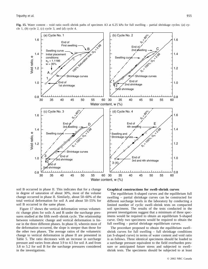
soil B occurred in phase II. This indicates that for a changein degree of saturation of about 30%, most of the volumechange occurred in phase II. Similarly, about 50–60% of thetotal vertical deformation for soil A and about 50–55% forsoil B occurred in the same phase.

Figure 17 shows the vertical deformation versus volumet-ric change plots for soils A and B under the surcharge pres-sures studied at the fifth swell–shrink cycle. The relationshipbetween volumetric change and vertical deformation is lin-ear in the three different phases. In phase II, wherein most ofthe deformation occurred, the slope is steeper than those forthe other two phases. The average ratios of the volumetricchange to vertical deformation in phase II are presented inTable 5. The ratio decreases with an increase in surchargepressure and varies from about 3.9 to 4.5 for soil A and from3.8 to 5.2 for soil B for the surcharge pressures consideredin the investigations.

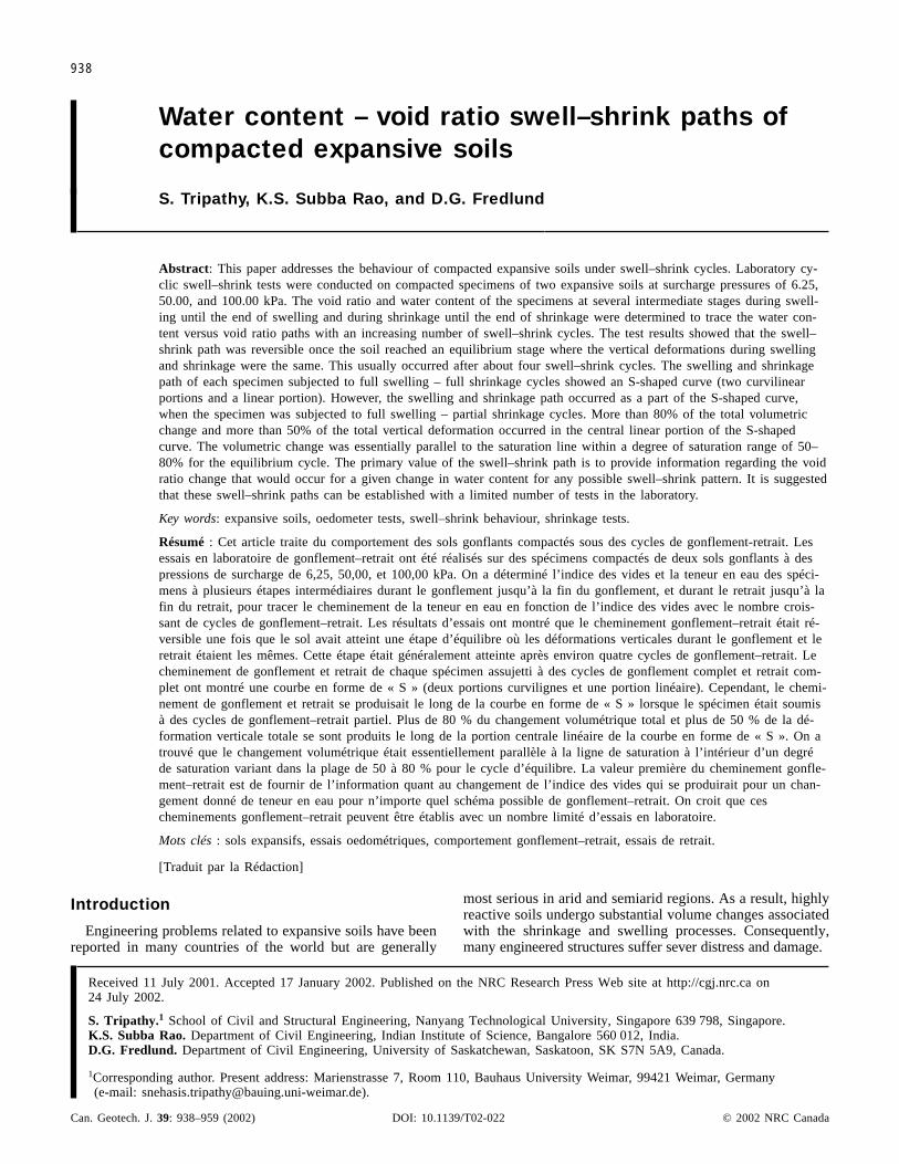
Graphical constructions for swell–shrink curvesThe equilibrium S-shaped curves and the equilibrium full

swelling – partial shrinkage curves can be constructed fordifferent surcharge levels in the laboratory by conducting alimited number of cyclic swell–shrink tests on compactedsoil specimens. The results of the tests conducted in thepresent investigations suggest that a minimum of three spec-imens would be required to obtain an equilibrium S-shapedcurve. Only two specimens would be required to obtain thefull swelling – partial shrinkage equilibrium curves.

The procedure proposed to obtain the equilibrium swell–shrink curves for full swelling – full shrinkage conditions(an S-shaped curve) in terms of water content and void ratiois as follows. Three identical specimens should be loaded toa surcharge pressure equivalent to the field overburden pres-sure or anticipated future stress and subjected to swell–shrink tests. The specimens should be subjected to at least

© 2002 NRC Canada

Tripathy et al. 955

Fig. 15. Water content – void ratio swell–shrink paths of specimen A3 at 6.25 kPa for full swelling – partial shrinkage cycles: (a) cy-cle 1, (b) cycle 2, (c) cycle 3, and (d) cycle 4.



four swell–shrink cycles. One specimen should be disman-tled at the end of the fourth swelling cycle, one at the end ofthe fourth shrinkage cycle, and the last specimen at an inter-mediate level. The intermediate point should be chosenwithin a degree of saturation range of 50–80%. The watercontent and void ratio of the three specimens should be mea-sured. On a water content versus void ratio plot, mark thethree points. The results are designated as points Y, X, and Sin Fig. 18. Draw the 100% saturation line, knowing the spe-cific gravity of the soil. Draw lines parallel to the x axisthrough points X and Y. Draw a line parallel to the satura-tion line through point S (the intermediate point) to intersectthe parallel lines at points a and b. Measure the distance Xaand mark ac equal to Xa on line ab. Measure the distanceYb and mark bd equal to Yb on line ab. This procedure forlocating the starting and end points of the curved portion of

the top and bottom of the S-shaped curve was found to befairly accurate. Join points Xc and dY with a smooth curveto obtain the top and bottom portions of the S curve. Thecurve obtained from such a construction (i.e., curve XcdY)represents the equilibrium S-shaped curve.

In the case of a full swelling – partial shrinkage path, twoidentical specimens can be loaded to a predetermined sur-charge pressure and subjected to full swelling – partialshrinkage tests. The type of shrinkage pattern can be decidedbased on the moisture fluctuations from wet to dry seasons.The specimens should be subjected to a minimum of fourcycles. One of the two specimens can be dismantled at theend of the fourth swelling cycle and the other at the end ofthe fourth shrinkage cycle. The void ratio and water contentof both specimens are measured and plotted on a water con-tent versus void ratio plot, as shown in Fig. 18 (curve RdS).

© 2002 NRC Canada


Fig. 16. Volumetric change and vertical deformation at equilibrium swell–shrink cycle.



© 2002 NRC Canada

Tripathy et al. 957

PhaseSurchargepressure (kPa)

Volumetricchange (%)

Verticaldeformation (%)

Soil AI 6.25 0–8.48 0–1.20I 50.00 0–0.44 0–0.63I 100.00 0–0.33 0–0.50II 6.25 8.48–59.50 1.20–13.00II 50.00 0.44–39.10 0.63–10.00II 100.00 0.33–26.11 0.50–7.00III 6.25 59.50–66.33 13.00–18.52III 50.00 39.10–43.30 10.00–15.08III 100.00 26.11–32.94 7.00–12.20Soil BI 6.25 0–1.05 0–0.50I 50.00 0–0.44 0–0.50II 6.25 1.05–39.83 0.50–8.00II 50.00 0.44–23.17 0.50–6.50III 6.25 39.83–45.00 8.00–13.44III 50.00 23.17–31.26 6.50–11.63

Note: Sr < 50% for phase I, 50 < Sr < 80% for phase II, and Sr > 80% for phase III.

Table 4. Volumetric change and vertical deformation for soils A and B.

Fig. 17. Vertical deformation versus volumetric change at equilibrium swell–shrink cycle.



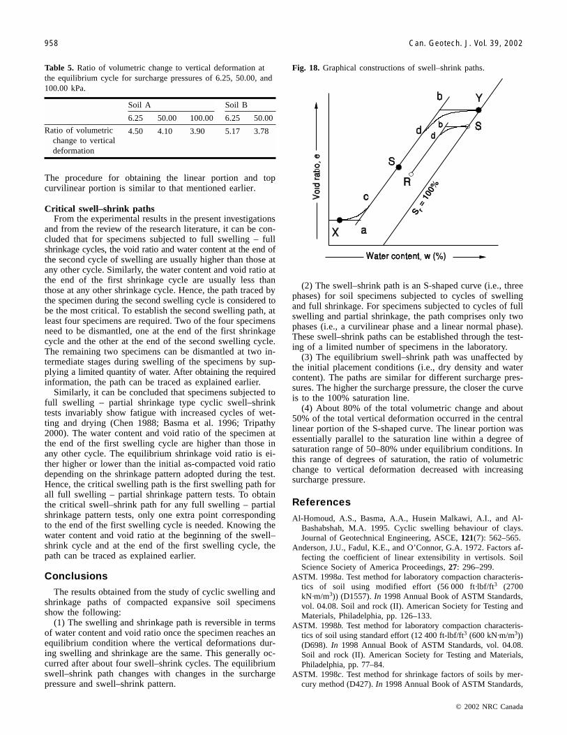
The procedure for obtaining the linear portion and topcurvilinear portion is similar to that mentioned earlier.

Critical swell–shrink pathsFrom the experimental results in the present investigations

and from the review of the research literature, it can be con-cluded that for specimens subjected to full swelling – fullshrinkage cycles, the void ratio and water content at the end ofthe second cycle of swelling are usually higher than those atany other cycle. Similarly, the water content and void ratio atthe end of the first shrinkage cycle are usually less thanthose at any other shrinkage cycle. Hence, the path traced bythe specimen during the second swelling cycle is considered tobe the most critical. To establish the second swelling path, atleast four specimens are required. Two of the four specimensneed to be dismantled, one at the end of the first shrinkagecycle and the other at the end of the second swelling cycle.The remaining two specimens can be dismantled at two in-termediate stages during swelling of the specimens by sup-plying a limited quantity of water. After obtaining the requiredinformation, the path can be traced as explained earlier.

Similarly, it can be concluded that specimens subjected tofull swelling – partial shrinkage type cyclic swell–shrinktests invariably show fatigue with increased cycles of wet-ting and drying (Chen 1988; Basma et al. 1996; Tripathy2000). The water content and void ratio of the specimen atthe end of the first swelling cycle are higher than those inany other cycle. The equilibrium shrinkage void ratio is ei-ther higher or lower than the initial as-compacted void ratiodepending on the shrinkage pattern adopted during the test.Hence, the critical swelling path is the first swelling path forall full swelling – partial shrinkage pattern tests. To obtainthe critical swell–shrink path for any full swelling – partialshrinkage pattern tests, only one extra point correspondingto the end of the first swelling cycle is needed. Knowing thewater content and void ratio at the beginning of the swell–shrink cycle and at the end of the first swelling cycle, thepath can be traced as explained earlier.

Conclusions

The results obtained from the study of cyclic swelling andshrinkage paths of compacted expansive soil specimensshow the following:

(1) The swelling and shrinkage path is reversible in termsof water content and void ratio once the specimen reaches anequilibrium condition where the vertical deformations dur-ing swelling and shrinkage are the same. This generally oc-curred after about four swell–shrink cycles. The equilibriumswell–shrink path changes with changes in the surchargepressure and swell–shrink pattern.

(2) The swell–shrink path is an S-shaped curve (i.e., threephases) for soil specimens subjected to cycles of swellingand full shrinkage. For specimens subjected to cycles of fullswelling and partial shrinkage, the path comprises only twophases (i.e., a curvilinear phase and a linear normal phase).These swell–shrink paths can be established through the test-ing of a limited number of specimens in the laboratory.

(3) The equilibrium swell–shrink path was unaffected bythe initial placement conditions (i.e., dry density and watercontent). The paths are similar for different surcharge pres-sures. The higher the surcharge pressure, the closer the curveis to the 100% saturation line.

(4) About 80% of the total volumetric change and about50% of the total vertical deformation occurred in the centrallinear portion of the S-shaped curve. The linear portion wasessentially parallel to the saturation line within a degree ofsaturation range of 50–80% under equilibrium conditions. Inthis range of degrees of saturation, the ratio of volumetricchange to vertical deformation decreased with increasingsurcharge pressure.

References

Al-Homoud, A.S., Basma, A.A., Husein Malkawi, A.I., and Al-Bashabshah, M.A. 1995. Cyclic swelling behaviour of clays.Journal of Geotechnical Engineering, ASCE, 121(7): 562–565.

Anderson, J.U., Fadul, K.E., and O’Connor, G.A. 1972. Factors af-fecting the coefficient of linear extensibility in vertisols. SoilScience Society of America Proceedings, 27: 296–299.

ASTM. 1998a. Test method for laboratory compaction characteris-tics of soil using modified effort (56 000 ft·lbf/ft3 (2700kN·m/m3)) (D1557). In 1998 Annual Book of ASTM Standards,vol. 04.08. Soil and rock (II). American Society for Testing andMaterials, Philadelphia, pp. 126–133.

ASTM. 1998b. Test method for laboratory compaction characteris-tics of soil using standard effort (12 400 ft-lbf/ft3 (600 kN·m/m3))(D698). In 1998 Annual Book of ASTM Standards, vol. 04.08.Soil and rock (II). American Society for Testing and Materials,Philadelphia, pp. 77–84.

ASTM. 1998c. Test method for shrinkage factors of soils by mer-cury method (D427). In 1998 Annual Book of ASTM Standards,

© 2002 NRC Canada


Fig. 18. Graphical constructions of swell–shrink paths.

Soil A Soil B

6.25 50.00 100.00 6.25 50.00

Ratio of volumetricchange to verticaldeformation

4.50 4.10 3.90 5.17 3.78

Table 5. Ratio of volumetric change to vertical deformation atthe equilibrium cycle for surcharge pressures of 6.25, 50.00, and100.00 kPa.



vol. 04.08. Soil and rock (II). American Society for Testing andMaterials, Philadelphia, pp. 157–162.

Basma, A.A., Al-Homoud, A.S., Malkavi, A.I.H., and Al-Bashabshah, M.A. 1996. Swelling–shrinkage behaviour of natu-ral expansive clays. Applied Clay Science, 11: 211–227.

Brasher, B.R., Franzmier, D.P., Valassis, V., and Davidson, S.E.1966. Use of Saran resin to coat natural soil clods for bulk-density and water-retention measurements. Soil Science, 101(2):108.

Bureau of Indian Standards. 1970. Classification and identificationof soils for general engineering purposes (IS 1498). Bureau ofIndian Standards Institute, New Delhi.

Chen, F.H. 1988. Foundations on expansive soils. 2nd ed. ElsevierScience Publishing Co., Inc., New York.

Crescimanno, G., and Provenazano, G. 1999. Soil shrinkage char-acteristic curve in clay soils: measurement and prediction. SoilScience Society of America Journal, 63: 25–32.

Crilly, M.S., Driscoll, R.M., and Chandler, R.J. 1992. Seasonalground water movement observation in an expansive clay site inthe U.K. In Proceedings of the 7th International Conference onExpansive Soils, Dallas, Tex., pp. 313–318.

Croney, D., and Coleman, J.D. 1954. Soil structure in relation tosoil suction (pF). Journal of Soil Science, 5(1): 75–84.

Dasog, G.S., Acton, D.F., Mermuth, A.R., and De Jong, E. 1988.Shrink–swell potential and cracking in clay soils of Saskatche-wan. Canadian Journal of Soil Science, 68: 251–260.

Day, R.W. 1994. Swell–shrink behaviour of expansive compactedclay. Journal of Geotechnical Engineering, ASCE, 120(3): 618–623.

Day, R.W. 1999. Geotechnical and foundation engineering designand construction. McGraw-Hill Co., New York.

Dif, A.F., and Blumel, W.F. 1991. Expansive soils with cyclic dry-ing and wetting. ASTM Geotechnical Testing Journal, 14(1):96–102.

Erol, A.O. 1992. Insitu and laboratory measured suction parame-ters for prediction of swell. In Proceedings of the 7th Interna-tional Conference on Expansive Soils, Dallas, Tex., pp. 30–32.

Fleureau, J.-M., Kheirbek-Saoud, S., Soemitro, R., and Taibi, S.1993. Behavior of clayey soils on drying–wetting paths. Cana-dian Geotechnical Journal, 30: 287–296.

Fredlund, D.G., and Rahardjo, H. 1993. Soil mechanics for unsatu-rated soils. John Wiley & Sons, Inc., New York.

Gromko, G.J. 1974. Review of expansive soils. Journal of theGeotechnical Engineering Division, ASCE, 100(6): 667–687.

Haines, W.B. 1923. The volume changes associated with variationsof water content in soil. Journal of Agricultural Science, 13:296–310.

Hanafy, E.A.D.E. 1991. Swelling/shrinkage characteristic curve ofdesiccated expansive clays. ASTM Geotechnical Testing Jour-nal, 14(2): 206–211.

Ho, D.Y.F., Fredlund, D.G., and Rahardjo, H. 1992. Volumechange indices during loading and unloading of an unsaturatedsoil. Canadian Geotechnical Journal, 29: 195–207.

Holtz, W.G., and Gibbs, G.J. 1956. Engineering properties of ex-pansive clays. Transactions of the American Society of Civil En-gineers, 121: 641–677.

Jennings, J.E.B., and Kerrich, J.E. 1962. The heaving of buildingsand the associated economic consequences with particular refer-ence to the Orange Free State goldfields. Civil Engineer inSouth Africa, Transactions of the South African Institute ofCivil Engineering, 4(11): 221–248.

Kezdi, A. 1980. Hand book of soil mechanics. Vol. 2. Soil testing.Elsevier Scientific Publishing Co., Amsterdam.

Marinho, F.A.M., and Stuermer, M. 1999. The influence of thecompaction energy on the SWCC of a residual soil. In Advancesin unsaturated geotechnics. Geotechnical Special Publication,ASCE, pp. 125–141.

McIntyre, D.S., and Loveday, J. 1968. Problems of determinationof soil density and moisture properties from natural clods. SoilScience, 105(4): 232–236.

McKeen, R.G., and Hamberg, D.J. 1981. Characterization of ex-pansive soils. Transportation Research Record 790, pp. 73–78.

Mitchell, J.K. 1976. Fundamentals of soil behaviour. John Wiley &Sons, Inc., New York.

Mitchell, A.R., and van Genuchten, M.Th. 1992. Shrinkage of bareand cultivated soil. Soil Science Society of America Journal, 56:1036–1042.

Nelson, J.D., and Miller, D.J. 1992. Expansive soils problems andpractice in foundation and pavement engineering. John Wiley &Sons, Inc., New York.

Padmanabha, J.R. 1988. Some studies on engineering behaviour ofblack cotton soils as affected by climatic conditions. Ph.D. the-sis, Indian Institute of Science, Bangalore, India.

Parcher, J.V., and Liu, P.D. 1965. Some swelling characteristics ofcompacted clays. Journal of the Soil Mechanics and Founda-tions Division, ASCE, 91(SM3): 1–17.

Popescu, M. 1980. Behaviour of expansive soils with crumb struc-tures. In Proceedings of the 4th International Conference on Ex-pansive Soils, Denver, Colo., Vol. 1, pp. 158–171.

Ring, W.E. 1966. Shrink–swell potentials of soils. Highway Re-search Record 119, National Academy of Sciences – NationalResearch Council Publication 1360, pp. 17–21.

Sitharam, T.G., Sivapulliah, P.V., and Subba Rao, K.S. 1995.Shrinkage behaviour of compacted unsaturated soils. In Pro-ceedings of the 1st International Conference on UnsaturatedSoils, Paris, pp. 195–200.

Songyu, L., Heyuan, L., Peng, J., and Yanjun, D. 1998. Approachto cyclic swelling behaviour of compacted clays. In Proceedingsof the 2nd International Conference on Unsaturated Soils,Beijing, China, Vol. 2, pp. 219–225.

Stirk, G.B. 1954. Some aspects of soil shrinkage and the effect ofcracking upon water entry into the soil. Australian Journal ofAgricultural Research, 5: 279–291.

Subba Rao, K.S. 2000. Swell–shrink behaviour of expansive soils —geotechnical challenges. Indian Geotechnical Journal, 30(1): 1–68.

Subba Rao, K.S., and Satyadas, G.C. 1985. Measurement of volu-metric and linear shrinkage of black cotton soil. ASTMGeotechnical Testing Journal, 8(2): 66–70.

Subba Rao, K.S., and Satyadas, G.C. 1987. Swelling potentialswith cycles of swelling and partial shrinkage. In Proceedings ofthe 6th International Conference on Expansive Soils, New Delhi,India, Vol. 1, pp. 137–147.

Subba Rao, K.S., Rao, S.M., and Gangadhara, S. 2000. Swellingbehaviour of desiccated clay. ASTM Geotechnical Testing Jour-nal, 23(2): 193–198.

Tripathy, S. 2000. Cyclic swell–shrink behaviour of compacted ex-pansive soils. Ph.D. thesis, Indian Institute of Science,Bangalore, India.

Tunny, J. 1970. The influence of Saran resin coatings on swellingof natural soil clods. Soil Science, 109(4): 254–256.

Warkentin, B.P., and Bozozuk, M. 1961. Shrinkage and swellingproperties of two Canadian clays. In Proceedings of the 5th In-ternational Conference on Soil Mechanics and Foundation Engi-neering. Dunod, Paris, pp. 851–855.

Yong, R.W., and Warkentin, B.P. 1975. Soil properties and behav-iour. Elsevier Scientific, New York.

© 2002 NRC Canada

Tripathy et al. 959



Documents

Water content – void ratio swell–shrink paths of compacted ...soilvision.com/subdomains/unsaturatedsoil.com/Docs... · The swelling potential of an expansive soil is commonly