WASHINGTON UNIVERSITY - cse.wustl.edulegrand/dissertation.pdf · Robert Hampton LeGrand III May 2008 Washington University St. Louis, Missouri Professor Ron K. Cytron, Chairperson

WASHINGTON UNIVERSITY

Sever InstituteSchool of Engineering and Applied Science

Department of Computer Science and Engineering

Dissertation Examination Committee:Ron K. Cytron, Chair

Steven BramsJeremy BuhlerRobert PlessItai Sened

Aaron Stump

COMPUTATIONAL ASPECTS OF APPROVAL VOTING

AND DECLARED-STRATEGY VOTING

by

Robert Hampton LeGrand III, B.S., M.C.S.

A dissertation presented to the

Graduate School of Arts and Sciences

of Washington University in partial fulfillment

of the requirements for the degree of

Doctor of Philosophy

May 2008

St. Louis, Missouri

Acknowledgements

I will always be grateful to my research advisor, Ron K. Cytron, for his guidance, perspective,

encouragement and patience. He has been a pleasure to work with and a great help in exploring

and evaluating research ideas and directions. I am passionate about this research and feel very

lucky to have had the opportunity to work with him on it.

I also appreciate Steven J. Brams of NYU for his groundbreaking ideas that inspired much of this

work. He has been extraordinarily encouraging and generous with his time, and it was a great

honor to have him serve on my dissertation examination committee.

I would also like to thank the rest of my committee, Jeremy Buhler, Robert Pless, Itai Sened and

Aaron Stump, for their time and valuable comments, and the DOC Group, especially James

Brodman, Delvin Defoe, Morgan Deters, Scott Friedman, Richard Hough, Tobias Mann and Justin

Thiel, who made it such a fun lab to work in.

Finally, for their love, support and pride, I owe my parents, Robert H. LeGrand Jr. and Marsha

LeGrand, the most thanks of all.

Robert Hampton LeGrand III

Washington University, St. Louis

May 2008

i

Contents

Acknowledgements . . . . . . . . . . . . . . . . . . . . . . . . . . . . . . . . . . . . . . . . i

List of Tables . . . . . . . . . . . . . . . . . . . . . . . . . . . . . . . . . . . . . . . . . . . . v

List of Figures . . . . . . . . . . . . . . . . . . . . . . . . . . . . . . . . . . . . . . . . . . . vi

Preface . . . . . . . . . . . . . . . . . . . . . . . . . . . . . . . . . . . . . . . . . . . . . . . . ix

1 Introduction and Background . . . . . . . . . . . . . . . . . . . . . . . . . . . . . . . 1

1.1 Declared-Strategy Voting . . . . . . . . . . . . . . . . . . . . . . . . . . . . . . . . . 1

1.2 Approval voting . . . . . . . . . . . . . . . . . . . . . . . . . . . . . . . . . . . . . . . 4

1.3 Notions of sincerity . . . . . . . . . . . . . . . . . . . . . . . . . . . . . . . . . . . . . 5

1.4 Existing strategic approaches . . . . . . . . . . . . . . . . . . . . . . . . . . . . . . . 7

1.5 Computationally simple approval strategies . . . . . . . . . . . . . . . . . . . . . . . 9

2 Manipulation (or, What You Will) . . . . . . . . . . . . . . . . . . . . . . . . . . . . 13

2.1 Notions of manipulation . . . . . . . . . . . . . . . . . . . . . . . . . . . . . . . . . . 14

2.1.1 Election specification . . . . . . . . . . . . . . . . . . . . . . . . . . . . . . . . 15

2.1.2 Ballot choice of voters . . . . . . . . . . . . . . . . . . . . . . . . . . . . . . . 15

2.2 Manipulation decision problems . . . . . . . . . . . . . . . . . . . . . . . . . . . . . . 16

2.3 Strategic insincerity and DSV . . . . . . . . . . . . . . . . . . . . . . . . . . . . . . . 19

2.3.1 An NP-hard result . . . . . . . . . . . . . . . . . . . . . . . . . . . . . . . . . 19

ii

2.4 Generalizing hardness results to approval voting . . . . . . . . . . . . . . . . . . . . 21

2.5 Summary of contributions . . . . . . . . . . . . . . . . . . . . . . . . . . . . . . . . . 22

3 DSV and Approval-Rating Polls . . . . . . . . . . . . . . . . . . . . . . . . . . . . . . 23

3.1 Approval ratings and their aggregation . . . . . . . . . . . . . . . . . . . . . . . . . . 24

3.1.1 Examples of approval rating polls . . . . . . . . . . . . . . . . . . . . . . . . . 24

3.1.2 Formulation . . . . . . . . . . . . . . . . . . . . . . . . . . . . . . . . . . . . . 25

3.1.3 Aggregating approval ratings . . . . . . . . . . . . . . . . . . . . . . . . . . . 27

3.2 Rationally optimal strategy for Average aggregation . . . . . . . . . . . . . . . . . . 31

3.2.1 Strategy for a final, omnisicent voter . . . . . . . . . . . . . . . . . . . . . . . 31

3.2.2 Equilibrium for n strategic voters . . . . . . . . . . . . . . . . . . . . . . . . . 33

3.3 Multiple equilibria can exist . . . . . . . . . . . . . . . . . . . . . . . . . . . . . . . . 36

3.4 At most one equilibrium average rating can exist . . . . . . . . . . . . . . . . . . . . 37

3.5 At least one equilibrium always exists . . . . . . . . . . . . . . . . . . . . . . . . . . 39

3.6 Average-Approval-Rating DSV . . . . . . . . . . . . . . . . . . . . . . . . . . . . . . 47

3.6.1 A new class of rating systems . . . . . . . . . . . . . . . . . . . . . . . . . . . 49

3.6.2 Monotonicity of AAR DSV . . . . . . . . . . . . . . . . . . . . . . . . . . . . 51

3.6.3 AAR DSV is immune to Average-style strategy . . . . . . . . . . . . . . . . . 52

3.6.4 AAR DSV never rewards insincerity . . . . . . . . . . . . . . . . . . . . . . . 55

3.7 A simpler AAR DSV algorithm . . . . . . . . . . . . . . . . . . . . . . . . . . . . . . 58

3.8 Parameterizing AAR DSV . . . . . . . . . . . . . . . . . . . . . . . . . . . . . . . . . 62

3.9 Evaluation of AAR DSV systems . . . . . . . . . . . . . . . . . . . . . . . . . . . . . 64

3.10 Generalizations to more dimensions . . . . . . . . . . . . . . . . . . . . . . . . . . . . 67


4 Comparing Approval Strategies for DSV . . . . . . . . . . . . . . . . . . . . . . . . 71

4.1 The space of approval ballots . . . . . . . . . . . . . . . . . . . . . . . . . . . . . . . 73

4.2 A new declared strategy for approval voting . . . . . . . . . . . . . . . . . . . . . . . 73

iii

4.3 Evaluating approval strategies . . . . . . . . . . . . . . . . . . . . . . . . . . . . . . . 74

4.3.1 Evaluating election states directly . . . . . . . . . . . . . . . . . . . . . . . . 74

4.3.2 Evaluating election states by looking ahead . . . . . . . . . . . . . . . . . . . 77

4.4 General results using the Merrill election-state metric . . . . . . . . . . . . . . . . . 81

4.4.1 Comparing strategies A and T in the three-alternative case . . . . . . . . . . 81

4.4.2 Comparing strategies A and J in the three-alternative case . . . . . . . . . . 84

4.4.3 Comparing strategies T and J in the three-alternative case . . . . . . . . . . 86

4.4.4 Comparing strategies A and Z in the three-alternative case . . . . . . . . . . 89

4.4.5 Comparing strategies A and T in the four-alternative case . . . . . . . . . . . 92

4.4.6 A general result for strategy A using the Merrill metric . . . . . . . . . . . . 99

4.5 General results using the branching-probabilities election-state metric . . . . . . . . 100

4.5.1 A general result for strategy A using the branching-probabilities metric . . . 102


5 Fixed-size Minimax . . . . . . . . . . . . . . . . . . . . . . . . . . . . . . . . . . . . . . 106

5.1 Introduction . . . . . . . . . . . . . . . . . . . . . . . . . . . . . . . . . . . . . . . . . 106

5.1.1 Related work . . . . . . . . . . . . . . . . . . . . . . . . . . . . . . . . . . . . 108

5.2 Definitions and notation . . . . . . . . . . . . . . . . . . . . . . . . . . . . . . . . . . 109

5.3 NP-hardness and approximation algorithms . . . . . . . . . . . . . . . . . . . . . . . 110

5.4 Local search heuristics for fixed-size minimax . . . . . . . . . . . . . . . . . . . . . . 112

5.4.1 A framework for FSM heuristics . . . . . . . . . . . . . . . . . . . . . . . . . 112

5.4.2 Evaluating the heuristics . . . . . . . . . . . . . . . . . . . . . . . . . . . . . 114

5.5 Manipulation . . . . . . . . . . . . . . . . . . . . . . . . . . . . . . . . . . . . . . . . 116

5.6 Future work . . . . . . . . . . . . . . . . . . . . . . . . . . . . . . . . . . . . . . . . . 119

5.7 Acknowledgements . . . . . . . . . . . . . . . . . . . . . . . . . . . . . . . . . . . . . 120


References . . . . . . . . . . . . . . . . . . . . . . . . . . . . . . . . . . . . . . . . . . . . . . 121

iv

Vita . . . . . . . . . . . . . . . . . . . . . . . . . . . . . . . . . . . . . . . . . . . . . . . . . . 125

v

List of Tables

5.1 Largest approximation ratios found for local search heuristics . . . . . . . . . . . . . 115

5.2 Average approximation ratios found for local search heuristics . . . . . . . . . . . . . 116

5.3 Average scaled performance of local search heuristics . . . . . . . . . . . . . . . . . . 117

vi

List of Figures

1.1 Outline of DSV operation . . . . . . . . . . . . . . . . . . . . . . . . . . . . . . . . . 2

1.2 Approval strategy Z . . . . . . . . . . . . . . . . . . . . . . . . . . . . . . . . . . . . 10

1.3 Approval strategy T . . . . . . . . . . . . . . . . . . . . . . . . . . . . . . . . . . . . 11

1.4 Approval strategy B . . . . . . . . . . . . . . . . . . . . . . . . . . . . . . . . . . . . 11

1.5 Approval strategy J . . . . . . . . . . . . . . . . . . . . . . . . . . . . . . . . . . . . 12

3.1 RMSE, varying a and fixing b = 0.5000 . . . . . . . . . . . . . . . . . . . . . . . . . . 65

3.2 RMSE, varying a and fixing b = 0.4820 . . . . . . . . . . . . . . . . . . . . . . . . . . 66

3.3 RMSE, fixing a = 0.3647 and varying b . . . . . . . . . . . . . . . . . . . . . . . . . . 67

3.4 Φ0.3647,0.4820(~v) vs. v scatterplot . . . . . . . . . . . . . . . . . . . . . . . . . . . . . 68

4.1 Approval strategy A . . . . . . . . . . . . . . . . . . . . . . . . . . . . . . . . . . . . 74

vii

ABSTRACT OF THE DISSERTATION

Computational Aspects of Approval Voting

and Declared-Strategy Voting

by


May 2008

Washington University

St. Louis, Missouri

Professor Ron K. Cytron, Chairperson

Computational social choice is a relatively new discipline that explores issues at the intersection of

social choice theory and computer science. Designing a protocol for collective decision-making is

made difficult by the possibility of manipulation through insincere voting. In approval voting

systems, voters decide whether to approve or disapprove available alternatives; however, the specific

nature of rational approval strategies has not been adequately studied. This research explores

aspects of strategy under three different approval systems, from chiefly a computational viewpoint.

While traditional voting systems elicit only the outcome of a voter’s strategic thinking, a

Declared-Strategy Voting (DSV) system accepts such strategies directly and applies them

according to the voter’s preferences over the available alternatives. Ideally, when rational strategies

are employed on behalf of the voters, voters are discouraged from expressing insincere preferences.

Approval voting is a natural fit for use with DSV, but, unlike for the common plurality voting

system, there is no extant theory regarding the most effective approval strategies in a DSV

context. We propose such a theory.

Approval-rating polls already serve an important role in assaying the views of an electorate on

some subject of interest. Sites such as Rotten Tomatoes and Metacritic.com collect and display the

results of approval-rating polls for movies and games. Moreover, sites such as Amazon and eBay

collect approval ratings to estimate the worthiness of their buyers and sellers. In these polls, a

rational voter’s approval or disapproval will sometimes be insincere so as to move the result in a

desired direction. A nonmanipulable protocol would allow indication of a voter’s ideal outcome

and would never reward an insincere such indication. We present and analyze a large new class of

such nonmanipulable protocols motivated by the DSV concept.

The minimax procedure is a multiwinner form of approval voting that aims to maximize the

satisfaction with the outcome of the least satisfied voter. Unfortunately, computing the minimax

winner set is computationally hard. We propose an approximation algorithm for this problem, a

framework for polynomial-time heuristics that perform very well in practice, and a preliminary

analysis of strategic voting under minimax.

Preface

Computer technology has been made to serve mankind in many ways. Today computers make

simple many tasks that were previously more difficult or even impossible. Many public elections

remained largely mechanical with little help from computers well into the information age, but

computerized voting systems have received rapidly increasing attention since 2000 [40, 31]. Much

has been written [3, 41] about real and theoretical computerized systems that verify voters, collect

ballots and count votes, but there has been relatively little exploration of the possibility of

computers assisting voters with making strategic voting decisions.

When voting in elections, voters often find that a sincere ballot is unlikely to be the most effective

one. For example, imagine an election for a single winner with three alternatives in which each

voter is allowed to give a vote to one alternative. If a specific voter prefers A to B and B to C, but

estimates that A is likely to finish a distant third, that voter may decide that choosing B is more

likely to have a positive effect on the outcome. The outcome of an election can depend greatly on

the extent and quality of this kind of strategically insincere voting in the electorate.

But choosing the most effective ballot is not always straightforward for a human voter, especially

when the voter has little information on the alternatives’ relative strengths. Even when rich

information regarding the current vote totals and other voters’ preferences is available, the most

effective ballot—that is, the one that is likeliest to lead to the optimal reachable outcome—may

not be obvious to a human voter. What is needed, then, is a system that will carry out the

calculations required to find an optimally effective ballot for the voter. Such a system would make

both naıvely sincere and sophisticated voters equally effective.

x

1

Chapter 1

Introduction and Background

In this chapter we will introduce important concepts and review previous work relevant to our

research directions.

1.1 Declared-Strategy Voting

In 1996, Lorrie Cranor and Ron K. Cytron [23] described a hypothetical voting system they called

Declared-Strategy Voting (DSV). DSV arose from the desire to elicit richer, more sincere1

preferences from voters by using that information to find a winning alternative in such a way that

voters would be unlikely to gain a superior result by submitting insincere preferences.

DSV can be seen as a meta-voting system, in that it uses voters’ expressed preferences among

alternatives to vote rationally in their stead in repeated simulated elections. The repeated

simulated elections are run according to the rules of some underlying voting protocol, which can be

any protocol that accepts any kind of ballots and uses them to elect one winner. Cranor [22]

explored using DSV with plurality, but DSV, as a meta-voting system, could conceivably work

with any voting protocol.

1Unfortunately, the terms “sincerity” and “manipulation” are used with little consistency in the social-choiceliterature. We will review the various uses of these terms and define the senses in which we use them, “sincerity” inthis chapter and “manipulation” in the next.

2

ballotvector

.

..

.

.

.

stateelectionvisible

ballot

current

ballotprocessorexecutor

statecalculator

program

program

program

generators

("voters")program

winner(s)

program

judge

selector

Figure 1.1: Outline of DSV operation

As depicted in Figure 1.1, a DSV system maintains a ballot vector and an election state through a

series of rounds. The ballot vector is empty at the beginning of the election and is updated after

each voter’s program executes to hold all of the current ballots. The election state consists of a

vector of rational numbers, one for each alternative in the election, that correspond to the current

vote totals. It is updated using the ballot vector; the DSV mode (described below) of the election

determines when and how that update takes place.

In a DSV election, a voter submits not a ballot but a DSV program. A program is essentially a

function that takes some set of updated information about an election in progress as input and

uses it to decide on a ballot to vote in the voter’s stead. In the most general case, the program

itself can be any algorithm taking in all input related to the election in progress, such as all ballots

previously voted, the contents of all other submitted programs and the number of ballots processed

so far. But few real-world voters are sophisticated enough to provide such a program directly.

In this research, a program is assumed to consist of a set of a voter’s cardinal preferences (or

utility ratings) over the alternatives and a rule, known as a declared strategy, that generates an

appropriate ballot at that point in the election. The cardinal preferences (ratings) are constrained

to rational numbers between 0 and 1 inclusively; a rating measures the utility of an alternative to a

voter—the degree to which that alternative’s victory is desirable. For example, if alternatives are

candidates for public office, a rating can be interpreted as an estimate of the proportion of issues

on which the voter and candidate agree, weighted by importance to the voter and likelihood of

3

relevance during the period of representation. Ratings are assumed to scale linearly and otherwise

behave as von Neumann–Morgenstern utilities [57].

The declared strategy is a precisely defined algorithm that takes as input only the current election

state, the voter’s cardinal preferences and the voter’s previously voted ballot; notably, the declared

strategy has no knowledge of when it will next be executed or which voters’ programs have already

executed. The declared strategy is expressed by submitting a well defined algorithm or choosing

one from a predetermined list. The aim of the declared strategy is to maximize the result of the

election according to the voter’s submitted cardinal preferences.

Once all programs are submitted, a selector selects a program to be executed. The selector

effectively determines the order in which the programs are executed. The ith round consists of the

ith execution of each program and the processing of the resulting ballots. Each program must be

selected i times before any program may be selected in round (i + 1), but apart from that

restriction the selection is random and impartial.

An executor interprets the selected program and runs it with the current election state as input to

produce a ballot as output. Only a finite number of computational steps is allowed to the program;

if the program has not finished execution in the allotted number of steps, it is halted and an empty

ballot results. This number can be made large enough for any reasonable program to complete

comfortably but must be finite to guarantee progress and eventual completion of the election. The

declared strategies considered in this research will be polynomial-time algorithms and will be

assumed to finish in the allotted number of steps.

The ballot that is generated is then passed on to the ballot processor, which checks whether the

ballot is well formed according to the underlying voting protocol. For example, if plurality were

being used as the underlying voting protocol, the ballot [1, 1, 0] would be rejected since plurality

only allows one vote for at most one alternative. If the ballot is accepted as valid, the ballot

processor then integrates it into the current ballot vector; the election’s mode determines how that

integration occurs.

The two modes described by Cranor [22] are ballot-by-ballot mode and batch mode. In this

research, a mode can further be non-cumulative (like Cranor’s modes) or cumulative, giving four

4

possible DSV modes: ballot-by-ballot, batch, cumulative ballot-by-ballot and cumulative batch. If

an election is run in one of the cumulative modes, the ballot processor adds a newly voted ballot to

the ballot vector; if a non-cumulative mode is used, the ballot processor uses a newly voted ballot

to replace that voter’s previously voted ballot, so that each voter has at most one ballot in the

ballot vector at any time.

The state calculator uses the current ballot vector to update the election state; the election’s mode

also determines how this update occurs. If the system is in a ballot-by-ballot mode, whether

cumulative or not, the ballots in the ballot vector are summed and the summed vector replaces the

previous election state after each ballot is processed. In a batch mode, the summed vector replaces

the previous election state only after the last ballot of each round, that is, when each program has

been executed the same number of times.

The underlying voting protocol (e.g., plurality), the mode (e.g., non-cumulative batch mode) and

the number of rounds (e.g., 30) are the only settings needed to specify a DSV voting system fully.

1.2 Approval voting

Approval voting is a simple single-winner voting protocol. It was used in the Republic of Venice

and to elect the pope in the thirteenth through seventeenth centuries [47], and it was rediscovered

independently in the 1970s by several authors, including Guy Ottewell [44], Robert Weber [59] and

Steven Brams and Peter Fishburn [13]. Under approval voting each voter may approve any subset

of the available alternatives, effectively recording a yes or no vote for each alternative. In this

version of approval voting that elects exactly one of a finite number of discrete alternatives, the

one alternative that receives the most approval votes is chosen as the winner.

We propose that approval voting is a good candidate for use with DSV. DSV with plurality has

been previously explored [22]; a plurality vote that can be expected to maximize a voter’s utility of

the eventual outcome often deserts a favorite alternative to vote for another. More generally, it is

sometimes rational to vote for A (and not B) even though B is preferred to A. Under approval

voting a voter could vote fully for the same compromise alternative while also supporting fully his

5

or her favorite. Assuming the favorite has a nonzero chance of winning, doing so will further

increase expected utility of the outcome, so perhaps approval voting induces less insincere voting

by some measure. For example, unlike under plurality, it may never be rational under approval

voting to vote for A and not B when B is preferred to A.

1.3 Notions of sincerity

Under most voting systems, insincere voters can gain an advantageous outcome. Specifically, for

most systems it sometimes happens that the most effective ballot contradicts a voter’s true

preferences. For example, if a voter’s true preferences are for A over B and B over C and the other

votes total 40 for A, 50 for B and 50 for C, the single most effective plurality ballot is one for B. It

is reasonable to consider such a ballot insincere because it expresses a pairwise preference for B

over A, contradicting the voter’s sincere preferences.

Standard since Arrow’s seminal impossibility result [4] in the realm of voting theory is to assume

ordinal preferences and ordinal ballots. In such a world, a sincere ordinal ballot is simply one that

exactly reflects the voter’s ordinal preferences. (Of course, if voters may have tied preferences, then

they must be allowed to vote tied rankings to maintain the possibility of sincerity.)

This notion of sincerity can be generalized to cardinal preferences and ballots in different ways, but

we focus on two in this work.2 First, If voters are assumed to have Von Neumann–Morgenstern [57]

(cardinal and linearly scalable) utilities over the available alternatives, where p(i) is a voter’s

cardinal preference (utility) for alternative i, and any particular allowed ballot is interpreted to

assign a rating v(i) to each alternative, then at least two notions of sincerity can be easily defined:

strong sincerity A ballot is strongly sincere if and only if, for all alternatives i and j,

v(i) > v(j)←→ p(i) > p(j).

2We assume that any voting protocol accepts ballots that can be interpreted to assign some rating to each al-ternative. For example, plurality only allows assigning the rating 1 to one alternative and 0 to the rest; approvalvoting allows assigning either 0 or 1 to each alternative; ranked-ballot voting systems allow any assignment of rationalnumbers to the alternatives, where alternatives given higher ratings are taken to be ranked ahead of those given lowerratings. So cardinal-ratings ballots nicely generalize a large class of ballots without loss of information, though eachvoting protocol has its own set of allowed ballots.

6

weak sincerity A ballot is weakly sincere if and only if, for all alternatives i and j,

v(i) > v(j) −→ p(i) > p(j). (This definition is equivalent to the definition of sincerity given

by Brams and Fishburn [14, p. 29].)

So, for example, a voter with sincere utilities over three alternatives [1, 0.8, 0] might vote the

approval ballot [1, 1, 0]; such a ballot is weakly but not strongly sincere. (Note that no strongly

sincere approval ballot exists for a voter with tri- or multichotomous [14, p. 17] preferences such as

these.)

Merrill [38, p. 80] outlines different notions of sincerity specifically for approval voting. He

describes an approval ballot that is not even weakly sincere as a skipping ballot, as such a ballot’s

approvals “skip” down the voter’s preference ordering. For example, a voter who prefers A to B to

C to D but approves only A and C is voting a skipping ballot. By this definition, an approval

ballot is weakly sincere if and only if it is not skipping.

Notice that, if a voter knows exactly how every other voter will vote, a skipping ballot cannot be

uniquely best. In other words, for any skipping ballot, there is some weakly sincere approval ballot

that obtains an outcome which is no worse. For example, if C and D are tied for the win, then, for

the voter mentioned above, approving B as well as A and C can only help; if A and B are tied for

the win, then approving C as well as A can only hurt.

Also specifically for approval voting, Merrill defines “pure” sincerity:

pure sincerity An approval ballot is purely sincere if and only if, for all k alternatives i,

p(i) >�

j p(j)

k −→ v(i) = 1 and p(i) ≤�

j p(j)

k −→ v(i) = 0.

Note that, according to this definition, if a voter assigns equal utilities to all alternatives, a purely

sincere ballot would disapprove all alternatives.

Gibbard [30] and Satterthwaite [53] independently showed that, for any voting protocol that treats

ballots and alternatives symmetrically, the most effective ballot is not always strongly sincere when

there are at least three alternatives.3 The two protocols most often given as examples to which the

3The Gibbard–Satterthwaite theorem considers protocols with fully ranked input, so every weakly sincere ballot isalso strongly sincere. The theorem also effectively applies to protocols that accept ballots with tied ranks, but saysonly that strong (and not weak) sincerity must sometimes be violated by a rationally strategic voter.

7

Gibbard–Satterthwaite theorem does not apply are random ballot (a ballot is selected randomly;

the highest rated alternative on it wins) and random runoff (two alternatives are randomly chosen;

the one preferred to the other on more ballots wins). Neither treats ballots and alternatives

symmetrically and thus are not generally considered appropriate for real-world elections.

So, every reasonable voting protocol sometimes rewards departing from strong sincerity, but, as we

will further see below in section 1.4, approval voting can be said never to reward departing from

weak sincerity. Other well-known protocols such as plurality, Hare (STV) [8] and Borda [51]

cannot make the same claim.

1.4 Existing strategic approaches

While a DSV program can in general be any piece of code that a voter submits, rational

program-writers will be attempting to generate a ballot that takes their cardinal preferences into

account. Accordingly, we have assumed that a program consists of (1) cardinal preferences over the

alternatives and (2) a declared strategy, which uses the election state and the cardinal preferences

to find a ballot that is deemed likeliest to maximize the election result according to the preferences.

Several authors have investigated concepts very similar to what we call declared strategies. Brams

and Fishburn [14, ch. 7] explore a concept they call the “poll assumption”, which models changes

in voters’ strategy given the election state (the “poll”) under both plurality and approval voting.

One variation, which they call the “Poll Assumption (Approval)”, is defined on page 115 (they use

the term “strategy” to mean what we call “ballot”):

After the poll, voters will adjust their voting strategies [ballots] to distinguish between

the top two candidates, as indicated by the poll [election state], if they prefer one of

these candidates to the other and their sincere, pre-poll strategies did not involve

voting for exactly one of these choices. Given that they are not indifferent between the

top two candidates in the poll, they will vote after the poll for their preferred candidate

and all candidates preferred to him (if any). [14]

8

Below (Figure 1.4) we will call this poll assumption “strategy B” and define it more precisely.

Brams and Fishburn give examples that show alternatives being hurt and helped when voters

strategically respond to poll information using this poll assumption; we will see that there exist

other reasonable ways to respond to polls that may result in different equilibria when all voters use

them.

Chapter 5 of Merrill [38] constructs a general theory of strategy under uncertainty (where nothing

is known about the alternatives’ relative chances of winning) and risk (where each alternative’s

probability of winning is assumed to be known or estimated). His approach to strategy under risk

assumes knowledge of pivot probabilities tij , where tij is the probability that, given that the

election results in a tie between two alternatives, alternatives i and j are the participants in the

tie. He uses these pivot probabilities to calculate a strategic value for each alternative: the

expected benefit according to the voter’s cardinal preferences of adding one vote for that

alternative. He then finds, of all valid ballots, the one that maximizes the total strategic value.

Cranor [22] offers a theory of rational declared strategies and applies it especially to plurality DSV

elections. She outlines several approaches to transforming an election state into pivot probabilities,

the most prominent of which essentially treats each alternative’s proportion of the votes in the

current election state as the mean of a Gaussian distribution of that alternative’s eventual

proportion of the votes, assumes some particular variance for the distribution (S2, which could be

seen as a measure of uncertainty in the current vote totals), and then calculates the probability

that each pair of alternatives will eventually tie for the win. When voters are randomly sampled to

obtain the distribution, the variance can be modeled according to the Gaussian error of estimate

based on the fraction of the electorate sampled so far. The resulting pivot probabilities are then

used as by Merrill to find an optimal plurality ballot.

Cranor’s approach attempts to define rational strategy directly by making certain reasonable

assumptions but does not atttempt to show that, in practice, the strategies found lead to better

results for voters that use them than any other strategy approaches.

9

1.5 Computationally simple approval strategies

Several existing styles of designing effective declared strategies were described in section 1.4. Some,

such as the strategies of Brams and Fishburn, were intended to model approximately how typical

real-world voters might vote when they have poll information. Such strategies are desirable for

DSV for three reasons: they are based on results that have already appeared in the literature, they

can be described simply enough for a human voter to understand easily and they can be executed

quickly by a computer regardless of the numbers of voters and alternatives. Several such strategies

are defined below; they all are computationally simple and can be found in extant literature. All of

them always result in a weakly sincere approval ballot, essentially setting some cardinal cutoff over

which alternatives are approved and under which they are disapproved, so skipping ballots never

result.

To simplify the description of approval strategies, we will assume that DSV is run in

non-cumulative batch mode, which means that the election state visible to a voter in round r + 1

depends only on the ballots submitted in round r.

Notation varies widely in the literature, but we will describe election situations using the following.

Any election has k alternatives numbered from 1 to k and n voters numbered from 1 to n. For

notational convenience, � n is defined as the set {z ∈ � : 1 ≤ z ≤ n} (the integers between 1 and n)

and � m...n is defined as the set {q ∈ � : m ≤ q ≤ n} (the rational numbers between m and n).

The voters’ sincere cardinal preferences are represented as the function p : � n× � k→ � , where

p(i, j) = voter i’s cardinal preference for alternative j. The ballots submitted throughout the DSV

rounds are represented as the function b : � n× � k× � → � 0...1, where b(i, j, r) = voter i’s vote for

alternative j in round r; b(i, j, 0) = 0 for all i and j.4 The election states are represented as the

function s : � k× � → � 0...n, where s(j, r) =∑n

i=1 b(i, j, r), alternative j’s vote total at the end of

round r.

The approval strategies defined below calculate the ballot for voter v at round r + 1; that is, given

v and r, they calculate b(v, i, r + 1) (= 1 for approval and 0 for disapproval) for each alternative i.

4Here � denotes the set of nonnegative integers: � = {n ∈ � : n ≥ 0}.

10

It will be useful to define two more functions. Topy(r) is the set of the y leading alternatives

according to round r’s election state:

Topy(r) = {i : |{j : s(i, r) < s(j, r)}| < y}

PSumy(v, r) is the sum of voter v’s cardinal preferences of the alternatives in Topy(r):

PSumy(v, r) =∑

j∈Topy(r)

p(v, j)

Also, we define the set C(r) of “contending” alternatives at round r to be {i : s(i, r) ≥ x} where x

is as large as possible with the constraint that |C(r)| ≥ 2 for all r.

One of the simplest strategies effectively ignores the election state and assumes that each

alternative has an equal probability of winning the election, approving each alternative the voter

rates higher than his average rating over all alternatives. We call this approach strategy Z and

define it precisely in Figure 1.2. Note that the definition uses Top and PSum to make clear its

similarities with those of the other strategies we will consider, but as only Topk and PSumk are

used the effect is to compare each alternative’s utility to the average utility over all the

alternatives, so the election state is effectively ignored.

Figure 1.2: Approval strategy Z

For voter v voting in round r + 1,

• for each alternative i:

– approve alternative i if and only if p(v, i) · |Topk(r)| > PSumk(v, r)

Strategy Z is always purely sincere according to Merrill’s definition above. It is also equivalent to

the optimal approval strategy according to the Laplace method for making decisions under

uncertainty Merrill [38] gives in chapter 5.

Another strategy based only on a voter’s preferences and the alternatives’ current vote totals is

often given by advocates of approval voting as a good rule of thumb for real-world approval

elections [47, p. 196]. Mike Ossipoff [43] wrote, “In Plurality, if you’re sure that Smith & Jones will

be the top 2 votegetters, then obviously you should vote for whichever of those 2 you prefer to the

11

other. In Approval, vote for him and for everyone whom you like better.” Equivalently, an

approval cutoff is placed just below the preferred of the top two alternatives. We call this approach

strategy T and define it more precisely in Figure 1.3.

Figure 1.3: Approval strategy T



– find smallest y such that p(v, i) · |Topy(r)| 6= PSumy(v, r) (y = k if none)

– if y ≤ 2:

∗ approve alternative i if and only if p(v, i) · |Top1(r)| > PSum1(v, r)and p(v, i) · (|Top2(r)| − |Top1(r)|) > PSum2(v, r)− PSum1(v, r)

– else:

∗ approve alternative i if and only if p(v, i) · |Topy(r)| > PSumy(v, r)

The first of the two strategies Brams and Fishburn [14] describe we will call strategy B; the second

we will call strategy J. Strategy B takes as input not only a voter’s preferences and the

alternatives’ current vote totals but also the voter’s previous ballot. We use the description of the

Poll Assumption (Approval) and the ensuing examples to inspire the precise definition of Strategy

B in Figure 1.4. Strategy B will change a voter’s ballot only when necessary to differentiate among

the contending alternatives.

Figure 1.4: Approval strategy B


• if r > 0:

– b−1 = voter v’s ballot cast in round r

• else:

– b−1 = ballot found by applying strategy Z

• if b−1 includes all alternatives in C(r) or none of them:

– apply strategy T

• else:

– use voter v’s previously cast ballot

12

Brams and Fishburn describe a variation on their Poll Assumption (Approval) on page 120, which

can be generalized to what we call strategy J and define precisely in Figure 1.5. Strategy J will vote

a purely sincere ballot whenever doing so would differentiate among the contending alternatives.

Figure 1.5: Approval strategy J


• if the ballot found by using strategy Z includes all alternatives in C(r) ornone of them:

– apply strategy T

• else:

– apply strategy Z

It is worth pointing out that the approval strategies presented above (plus strategy A, defined in

Figure 4.1) effectively use only the ordinal preferences of a voter. In other words, any cardinal

preferences that impose the same preference order over the alternatives will result in identical

ballots if any of these strategies is used. Therefore they can be used equally effectively whether

preference input consists of cardinal utilities or a (perhaps partial) ordering of the alternatives.

In chapter 4 we will compare the effectiveness of these approval strategies according to different

evaluation metrics.

13

Chapter 2

Manipulation (or, What You Will)

The developers [23] of Declared-Strategy Voting (DSV) elections posited that their election

protocol would force rational voters to specify cardinal preferences sincerely, while still acting in

the best interest of each voter at the moment that voter must pick an alternative. In this way they

were attempting to avoid the possibility of manipulation, which is an unfortunately grossly

overloaded term in voting literature. In section 2.1, we examine the nature of manipulation in

voting systems, settling on a definition that suits our goals in this chapter.

The act of voting requires brain activity, and the Church–Turing hypothesis [18, 55, 33] says that

activity can be captured by a program. That program P takes in basically three things: the

election protocol, the voter’s feelings about the alternatives and the voter’s expectations

concerning how everybody else will vote.

The protocol specifies the manner in which the election will be conducted: it is a mathematical

function from a list of ballots to one or more winners. We assume that voters cannot (will not) act

until the protocol has been set. With the protocol established, a voter will act based upon the

other two factors: that voter’s feelings about the alternatives, and that voter’s expectation

concerning how everybody else will vote.

If we examine only those two factors, then literature can be summarized as follows.

14

sincerity If P is based only on the voter’s feelings, ignoring how others might vote, then P is

acting sincerely. However, it is well known [30, 53] that acting so directly on the voter’s

feelings may result in a provably worse outcome for the voter in terms of who wins the

election. In that sense, P is generally irrational and a better outcome is obtainable through

strategic behavior.

irrationality If P is based only on how others vote, ignoring how the voter feels about the

alternatives, then P is by definition irrational. Examples include bandwagon and underdog

voting [22].

strategy If P takes into account both how the voter feels and how others might vote, then P is

acting strategically (even though P may happen to output a ballot that is sincere in some

sense). If P can be shown, by some objective measure perhaps similar to those explored in

chapter 4, to obtain outcomes influenced favorably by the voter’s preferences, then P can be

said to be acting rationally.

In summary of DSV, most voting protcols compel voters to act strategically to be rational. DSV

elections hope to cause voters to act sincerely to be rational—by moving the voter’s insincere

program into the DSV system itself.

2.1 Notions of manipulation

One of a democracy’s goals is to conduct elections that are fair, in the sense that no individual has

an undue influence on an election’s outcome. Such influence is loosely called manipulation, and we

next examine various mechanisms by which an individual (or group of collaborating individuals)

can influence an election’s outcome. Of course, every voter has the potential to influence an

election’s outcome; otherwise, voting would be a futile activity. In discussions of manipulation, it is

therefore important to discern the nature of influence and to establish the conditions under which

an individual’s influence is unfair.

15

2.1.1 Election specification

Those who specify an election and its protocol have the ability to manipulate an election. For

example, election officials could overtly exclude an alternative, either so that alternative cannot win

or because, if included, that alternative would prevent the election of a more desirable alternative

due to a vote-splitting effect [42]. They could also affect the outcome by determining the set of

allowed voters [9], perhaps allowing only those who support the favored outcome or excluding

those who support strong rival outcomes. More subtly, if the election officials have the chance to

choose an election protocol, then one can be chosen so as to obtain (probabilistically or for certain)

a given outcome [52], or at least one that is less likely to give a particular undesirable outcome.

2.1.2 Ballot choice of voters

More common in the literature is to identify the manipulation opportunities of voters themselves.

Intuitively speaking, manipulation by a voter occurs when he or she changes a ballot in the

expectation of effecting a superior outcome; in this research, we will use only this notion of

manipulation. But when, more precisely, can manipulation be said to have occurred? We will

consider two possibilities:

1. A voter or group of voters, using all available information, decides whether a specific

alternative can be made to win with at least a given probability and, if so, votes in such a

way to elect that alternative. (Such voters are acting strategically in the sense defined above.)

2. A voter submits an insincere ballot that results in an election outcome better for that voter

than the one that would have resulted if he or she had voted sincerely. (Insincerity can be

reckoned by weak sincerity or strong sincerity as defined in chapter 1.)

These two notions of manipulation address strategy and insincerity, respectively.

The first is useful to consider when a voter is deciding how to vote; if a corresponding decision

problem is shown to be computationally hard, it may be reasonable to expect voters to default to

voting sincerely. Decision problems of this sort will be investigated in the next section.

16

The second identifies when a voter has “gamed the system”; it is what many social-choice authors

mean when they describe a voting system as manipulable. (By this definition, a voting system is

nonmanipulable when any rationally strategic ballot is sincere.) One design motivation for DSV

was to encourage the submission of sincere preferences. In particular, it was hoped that

ballot-by-ballot mode, by randomizing voter order, would deter the submission of insincere

preferences; if a voter determines that insincere preferences will gain a superior outcome given one

voter order, the same preferences may be unlikely to gain the same outcome given another voter

order.

2.2 Manipulation decision problems

There have already been attempts to characterize the difficulty of manipulating voting systems.

The following decision problem is a generalization of several in the literature.

Existence of Probably Winning Coalition Ballots (EPWCB)

INSTANCE: Set of alternatives A and a distinguished member a of A; set of weighted

cardinal-ratings ballots BV ; the weights of a set of ballots BU which have not been

cast; probability 0 < π ≤ 1

QUESTION: Does there exist a way to cast the ballots BU so that a has at least

probability π of winning the election with the ballots BV ∪ BU?

EPWCB is perhaps best explained by presenting its interesting subproblems.

Existence of a Winning Ballot (EWB)

INSTANCE: Set of alternatives A and a distinguished member a of A; set of

cardinal-ratings ballots B

QUESTION: Does there exist a way to cast a ballot b0 so that a wins the election with

the ballots B ∪ {b0} outright?

EWB is identical to the decision problem Existence of a Winning Preference (EWP)

presented and analyzed by Bartholdi, Tovey and Trick [7], except that EWP uses ordinal ballots,

17

standard for the literature in this area. EWB essentially looks at a manipulation opportunity from

the point of view of a DSV voter coming last in the voter order: All other ballots are considered to

be cast, fixed and known, and the question is whether there is a ballot that the ultimate voter can

cast to cause the election of a certain alternative. The assumed situation is very much like that of

a DSV program computing the final ballot of a round on behalf of its voter. Bartholdi et al.’s

reasoning for using EWP is that it assumes all relevant information is available—if one can show

that, for a given voting system, EWP is computationally hard, then manipulating that voting

system must be hard when less information is available.

Bartholdi, Tovey and Trick are able to show that a polynomial-time algorithm exists for solving

EWP in general for a large class of voting protocols, which includes plurality and approval voting.

However, they present a protocol they call Second-Order Copeland for which solving EWP is

NP-hard, and in a later paper Bartholdi and Orlin [8] show that EWP is also NP-hard for the

single transferable vote (STV) in its single-winner version—also known as Hare, Instant Runoff

Voting (IRV) or the alternative vote. But when the number of alternatives is held constant, a

polynomial-time algorithm solving EWP exists even for these protocols, so EWP’s NP-hardness

depends on a large slate of alternatives.

Existence of Winning Coalition Ballots (EWCB)

INSTANCE: Set of alternatives A and a distinguished member a of A; set of weighted

cardinal-ratings ballots BV ; the weights of a set of ballots BU which have not been cast

QUESTION: Does there exist a way to cast the ballots BU so that a wins the election

outright?

EWCB is Constructive Coalitional Weighted Manipulation (CCWM), introduced by

Conitzer and Sandholm [20], with cardinal instead of ordinal ballots as input. EWCB is a

generalization of EWB that, surprisingly, is NP-hard for many protocols even given a constant

number of alternatives.

Note that EWB and EWCB ask whether a specific alternative can be made to win. The more

general and perhaps more intuitively useful problem of finding a voter’s most-liked alternative that

can be made to win is not significantly harder: one would simply test each alternative in decending

18

order of cardinal preference; when alternative a can be made to win, alternatives not preferred to a

need not be considered.

Conitzer and Sandholm [21] described three “tweaks” that, when added to a voting protocol, such

as plurality or the Borda count [51], make that protocol computationally hard to manipulate. All

three use a “preround” to determine a set of alternatives to be eliminated before the voting

protocol is executed. The simplest, called a deterministic preround, publishes a pairing of the

alternatives before the ballots are collected; for each pair, the loser of the pairwise comparison

between them according to the ballots is eliminated—if the number of alternatives is odd, one

alternative survives without a comparison—and the original protocol, such as plurality or Borda, is

executed on the ballots over the remaining alternatives. Adding this deterministic preround to a

large class of protocols, including plurality and Borda, renders them NP-hard to manipulate in the

sense of EWP.

The second preround tweak pairs the alternatives randomly after the ballots have been collected; it

makes a protocol #P-hard to manipulate, but in a special sense: Instead of asking whether a

specific alternative a can be made to win, as in EWP, it asks whether a can be made to win with

some given probability 0 < π ≤ 1.

Existence of a Probably Winning Ballot (EPWB)

INSTANCE: Set of alternatives A and a distinguished member a of A; set of

cardinal-ratings ballots B; probability 0 < π ≤ 1

QUESTION: Does there exist a way to cast a ballot b0 so that a has at least

probability π of winning the election with the ballots B ∪ {b0}?

Perhaps the nondeterminism of DSV’s ballot-by-ballot mode has a similar effect on manipulation,

either making it computationally difficult in this probabilistic sense or making it so that any

manipulation that would work given one voter order would backfire for some other voter order.

Recall from section 1.3 that the Gibbard–Satterthwaite theorem proves that any voting protocol,

including a meta-voting system like DSV, that treats ballots and alternatives symmetrically is

manipulable by strategic voters, and, further, that the two protocols (random ballot and random

19

runoff) most often given as examples to which the Gibbard–Satterthwaite theorem does not apply

have a large nondeterministic component. Could it be that there is generally a tradeoff between

manipulability and determinism?

2.3 Strategic insincerity and DSV

One motivation for the design of DSV was to elicit the submission of sincere preferences by having

the system strategize for the voter. The hope is that the voter’s declared strategy will cast ballots

in such a way that the eventual outcome of the election is optimized from the voter’s point of view,

giving the voter no reason to try to gain a better outcome by submitting insincere preferences. In

other words, one hopes that the declared strategy will do everything in its power to make the

winner of the election as good as possible so that submitting false preferences can only backfire.

Unfortunately, the Gibbard–Satterthwaite theorem dashes hope that any reasonable voting system

will be found that is immune to strategic insincerity in all voting situations with at least three

alternatives. So even DSV, assuming no bias towards some voters or some alternatives is built in,

will have cases with opportunities for manipulation by submitting insincere cardinal preferences.

Different DSV systems—those with different underlying voting protocols and in different

modes—may in practice present manipulation opportunities to voters more or less often. For

example, it may be much easier to find an election example where plurality DSV rewards the

submission of insincere cardinal preferences than for approval DSV. But even if DSV is sometimes

manipulable, one might expect it to be generally difficult to find the preferences that would

manipulate successfully.

2.3.1 An NP-hard result

As it turns out, DSV can be shown to be computationally hard to manipulate in a certain sense.

EWB, the version of Bartholdi’s and Orlin’s [8] EWP with cardinal-preference ballots, captures the

relevant notion of manipulability. They showed that EWP is NP-hard for Hare, the single-winner

form of STV.

20

Hare takes ordinal ballots as input. The ballots are counted in a series of elimination rounds. In

the first round, only the top-rank votes are counted. The alternative with the smallest top-rank

total is eliminated from the ballots, possibly adding to other alternatives’ top-rank totals. This

step is repeated until exactly one winner is left.

If a specific choice of declared strategy is forcibly made for all voters, DSV in batch mode with

plurality as the underlying voting protocol can be made to simulate Hare. If the imposed declared

strategy is carefully chosen, DSV can be made to select the winner that Hare would given the

ranked ballots corresponding to the voters’ expressed cardinal preferences. So if voters are not free

to choose their own declared strategies, DSV can be made NP-hard to manipulate.

Theorem 2.3.1. If a declared strategy can be imposed on the voters, so that they submit only their

cardinal preferences over the alternatives, DSV can be made to be NP-hard to manipulate in the

EWB sense.

Proof. We will always elect the Hare winner according to the ordinal ballots implied by the voters’

cardinal preferences if we use DSV in batch mode with one-vote plurality as the underlying

protocol and the following strategy for all voters:

vote for alternative i such that pi = max(pj : sj ≥ t)

where

t =

min(U \ {min(U)}) if |U | > 1

min(U) if |U | = 1

0 if |U | = 0

and

U = {sj : sj > 0}

In the first round of the batch DSV election, when (∀i) si = 0, the imposed strategy will vote for

each voter’s favorite alternative, just as in the first round of counting a Hare election. In

subsequent DSV rounds, as long as |U | > 1 (there remain more than one uneliminated alternative),

all voters vote for their most preferred alternative with a vote total at least t, a threshold set at

the second-smallest vote total, effectively eliminating the alternative(s) with the lowest vote totals

21

among the uneliminated alternatives. When |U | = 1 (only one alternative has a nonzero vote

total), every voter votes for that alternative. The resulting election state does not change

afterward, and that alternative, which is the Hare winner, thus wins the DSV election.

Bartholdi and Orlin [8] proved that Hare (the single-winner version of STV) is NP-hard to

manipulate in the Existence of a Winning Preference (EWP) sense. EWP is a subproblem

of Existence of a Winning Ballot (EWB), so Hare is NP-hard to manipulate in the EWB

sense as well. Since batch DSV with the above imposed strategy is equivalent to Hare, DSV can be

made NP-hard to manipulate in the EWB sense.

So DSV is NP-hard to manipulate in the general case. But what does this mean? It means only

that there is no algorithm that runs in time polynomial in the number of alternatives and the

number of voters that is guaranteed to find a set of preferences that guarantees a given outcome.

It does not mean that DSV is necessarily hard to manipulate in every case. There may be a simple

heuristic that often (if not always) finds preferences that will manipulate successfully, or one that

tends to lead to a better outcome than blind sincerity. It also does not imply that manipulating

DSV is necessarily easy or hard when declared strategies can be freely chosen.

2.4 Generalizing hardness results to approval voting

Conitzer and Sandholm [19] showed that CCWM is in P for plurality for any constant number of

alternatives but NP-hard for Borda and veto voting with three or more alternatives. (For every

voting system under consideration, CCWM is in P when the number of alternatives is limited to

two.) CCWM takes ranked ballots as input, so approval voting cannot be applied to CCWM. But

EWCB works with approval voting; it is simply CCWM with cardinal-preference input. EWCB

can be seen to be in P for approval voting by using the same manipulation algorithm that works

for plurality: Approve on all ballots only a, the distinguished alternative that is to be made to win.

There is a way to make a win if and only if this strategy makes a win.

22

2.5 Summary of contributions

In this research, we have accomplished the following.

1. Proved that manipulating DSV in general is NP-hard by describing a plurality DSV system

that imposes a specified declared strategy on all voters in such a way that the Hare winner is

elected.

2. Provided a polynomial-time algorithm for solving EWCB for approval voting.

23

Chapter 3

DSV and Approval-Rating Polls

We see DSV as a way to reduce or eliminate manipulation by voters’ insincerity by embracing

manipulation itself. By strategizing for the voter, a “perfect” DSV system would encourage sincere

indication of preferences. In the next chapter we will investigate questions regarding the

manipulability of DSV in the general case, where it is used to elect one of a static set of

alternatives over which voters may hold any preferences. But the DSV framework can be used in

other contexts. In particular, if certain assumptions are made about the available alternatives and

the voters’ preferences among them, stronger results regarding DSV are possible.

In this chapter we will investigate applying DSV to the problem of selecting a number from a

specified range of numbers. We will show that this new application of DSV achieves the original

goal of DSV: It eliminates the possibility of manipulation by making insincere voting no more

effective than sincere voting. Intuitively, this is possible because we assume that voters can only

have certain kinds of preferences over the possible outcomes, effectively reducing the space of

possible elections. For example, if the alternatives consist of the rational numbers between 0 and 1,

we can justifiably assume each voter’s preferences over the considered range to be single-peaked. In

other words, we can assume that no voter will prefer a over b and c over b if a < b < c.

24

This application of DSV may have fewer uses in real-world elections than a more general DSV

system that allows arbitrary voter preferences over alternatives, but it can be seen as an

illustration of the power of DSV in principle and an etude for the further study of DSV.

3.1 Approval ratings and their aggregation

Approval ratings are one mechanism that communities can use to offer incentive and reward for

good behavior or service. The prospect of feedback following a given interaction presumably

increases the accountability of that interaction for all parties involved. Publication of approval

ratings then enables appropriate consequences to follow from positive or negative experiences.

It is interesting, however, to consider the form in which approval ratings can and should be

published. While the greatest detail is afforded by publication of each participant’s response to an

approval rating poll, the resulting volume is typically unacceptable for the purposes of

summarizing an electorate’s experience. Thus, some form of aggregation is typically performed on

approval ratings, and the result of that aggregation is then announced as the result of the poll.

In this chapter we consider several forms of aggregation and we show that some methods can

reward insincerity while others cannot. We next provide several examples of approval rating

systems and formulate a general form of an approval rating poll.

3.1.1 Examples of approval rating polls

Subscribers and observers of media frequently learn of the results of approval rating polls that

attempt to discern how strongly a participating electorate endorses a person or a position of

interest. For example, approval ratings concerning the performance of the United States President

are published throughout a presidency; following events or policy decisions that affect an

electorate, such polls are often conducted as a means of evaluating the electorate’s support for the

President’s actions.

25

As another example, several web sites post varous forms of approval ratings for movies and games.

Specifically, Rotten Tomatoes [2] posts the results of two polls for each movie:

• Each review from a set of accredited critics is turned into approval (fresh rating) or

disapproval (rotten rating) of the reviewed material, in terms of whether the material merits

viewing. The percentage of fresh reviews is reported as the movie’s Tomatometer. In effect,

each review is turned into a 0 or 1 value, and the Tomatometer is the average of those values

expressed as a percentage. Putative viewers might consult a movie’s Tomatometer value to

determine whether they should see that movie.

• Each critic can also rate a movie’s overall quality on a 1–10 scale. Rotten Tomatoes then

publishes the average of all such ratings. Similarly, Metacritic [1] computes a weighted

average of its accredited reviewers’ approval ratings for a given movie, supplied on a 0–100

scale.

Finally, consider the electronic marketplace, in which participants are asked to rate the honesty

and effectiveness of merchants and customers. Sites such as eBay poll their participants concerning

how strongly they approve of the behavior of the marketplace members they encounter in

transactions. Upon completion of a transaction, the involved parties are asked to rate each other.

An aggregation of an indvidual’s approval ratings is posted for public view, so that members can

consider such information before engaging that individual in a transaction.

Based on the above, some approval ratings are formulated more incrementally than others. For

example, the ratings published by Rotten Tomatoes and Metacritic are collected and then analyzed

en masse, while the approval rating of an eBay participant (merchant or customer) can be updated

after every interaction involving that participant. As we show below, knowledge concerning how

others approve of a given issue can influence a particpant’s expressed approval rating.

3.1.2 Formulation

We next define a general instance of an approval rating poll to facilitate presentation of our results.

26

• An electorate of n participants is polled. Based on the participants’ response and the

aggregation protocol at hand, the result of the poll will be published as a rational number in

the interval [0, 1].

• Each participant i has in mind a sincere preference rating ri, 0 ≤ ri ≤ 1 that can be

construed as that participant’s dictatorial preference. The tuple of all participants’ sincere

ratings is denoted by the vector ~r.

We further make the reasonable assumption that voter i’s preferences are single-peaked and

non-plateauing: a voter’s utilities for the outcomes are monotonically decreasing when

moving away from ri in either direction. It follows, for example, that any voter that prefers

0.2 to 0.5 must also prefer 0.5 to 0.8. More formally:

– If a < b ≤ ri, then voter i must prefer b to a;

– If ri ≤ c < d, then voter i must prefer c to d.

Based on the above, ri sufficiently characterizes a voter’s outcome utilities for our purposes.

• Each participant i has also in mind a probability density function pi that models the

probabilistic outcome of the poll, excluding i’s rating. For the purposes of this chapter, the

outcome from i’s point of view is simply an expected value oi. While a more general

treatment could be the subject of future work, we therefore assume pi is the Dirac δ function:

pi = δ(t− oi) =

∞ if t = oi

0 if t 6= oi

with the area under pi summing by definition to unity.

– In situations where preference data accrues incrementally and the poll’s results are

updated continually, oi is readily available before the ith participant expresses approval.

Such is the case in eBay when a buyer provides an approval rating for a merchant.

– In other cases, preliminary polls or other information sources may provide sufficient

information to provide a likely value for oi.

While estimations of oi could be inaccurate, faulty or based on purposefully falsified

information, the presence of such information can affect an electorate as discussed below.

27

• Finally, voter i participates in the poll by expressing a rating preference of vi, which may or

may not be the same as ri. In fact, we are particularly interested in situations where vi 6= ri

due to pi. For example, the expression of an individual’s approval rating could well be

affected by knowledge (perceptions, estimations, or actualities) of how others approve of the

issue at hand. For example, consider an eBay customer who undertakes a transaction with a

highly approved merchant. If the customer becomes disgruntled with the merchant, then the

customer’s resulting rating of the merchant might be overly negative, precisely because of the

merchant’s otherwise high rating.

The tuple of all expressed approval ratings is denoted by the vector ~v.

This chapter considers an approach that can account for, mitigate, or prevent the use of insincerity

to increase a participant’s effectiveness in an approval rating poll.

3.1.3 Aggregating approval ratings

The results of an approval rating poll are typically reported by an aggregation procedure that is

disclosed a priori. In this section, we consider two popular aggregation schemes: average and

median.

Average aggregation Here, the result of the approval rating poll is computed as the average of

the participants’ expressed approval ratings:

v =

∑nj=1 vj

n

While the Average aggregation function is sensitive to each voter’s input, it has an important

disadvantage: Voters can often gain by voting insincerely. For example, the 1983 film Videodrome

has five critics’ ratings on Metacritic. If we assume that these critics rated the film sincerely (that

each would prefer that the average rating of the film be his or her rating), we have

~r = [0.4, 0.7, 0.8, 0.8, 0.88]

28

If these preferences are actually expressed sincerely in an Average aggregation context, then we

have

~v = [0.4, 0.7, 0.8, 0.8, 0.88]

and the Average aggregation yields 0.716.

Consider voter 5, whose ideal outcome is r5 = 0.88. That voter could achive a better outcome by

not expressing the sincere preference v5 = 0.88 and instead voting v5 = 1. The resulting Average

aggregation yields the outcome 0.74, which, being closer to 0.88, is preferred by voter 5 to 0.716.

Median aggregation (n odd) Another possible aggregation function computes a median of ~v:

v is a value that satisfies

|{i : v < vi}| ≤n

2and |{i : v > vi}| ≤

n

2

or, equivalently,

|{i : v < vi}| ≤n

2≤ |{i : v ≤ vi}|

The above definition does not necessarily prescribe a unique aggregation when n is even; we

address this issue below.

According to the median voter theorem [10, 24], when n is odd, Median aggregation becomes the

unique, Condorcet-compliant [38] rating system, yielding a result that is preferred by some

majority of voters to every other outcome.

Unfortunately, Median aggregation can effectively ignore almost half of the voters. In other words,

majority rule can mean majority tyranny. Given the following tuple of votes

~v = [0, 0, 0, 1, 1]

the 1-voters are effectively ignored when the median, 0, is chosen as the outcome. Majority

tyranny could be quite undesirable for polls of this type, especially when the goal of aggregating

ratings is to represent a satisfactory consensus for all voters. The Average outcome of the above

tuple, 0.4, arguably provides such a much better consensus.

29

In contrast with Average aggregation, Median aggregation is nonmanipulable by insincere

voters—at least when n is odd: a voter i can never improve the outcome from his or her point of

view by voting vi 6= ri.

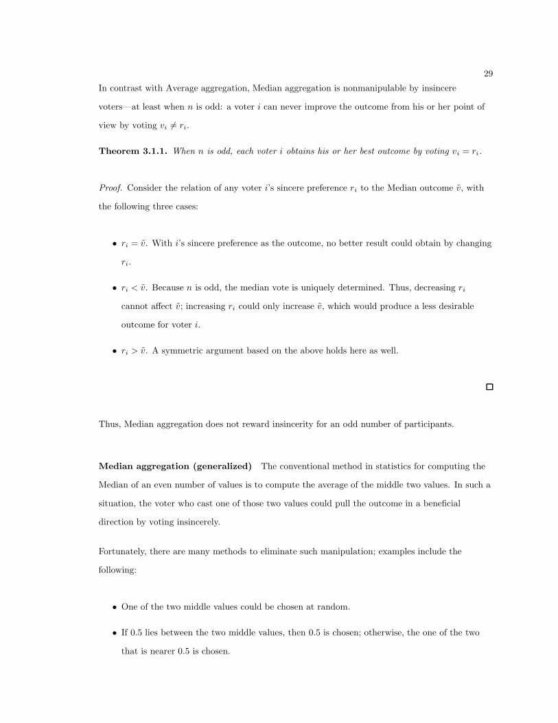
Theorem 3.1.1. When n is odd, each voter i obtains his or her best outcome by voting vi = ri.

Proof. Consider the relation of any voter i’s sincere preference ri to the Median outcome v, with

the following three cases:

• ri = v. With i’s sincere preference as the outcome, no better result could obtain by changing

ri.

• ri < v. Because n is odd, the median vote is uniquely determined. Thus, decreasing ri

cannot affect v; increasing ri could only increase v, which would produce a less desirable

outcome for voter i.

• ri > v. A symmetric argument based on the above holds here as well.

Thus, Median aggregation does not reward insincerity for an odd number of participants.

Median aggregation (generalized) The conventional method in statistics for computing the

Median of an even number of values is to compute the average of the middle two values. In such a

situation, the voter who cast one of those two values could pull the outcome in a beneficial

direction by voting insincerely.

Fortunately, there are many methods to eliminate such manipulation; examples include the

following:

• One of the two middle values could be chosen at random.

• If 0.5 lies between the two middle values, then 0.5 is chosen; otherwise, the one of the two

that is nearer 0.5 is chosen.

30

Note that the outcome v given by any of these median functions minimizes∑

i|vi − v|, in contrast

to the average function, v, which minimizes∑

i(vi − v)2.

Without losing nonmanipulability, the Median function can be generalized to give the outcome

bv where |{i : bv < vi}| ≤ bn ≤ |{i : bv ≤ vi}|

for any 0 ≤ b ≤ 1. (In this notation, the b is intended as a parameter modifying the tilde.) If bn is

an integer, there may be more than one 0 ≤ φ ≤ 1] that satisfies

|{i : φ < vi}| ≤ bn ≤ |{i : φ ≤ vi}|

In that case, define Φ as the set of all such φ. Then

bv ≡

min(Φ) if b < min(Φ)

b if min(Φ) ≤ b ≤ max(Φ)

max(Φ) if max(Φ) b

b if b ∈ Φ

max(Φ) if (∀φ ∈ Φ) φ < b

This order-statistic outcome equals max(~v) when b = 0, the third quartile when b = 14 , the Median

outcome when b = 12 , the first quartile when b = 3

4 and min(~v) when b = 1.

Summary For an approval-rating poll, the choice of aggregation mechanism affects the nature of

the outcome and the reward for voter insincerity. The Average aggregation outcome can reward

insincerity, but the outcome provides a reasonable consensus of the electorate. On the other hand,

Median aggregation does not reward insincerity, but it allows for tyranny by a majority.

31

3.2 Rationally optimal strategy for Average aggregation

As shown in section 3.1, Average aggregation can reward insincerity. In this section, we develop a

rationally optimal strategy: a computation by which a voter can achieve a result as close as

possible to that voter’s prefered outcome. As before, we assume an eletorate in which n voters will

express preferences. We begin by considering a rationally optimal strategy from the perspective of

a final, omniscient voter. We then consider the behavior of a system in which all voters use a

rationally optimal strategy.

To facilitate exposition and analysis of our results, we begin by generalizing the scale on which

preferences are expressed as follows. In an [m, M ]-Average poll, voters are allowed to express

preference ratings in the interval [m, M ], m ≤ 0, 1 ≤M . We continue to assume that sincere

preference ratings are in the interval [0, 1]; the expanded range is therefore intended to allow voters

more room to manipulate the outcome. We also assume that preferences are aggregated by

computing the Average of the voters’ expressed preferences.

3.2.1 Strategy for a final, omnisicent voter

Consider a (−∞, +∞)-Average poll in which voter vn is the last voter to express an approval

rating, and in which all other voters vote their sincere preference ratings: (∀i 6= n) vi = ri. If voter

n can see the expressed approval ratings of all voters, then the ideal outcome for voter n (v = rn)

can be realized by voting

vn = rnn−∑

j 6=n

rj

More generally, in an [m, M ]-Average poll, voter n should express vn to move the outcome as close

to rn as possible:

vn = min

max

rnn−∑

j 6=n

rj , m

, M

(3.1)

The above is the rationally optimal strategy for voter n in an [m, M ]-Average approval rating poll.

32

As an example, consider the [0, 1]-Average system with sincere preferences from the Videodrome

example above:

~r = [0.4, 0.7, 0.8, 0.8, 0.88]

After all other voters express their sincere preferences, v5’s rationally optimal preference rating is

given by

v5 = min

max

r5n−∑

j 6=5

rj , 0

, 1

= min (max (0.88 · 5− (0.4 + 0.7 + 0.8 + 0.8), 0) , 1)

= 1 (3.2)

achieving an outcome v of 0.74. No other choice for v5 would achieve an outcome v closer to

r5 = 0.88.

After voter n has voted using Equation 3.1, exactly one of the following is true.

1. v < rn and vn = M

2. v = rn

3. v > rn and vn = m

In each case, either voter n’s ideal outcome rn has been realized, or voter n has moved the

outcome as close to rn as is immediately possible. Based on the three cases above, no other choice

for rn has that property.

Moreover, in each of the above three cases, v ∈ [0, 1] even though vn ∈ [m, M ]. Recall that each

sincere preference, including rn, is in the interval [0, 1]. In case (1), we have v < rn ≤ 1. Thus we

need only show 0 ≤ v: Since v is computed as the average of n− 1 numbers in the interval [0, 1]

and one number (vn = M) ≥ 1, we obtain 0 ≤ v. A symmetric argument holds for case (3). Case

(2) follows directly since v = rn.

33

3.2.2 Equilibrium for n strategic voters

We have thus far allowed only voter n to use a rationally optimal strategy, requiring all other

voters to express their sincere approval ratings. We now consider the properties of the more

practical [m, M ]-Average system in which each voter i uses a rationally optimal strategy to

compute an expressed approval rating, based on i’s sincere approval rating ri and on the expressed

votes of all other voters. When each voter i establishes vi, other voters may wish to update their

expressed approval ratings.

Returning to the Videodrome example, in which minimum vote m = 0 and maximum vote M = 1,

we again have sincere preferences

~r = [0.4, 0.7, 0.8, 0.8, 0.88]

Hypothetically, let us say initial votes are assumed to be sincere:

~v = [0.4, 0.7, 0.8, 0.8, 0.88]

Then we allow all voters to revise their votes independently and simultaneously. Voter 2

deliberates:

v2 = min

max

r2n−∑

j 6=2

rj , 0

, 1

= min (max (0.7 · 5− (0.4 + 0.8 + 0.8 + 0.88), 0) , 1)

= 0.62

and changes v2 to 0.62; voter 5 decides to change v5 to 1, the optimal strategy as calculated above

(Equation 3.2). Similarly, v3 and v4 become 1 and v1 becomes 0. The resulting vote vector is

~v = [0, 0.62, 1, 1, 1]

which is not an equilibrium—from this state, voter 2 in particular, in response to the other

changed votes, would prefer to change v2 again according to the optimal strategy. If the voters are

34

given chances to re-revise their votes, again independently, then we have

~v = [0, 0.5, 1, 1, 1]

and finally reach an state from which no voter i would change vi according to the optimal strategy.

In this case the equilibrium is unique, giving a final outcome of v = 0.7. Notice that voter 2, the

only voter to vote in between the allowed extremes, achieved the ideal outcome of v = r2; all other

voters are voting at the extremes in a vain attempt to pull the outcome in the desired direction.

Alternatively, let us again assume initial votes to be sincere:

~v = [0.4, 0.7, 0.8, 0.8, 0.88]

Then we allow voters to revise their votes in order, from voter 5 down to voter 1. First, voter 5

decides to change v5 to 1 (Equation 3.2). Then voter 4 deliberates:

v4 = min

max

r4n−∑

j 6=4

rj , 0

, 1

= min (max (0.8 · 5− (0.4 + 0.7 + 0.8 + 1), 0) , 1)

= 1

and changes v4 to 1. The voters then in turn change v3 to 0.9, v2 to 0.2 and v1 to 0. The resulting

vote vector is

~v = [0, 0.2, 0.9, 1, 1]

which is not an equilibrium—from this state, both voters 2 and 3 would prefer to change their

votes again according to the optimal strategy. If the voters are given chances to re-revise their

votes, again from voter 5 down to 1, then we have

~v = [0, 0.2, 0.9, 1,1]

~v = [0, 0.2, 0.9,1, 1]

~v = [0, 0.2,1, 1, 1]

35

~v = [0,0.5, 1, 1, 1]

~v = [0, 0.5, 1, 1, 1]

and finally reach the same equilibrium as before.

While there are many possible schemes that could accommodate iterative changes in expressed

preferences, we examine the more general issue of reaching an equilibrium: each voter i has arrived

at an expressed preference vi such that the rationally optimal strategy recommends no change in vi:

(∀i) vi = min

max

rin−∑

j 6=i

vj , m

, M

(3.3)

So, at equilibrium,

(∀i) (v < ri ∧ vi = M) ∨ (v = ri) ∨ (v > ri ∧ vi = m)

and it follows that

(∀i) v < ri −→ vi = M (3.4)

and

(∀i) v > ri −→ vi = m (3.5)

Equation 3.4 says that for every i such that v < ri, vi = M . So we can place a lower bound on the

sum of all vis by assuming all other vis are at the minimum:

m · |{i : v ≥ ri}|+ M · |{i : v < ri}| ≤

n∑

i=1

vi = vn

Similarly, Equation 3.5 says that for every i such that v > ri, vi = m. So we can place an upper

bound on the sum of all vis by assuming all other vis are at the maximum:

vn =

n∑

i=1

vi ≤ m · |{i : v > ri}|+ M · |{i : v ≤ ri}|

So we have

m · |{i : v ≥ ri}|+ M · |{i : v < ri}| ≤ vn ≤ m · |{i : v > ri}|+ M · |{i : v ≤ ri}|

36

Subtracting mn,

m · |{i : v ≥ ri}|+ M · |{i : v < ri}| −mn ≤ vn−mn ≤ m · |{i : v > ri}|+ M · |{i : v ≤ ri}| −mn

and

m · (|{i : v ≥ ri}| − n) + M · |{i : v < ri}| ≤ (v −m)n ≤ m · (|{i : v > ri}| − n) + M · |{i : v ≤ ri}|

Since |{i : v < ri}|+ |{i : v ≥ ri}| = |{i : v ≤ ri}|+ |{i : v > ri}| = n,

m · (−|{i : v < ri}|) + M · |{i : v < ri}| ≤ (v −m)n ≤ m · (−|{i : v ≤ ri}|) + M · |{i : v ≤ ri}|

and

(M −m) · |{i : v < ri}| ≤ (v −m)n ≤ (M −m) · |{i : v ≤ ri}|

And since M > m,

|{i : v < ri}| ≤v −m

M −mn ≤ |{i : v ≤ ri}|

Thus any average at equilibrium must satisfy the two equations

|{i : v < ri}| ≤v −m

M −mn (3.6)

and

v −m

M −mn ≤ |{i : v ≤ ri}| (3.7)

3.3 Multiple equilibria can exist

For some sincere-ratings vectors ~r, multiple equilibria exist: There exist more than one ~v satisfying

Equation 3.3. For example, if minimum vote m = 0, maximum vote M = 1 and

~r = [0.4, 0.7, 0.7, 0.8, 0.88]

37

(a slight tweak to the Videodrome example) then each of the following vectors satisfies Equation

3.3.

• ~v = [0, 0.5, 1, 1, 1]

• ~v = [0, 0.6, 0.9, 1, 1]

• ~v = [0, 0.75, 0.75, 1, 1]

In fact, any ~v = [0, v2, v3, 1, 1] where v2 + v3 = 1.5 represents an equilibrium from which the

optimal strategy would change no voter’s vote.

In this case, at each possible equilibrium the outcome is v = 0.7 (the ideal outcome of the two

voters “conspiring” to keep it there). This is no coincidence; in general, it turns out that, even

when multiple equilibria exist, the average at equilibrium is unique.

3.4 At most one equilibrium average rating can exist

We have seen that, given a length-n vector ~r of sincere ratings where 0 ≤ ri ≤ 1 for 1 ≤ i ≤ n, any

equilibrium ~v that results from every voter’s using the optimal strategy will have a φ = v that

satisfies the inequalities

|{i : φ < ri}| ≤φ−m

M −mn (3.8)

and

φ−m

M −mn ≤ |{i : φ ≤ ri}| (3.9)

It turns out that at most one such φ exists for a given ~r:

Theorem 3.4.1. Given a vector ~r of length n where 0 ≤ ri ≤ 1 for 1 ≤ i ≤ n,

|{i : φ1 < ri}| ≤φ1−mM−m n ≤ |{i : φ1 ≤ ri}| ∧

|{i : φ2 < ri}| ≤φ2−mM−m n ≤ |{i : φ2 ≤ ri}| −→ φ1 = φ2

38

Proof. The proof considers two symmetric cases, φ1 < φ2 and φ2 < φ1, and shows by contradiction

that each is impossible.

Case 1. Assume that φ1 < φ2. Then

(∀i) φ2 ≤ ri −→ φ1 < ri

Therefore

{i : φ2 ≤ ri} ⊆ {i : φ1 < ri}

and then

|{i : φ2 ≤ ri}| ≤ |{i : φ1 < ri}|

We know that φ2−mM−m n ≤ |{i : φ2 ≤ ri}| and |{i : φ1 < ri}| ≤

φ1−mM−m n. So

φ2 −m

M −mn ≤ |{i : φ2 ≤ ri}| ≤ |{i : φ1 < ri}| ≤

φ1 −m

M −mn

Since n is positive, we have

φ2 −m

M −m≤

φ1 −m

M −m

and, since M > m,

φ2 −m ≤ φ1 −m

and φ2 ≤ φ1, contradicting the assumption that φ1 < φ2. Therefore the assumption must be false,

and φ1 6< φ2.

Case 2. Assume that φ2 < φ1. Then, for each i, φ1 ≤ ri implies φ2 < ri. Therefore

{i : φ1 ≤ ri} ⊆ {i : φ2 < ri} and then

|{i : φ1 ≤ ri}| ≤ |{i : φ2 < ri}|

We know that φ1−mM−m n ≤ |{i : φ1 ≤ ri}| and |{i : φ2 < ri}| ≤

φ2−mM−m n. So

φ1 −m

M −mn ≤ |{i : φ1 ≤ ri}| ≤ |{i : φ2 < ri}| ≤

φ2 −m

M −mn

39

which gives us

φ1 −m

M −m≤

φ2 −m

M −m

and

φ1 −m ≤ φ2 −m

and φ1 ≤ φ2, contradicting the assumption that φ2 < φ1. Therefore the assumption must be false,

and φ2 6< φ1.

Conclusion. Since φ1 6< φ2 and φ2 6< φ1, it must be that φ1 = φ2.

3.5 At least one equilibrium always exists

It does little good to show that all equilibria will have equal averages if an equilibrium does not

always exist. Fortunately, for any set of sincere preferred outcomes ~r, there will always be at least

one equilibrium ~v such that no voter i would choose to change vi according to the optimal Average

strategy defined above.

We can show that a particular procedure will always find an equilibrium. Using the Videodrome

example (with m = 0, M = 1) again for demonstration:

~r = [0.4, 0.7, 0.8, 0.8, 0.88]

This time, let us say initial votes are assumed to be, not sincere, but zero (the minimum allowed

vote):

~v = [0, 0, 0, 0, 0]

Then we again allow voters to revise their votes in order, from voter 5 down to voter 1. (This

particular order will prove significant.) First, voter 5 deliberates:

v5 = min

max

r5n−∑

j 6=5

rj , 0

, 1

= min (max (0.8 · 5− (0 + 0 + 0 + 0), 0) , 1) = 1

40

and changes v5 to 1. The voters then in turn reason similarly and change v4 to 1, v3 to 1, v2 to 0.5

and v1 to 0. The resulting vote vector,

~v = [0, 0.5, 1, 1, 1]

is indeed the same equilibrium found above in section 3.2.2, this time going through the voters

only once.

This procedure inspires the following straightforward algorithm, which takes a ~r as input and

outputs an equilibrium ~v, assigning to each vi exactly once. It orders the voters by decreasing ri

values, then uses the optimal strategy for each voter i in order, implicitly making the assumption

that vj = m for j > i.

Algorithm 3.5.1.

FindEquilibrium(~r, m, M):

sort ~r so that (∀i ≤ j) ri ≥ rj

for i = 1 to n do

vi ← min(

max(

rin−∑

k<i vk − (n− i)m, m)

, M)

return ~v

Note that the algorithm assigns a value between m and M , inclusive, to each vi exactly once, and

that the assignment to vi does not depend on the values of vj where j > i. Therefore, after

Algorithm 3.5.1 completes, it must be true that

(∀i) vi = min

(

max

(

rin−∑

k<i

vk − (n− i)m, m

)

, M

)

but this is not enough to see that the resulting ~v is an equilibrium. To see that, we must show that

(∀i) vi = min

max

rin−∑

k 6=i

vk, m

, M

To aid the proof that Algorithm 3.5.1 always reaches an equilibrium, we first prove a few lemmata

that must hold true after the algorithm completes. The first intuitively says that the optimal

41

strategy never recommends a vote vi greater than m that would result in an average higher than

the voter i’s ideal outcome, with the assumption that the voters coming after voter i vote m:

Lemma 3.5.2. (∀i) vi > m −→ rin ≥∑

k≤i vk + (n− i)m.

Proof. For any i, if

vi = min

(

max

(

rin−∑

k m

then it must be that

rin−∑

k m

Notice that whenever we have some x such that x > m, it must be true that

x ≥ min(max(x, m), M). It follows that

rin−∑

k<i

vk − (n− i)m ≥ min

(

max

(

rin−∑

k<i

vk − (n− i)m, m

)

, M

)

Therefore,

rin−∑

k<i

vk − (n− i)m ≥ vi

and

rin ≥ vi +∑

k<i

vk + (n− i)m =∑

k≤i

vk + (n− i)m

Another lemma is substantially similar, saying that the optimal strategy never recommends a vote

vi less than M that would result in an average lower than the voter i’s ideal outcome, with the

assumption that the voters coming after voter i vote m:

Lemma 3.5.3. (∀i) vi < M −→ rin ≤∑

k≤i vk + (n− i)m.

Proof. For any i, if

vi = min

(

max

(

rin−∑

k<i

vk − (n− i)m, m

)

, M

)

< M

42

then it must be that

rin−∑

k<i

vk − (n− i)m < M

Notice that whenever x < M for some x, it must be true that x ≤ min(max(x, m), M). It follows

that

rin−∑

k<i

vk − (n− i)m ≤ min

(

max

(

rin−∑

k<i

vk − (n− i)m, m

)

, M

)

Therefore,

rin−∑

k<i

vk − (n− i)m ≤ vi

and

rin ≤ vi +∑

k<i

vk + (n− i)m =∑

k≤i

vk + (n− i)m

Finally, whenever Algorithm 3.5.1 assigns a value greater than the minimum m to a vote vi, it

must have assigned the maximum vote M to all vj where j < i:

Lemma 3.5.4. vi > m −→ (∀j < i) vj = M .

Proof. If

vi = min

(

max

(

rin−∑

k m

then, by Lemma 3.5.2, we have

rin ≥∑

k≤i

vk + (n− i)m = vi +∑

k m,

rin−∑

k m

43

or

rin > m +∑

k∑

k≤j

vk + (n− i + 1)m

Furthermore, (∀j < i) rj ≥ ri and (∀j < i) rjn ≥ rin, and so

(∀j < i) rjn >∑

k≤j

vk + (n− i + 1)m

which means

(∀j < i) (i− 1)m >∑

k≤j

vk + nm− rjn

Since j < i, j ≤ i− 1; since m ≤ 0, jm ≥ (i− 1)m. So

(∀j < i) jm >∑

k≤j

vk + nm− rjn

and

(∀j < i) rjn >∑

k≤j

vk + (n− j)m

and, by applying the contrapositive of Lemma 3.5.3,

(∀j < i) vj ≥M

which means

(∀j < i) vj = M

since (∀i) m ≤ vi ≤M .

Next we define a property that captures a notion of “partial” equilibrium. The Boolean value

StableUpTo(i) is true when, for j ≤ i, all votes vj are equal to their voters’ optimal strategies if it

is assumed that (k > i) vk = m.

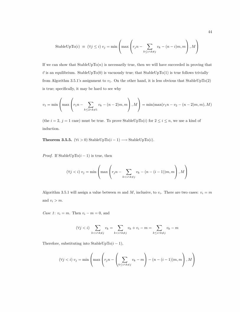
44

StableUpTo(i) ≡ (∀j ≤ i) vj = min

max

rjn−∑

k≤i∧k 6=j

vk − (n− i)m, m

, M

If we can show that StableUpTo(n) is necessarily true, then we will have succeeded in proving that

~v is an equilibrium. StableUpTo(0) is vacuously true; that StableUpTo(1) is true follows trivially

from Algorithm 3.5.1’s assignment to v1. On the other hand, it is less obvious that StableUpTo(2)

is true; specifically, it may be hard to see why

v1 = min

max

r1n−∑

k≤2∧k 6=1

vk − (n− 2)m, m

, M

= min(max(r1n− v2 − (n− 2)m, m), M)

(the i = 2, j = 1 case) must be true. To prove StableUpTo(i) for 2 ≤ i ≤ n, we use a kind of

induction.

Theorem 3.5.5. (∀i > 0) StableUpTo(i− 1) −→ StableUpTo(i).

Proof. If StableUpTo(i− 1) is true, then

(∀j < i) vj = min

max

rjn−∑

k<i∧k 6=j

vk − (n− (i− 1))m, m

, M

Algorithm 3.5.1 will assign a value between m and M , inclusive, to vi. There are two cases: vi = m

and vi > m.

Case 1 : vi = m. Then vi −m = 0, and

(∀j < i)∑

k<i∧k 6=j

vk =∑

k<i∧k 6=j

vk + vi −m =∑

k≤i∧k 6=j

vk −m

Therefore, substituting into StableUpTo(i− 1),

(∀j < i) vj = min

max

rjn−

∑

k≤i∧k 6=j

vk −m

− (n− (i− 1))m, m

, M

45

or

(∀j < i) vj = min

max

rjn−∑

k≤i∧k 6=j

vk − (n− i)m, m

, M

Case 2 : vi > m. Applying Lemma 3.5.2, we have

rin ≥∑

k≤i

vk + (n− i)m

It follows that

(∀j < i) rin ≥∑

k≤i∧k 6=j

vk + vj + (n− i)m

Since vi > m, Lemma 3.5.4 tells us that (∀j < i) vj = M , and so

(∀j < i) rin ≥∑

k≤i∧k 6=j

vk + M + (n− i)m

Then, since (∀j < i) rjn ≥ rin,

(∀j < i) rjn ≥∑

k≤i∧k 6=j

vk + M + (n− i)m

or

(∀j < i) rjn−∑

k≤i∧k 6=j

vk − (n− i)m ≥M

It follows that

(∀j < i) min

max

rjn−∑

k≤i∧k 6=j

vk − (n− i)m, m

, M

= M

Again we can use Lemma 3.5.4, (∀j < i) vj = M , and

(∀j < i) min

max

rjn−∑

k≤i∧k 6=j

vk − (n− i)m, m

, M

= vj

46

Conclusion. So, whether vi = m or vi > m,

(∀j < i) vj = min

max

rjn−∑

k≤i∧k 6=j

vk − (n− i)m, m

, M

In addition, Algorithm 3.5.1 guarantees that vi is assigned the value

min(

max(

rin−∑

k<i vk − (n− i)m, m)

, M)

, which equals

min(

max(

rin−∑

k≤i∧k 6=i vk − (n− i)m, m)

, M)

, so

(∀j ≤ i) vj = min

max

rjn−∑

k≤i∧k 6=j

vk − (n− i)m, m

, M

which is precisely StableUpTo(i).

So, for any i, whether vi = m or vi > m, StableUpTo(i− 1) −→ StableUpTo(i).

We are finally ready to prove that an equilibrium always exists.

Theorem 3.5.6. For any ~r, where 0 ≤ ri ≤ 1 for 1 ≤ i ≤ n, the vote vector ~v returned by

Algorithm 3.5.1 satisfies

(∀i) vi = min

max

rin−∑

k 6=i

vk, m

, M

Proof. If ~v is the vector returned by Algorithm 3.5.1, StableUpTo(0) is vacuously true, and so the

truth of (∀i ≤ n) StableUpTo(i) follows from Theorem 3.5.5. In particular, StableUpTo(n) must be

true:

(∀j ≤ n) vj = min

max

rjn−∑

k≤n∧k 6=j

vk − (n− n)m, m

, M

or

(∀j ≤ n) vj = min

max

rjn−∑

k 6=j

vk, m

, M

which is the optimal strategy for all voters. It directly follows that Algorithm 3.5.1, which is

deterministic and always halts, will necessarily find an equilibrium from which no voter i would

choose to change vi using the rational Average strategy.

47

So an equilibrium ~v must always exist for any input ~r and any m ≤ 0 and M ≥ 1.

We now know that, given some sincere-preference vector ~r,

• at most one value φ satisfies Equations 3.8 and 3.9 (Theorem 3.4.1),

• any equilibrium ~v has average vote v satisfying Equations 3.6 and 3.7 (section 3.2.2), and

• at least one equilibrium ~v must exist (Theorem 3.5.6)

and so we can conclude that any φ that satisfies Equations 3.8 and 3.9 must equal the average vote

v at all equilibria ~v.

3.6 Average-Approval-Rating DSV

We have seen that Algorithm 3.5.1, FindEquilibrium, always finds an equilibrium for any

sincere-preference vector ~r. We also know that any equilibrium ~v will have the same average v

(and that 0 ≤ v ≤ 1). It follows that the average at equilibrium is unique and can be defined as a

function:

Algorithm 3.6.1.

AverageAtEquilibrium(~r, m, M):

~v ← FindEquilibrium(~r, m, M)

return v =�

ni=1

vi

n

Even when m < 0 and/or M > 1, AverageAtEquilibrium will return an outcome between 0 and 1.

In fact, the outcome returned will be within the range defined by the input vector of cardinal

preferences:

Theorem 3.6.2. (∀m ≤ 0, M ≥ 1) min(~r) ≤ AverageAtEquilibrium(~r, m, M) ≤ max(~r).

48

Proof. Say there is some m ≤ 0 and some M ≥ 1 such that

min(~r) > AverageAtEquilibrium(~r, m, M). Then it follows that

(∀i) ri > AverageAtEquilibrium(~r, m, M)

and so

(∀i) ri > v =

∑nj=1 vj

n

where ~v = FindEquilibrium(~r, m, M). According to Equation 3.4,

(∀i) ri > v −→ vi = M

and we can conclude that

(∀i) vi = M

which means that v = M ≥ 1. But (∀i) ri > v, so

(∀i) ri > 1

which contradicts the fact that (∀i) 0 ≤ ri ≤ 1. Therefore there can be no m ≤ 0 and M ≥ 1 such

that min(~r) > AverageAtEquilibrium(~r, m, M).

Now say there is some m ≤ 0 and some M ≥ 1 such that

max(~r) < AverageAtEquilibrium(~r, m, M). Then it follows that

(∀i) ri < AverageAtEquilibrium(~r, m, M)

and so

(∀i) ri < v =

∑nj=1 vj

n

where ~v = FindEquilibrium(~r, m, M). According to Equation 3.5,

(∀i) ri < v −→ vi = m

49

and we can conclude that

(∀i) vi = m

which means that v = m ≤ 0. But (∀i) ri < v, so

(∀i) ri < 0

which contradicts the fact that (∀i) 0 ≤ ri ≤ 1. Therefore there can be no m ≤ 0 and M ≥ 1 such

that max(~r) < AverageAtEquilibrium(~r, m, M).

So there is no m ≤ 0 and M ≥ 1 such that min(~r) > AverageAtEquilibrium(~r, m, M) or

max(~r) < AverageAtEquilibrium(~r, m, M). Therefore it must be that

(∀m ≤ 0, M ≥ 1) min(~r) ≤ AverageAtEquilibrium(~r, m, M) ≤ max(~r)

These bounds are tight; in fact,

(∀M ≥ 1) limm→−∞

AverageAtEquilibrium(~v, m, M) = min(~v)

and

(∀m ≤ 0) limM→+∞

AverageAtEquilibrium(~v, m, M) = max(~v)

3.6.1 A new class of rating systems

The Average and Median protocols necessarily take a vote vector ~v as input—voters’ sincere

preference information cannot be directly and reliably elicited, so ~r is not generally available. If

the Average system is used and voters are rationally strategic (and are allowed to keep changing

their votes until all decide to stand pat), the outcome can reasonably be expected to equal

AverageAtEquilibrium(~r, 0, 1). But instead of using Average on the vote vector ~v and relying on

the voters to use optimally rational strategy when deciding on their votes vi,

AverageAtEquilibrium(~v, 0, 1) can be calculated and taken as the outcome, implicitly and

50

effectively using the DSV [23] framework with Average as the underlying voting protocol. In fact,

we are not limited to AverageAtEquilibrium(~v, 0, 1); we have just seen that

AverageAtEquilibrium(~v, m, M) lies between 0 and 1 for any m ≤ 0 and M ≥ 1 and so can serve as

a rating system as well.

For illustration, we reuse the Videodrome example and assume sincere voters:

~v = [0.4, 0.7, 0.8, 0.8, 0.88]

Suppose we want to take as the outcome of this election not the average vote v or the median vote

v but AverageAtEquilibrium(~v, 0, 1). First we calculate FindEquilibrium(~v, 0, 1), which we have

seen in section 3.2.2 to be

~w = FindEquilibrium(~v, 0, 1) = [0, 0.5, 1, 1, 1]

Then we see that

w =

∑5i=1 wi

5=

0 + 0.5 + 1 + 1 + 1

5= 0.7

giving the outcome as 0.7, which equals neither the Average outcome (v = 0.716) nor the Median

outcome (v = 0.8).

Alternatively, we can let m = −99 and M = 100. Then the equilibrium we find turns out to be

~w = FindEquilibrium(~v,−99, 100) = [−99,−99, 2, 100, 100]

And then

w =

∑5i=1 wi

5=−99 + (−99) + 2 + 100 + 100

5= 0.8

This time the power to determine the outcome fell to voter 3 rather than voter 2, giving the

Median outcome of 0.8. (We will see that if m + M = 1 and M −m is allowed to become large

enough, the resultant outcome will equal the Median outcome.)

It turns out that in neither of these cases will any voter be able to gain from voting insincerely.

For example, if voter 3 in the m = −99, M = 100 case voted anything but 2, the outcome would

51

deviate from the ideal r3 = 0.8; if voter 2 voted anything other than −99, the outcome would be

larger than 0.8, moving farther away from r2 = 0.7. This is no coincidence.

We will now prove that this Average-Approval-Rating (AAR) DSV system has three intuitively

desirable properties: a kind of monotonicity (Theorem 3.6.3), immunity to Average-like strategy

(Theorem 3.6.4) and a general nonmanipulability (Theorem 3.6.5). The first two will imply the

third.

3.6.2 Monotonicity of AAR DSV

First, the monotonicity property: When some input votes are increased and none is decreased, the

outcome never decreases.

Theorem 3.6.3. If ~v = [v1, v2, . . . vn] and ~v′ = [v′1, v′2, . . . v

′n] where (∀i) vi ≤ v′i, then

AverageAtEquilibrium(~v, m, M) ≤ AverageAtEquilibrium(~v′, m, M).

Proof. Equations 3.6 and 3.7 say that

|{i : w < vi}| ≤w −m

M −mn ≤ |{i : w ≤ vi}|

where ~w = FindEquilibrium(~v, m, M).

Therefore, if v = AverageAtEquilibrium(~v, m, M) and v′ = AverageAtEquilibrium(~v′, m, M), it

must be that

|{i : v < vi}| ≤v −m

M −mn ≤ |{i : v ≤ vi}|

and

|{i : v′ < v′i}| ≤v′ −m

M −mn ≤ |{i : v′ ≤ v′i}|

Also, since (∀i) vi ≤ v′i, we have that

(∀i) v ≤ vi −→ v ≤ v′i

52

Assume for now that v > v′. Then

(∀i) v ≤ vi −→ v′ < v′i

and so

{i : v ≤ vi} ⊆ {i : v′ < v′i}

which means that

|{i : v ≤ vi}| ≤ |{i : v′ < v′i}|

But, since v−mM−mn ≤ |{i : v ≤ vi}| and |{i : v′ < v′i}| ≤

v′−mM−mn, it must be true that

v −m

M −mn ≤

v′ −m

M −mn

n is positive, so

v −m

M −m≤

v′ −m

M −m

and M > m, so

v −m ≤ v′ −m

and thus

v ≤ v′

contradicting the assumption that v > v′. Therefore v > v′ must be false, so v ≤ v′.

3.6.3 AAR DSV is immune to Average-style strategy

Another desirable property of AAR DSV is that its outcome is unaffected by voters’ using

Average-style strategy, trying to move the outcome in the desired direction by moving their votes

in that direction.

Theorem 3.6.4. If ~v = [v1, v2, . . . vn] and ~v′ = [v′1, v′2, . . . v

′n] where, for all 1 ≤ i ≤ n,

• v′i ≤ vi if AverageAtEquilibrium(~v, m, M) > vi

53

• v′i = vi if AverageAtEquilibrium(~v, m, M) = vi

• v′i ≥ vi if AverageAtEquilibrium(~v, m, M) < vi

then AverageAtEquilibrium(~v′, m, M) = AverageAtEquilibrium(~v, m, M).

Proof. From the definition of ~v′, we have that

(∀i) v > vi −→ v′i ≤ vi

(∀i) v = vi −→ v′i = vi

(∀i) v < vi −→ v′i ≥ vi

where v = AverageAtEquilibrium(~v, m, M). These respectively imply that

(∀i) v > vi −→ v > v′i (3.10)

(∀i) v = vi −→ v = v′i (3.11)

(∀i) v < vi −→ v < v′i (3.12)

From 3.10 and 3.11 we can see that

(∀i) v ≥ vi −→ v ≥ v′i

Combining the contrapositive of this result with 3.12 gives

(∀i) v < vi ←→ v < v′i

which means that

{i : v < vi} = {i : v < v′i}

54

Since v = AverageAtEquilibrium(~v, m, M), Equation 3.6 tells us that

|{i : v < vi}| ≤v −m

M −mn

and so we can conclude that

|{i : v < v′i}| ≤

v −m

M −mn

Similarly, from 3.11 and 3.12 we can see that

(∀i) v ≤ vi −→ v ≤ v′i

Combining this result with the contrapositive of 3.10 gives

(∀i) v ≤ vi ←→ v ≤ v′i

which means that

{i : v ≤ vi} = {i : v ≤ v′i}

Since v = AverageAtEquilibrium(~v, m, M), Equation 3.7 tells us that

v −m

M −mn ≤ |{i : v ≤ vi}|

and so we can conclude that

v −m

M −mn ≤ |{i : v ≤ v′

i}|

Now we have that

|{i : v < v′i}| ≤

v −m

M −mn ≤ |{i : v ≤ v′

i}|

and, if v′ = AverageAtEquilibrium(~v′, m, M), then v′ satisfies

|{i : v′ < v′i}| ≤v′ −m

M −mn ≤ |{i : v′ ≤ v′i}|

55

Finally, by Theorem 3.4.1, v = v′, and so

AverageAtEquilibrium(~v, m, M) = AverageAtEquilibrium(~v′, m, M).

3.6.4 AAR DSV never rewards insincerity

For any voting system, it is desirable to show that a voter can never gain a better outcome by

voting insincerely than by voting sincerely, however sincerity is defined. It turns out that, when

AverageAtEquilibrium(~v, m, M) is selected as the outcome, no voter i can gain an outcome closer

to the ideal ri by voting vi 6= ri instead of vi = ri, guaranteeing a strong nonmanipulability

property to AAR DSV:

Theorem 3.6.5. If ~v = [v1, v2, . . . vn] where v1 = r1 and ~v′ = [v′1, v′2, . . . v

′n] where v′

1 6= r1 and

(∀i > 1) v′i = vi, then

|AverageAtEquilibrium(~v, m, M)− r1| ≤ |AverageAtEquilibrium(~v′, m, M)− r1|.

Proof. Abbreviating AverageAtEquilibrium(~v, m, M) as v and AverageAtEquilibrium(~v ′, m, M) as

v′, if v = r1, then |v − r1| = 0, and so then we can conclude immediately that

|v − r1| ≤ |v′ − r1|

On the other hand, it may be that v 6= r1. Since it is also true that v′1 6= r1, there are now four

cases to consider:

1. v > r1 and v′1 > r1

2. v > r1 and v′1 < r1

3. v < r1 and v′1 < r1

4. v < r1 and v′1 > r1

Cases 2 and 4 might be said to represent reasonable attempts at effective strategy, while cases 1

and 3 entail insincere voting in the “wrong” direction. Considering them in order:

56

Case 1 : v > r1 and v′1 > r1. Then, since v1 = r1, v′1 > v1; since (∀i > 1) v′i = vi,

(∀i) vi ≤ v′i

and so Theorem 3.6.3 allows us to conclude that

v = AverageAtEquilibrium(~v, m, M) ≤ AverageAtEquilibrium(~v′, m, M) = v′

which means

v − r1 ≤ v′ − r1

We know that v > r1, and v′ > r1 since v ≤ v′, so v − r1 and v′ − r1 are both positive. Thus

|v − r1| ≤ |v′ − r1|

Case 2 : v > r1 and v′1 < r1. Then, since v1 = r1, v > v1 and v′1 < v1. We also know that

(∀i > 1) v′i = vi, so we can use Theorem 3.6.4 to get

v = v′

and it immediately follows that

|v − r1| ≤ |v′ − r1|

Case 3 : v < r1 and v′1 < r1. Then, since v1 = r1, v′1 < v1; since (∀i > 1) v′i = vi,

(∀i) vi ≥ v′i

and so Theorem 3.6.3 allows us to conclude that

v = AverageAtEquilibrium(~v, m, M) ≥ AverageAtEquilibrium(~v′, m, M) = v′

57

which means

v − r1 ≥ v′ − r1

We know that v < r1, and v′ < r1 since v ≥ v′, so v − r1 and v′ − r1 are both negative. Thus

|v − r1| ≤ |v′ − r1|

Case 4 : v < r1 and v′1 > r1. Then, since v1 = r1, v < v1 and v′1 > v1. We also know that

(∀i > 1) v′i = vi, so we can use Theorem 3.6.4 to get

v = v′

and it immediately follows that

|v − r1| ≤ |v′ − r1|

Conclusion. In each case we have found |v− r1| ≤ |v′ − r1| to hold. The cases are exhaustive, so we

can conclude that

|AverageAtEquilibrium(~v, m, M)− r1| ≤ |AverageAtEquilibrium(~v′, m, M)− r1|

So insincere voters under these AAR DSV systems cannot move the outcome closer to ideal.

However, it should be mentioned that a nonmanipulable rating system cannot be easily generalized

to give nonmanipulable single-winner voting protocols. For example, while it is always rational to

vote sincerely when using Median aggregation, the “majority judgement” protocol of Balinski and

Laraki [6] (under which each voter submit cardinal votes over a finite number of discrete

alternatives and the one with the highest median vote wins) can be manipulated by voting

insincerely. For example, say there are three voters and three alternatives, and the votes are

58

A B C

voter 1 0.8 0.7 0.1

voter 2 0.6 0.2 0.4

voter 3 0 0.9 0.3

A’s median vote is 0.6, B’s is 0.7 and C’s is 0.3, so B wins. But if voter 1 gave B an insincere vote

of 0.5 instead, thus lowering B’s median vote to 0.5, A would win and voter 1 would benefit.

3.7 A simpler AAR DSV algorithm

It is possible to find a quicker, more direct way of calculating AverageAtEquilibrium(~v, m, M)

given a vector ~v. One promising approach is to use the property

|{i : φ < vi}| ≤φ−m

M −mn ≤ |{i : φ ≤ vi}|

We know that, given ~v, this property is true for exactly one value φ, which is equal to

AverageAtEquilibrium(~v, m, M). The problem is that φ may be any number between 0 and 1;

testing every 0 ≤ φ ≤ 1 individually is impossible.

Happily, it turns out that testing a finite number of possibilities for φ is sufficient to guarantee

finding one that satisfies the above property. In particular, AverageAtEquilibrium(~v, m, M) is

always equal to either vi for some 1 ≤ i ≤ n or m + M−mn i for some i ∈ � , 0 ≤ i ≤ n.

Theorem 3.7.1.

(∃i ∈ � ) AverageAtEquilibrium(~v, m, M) = vi ∨ AverageAtEquilibrium(~v, m, M) = m + M−mn i.

Proof. Recall that, given some vote vector ~v,

AverageAtEquilibrium(~v, m, M) =

∑

i FindEquilibrium(~v, m, M)i

n

Define ~w ≡ FindEquilibrium(~v, m, M), the vector that results when ~v is treated as the voters’

sincere preferences and optimal Average strategy is applied on behalf of all voters until an

59

equilibrium is reached. We now proceed in two cases: Either there is some wi such that

m < wi < M or there is none.

Case 1. (∃i) m < wi < M . Take i to be any value such that m < wi < M . Since

~w = FindEquilibrium(~v, m, M), we know by Theorem 3.5.6 that

(∀j) wj = min

max

vjn−∑

k 6=j

wk, m

, M

and, in particular for i,

wi = min

max

vin−∑

k 6=i

wk , m

, M

Since m < wi < M ,

wi = vin−∑

k 6=i

wk

and therefore

vin = wi +∑

k 6=i

wk =∑

k

wk

and

vi =

∑

k wk

n= AverageAtEquilibrium(~v, m, M)

It follows that (∃i) vi = AverageAtEquilibrium(~v, m, M). This case illustrates that any voter at

equilibrium not voting at one of the extremes must have realized his or her ideal outcome.

Case 2. (∀i) wi = m ∨ wi = M . Then∑

k wk must equal jM + (n− j)m = nm + j(M −m) for

integer j = |{i : wi = M}|. So we have

AverageAtEquilibrium(~v, m, M) =

∑

k wk

n=

nm + j(M −m)

n= m +

M −m

nj

and it follows that (∃i ∈ � ) AverageAtEquilibrium(~v, m, M) = m + M−mn i.

Conclusion. These two cases are exhaustive. Therefore,

(∃i ∈ � ) AverageAtEquilibrium(~v, m, M) = vi ∨ AverageAtEquilibrium(~v, m, M) = m +M −m

ni

60

This fact would seem to motivate a direct and efficient algorithm for computing

AverageAtEquilibrium(~v, m, M). First, take O(n log n) time to sort ~v so that v1 ≥ v2 ≥ . . . ≥ vn.

Then binary searches can be used to test each vi value and each M−mn i value. For each potential

solution φ, if

φ−m

M −mn > |{i : φ ≤ vi}|

then we can rule out φ and every value greater than φ; if

|{i : φ < vi}| >φ−m

M −mn

then we can rule out φ and every value less than φ. Each of these tests runs in O(n) time, so the

binary searches will finish and the correct outcome will be found (as Theorem 3.7.1 guarantees) in

O(n log n) time.

Another efficient approach is to streamline Algorithm 3.6.1 directly:

AverageAtEquilibrium(~v, m, M):

sort ~v so that (∀i ≤ j) vi ≥ vj

for i = 1 to n do

wi ← min(

max(

vin−∑

k i and applies the optimal strategy

function for the ith voter:

Algorithm 3.7.2.



for i = 1 to n do

wi ← m

for i = 1 to n do

wi ← min(

max(

vin−∑

k 6=i wk, m)

, M)

61

return w =�

ni=1

wi

n

Instead of calculating∑

k 6=i wk freshly each time, we can easily keep track of wsum =∑

k wk and

subtract wi = m from it. For the first loop iteration wsum is equal to∑

k m = nm, and from the ith

to the (i + 1)th iteration it increases by wi −m, as the new value of wi replaces the old value, m:

Algorithm 3.7.3.



wsum ← nm

for i = 1 to n do

wi ← min (max (vin− wsum + m, m) , M)

wsum ← wsum + wi −m

return w =� n

i=1wi

n

Now we can get rid of ~w entirely:

Algorithm 3.7.4.



wsum ← nm

for i = 1 to n do

wsum ← wsum + min (max (vin− wsum , 0) , M −m)

return wsum

n

The sorting step can be done in O(n log n) time; each wsum update takes constant time, so

everything after the sorting step finishes in O(n) time.

62

3.8 Parameterizing AAR DSV

Given a vote vector ~v, we have seen that the outcome v = AverageAtEquilibrium(~v, 0, 1) of “pure”

AAR DSV, which is DSV applied to the original [0, 1]-Average system, satisfies the property

|{i : v < vi}| ≤ vn ≤ |{i : v ≤ vi}|

We also know that the order-statistic outcome bv (the generalization of Median from section 3.1.3),

for constant 0 ≤ b ≤ 1, satisfies

|{i : bv < vi}| ≤ bn ≤ |{i : bv ≤ vi}|

This looks like a job for interpolation! We define a new parameter a that varies between 0 (giving

bv) and 1 (giving AverageAtEquilibrium(~v, 0, 1)). The generalized outcome Φa,b(~v) then will satisfy

|{i : Φa,b(~v) < vi}| ≤ (aΦa,b(~v) + (1− a)b)n ≤ |{i : Φa,b(~v) ≤ vi}| (3.13)

and we have already found exactly such a function. We know that

|{i : v < vi}| ≤v −m

M −mn ≤ |{i : v ≤ vi}|

where v = AverageAtEquilibrium(~v, m, M). So if

Φa,b(~v)−m

M −m= aΦa,b(~v) + (1− a)b

where a = 1M−m , b = m

1−M+m , m = b− ba and M = b + 1−b

a , then we can define

Φa,b(~v) ≡ limx→a+

AverageAtEquilibrium

(

~v, b−b

x, b +

1− b

x

)

and Φa,b(~v) will satisfy Equation 3.13. (The limit is needed for the a = 0 case; as a approaches 0,

Φa,b(~v) approaches the bv outcome defined in section 3.1.3.) In fact, a value φ satisfies

|{i : φ < vi}| ≤ (aφ + (1− a)b)n ≤ |{i : φ ≤ vi}|

63

if and only if φ = Φa,b(~v), as we showed in section 3.5.

Theorem 3.8.1. (∀a, b) min(~v) ≤ Φa,b(~v) ≤ max(~v).

Proof. Whenever 0 ≤ a, b ≤ 1, it is true that

ab ≤ b

and so

limx→a+

b−b

x≤ 0 (3.14)

It also must be that a− 1 ≤ 0 and b− 1 ≤ 0, so

(a− 1)(b− 1) = ab− a− b + 1 ≥ 0

and

ab + 1− b ≥ a

which means

limx→a+

b +1− b

x≥ 1 (3.15)

Theorem 3.6.2 says that

(∀m ≤ 0, M ≥ 1) min(~v) ≤ AverageAtEquilibrium(~v, m, M) ≤ max(~v)

Given this and Equations 3.14 and 3.15, it follows that

(∀a, b) min(~v) ≤ limx→a+

AverageAtEquilibrium

(

~v, b−b

x, b +

1− b

x

)

≤ max(~v)

By definition of the Φa,b function, we can conclude that

(∀a, b) min(~v) ≤ Φa,b(~v) ≤ max(~v)

64

Therefore any Φ function’s output can be neither higher than all inputs nor lower than all inputs.

In particular, if (∀i) vi = ω, then (∀a, b) Φa,b(~v) = ω, so any Φ function satisfies an intuitively

appealing unanimity property: when all voters agree, the outcome agrees with them.

3.9 Evaluation of AAR DSV systems

Any system that uses the outcome function Φa,b(~v) where 0 ≤ a ≤ 1 and 0 ≤ b ≤ 1 has the

property that no voter can gain by voting insincerely. But it does not follow that any values of a

and b give equally desirable outcomes.

One approach to evaluating this continuous range of nonmanipulable systems is to take the

Average system as a benchmark and determine which Φa,b function comes nearest, on average, to

giving the Average outcome. Given a vote vector ~v, we can calculate the Average outcome v and

the outcome Φa,b(~v) for many a, b combinations. For any particular a and b, we can calculate the

squared error from v:

SEa,b(~v) = (Φa,b(~v)− v)2

If V = {~v1, ~v2, ~v3 . . . ~vN} is a vector of N vote vectors, then we can find the root-mean-squared

error from Average, weighted by the number of ratings in each vote vector ~vi:

RMSEa,b(V) =

√

√

√

√

∑Ni=1|~vi| · SEa,b(~vi)∑N

i=1|~vi|

Given some “training” vector V of vote vectors, we would like to choose a and b to minimize

RMSEa,b(V).

This approach requires a concrete source of vote-vector data or a distribution for generating such.

The website Metacritic [1] offers ideal data for our purposes: Reviews for over 4000 films (plus

many books, music albums, video games, etc.) are summarized into ratings between 0 and 100.

For example, one film1 has the seven ratings 70, 70, 80, 80, 88, 88 and 100, which are easily

1The 1978 film Animal House.

65

converted into the vote vector

~v = [0.7, 0.7, 0.8, 0.8, 0.88, 0.88, 1]

Converting all films on Metacritic the same way gives us a large vector V of vote vectors.2

Since there are two parameters, a and b, it is somewhat impractical to try all combinations. But it

may be desired to fix b = 0.5 to ensure a kind of symmetry: If (∀i) v′i = 1− vi, then

(∀a) Φa,0.5(~v′) = 1− Φa,0.5(~v), so electorates that prefer low and high outcomes are treated

symmetrically. Fixing b = 0.5 and trying all 10001 evenly spaced values of a, we find that

a = 0.3240 (Figure 3.1) gives the minimum RMSE for the Metacritic data.

Figure 3.1: RMSE, varying a and fixing b = 0.5000

0.032

0.034

0.036

0.038

0.04

0.042

0.044

0.046

0.048

0.05

0 0.2 0.4 0.6 0.8 1

RMSE

a

Having fixed b = 0.5 and found the value of a that minimizes RMSE (0.3240), we can now fix

a = 0.3240 and find the value of b that minimizes RMSE, then fix b again accordingly and continue

2We use the data for the 4581 films mined from Metacritic on Thursday, 3 April 2008, that had at least threecritics rate them.

66

in a hill-climbing fashion until we find a stable minimum. In practice, the procedure is guaranteed

to halt because the RMSE decreases at each step for which either a or b changes.

Using this procedure on the Metacritic data and testing 10001 evenly spaced values of a or b at

each step, whether we start with a = 0 or with b = 0.5, we find a local RMSE minimum

(approximately 0.03242) at a = 0.3647, b = 0.4820 (Figures 3.2 and 3.3); such a system is

equivalent to running an Average election with rationally optimal voters and allowing votes

between m ≈ −0.8396 and M ≈ 1.9023.

Figure 3.2: RMSE, varying a and fixing b = 0.4820

0.032

0.034

0.036

0.038

0.04

0.042

0.044

0.046

0.048

0.05

0 0.2 0.4 0.6 0.8 1

RMSE

a

It can be seen in Figure 3.4 that Φ0.3647,0.4820(~v) and v do indeed correlate nicely for the

Metacritic data.

To a good approximation, then, the AAR DSV system that comes closest to matching Average

outcomes for the Metacritic data is one with a = 13 and b = 1

2 , which corresponds to allowing votes

between m = −1 and M = 2.

67

Figure 3.3: RMSE, fixing a = 0.3647 and varying b

0.02

0.04

0.06

0.08

0.1

0.12

0.14

0.16

0 0.2 0.4 0.6 0.8 1

RMSE

b

3.10 Generalizations to more dimensions

What if the votes and the outcome are in d-dimensional space, where d > 1 and each dimension is

restricted between 0 and 1 (giving a hypercube)? For example, if the votes are (0.3, 0.3), (0.3, 0.3),

(0.3, 0.7), (0.7, 0.3) and (0.7, 0.7), what should the outcome be? This problem is very similar to

single point estimation, the problem of finding a most “representative” point given a set of points.

The Average system is easily generalized to multiple dimensions by taking the average of each

coordinate, effectively calculating the centroid, the center of mass given a set of unit masses.

(Alternatively, one can imagine attaching Hookean springs of equal spring constants to each fixed

input point, then gluing the other ends of the springs together; the glue point will come to rest at

the centroid.) This generalization is equivalent to finding the point t that minimizes

n∑

i=1

dist(t, vi)2

68

Figure 3.4: Φ0.3647,0.4820(~v) vs. v scatterplot

0

0.2

0.4

0.6

0.8

1

0 0.2 0.4 0.6 0.8 1

Φ0.3647,0.4820

outcome

Average outcome

where dist(t, vi) =(

∑dj=1(tj − vij)

2)1/2

, the Euclidean distance between t and vi (and the `2

norm of the vector t− vi). (We must now conceptually allow all real numbers, not just rationals.)

The resulting system is rotationally invariant and is equivalent to conducting d separate and

independent Average elections, and the results above for strategic behavior under the

one-dimensional Average system apply to the “election” for each coordinate. In particular,

conducting a d-dimensional Average DSV election is equivalent to conducting d parallel

one-dimensional Average DSV elections, and so gives a nonmanipulable system.

Generalizing Median to multiple dimensions by finding the median of each coordinate also results

in a nonmanipulable system, but, unlike in the Average case, the result is not rotationally

invariant (consider the points (0, 0), (0, 1) and (1, 0), and then rotate them 45 degrees). But these

are not the only ways to generalize the above one-dimensional systems.

69

First, the one-dimensional space between 0 and 1 (or −1 and 1) can be generalized in other ways

than into hypercubes. For example, the d-dimensional space could be the zero-centered

d-dimensional sphere of radius 1 (for example, {(x, y) ∈ � 2 : x2 + y2 ≤ 1}), and each voter can be

assumed to prefer points with smaller Euclidean distance to his or her ideal point to those farther

from it. Or it could be the d-dimensional surface of the (d + 1)-dimensional sphere of radius 1 (for

example, {(x, y) ∈ � 2 : x2 + y2 = 1}). Perhaps even more interestingly, the outcome space could be

the d-dimensional simplex (for example, {(x, y, z) ∈ � 3 : x + y + z = 1}), which could describe the

division of a limited resource among several uses (such as a committee allocating a fixed sum

among budget items). Applying DSV to these problems may be addressed in future work.

Second, the Median system itself can be generalized in other interesting ways besides applying it

independently to each coordinate. An alternative, and arguably superior, generalization of the

Median system is found by finding the point t that minimizes

n∑

i=1

dist(t, vi)

t is known as the Fermat–Weber point [58, 17]. The resulting system is rotationally invariant,

unlike the median-in-each-dimension system. When d > 1, unlike in the one-dimensional case, it

usually has a single optimum point even when n is even (the only exception is an even number of

collinear points). Unfortunately, there is no computationally feasible exact algorithm to calculate

the Fermat–Weber point in general [5], but numerical approximation is quite easy [56, 11].

The Fermat–Weber point does not change when a point vi is moved farther away from t in the

direction of the vector ~tvi [54], so, in a sense, direction matters but not distance. Because of this

property, a naıve Average-style strategy for manipulating this Fermat–Weber system fails, and any

successful manipulation would have to move a sincere vote in some other direction.

Unfortunately, an insincere voter can indeed manipulate the Fermat–Weber point to move closer to

his or her ideal outcome. Consider the square outcome space {(x, y) ∈ � 2 : 0 ≤ x, y ≤ 1}. If there

are four voters whose ideal outcomes are (0.4, 0), (0.4, 1), (0.6, 0) and (0.6, 1), and they all vote

sincerely, then the Fermat–Weber point is (0.5, 0.5). But then the fourth voter can insincerely vote

(0.4, 1), giving a Fermat–Weber point of (0.4, 1), which is closer by Euclidean distance to the ideal

(0.6, 1) than is the previous outcome (0.5, 0.5).

70



1. Described a rational voter’s optimal strategy for Average aggregation.

2. Proved that at least one equilibrium will exist when all Average voters are optimally

strategic.

3. Proved that all such equilibria will have the same Average outcome.

4. Defined a large new class of AAR DSV systems and showed that they are all immune to

manipulation by insincere voters.

5. Provided an efficient algorithm to compute any AAR DSV outcome.

6. Used real-world data to choose an AAR DSV system that comes closest to matching Average

outcomes over those data.

7. Showed that using the Fermat–Weber point as the outcome in a multi-dimensional space can

be manipulated by insincere voters.

71

Chapter 4

Comparing Approval Strategies for

DSV

DSV systems have been considered for plurality elections with the following goals in mind. First, it

is known that voters will behave strategically, in that they will vote an insincere ballot if they are

convinced a better outcome can be obtained. DSV systems attempt to distill the sincere cardinal

preferences of a voter into the best possible strategic behavior for that voter. One obvious benefit

is that the voter is motivated to provide sincere cardinal preferences, secure in the knowledge that

his or her strategy will vote effectively according to those preferences. If DSV systems can derive

provably best possible strategic voting behavior from those preferences, then providing other than

sincere cardinal preferences would not be in the best interest of the voter. Second, reasoning about

the best possible strategic behavior may be difficult and well beyond the means of some voters. A

DSV system has the potential of affording the same advantages to all voters, so that no voter has

disproportionate power in an election.

So a goal of DSV systems was to allow greater expression from a voter while providing that voter

the best possible thinking in an election situation.

The above factors are also compelling arguments for elections using approval voting. Approval

ballots are more expressive than plurality ballots, since favor can be expressed for multiple

72

alternatives; in particular, a voter can approve both favorite and compromise alternatives. Thus, it

may be the case that an effective approval ballot is, in some sense, more sincere than a plurality

ballot of equal effectiveness. That is, there exists a (weakly, at least) sincere approval ballot that

has the same or greater effectiveness as a correspondingly effective but insincere plurality ballot.

But Cranor’s and Cytron’s [23] approach to plurality strategy cannot be trivially extended to

approval voting; that is, using their strategy to find the optimal plurality ballot and then

converting it into an approval ballot simply by adding all alternatives preferred to the one already

approved will not necessarily result in an optimal approval ballot. The problem is not simply

finding the optimal alternative for which to vote but finding the optimal cutoff point between

approved and disapproved alternatives; in other words, instead of maximizing a measure of

effectiveness, a natural threshold above which approval is optimal must be found.

For example, if a voter prefers A to B to C, and C is judged to have far and away the best chance

of winning with B the least likely to win, then the Cranor/Cytron approach to plurality strategy

would recommend voting for A. Extending that plurality ballot trivially to an approval ballot by

also approving all alternatives preferred to A results in approving only A, but it may well be that

approving both A and B will give the voter a higher expected utility of the outcome. Indeed,

“strategy A”, presented in section 4.2 and later seen to be optimal under certain conditions

(sections 4.4.6 and 4.5.1), would recommend approving both A and B.

Given extant work on DSV systems and on approval voting, it seems natural to examine the extent

to which DSV systems can be used beneficially in approval elections. The following questions arise:

1. Is there a rationally optimal strategy for approval elections that is suitable under the same

assumptions used for plurality elections (i.e., Cranor/Cytron DSV pivot-probability

computations and equations from social-choice literature concerning utilities)?

2. Under a wider set of assumptions, how do various approval voting strategies compare in

terms of their cost, their effectiveness and their ability to elicit sincere cardinal preferences

from voters?

73

In this chapter we begin the work of examining the above issues. A long-term goal of work in this

area would be to establish strategies that work as well as any voter could in an approval election.

While we may not fully reach that goal in this work, we propose methodologies for evaluating the

effectiveness of an approval strategy and methods for comparing strategies.

4.1 The space of approval ballots

One might assume strategizing in an approval election to be more difficult than in a plurality

election, since the number of allowed ballots is exponential in the number of alternatives rather

than linear. But rarely does it make sense to vote an approval ballot that is not even weakly sincere

by the definition in chapter 1, and in fact it never makes sense when all other ballots are known

and fixed. More importantly from a DSV point of view, as we saw in section 1.4, only weakly

sincere ballots make sense given only the information in an election state as set out in chapter 1.

There are only k + 1 possible weakly sincere approval ballots over k alternatives (and fewer if

abstention is ruled out or if the voter’s cardinal preferences impose only a partial order on the

alternatives). So only O(k) ballots need to be considered for any one voter.

4.2 A new declared strategy for approval voting

Somewhat similar to approval strategy T (Figure 1.3) is strategy A [35], which essentially (when

preferences and election state are tie-free) approves all alternatives preferred to the currently

leading alternative, including that leading alternative if preferred to the currently second-place

alternative. In other words, it places an approval cutoff next to the current leader on the side of

the current second-placer. More precisely and generally, we define strategy A in Figure 4.1.

Notice that when there are no ties in the election state or in the voter’s cardinal preferences,

strategy A effectively approves alternative i if and only if pi ≥ p1 when p1 > p2 and pi > p1 when

p1 < p2.

74

Figure 4.1: Approval strategy A



– find smallest y such that p(v, i) · |Topy(r)| 6= PSumy(v, r) (y = k if none)

– approve alternative i if and only if p(v, i) · |Topy(r)| > PSumy(v, r)

4.3 Evaluating approval strategies

Our assumption is that all a voter ultimately cares about is the outcome of an election.

Accordingly, perhaps the ideal measure of a particular strategy’s effectiveness is, according to some

distribution of sets of one focal voter’s preferences and other voters’ programs, the weighted

average of the values of the outcomes that result when the focal voter uses that strategy. The

difficulty of using such an approach to strategy evaluation is chiefly computational, but the

approach also relies on finding such a distribution that is compellingly realistic.

4.3.1 Evaluating election states directly

Instead of trying to evaluate a strategy based on the eventual outcomes that obtain when it is

used, then, one could simply find a way to evaluate the election states that immediately obtain. If,

given a particular election state and set of preferences, one strategy produces a ballot that leads to

an election state judged to be better by some measure than the election state found by another

strategy, we could judge the first strategy superior to the second in that isolated case.

To illustrate this approach, here’s one relatively simple way to evaluate a given election state:

Chapter 6 of Merrill [38] inspires a way to estimate the expected value of the eventual election

result by using only each alternative’s current vote total. Wi, the probability of alternative i’s

winning, is estimated at Wi =sx

i�kj=1

sxj

where si is alternative i’s current vote total (alternative i’s

entry in the election state) and x is some constant greater than 1; Merrill (somewhat arbitrarily)

suggests using x = 2.1 Wi values estimated in this way can then be used to calculate an estimated

1Relatively speaking, using a smaller x spreads out the winning probability among the alternatives; using a largerx gives a relatively higher winning probability to the current leaders. Therefore it might make sense to vary x byincreasing it as the election progresses, say by doubling it after each round.

75

value of the election from a particular voter’s point of view by calculating∑k

i=1 piWi, where pi is

the cardinal preference that voter gives to alternative i.

For example, suppose the voter that submitted the program that executes next in a

three-alternative approval DSV election rated the alternatives[

1, 23 , 0]

, and the current election

state is [14, 5, 10]. Now the program must decide whether to vote [1, 0, 0] or [1, 1, 0], essentially

choosing between the election states [15, 5, 10] (if only the first alternative is approved) and

[15, 6, 10] (if the first two are approved).

Strategies T and J, described in chapter 1, disagree on the best ballot to cast in this situation; T

recommends [1, 0, 0] and J recommends [1, 1, 0]. So, according to this election-state-evaluation

approach, T makes the right choice if [15, 5, 10] is estimated to have a superior value to [15, 6, 10]

and J makes the right choice if the opposite is true.

Calculating the estimated value of each election state is straightforward. For [15, 5, 10], the

estimated probabilites of winning (assuming x = 2) are

[

152, 52, 102]

152 + 52 + 102=

[

9

14,

1

14,

4

14

]

≈ [0.643, 0.071, 0.286]

and so the estimated value of this election state is2

[

9

14,

1

14,

4

14

]

·

[

1,2

3, 0

]

=9

14+

1

21=

29

42≈ 0.6905

For [15, 6, 10], the estimated probabilites of winning are

[

152, 62, 102]

152 + 62 + 102=

[

225

361,

36

361,100

361

]

≈ [0.623, 0.100, 0.277]

and so the estimated value of this election state is

[

225

361,

36

361,100

361

]

·

[

1,2

3, 0

]

=225

361+

24

361=

249

361≈ 0.6898

2The symbol · denotes vector dot product: [a1, a2, . . . an] · [b1, b2, . . . bn] = [a1b1, a2b2, . . . anbn] = � ni=1 aibi.

76

Since 0.6905 > 0.6898, [15, 5, 10] is judged to be a better election state for the voter than [15, 6, 10]

and so strategy T is the superior performer in this specific case.

A similar example situation shows that strategy T does not always perform better for a voter than

strategy J by this measure. Suppose the next program’s voter again rates the alternatives[

1, 23 , 0]

,

but now the current election state is [9, 5, 15]. This time, again, strategy T recommends the ballot

[1, 0, 0], leading to [10, 5, 15], and J recommends [1, 1, 0], leading to [10, 6, 15]. For [10, 5, 15], the

estimated probabilites of winning, again assuming x = 2, are

[

102, 52, 152]

102 + 52 + 152=

[

4

14,

1

14,

9

14

]

≈ [0.286, 0.071, 0.643]


[

4

14,

1

14,

9

14

]

·

[

1,2

3, 0

]

=4

14+

1

21=

1

3≈ 0.3333

For [10, 6, 15], the estimated probabilites of winning are

[

102, 62, 152]

102 + 62 + 152=

[

100

361,

36

361,225

361

]

≈ [0.277, 0.100, 0.623]


[

100

361,

36

361,225

361

]

·

[

1,2

3, 0

]

=100

361+

24

361=

124

361≈ 0.3435

Since 0.3435 > 0.3333, [10, 6, 15] is judged to be a better election state for the voter than [10, 5, 15]

and so strategy J now performs better in this case. Therefore, according to this election-state

measure, neither strategy T nor J outperforms the other in every possible situation; both

sometimes give inferior ballot recommendations.

This method of estimating alternatives’ eventual winning probabilities by magnifying the vote

totals of leading alternatives illustrates one way to evaluate strategies by evaluating election states.

It essentially takes rules of thumb, which have been described in the literature and are easy to

describe in English, and evaluates them according to a standard which has appeared in the

77

literature and is mathematically precise and easily motivated and parameterized. But, still, it may

seem somewhat arbitrary, not directly taking into account a probability distribution of future

ballots. More compelling election-state-evaluation approaches are possible.

4.3.2 Evaluating election states by looking ahead

When a program is run during a DSV election, it has information on the ballots previously cast

but cannot predict ballots to come with certainty. Any ballot that it chooses may turn out to have

been the most effective one and it may not. The best that can be hoped for, therefore, is to

maximize the expected value of the election for its voter, and to do so requires the program to

make an assumption about the probabilities of the various possible outcomes.

Say an approval DSV election is run in ballot-by-ballot mode with only one round. A particular

voter’s program is about to be run; the ballot vector contains the ballots of those voters whose

programs have already been run. The current program has no information about the ballots to

come. One could imagine the situation as a large decision tree where each node corresponds to a

set of voted ballots and a resulting election state. Each node’s children are the states reachable

from it by voting some specific ballot. The root of the tree is the current election state, and the

leaves are those election states that result when all ballots have been cast and a winner can be

crowned. The question then becomes, How likely is each leaf to be the one corresponding to the

outcome eventually reached?3 Knowing these probabilities, the program can calculate the expected

value of the election for its voter for each possible ballot by weighting the outcomes according to

their assumed probabilities of occurring and vote the ballot that maximizes that expected value.

There are at least two reasonable ways to estimate the leaf outcome probabilities. One, the

agnostic approach, is to assume that at each node in the tree, the relevant program chooses each

possible ballot with equal likelihood. All leaf outcomes reachable from the root node are therefore

assumed to be equally likely to obtain. Another, the statistical approach, is to consider the ballots

seen so far as a representative sample of the final set of ballots and assume that the probability of

each future ballot approving an alternative is equal to the proportion of ballots seen so far that

3This question, in which we know a set of intermediate vote totals and ask about likely eventual totals, is muchlike the inverse of the “ballot problem” [50], in which we know the eventual vote total for each alternative and askabout intermediate vote totals as the ballots are counted one by one.

78

approve that alternative. (These two approaches could be combined; for example, programs run

early in the DSV round might assume all outcomes to be relatively equally probable while those

coming later in the round might tend toward the statistical-sample approach.)

Once an expected value of the election can be computed for each possible ballot, they can be

directly compared. By this standard, a strategy is better than another in a specific instance if it

chooses a ballot with a higher expected value of the election. Similarly, a strategy

election-state-dominates another if it never chooses a ballot that leads to an election state with a

lower expected value of the election than the other, no matter the current election state.

As an example, consider a single-round approval DSV election in ballot-by-ballot mode with three

alternatives and 26 voters. Twenty-four of those voters’ programs have already executed and voted

their ballots, resulting in the election state [10, 12, 12]; therefore 512 of those voters approved a1 and

12 of them approved each of a2 and a3. The penultimate voter’s cardinal preferences are [1, 2

5 , 0], so

his or her program needs only to consider the ballots [1, 0, 0] and [1, 1, 0]. If [1, 0, 0] is chosen, the

new election state will be [11, 12, 12], and the winner of the election will depend on the ballot voted

by the ultimate voter’s program. There are eight possibilities:

ultimate voter’s resulting final value of winner(s) to estimated probability expected

ballot election state penultimate voter of occurrence value

[0, 0, 0] [11, 12, 12] 15 = 0.2 7

48 ≈ 0.146 7240 ≈ 0.029

[0, 0, 1] [11, 12, 13] 0 748 ≈ 0.146 0

[0, 1, 0] [11, 13, 12] 25 = 0.4 7

48 ≈ 0.146 7120 ≈ 0.058

[0, 1, 1] [11, 13, 13] 15 = 0.2 7

48 ≈ 0.146 7240 ≈ 0.029

[1, 0, 0] [12, 12, 12] 715 ≈ 0.467 5

48 ≈ 0.104 7144 ≈ 0.049

[1, 0, 1] [12, 12, 13] 0 548 ≈ 0.104 0

[1, 1, 0] [12, 13, 12] 25 = 0.4 5

48 ≈ 0.104 124 ≈ 0.042

[1, 1, 1] [12, 13, 13] 15 = 0.2 5

48 ≈ 0.104 148 ≈ 0.021

total expected value: 41180 ≈ 0.2278

When two or more alternatives tie for the win, the tie is assumed to be broken with equal

probability; for example, when the final election state is [11, 13, 13], a2 and a3 tie for the win and

so the penultimate voter’s expected value of this outcome is 12 ·

25 + 1

2 · 0 = 15 . The estimated

79

probability of each of the ultimate voter’s ballots is calculated by assuming that the ultimate voter

approves ai with probability equal to the proportion of ai’s approval among ballots seen so far. So

the probability of the ultimate voter’s ballot being [0, 1, 0] equals 712 (the proportion of ballots so

far that did not approve a1) times 12 (the proportion of ballots so far that did approve a2) times 1

2

(the proportion of ballots so far that did not approve a3). The total of the product column is the

estimated value of the final outcome from the penultimate voter’s point of view.

On the other hand, if the penultimate voter’s program chooses the ballot [1, 1, 0], the new election

state will be [11, 13, 12], and the possibilities become

ultimate voter’s resulting final value of winner(s) to estimated probability expected

ballot election state penultimate voter of occurrence value

[0, 0, 0] [11, 13, 12] 25 = 0.4 7

48 ≈ 0.146 7120 ≈ 0.058

[0, 0, 1] [11, 13, 13] 15 = 0.2 7

48 ≈ 0.146 7240 ≈ 0.029

[0, 1, 0] [11, 14, 12] 25 = 0.4 7

48 ≈ 0.146 7120 ≈ 0.058

[0, 1, 1] [11, 14, 13] 25 = 0.4 7

48 ≈ 0.146 7120 ≈ 0.058

[1, 0, 0] [12, 13, 12] 25 = 0.4 5

48 ≈ 0.104 124 ≈ 0.042

[1, 0, 1] [12, 13, 13] 15 = 0.2 5

48 ≈ 0.104 148 ≈ 0.021

[1, 1, 0] [12, 14, 12] 25 = 0.4 5

48 ≈ 0.104 124 ≈ 0.042

[1, 1, 1] [12, 14, 13] 25 = 0.4 5

48 ≈ 0.104 124 ≈ 0.042

total expected value: 720 = 0.3500

The penultimate voter’s estimated value of the final outcome is greater when voting [1, 1, 0] than

[1, 0, 0], so in this situation a strategy that recommended [1, 1, 0] would be judged better than one

that recommended [1, 0, 0]. If the first strategy were never similarly judged inferior to the second

strategy for any such situation, then it would be said to election-state-dominate the second.

This branching-probabilities approach to computing the expected value of an election state results

in a very similar distribution of expected vote totals as Cranor’s [22] pivot-probability approach.

But instead of taking the parameter S2 as an estimate of uncertainty, the branching-probabilities

approach requires knowing how many ballots are still to come. This knowledge is possible when

running a single-round ballot-by-ballot DSV election, as was assumed above. However, the same

approach can be used for multi-round and batch DSV elections in at least two ways. First, it could

80

be assumed that the current round is the last one and proceed accordingly. Second, and arguably

more satisfying, the calculation could be carried out while allowing the number of future ballots to

approach infinity—roughly equivalent to having S2 approach zero in the pivot-probability

approach. Note that this approach will in the limit assign to any election state with a clear leading

alternative an expected value equal to the value of that alternative, but one election state will

usually have a larger expected value than another as the number of future ballots is increased, even

if the same alternative leads in both election states.

For example, imagine that the 20th voter in a three-alternative approval DSV election has the

cardinal preferences[

1, 13 , 0]

and is about to vote; the current election state is [9, 6, 13]. The voter’s

declared strategy considers voting either the ballot [1, 0, 0], leading to the election state [10, 6, 13],

or the ballot [1, 1, 0], leading to the election state [10, 7, 13]. When the number of future ballots is

allowed to approach infinity, the expected value of each of the two considered election states

approaches 0, making no distinction between the two. But if it can be shown that the expected

value of [10, 7, 13] is always greater than that of [10, 6, 13] as the number of future ballots

approaches infinity, then, in this case, the ballot [1, 1, 0] could be said to dominate the ballot

[1, 0, 0].

But how can the effectiveness of two different strategies be compared when neither dominates the

other by this measure? One approach would make more assumptions regarding the likelihoods of

all possible election situations and calculate a weighted average of expected election values, but it

may be difficult to make the problem computationally feasible without making extremely

restrictive assumptions.

When neither of two strategies election-state-dominates the other, so that strategy α is better than

strategy β in some situations and β is better than α in others, a new “uberstrategy” can be

created that is superior to both. Simply define strategy αβ as the strategy that, in any particular

situation, uses the election-state metric to decide whether α’s or β’s recommended ballot has a

better expected election result and follow that recommendation. The resulting strategy αβ

necessarily election-state-dominates each of α and β. The computational cost of such a constructed

uberstrategy may, however, be substantial compared to that of the component strategies.

81

4.4 General results using the Merrill election-state metric

We’ve seen some approaches to comparing relative effectiveness of approval strategies in specific

situations, but it may not be obvious how to use these election-state metrics to compare two

strategies against each other in general. Nevertheless, it is possible to prove some relatively general

results using the Merrill election-state metric defined above.

In this section we compare strategies by looking at decisions from one particular focal voter’s point

of view at a time, so the relevant voter v and the current round r can be treated as constants. As a

notational convenience, we use pi to mean p(v, i), the focal voter’s cardinal preference for

alternative i, and si to mean s(i, r − 1), alternative i’s vote total in the current visible election

state.

4.4.1 Comparing strategies A and T in the three-alternative case

A compelling result can be obtained by focusing on elections with three alternatives4 and

comparing strategies A and T. We narrow consideration to situations in which no two alternatives

are tied in the election state (further assuming with no loss of generality that alternative 1 is in the

lead followed by alternative 2 and then alternative 3) and the focal voter has strictly ordered

cardinal preferences.

Theorem 4.4.1. In a three-alternative election with current election state ~s = [s1, s2, s3] where

s1 > s2 > s3 and focal voter’s cardinal preferences ~p = [p1, p2, p3] where pi 6= pj for i 6= j,

employing strategy A will only lead the focal voter to a worse next election state than strategy T as

measured using the Merrill election-state metric with parameter x when p2 > p3 > p1 and

p2−p3

p3−p1>(

s1

s2+1

)x

.

Proof. When no ties exist in ~s or ~p, the ballots recommended by strategies A and T are fully

determined by the orderings of the alternatives in ~s and ~p. When s1 > s2 > s3, strategies A and T

disagree in only one of the six possible orderings of ~p:

4Note that in two-alternative elections, all of the approval strategies considered in this research are equivalent:approve the preferred of the two alternatives. In fact, this strategy dominates all others in the strict game-theoreticalsense; see Brams and Fishburn [14, p. 25].

82

voter’s preferences strategy A’s recommended ballot strategy T’s recommended ballot

p1 > p2 > p3 [1, 0, 0] [1, 0, 0]

p1 > p3 > p2 [1, 0, 0] [1, 0, 0]

p2 > p1 > p3 [0, 1, 0] [0, 1, 0]

p2 > p3 > p1 [0,1,1] [0,1,0]

p3 > p1 > p2 [1, 0, 1] [1, 0, 1]

p3 > p2 > p1 [0, 1, 1] [0, 1, 1]

So, when s1 > s2 > s3, strategies A and T can only lead to different next election states when

p2 > p3 > p1. To compare them according to the Merrill metric, we use the new election state

found by voting the ballot recommended by each strategy, calculate each alternative’s new

estimated probability of winning, and use them to calculate the voter’s estimated value of the

election. The new estimated value of the election that results from voting [0, 1, 1] is

V[0,1,1] = [p1, p2, p3] ·[sx

1 , (s2 + 1)x, (s3 + 1)x]

sx1 + (s2 + 1)x + (s3 + 1)x

=p1s

x1 + p2(s2 + 1)x + p3(s3 + 1)x

sx1 + (s2 + 1)x + (s3 + 1)x

and V[0,1,0] is calculated similarly. To find when strategy A leads to a worse expectation of the

election result than strategy T in terms of ~s, ~p and x, we can set V[0,1,1] < V[0,1,0]:

p1sx1 + p2(s2 + 1)x + p3(s3 + 1)x

sx1 + (s2 + 1)x + (s3 + 1)x

<p1s

x1 + p2(s2 + 1)x + p3s

x3

sx1 + (s2 + 1)x + sx

3

To simplify the derivation somewhat, we define A = p1sx1 + p2(s2 + 1)x and B = sx

1 + (s2 + 1)x, so

the previous inequality becomes

A + p3(s3 + 1)x

B + (s3 + 1)x<

A + p3sx3

B + sx3

Since si ≥ 0 for all i, the denominators are positive, and so

(A + p3(s3 + 1)x) (B + sx3) < (A + p3s

x3) (B + (s3 + 1)x)

Expanding factors,

AB + Asx3 + p3(s3 + 1)xB + p3(s3 + 1)xsx

3 < AB + A(s3 + 1)x + p3sx3B + p3s

x3(s3 + 1)x

83

Canceling the ABs and substituting for A and B gives

(p1sx1 + p2(s2 + 1)x)sx

3 + p3(s3 + 1)x(sx1 + (s2 + 1)x) + p3(s3 + 1)xsx

3 <

(p1sx1 + p2(s2 + 1)x)(s3 + 1)x + p3s

x3(sx

1 + (s2 + 1)x) + p3sx3(s3 + 1)x

Expanding factors and then canceling terms once again,

p1sx1sx

3 + p2(s2 + 1)xsx3 + p3s

x1(s3 + 1)x + p3(s2 + 1)x(s3 + 1)x <

p1sx1(s3 + 1)x + p2(s2 + 1)x(s3 + 1)x + p3s

x1sx

3 + p3(s2 + 1)xsx3

Separating sx1 terms and (s2 + 1)x terms gives

p3sx1(s3 + 1)x − p3s

x1sx

3 − p1sx1(s3 + 1)x + p1s

x1sx

3 <

p2(s2 + 1)x(s3 + 1)x − p2(s2 + 1)xsx3 − p3(s2 + 1)x(s3 + 1)x + p3(s2 + 1)xsx

3

And, factoring each side,

(p3 − p1)sx1((s3 + 1)x − sx

3) < (p2 − p3)(s2 + 1)x((s3 + 1)x − sx3)

Since x > 1, it is always true that (s3 + 1)x − sx3 > 0, and so

(p3 − p1)sx1 < (p2 − p3)(s2 + 1)x

Each of the steps that lead from V[0,1,1] < V[0,1,0] to (p3 − p1)sx1 < (p2 − p3)(s2 + 1)x is

reversible—each implication is two-way. So, if and only if p2 > p3 > p1 and p2−p3

p3−p1>(

s1

s2+1

)x

,

strategy T leads to a better next election state than strategy A. Conversely, it can be easily seen

with similar logic that strategy A is superior when p2 > p3 > p1 and p2−p3

p3−p1<(

s1

s2+1

)x

. (Recall

that both strategies result in the same ballots when it is not the case that p2 > p3 > p1 and so

perform identically by any metric.)

Corollary 4.4.2. When the exponent x is taken to approach infinity and s1 > s2 + 1, strategy A

dominates strategy T.

84

Proof. If s1 > s2 + 1, then(

s1

s2+1

)x

goes to infinity as x→∞, so strategy T dominates strategy A

only when p3−p1

p2−p3< 0, which is impossible when p2 > p3 > p1.

Corollary 4.4.2 will be generalized to elections with more alternatives in section 4.4.6 below.

Corollary 4.4.3. When p3 > p1+p2

2 , strategy A dominates strategy T.

Proof. When it is not the case that p2 > p3 > p1, strategies A and T agree. If p2 > p3 > p1 and

p3 > p1+p2

2 , then p3 − p1 > p2 − p3 and p2−p3

p3−p1< 1, and since

(

s1

s2+1

)x

≥ 1, it is impossible to

satisfy p2−p3

p3−p1>(

s1

s2+1

)x

, so strategy T cannot do better than strategy A.

Notice that p3 > p1+p2

2 is true if and only if p3 > p1+p2+p3

3 is true, so this corollary means that

strategy A is never worse for a voter than strategy T when p3 is higher than the voter’s average

cardinal preference.

To lend some intuition to these results, notice that it is possible for strategy T to do better than

strategy A according to the Merrill metric only under limited circumstances. For example, say

~p =[

0, 1, 112

]

and ~s = [12, 9, 8]. Then strategy A is better if x > ln 11ln 6−ln 5 ≈ 13.152 and strategy T is

better otherwise. Or, say ~p = [0, 1, p3], ~s = [12, 9, 8] and x = 2. Then strategy A is better if

p3 > 2561 ≈ 0.4098 and strategy T is better otherwise. Generally and loosely speaking, strategy T

can rate as better than strategy A only when s1 and s2 are relatively close, x is relatively small and

p3 is relatively close to p1 compared to p2. (And, of course, even then only when p2 > p3 > p1.)

4.4.2 Comparing strategies A and J in the three-alternative case

A similar result can be obtained by focusing on elections with three alternatives and comparing

strategies A and J. We again narrow consideration to situations in which no two alternatives are

tied in the election state and the focal voter has strictly ordered cardinal preferences; further, we

stipulate that none of the cardinal preferences should equal their average.


s1 > s2 > s3 and focal voter’s cardinal preferences ~p = [p1, p2, p3] where pi 6=p1+p2+p3

3 for all i and

pi 6= pj for i 6= j, employing strategy A will only lead the focal voter to a worse next election state

85

than strategy J as measured using the Merrill election-state metric with parameter x when

p2 > p1+p2

2 > p3 > p1 and p2−p3

p3−p1>(

s1

s2+1

)x

or when p1 > p3 > p1+p2

2 > p2 and p1−p3

p3−p2<(

s2

s1+1

)x

.

Proof. When no ties exist in ~s or ~p, the ballots recommended by strategy J are fully determined by

the orderings of the alternatives in ~s and the relative ordering of the entries in ~p and their average

p = p1+p2+p3

3 . When s1 > s2 > s3, strategies A and J disagree in two of the twelve possible

orderings of ~p and p:

voter’s preferences strategy A recommends strategy J recommends

p1 > p > p2 > p3 [1, 0, 0] [1, 0, 0]

p1 > p2 > p > p3 [1, 0, 0] [1, 0, 0]

p1 > p > p3 > p2 [1, 0, 0] [1, 0, 0]

p1 > p3 > p > p2 [1,0,0] [1,0,1]

p2 > p > p1 > p3 [0, 1, 0] [0, 1, 0]

p2 > p1 > p > p3 [0, 1, 0] [0, 1, 0]

p2 > p > p3 > p1 [0,1,1] [0,1,0]

p2 > p3 > p > p1 [0, 1, 1] [0, 1, 1]

p3 > p > p1 > p2 [1, 0, 1] [1, 0, 1]

p3 > p1 > p > p2 [1, 0, 1] [1, 0, 1]

p3 > p > p2 > p1 [0, 1, 1] [0, 1, 1]

p3 > p2 > p > p1 [0, 1, 1] [0, 1, 1]

So, when s1 > s2 > s3, strategies A and J can only lead to different next election states in the two

opposite cases p1 > p3 > p > p2 and p2 > p > p3 > p1. We compare A and J according to the

Merrill metric, as in section 4.4.1, considering the two cases separately.

Case 1 : p1 > p3 > p > p2. Strategy A recommends the vote [1, 0, 0] but strategy J recommends

[1, 0, 1]. The new estimated value of the election that results from voting [1, 0, 0] is

V[1,0,0] = [p1, p2, p3] ·[(s1 + 1)x, sx

2 , sx3 ]

(s1 + 1)x + sx2 + sx

3

=p1(s1 + 1)x + p2s

x2 + p3s

x3

(s1 + 1)x + sx2 + sx

3

86


election result than strategy J in terms of ~s, ~p and x, we can set V[1,0,0] < V[1,0,1]:

p1(s1 + 1)x + p2sx2 + p3s

x3

(s1 + 1)x + sx2 + sx

3

<p1(s1 + 1)x + p2s

x2 + p3(s3 + 1)x

(s1 + 1)x + sx2 + (s3 + 1)x

Following a derivation similar to the one in section 4.4.1, we find this inequality equivalent to

(p1 − p3)(s1 + 1)x < (p3 − p2)sx2

Case 2 : p2 > p > p3 > p1. Strategy A recommends the vote [0, 1, 1] but strategy J recommends

[0, 1, 0]. We found in section 4.4.1 that [0, 1, 1] is worse for the voter than [0, 1, 0] if and only if

p2 − p3

p3 − p1>

(

s1

s2 + 1

)x

So, if and only if either p1 > p3 > p > p2 and p3−p2

p1−p3>(

s1+1s2

)x

or p2 > p > p3 > p1 and

p2−p3

p3−p1>(

s1

s2+1

)x

, strategy J leads to a better next election state than strategy A. Conversely, it

can be easily seen with similar logic that strategy A is superior when either p1 > p3 > p > p2 and

p3−p2

p1−p3<(

s1+1s2

)x

or p2 > p3 > p1 and p2−p3

p3−p1<(

s1

s2+1

)x

.

4.4.3 Comparing strategies T and J in the three-alternative case


strategies T and J. We again narrow consideration to situations in which no two alternatives are

tied in the election state and none of the focal voter’s cardinal preferences equals their average or

another cardinal preference.



3 for all i and

pi 6= pj for i 6= j, employing strategy T will only lead the focal voter to a worse next election state

than strategy J as measured using the Merrill election-state metric with parameter x when

p1 > p3 > p > p2 and p1−p3

p3−p2<(

s2

s1+1

)x

or when p2 > p3 > p > p1.

87

Proof. When no ties exist in ~s or ~p, the ballots recommended by strategies T and J are fully

determined by the orderings of the alternatives in ~s and the relative ordering of the entries in ~p

and their average p = p1+p2+p3

3 . When s1 > s2 > s3, strategies T and J disagree in two of the

twelve possible orderings of ~p and p:

voter’s preferences strategy T recommends strategy J recommends

p1 > p > p2 > p3 [1, 0, 0] [1, 0, 0]

p1 > p2 > p > p3 [1, 0, 0] [1, 0, 0]

p1 > p > p3 > p2 [1, 0, 0] [1, 0, 0]

p1 > p3 > p > p2 [1,0,0] [1,0,1]

p2 > p > p1 > p3 [0, 1, 0] [0, 1, 0]

p2 > p1 > p > p3 [0, 1, 0] [0, 1, 0]

p2 > p > p3 > p1 [0, 1, 0] [0, 1, 0]

p2 > p3 > p > p1 [0,1,0] [0,1,1]

p3 > p > p1 > p2 [1, 0, 1] [1, 0, 1]

p3 > p1 > p > p2 [1, 0, 1] [1, 0, 1]

p3 > p > p2 > p1 [0, 1, 1] [0, 1, 1]

p3 > p2 > p > p1 [0, 1, 1] [0, 1, 1]

So, when s1 > s2 > s3, strategies T and J can only lead to different next election states in the two

cases p1 > p3 > p > p2 and p2 > p3 > p > p1. We compare T and J according to the Merrill

metric, considering the two cases separately.

Case 1 : p1 > p3 > p > p2. Strategy T recommends the vote [1, 0, 0] but strategy J recommends

[1, 0, 1]. The new estimated value of the election that results from voting [1, 0, 0] is

V[1,0,0] = [p1, p2, p3] ·[(s1 + 1)x, sx

2 , sx3 ]

(s1 + 1)x + sx2 + sx

3

=p1(s1 + 1)x + p2s

x2 + p3s

x3

(s1 + 1)x + sx2 + sx

3


election result than strategy J in terms of ~s, ~p and x, we can set V[1,0,0] < V[1,0,1]:

p1(s1 + 1)x + p2sx2 + p3s

x3

(s1 + 1)x + sx2 + sx

3

<p1(s1 + 1)x + p2s

x2 + p3(s3 + 1)x

(s1 + 1)x + sx2 + (s3 + 1)x

88


(p1 − p3)(s1 + 1)x < (p3 − p2)sx2

Case 2 : p2 > p3 > p > p1. Strategy J recommends the vote [0, 1, 1] but strategy T recommends


p2 − p3

p3 − p1<

(

s1

s2 + 1

)x

Notice that if p3 > p = p1+p2+p3

3 , then

3p3 > p1 + p2 + p3

2p3 > p1 + p2

p3 − p1 > p2 − p3

and, if p3 > p1, then

1 >p2 − p3

p3 − p1

But when s1 ≥ s2 + 1 and x > 0, it must be that

(

s1

s2 + 1

)x

≥ 1

and so

p2 − p3

p3 − p1<

(

s1

s2 + 1

)x

and therefore strategy J is always judged better than strategy T when p2 > p3 > p > p1.

So, if and only if either p1 > p3 > p > p2 and p3−p2

p1−p3>(

s1+1s2

)x

or p2 > p3 > p > p1, strategy J

leads to a better next election state than strategy T. Conversely, it can be easily seen with similar

logic that strategy T is superior when p1 > p3 > p > p2 and p3−p2

p1−p3<(

s1+1s2

)x

.

89

4.4.4 Comparing strategies A and Z in the three-alternative case


strategies A and Z. We again narrow consideration to situations in which no two alternatives are

tied in the election state and none of the focal voter’s cardinal preferences equals their average or

another cardinal preference.



3 for all i and

pi 6= pj for i 6= j, employing strategy A will only lead the focal voter to a worse next election state

than strategy Z as measured using the Merrill election-state metric with parameter x when

• p1 > p2 > p1+p3

2 > p3 and p2−p3

p1−p2>(

s1+1s3

)x

,

• p1 > p3 > p1+p2

2 > p2 and p3−p2

p1−p3>(

s1+1s2

)x

,

• p2 > p1 > p2+p3

2 > p3 and p1−p3

p2−p1>(

s2+1s3

)x

,

• p2 > p1+p2

2 > p3 > p1 and p2−p3

p3−p1>(

s1

s2+1

)x

,

• p3 > p2+p3

2 > p1 > p2 and p3−p1

p1−p2>(

s2

s3+1

)x

, or

• p3 > p1+p3

2 > p2 > p1 and p3−p2

p2−p1>(

s1

s3+1

)x

.

Proof. When no ties exist in ~p, the ballots recommended by strategy Z are fully determined by the

relative ordering of the entries in ~p and their average p = p1+p2+p3

3 ; strategy Z ignores the ~s vector.

When s1 > s2 > s3, strategies A and Z disagree in six of the twelve possible orderings of ~p and p:

90

voter’s preferences strategy A recommends strategy Z recommends

p1 > p > p2 > p3 [1, 0, 0] [1, 0, 0]

p1 > p2 > p > p3 [1,0,0] [1,1,0]

p1 > p > p3 > p2 [1, 0, 0] [1, 0, 0]

p1 > p3 > p > p2 [1,0,0] [1,0,1]

p2 > p > p1 > p3 [0, 1, 0] [0, 1, 0]

p2 > p1 > p > p3 [0,1,0] [1,1,0]

p2 > p > p3 > p1 [0,1,1] [0,1,0]

p2 > p3 > p > p1 [0, 1, 1] [0, 1, 1]

p3 > p > p1 > p2 [1,0,1] [0,0,1]

p3 > p1 > p > p2 [1, 0, 1] [1, 0, 1]

p3 > p > p2 > p1 [0,1,1] [0,0,1]

p3 > p2 > p > p1 [0, 1, 1] [0, 1, 1]

We compare A and Z according to the Merrill metric, as in section 4.4.1, considering the six cases

separately.

Case 1 : p1 > p2 > p > p3. Strategy A recommends the vote [1, 0, 0] but strategy Z recommends

[1, 1, 0]. To find when strategy A leads to a worse expectation of the election result than strategy

Z, we set V[1,0,0] < V[1,1,0]:

p1(s1 + 1)x + p2sx2 + p3s

x3

(s1 + 1)x + sx2 + sx

3

<p1(s1 + 1)x + p2(s2 + 1)x + p3s

x3

(s1 + 1)x + (s2 + 1)x + sx3


p2 − p3

p1 − p2>

(

s1 + 1

s3

)x



p3 − p2

p1 − p3>

(

s1 + 1

s2

)x

91



Z, we set V[0,1,0] < V[1,1,0]:

p1sx1 + p2(s2 + 1)x + p3s

x3

sx1 + (s2 + 1)x + sx

3

<p1(s1 + 1)x + p2(s2 + 1)x + p3s

x3

(s1 + 1)x + (s2 + 1)x + sx3

Following a now-familiar style of derivation, we find this inequality equivalent to

p1 − p3

p2 − p1>

(

s2 + 1

s3

)x

Case 4 : p2 > p > p3 > p1. Strategy A recommends the vote [0, 1, 1] but strategy Z recommends


p2 − p3

p3 − p1>

(

s1

s2 + 1

)x



Z, we set V[1,0,1] < V[0,0,1]:

p1(s1 + 1)x + p2sx2 + p3(s3 + 1)x

(s1 + 1)x + sx2 + (s3 + 1)x

<p1s

x1 + p2s

x2 + p3(s3 + 1)x

sx1 + sx

2 + (s3 + 1)x

We find this inequality equivalent to

p3 − p1

p1 − p2>

(

s2

s3 + 1

)x



Z, we set V[0,1,1] < V[0,0,1]:

p1sx1 + p2(s2 + 1)x + p3(s3 + 1)x

sx1 + (s2 + 1)x + (s3 + 1)x

<p1s

x1 + p2s

x2 + p3(s3 + 1)x

sx1 + sx

2 + (s3 + 1)x

92

This inequality is equivalent to

p3 − p2

p2 − p1>

(

s1

s3 + 1

)x

So strategy Z leads to a better next election state than strategy A in only these six cases.

Note that, when s1 > s2 + 1 > s3 + 2 and x is large enough, none of these six cases will hold, so

strategy A dominates strategy Z as x approaches infinity.

4.4.5 Comparing strategies A and T in the four-alternative case

We have generalized the result in section 4.4.1 to more strategy pairs; here we evaluate strategy A

against strategy T in the four-alternative case.

Theorem 4.4.7. In a four-alternative election with current election state ~s = [s1, s2, s3, s4] where

s1 > s2 > s3 > s4 and focal voter’s cardinal preferences ~p = [p1, p2, p3, p4] where pi 6= pj for i 6= j,

employing strategy A will only lead the focal voter to a worse next election state than strategy T as

measured using the Merrill election-state metric with parameter x when

• p2 > p3 > p1 > p4 and (p3 − p1)sx1 + (p3 − p4)s

x4 < (p2 − p3)(s2 + 1)x,

• p2 > p4 > p1 > p3 and (p4 − p1)sx1 + (p4 − p3)s

x3 < (p2 − p4)(s2 + 1)x,

• p2 > p3 > p1 and p2 > p4 > p1 and

((p3−p1)sx1−(p2−p3)(s2+1)x)((s3+1)x−sx

3)+((p4−p1)sx1−(p2−p4)(s2+1)x)((s4+1)x−sx

4) <

(p3 − p4)(sx3 (s4 + 1)x − (s3 + 1)xsx

4),

• p3 > p2 > p4 > p1 and (p4 − p1)sx1 < (p2 − p4)(s2 + 1)x + (p3 − p4)(s3 + 1)x, or

• p4 > p2 > p3 > p1 and (p3 − p1)sx1 < (p2 − p3)(s2 + 1)x + (p4 − p3)(s4 + 1)x.

Proof. When no ties exist in ~s or ~p, the ballots recommended by strategies A and T are fully

determined by the orderings of the alternatives in ~s and ~p. When s1 > s2 > s3 > s4, strategies A

and T disagree in six of the 24 possible orderings of ~p:

93

voter’s preferences strategy A’s recommended ballot strategy T’s recommended ballot

p1 > p2 > p3 > p4 [1, 0, 0, 0] [1, 0, 0, 0]

p1 > p2 > p4 > p3 [1, 0, 0, 0] [1, 0, 0, 0]

p1 > p3 > p2 > p4 [1, 0, 0, 0] [1, 0, 0, 0]

p1 > p3 > p4 > p2 [1, 0, 0, 0] [1, 0, 0, 0]

p1 > p4 > p2 > p3 [1, 0, 0, 0] [1, 0, 0, 0]

p1 > p4 > p3 > p2 [1, 0, 0, 0] [1, 0, 0, 0]

p2 > p1 > p3 > p4 [0, 1, 0, 0] [0, 1, 0, 0]

p2 > p1 > p4 > p3 [0, 1, 0, 0] [0, 1, 0, 0]

p2 > p3 > p1 > p4 [0,1,1,0] [0,1,0,0]

p2 > p3 > p4 > p1 [0,1,1,1] [0,1,0,0]

p2 > p4 > p1 > p3 [0,1,0,1] [0,1,0,0]

p2 > p4 > p3 > p1 [0,1,1,1] [0,1,0,0]

p3 > p1 > p2 > p4 [1, 0, 1, 0] [1, 0, 1, 0]

p3 > p1 > p4 > p2 [1, 0, 1, 0] [1, 0, 1, 0]

p3 > p2 > p1 > p4 [0, 1, 1, 0] [0, 1, 1, 0]

p3 > p2 > p4 > p1 [0,1,1,1] [0,1,1,0]

p3 > p4 > p1 > p2 [1, 0, 1, 1] [1, 0, 1, 1]

p3 > p4 > p2 > p1 [0, 1, 1, 1] [0, 1, 1, 1]

p4 > p1 > p2 > p3 [1, 0, 0, 1] [1, 0, 0, 1]

p4 > p1 > p3 > p2 [1, 0, 0, 1] [1, 0, 0, 1]

p4 > p2 > p1 > p3 [0, 1, 0, 1] [0, 1, 0, 1]

p4 > p2 > p3 > p1 [0,1,1,1] [0,1,0,1]

p4 > p3 > p1 > p2 [1, 0, 1, 1] [1, 0, 1, 1]

p4 > p3 > p2 > p1 [0, 1, 1, 1] [0, 1, 1, 1]

We compare A and T according to the Merrill metric, considering the six cases separately.

Case 1 : p2 > p3 > p1 > p4. Strategy A recommends the vote [0, 1, 1, 0] but strategy T recommends

[0, 1, 0, 0]. To find when strategy A leads to a worse expectation of the election result than strategy

94

T, we set V[0,1,1,0] < V[0,1,0,0]:

p1sx1 + p2(s2 + 1)x + p3(s3 + 1)x + p4s

x4

sx1 + (s2 + 1)x + (s3 + 1)x + sx

4

<p1s

x1 + p2(s2 + 1)x + p3s

x3 + p4s

x4

sx1 + (s2 + 1)x + sx

3 + sx4

To simplify the derivation, we now define A = p1sx1 + p2(s2 + 1)x + p4s

x4 and

B = sx1 + (s2 + 1)x + sx

4 , so the previous inequality becomes

A + p3(s3 + 1)x

B + (s3 + 1)x<

A + p3sx3

B + sx3


(A + p3(s3 + 1)x) (B + sx3) < (A + p3s

x3) (B + (s3 + 1)x)

Expanding factors,

AB + Asx3 + p3(s3 + 1)xB + p3(s3 + 1)xsx

3 < AB + A(s3 + 1)x + p3sx3B + p3s

x3(s3 + 1)x


(p1sx1 + p2(s2 + 1)x + p4s

x4)sx

3 + p3(s3 + 1)x(sx1 + (s2 + 1)x + sx

4) + p3(s3 + 1)xsx3 <

(p1sx1 + p2(s2 + 1)x + p4s

x4)(s3 + 1)x + p3s

x3(sx

1 + (s2 + 1)x + sx4) + p3s

x3(s3 + 1)x


p1sx1sx

3 + p2(s2 + 1)xsx3 + p4s

x3sx

4 + p3sx1(s3 + 1)x + p3(s2 + 1)x(s3 + 1)x + p3(s3 + 1)xsx

4 <

p1sx1(s3 + 1)x + p2(s2 + 1)x(s3 + 1)x + p4(s3 + 1)xsx

4 + p3sx1sx

3 + p3(s2 + 1)xsx3 + p3s

x3sx

4

Grouping sx1 terms and sx

4 terms on the left side and (s2 + 1)x terms on the right side gives

p3sx1(s3 +1)x−p3s

x1sx

3−p1sx1(s3 +1)x +p1s

x1sx

3 +p3(s3 +1)xsx4−p3s

x3sx

4−p4(s3 +1)xsx4 +

p4sx3sx

4 < p2(s2 + 1)x(s3 + 1)x − p2(s2 + 1)xsx3 − p3(s2 + 1)x(s3 + 1)x + p3(s2 + 1)xsx

3

95

Factoring gives us

(p3 − p1)sx1((s3 + 1)x − sx

3) + (p3 − p4)sx4((s3 + 1)x − sx

3) < (p2 − p3)(s2 + 1)x((s3 + 1)x − sx3)


(p3 − p1)sx1 + (p3 − p4)s

x4 < (p2 − p3)(s2 + 1)x



T, we set V[0,1,1,1] < V[0,1,0,0]:

p1sx1 + p2(s2 + 1)x + p3(s3 + 1)x + p4(s4 + 1)x

sx1 + (s2 + 1)x + (s3 + 1)x + (s4 + 1)x

<p1s

x1 + p2(s2 + 1)x + p3s

x3 + p4s

x4

sx1 + (s2 + 1)x + sx

3 + sx4

To simplify the derivation, we now define A = p1sx1 + p2(s2 + 1)x and B = sx

1 + (s2 + 1)x, so the

previous inequality becomes

A + p3(s3 + 1)x + p4(s4 + 1)x

B + (s3 + 1)x + (s4 + 1)x<

A + p3sx3 + p4s

x4

B + sx3 + sx

4


(A + p3(s3 + 1)x + p4(s4 + 1)x) (B + sx3 + sx

4) < (A + p3sx3 + p4s

x4) (B + (s3 + 1)x + (s4 + 1)x)

Expanding factors,

AB + Asx3 + Asx

4 + p3(s3 + 1)xB + p3(s3 + 1)xsx3 + p3(s3 + 1)xsx

4 + p4(s4 + 1)xB +

p4(s4 + 1)xsx3 + p4(s4 + 1)xsx

4 < AB + A(s3 + 1)x + A(s4 + 1)x + p3sx3B + p3s

x3(s3 +

1)x + p3sx3(s4 + 1)x + p4s

x4B + p4s

x4(s3 + 1)x + p4s

x4(s4 + 1)x

Subtracting AB + p3sx3(s3 + 1)x + p4s

x4(s4 + 1)x from each side and substituting for A and B gives

96

(p1sx1 +p2(s2+1)x)sx

3 +(p1sx1 +p2(s2+1)x)sx

4 +p3(s3+1)x(sx1 +(s2+1)x)+p3(s3+1)xsx

4 +

p4(s4+1)x(sx1 +(s2 +1)x)+p4(s4+1)xsx

3 < (p1sx1 +p2(s2 +1)x)(s3 +1)x +(p1s

x1 +p2(s2 +

1)x)(s4 +1)x + p3sx3(sx

1 +(s2 +1)x)+ p3sx3(s4 +1)x + p4s

x4(sx

1 +(s2 +1)x)+ p4sx4(s3 +1)x

Expanding factors,

p1sx1sx

3 + p1sx1sx

4 + p2(s2 + 1)xsx3 + p2(s2 + 1)xsx

4 + p3sx1(s3 + 1)x + p3(s2 + 1)x(s3 +

1)x + p3(s3 + 1)xsx4 + p4s

x1(s4 + 1)x + p4(s2 + 1)x(s4 + 1)x + p4s

x3(s4 + 1)x <

p1sx1(s3 + 1)x + p1s

x1(s4 + 1)x + p2(s2 + 1)x(s3 + 1)x + p2(s2 + 1)x(s4 + 1)x + p3s

x1sx

3 +

p3(s2 + 1)xsx3 + p3s

x3(s4 + 1)x + p4s

x1sx

4 + p4(s2 + 1)xsx4 + p4(s3 + 1)xsx

4

Grouping sx1 and (s2 + 1)x terms on the left side and terms with no mention of s1 or s2 on the

right side gives

p3sx1(s3 + 1)x − p1s

x1(s3 + 1)x − p3s

x1sx

3 + p1sx1sx

3 − p2(s2 + 1)x(s3 + 1)x + p3(s2 +

1)x(s3 + 1)x + p2(s2 + 1)xsx3 − p3(s2 + 1)xsx

3 + p4sx1(s4 + 1)x − p1s

x1(s4 + 1)x − p4s

x1sx

4 +

p1sx1sx

4 − p2(s2 + 1)x(s4 + 1)x + p4(s2 + 1)x(s4 + 1)x + p2(s2 + 1)xsx4 − p4(s2 + 1)xsx

4 <

p3sx3(s4 + 1)x − p3(s3 + 1)xsx

4 − p4sx3(s4 + 1)x + p4(s3 + 1)xsx

4

Factoring gives us

((p3 − p1)sx1 − (p2 − p3)(s2 + 1)x)((s3 + 1)x − sx

3) + ((p4 − p1)sx1 − (p2 − p4)(s2 +

1)x)((s4 + 1)x − sx4) < (p3 − p4)(s

x3(s4 + 1)x − (s3 + 1)xsx

4)



T, we set V[0,1,0,1] < V[0,1,0,0]:

p1sx1 + p2(s2 + 1)x + p3s

x3 + p4(s4 + 1)x

sx1 + (s2 + 1)x + sx

3 + (s4 + 1)x<

p1sx1 + p2(s2 + 1)x + p3s

x3 + p4s

x4

sx1 + (s2 + 1)x + sx

3 + sx4

The same derivation as in case 1, but with alternatives 3 and 4 switched, results in

(p4 − p1)sx1 + (p4 − p3)s

x3 < (p2 − p4)(s2 + 1)x

97


[0, 1, 0, 0], just as in case 2, so the result found there:

((p3 − p1)sx1 − (p2 − p3)(s2 + 1)x)((s3 + 1)x − sx

3) + ((p4 − p1)sx1 − (p2 − p4)(s2 +

1)x)((s4 + 1)x − sx4) < (p3 − p4)(s

x3(s4 + 1)x − (s3 + 1)xsx

4)

holds here. For convenience, call that inequality Ψ. Note that

(p2 > p3 > p4 > p1 and Ψ) or (p2 > p4 > p3 > p1 and Ψ)

is equivalent to

p2 > p3 > p1 and p2 > p4 > p1 and Ψ



T, we set V[0,1,1,1] < V[0,1,1,0]:

p1sx1 + p2(s2 + 1)x + p3(s3 + 1)x + p4(s4 + 1)x

sx1 + (s2 + 1)x + (s3 + 1)x + (s4 + 1)x

<p1s

x1 + p2(s2 + 1)x + p3(s3 + 1)x + p4s

x4

sx1 + (s2 + 1)x + (s3 + 1)x + sx

4

To simplify the derivation, we now define A = p1sx1 + p2(s2 + 1)x + p3(s3 + 1)x and

B = sx1 + (s2 + 1)x + (s3 + 1)x, so the previous inequality becomes

A + p4(s4 + 1)x

B + (s4 + 1)x<

A + p4sx4

B + sx4


(A + p4(s4 + 1)x) (B + sx4) < (A + p4s

x4) (B + (s4 + 1)x)

Expanding factors,

AB + Asx4 + p4(s4 + 1)xB + p4(s4 + 1)xsx

4 < AB + A(s4 + 1)x + p4sx4B + p4s

x4(s4 + 1)x


98

(p1sx1 +p2(s2+1)x+p3(s3+1)x)sx

4 +p4(s4+1)x(sx1 +(s2+1)x+(s3+1)x)+p4(s4+1)xsx

4 <

(p1sx1 +p2(s2 +1)x +p3(s3 +1)x)(s4 +1)x +p4s

x4(sx

1 +(s2 +1)x +(s3 +1)x)+p4sx4(s4 +1)x


p1sx1sx

4 + p2(s2 + 1)xsx4 + p3(s3 + 1)xsx

4 + p4sx1(s4 + 1)x + p4(s2 + 1)x(s4 + 1)x + p4(s3 +

1)x(s4 + 1)x < p1sx1(s4 + 1)x + p2(s2 + 1)x(s4 + 1)x + p3(s3 + 1)x(s4 + 1)x + p4s

x1sx

4 +

p4(s2 + 1)xsx4 + p4(s3 + 1)xsx

4

Grouping sx1 terms on the left side and (s2 + 1)x terms and (s3 + 1)x terms on the right side gives

p4sx1(s4 + 1)x − p4s

x1sx

4 − p1sx1(s4 + 1)x + p1s

x1sx

4 <

p2(s2 + 1)x(s4 + 1)x − p2(s2 + 1)xsx4 − p4(s2 + 1)x(s4 + 1)x + p4(s2 + 1)xsx

4 + p3(s3 +

1)x(s4 + 1)x − p3(s3 + 1)xsx4 − p4(s3 + 1)x(s4 + 1)x + p4(s3 + 1)xsx

4

Factoring gives us

(p4 − p1)sx1((s4 + 1)x − sx

4) < (p2 − p4)(s2 + 1)x((s4 + 1)x − sx4) + (p3 − p4)(s3 + 1)x((s4 + 1)x − sx

4)


(p4 − p1)sx1 < (p2 − p4)(s2 + 1)x + (p3 − p4)(s3 + 1)x



T, we set V[0,1,1,1] < V[0,1,0,1]:

p1sx1 + p2(s2 + 1)x + p3(s3 + 1)x + p4(s4 + 1)x

sx1 + (s2 + 1)x + (s3 + 1)x + (s4 + 1)x

<p1s

x1 + p2(s2 + 1)x + p3s

x3 + p4(s4 + 1)x

sx1 + (s2 + 1)x + sx

3 + (s4 + 1)x

The same derivation as in case 5, but with alternatives 3 and 4 switched, results in

(p3 − p1)sx1 < (p2 − p3)(s2 + 1)x + (p4 − p3)(s4 + 1)x

99

4.4.6 A general result for strategy A using the Merrill metric

Perhaps surprisingly, a stronger result regarding strategy A can be found even if the number of

alternatives k is unrestricted. If we assume that the cardinal preferences are tie-free (pi 6= pj when

i 6= j) and that the election state is free of ties and near-ties

(s1 > s2 + 1 > s3 + 2 > . . . > sk + k − 1 without loss of generality), then strategy A always

recommends approving alternatives i, where pi ≥ p1 if p1 > p2 and pi > p1 if p1 < p2.

Theorem 4.4.8. If the current election state ~s is tie- and near-tie-free, the focal voter’s cardinal

preferences ~p are tie-free and the Merrill metric is used to evaluate election states with the exponent

x taken to approach infinity, then strategy A dominates any other strategy; i.e., it leads to a next

election state judged to be superior to any other election state reachable by one approval ballot.

Proof. We consider two cases, p1 > p2 and p2 > p1.

In the first case, where p1 > p2, the expected value of the current election state5 according to the

Merrill metric is

V[0,0,...0] =

∑ki=1 pis

xi

∑ki=1 sx

i

= [p1, p2, . . . pk] ·[sx

1 , sx2 , . . . sx

k]

sx1 + sx

2 + · · ·+ sxk

which is essentially nothing more than a weighted average of the pi values. As x→∞,sx

i

sxj

→ 0 for

all i > j. Thereforesx1

sx1+sx

2+···+sx

k

→ 1 andsx

i

sx1+sx

2+···+sx

k

→ 0 for i > 1, so V[0,0,...0] → p1.

Furthermore, V[0,0,...0] < p1 as x→∞, since (taking out the p1 component by reducing s1 to zero)

[p2, p3, . . . pk] ·[sx

2 , sx3 , . . . sx

k ]

sx2 + sx

3 + · · ·+ sxk

→ p2

and p2 < p1. So V[0,0,...0] → p1 from below as x→∞, and, since no tie can be immediately broken

or created, maximizing the expected value of the next election state is done by maximizing the

“weights” sxi where pi ≥ p1 and minimizing the others, which means approving only those

alternatives i where pi ≥ p1. p1 is included since V[0,0,...0] < p1 for all large enough x.

5Note that the V[0,0,...0] notation simply refers to the expected value of the election state found by voting theballot [0, 0, . . . 0], which is the same as the current election state.

100

The second case, where p1 < p2, is substantially similar to the first. Again, as x→∞,

sx1

sx1+sx

2+···+sx

k

→ 1 andsx

i

sx1+sx

2+···+sx

k

→ 0 for i > 1, so V[0,0,...0] → p1. But this time V[0,0,...0] > p1 as

x→∞, since

[p2, p3, . . . pk] ·[sx

2 , sx3 , . . . sx

k ]

sx2 + sx

3 + · · ·+ sxk

→ p2

and p2 > p1. So V[0,0,...0] → p1 from above as x→∞, and, since no tie can be immediately broken


weights sxi where pi > p1 and minimizing the others, which means approving only those

alternatives i where pi > p1. p1 is not included since V[0,0,...0] > p1 for all large enough x.

Therefore, to maximize the Merrill metric for the next election state, a voter’s ballot should

approve only alternatives i where pi ≥ p1 if p1 > p2 and pi > p1 if p1 < p2. Strategy A does exactly

this when the election state and voter’s cardinal preferences are tie-free.

4.5 General results using the branching-probabilities

election-state metric

The branching-probabilities metric described in section 4.3.2 estimates the expected value to a

focal voter of an election state by using the set of already-voted ballots as a representative sample

of the ballots to come. This metric thus makes the assumption that each of the ballots not yet seen

will approve each alternative with probability equal to the proportion of already-voted ballots that

approve that alternative, giving each alternative’s final vote total a binomial distribution.

To evaluate various approval strategies according to the branching-probabilities metric, we must

define precisely how to calculate a voter’s expected value of an election state. It turns out that the

definition(

a

b

)

=

a!(a− b)!b!

if 0 ≤ b ≤ a

0 otherwise

will simplify the derivations below.

101

If the election state ~s is based on y already-voted ballots, we can define ~π = ~sy , the proportion of

ballots that approves each alternative. Since the branching-probabilities metric assumes that each

of the x ballots not yet seen will approve alternative i with probability πi, the probability that

alternative i finishes with exactly a votes is

(

x

a− si

)

πa−si

i (1− πi)x−a+si

Similarly, the probability that alternative j finishes with exactly b votes is

(

x

b− sj

)

πb−sj

j (1− πj)x−b+sj

The probability that alternative j finishes with fewer than a votes is

a−1∑

b=sj

(

x

b− sj

)

πb−sj


The probability that all alternatives other than i finish with fewer than a votes is

∏

j 6=i

a−1∑

b=sj

(

x

b− sj

)

πb−sj


The probability that alternative i finishes with exactly a votes and all other alternatives finish

with fewer is

(

x

a− si

)

πa−si

i (1− πi)x−a+si ·

∏

j 6=i

a−1∑

b=sj

(

x

b− sj

)

πb−sj


Finally, since the eventual winning vote total must be at least s1 (the current total of the leading

alternative) and at most x + y (the total number of ballots), the probability that alternative i

finishes ahead of all other alternatives is

Wi =

x+y∑

a=s1

(

x

a− si

)

πa−si


∏

j 6=i

a−1∑

b=sj

(

x

b− sj

)

πb−sj


In section 4.3.2, we allowed the possibility of tied winners and assumed that ties would be broken

in favor of each tied winner with equal probability. If we ignore the possibility of tied winners,

102

which are less and less likely as x gets large, the focal voter’s estimated value of the final outcome

from election state ~s is simplyk∑

i=1

piWi

Note that if x were small enough to make ties sufficiently likely, so that∑k

i=1 Wi might be

substantially less than 1, then∑k

i=1 piWi∑k

i=1 Wi

would be a better estimate. An exact expected value would have to take account of the possibility

of each subset of the alternatives tying for the win. In the interest of relative simplicity, for the

rest of this chapter we will assume that any final election state will have one clear winner.

As x goes to infinity, this binomial distribution approaches a normal distribution, with alternative

i’s mean final vote total at si + xπi (and thus mean approval proportion at πi) and the variance

approaching zero. For i < j (and thus si > sj), it always holds that si + xπi > sj + xπj ; as x gets

large it becomes vanishingly unlikely that alternative i will finish behind alternative j. In

particular, the probability that alternative 1, the leader in election state ~s, finishes ahead of all the

others approaches 1.

It will also prove valuable to notice that, if the rest of the vector ~s remains constant, increasing si

(and thus πi) necessarily increases Wi and decreasing si necessarily decreases Wi.

4.5.1 A general result for strategy A using the branching-probabilities

metric

A similar result to that found in section 4.4.6 can be found using the branching-probabilities

metric when x, the number of future ballots, is assumed to approach infinity.

The focal voter may choose any subset of the k alternatives for which to vote and so may reach 2k

possible election states. If the focal voter is the yth voter and we call the election state reached by

his or her ballot ~s, then Wi, defined above, is the probability that alternative i eventually wins.

103

Recall that, if we assume that the cardinal preferences are tie-free (pi 6= pj when i 6= j) and that

the election state is free of ties and near-ties (s1 > s2 + 1 > s3 + 2 > . . . > sk + k− 1), then strategy

A always recommends approving alternatives i, where pi ≥ p1 if p1 > p2 and pi > p1 if p1 < p2.

Theorem 4.5.1. If the current election state ~s is tie- and near-tie-free, the focal voter’s cardinal

preferences ~p are tie-free and the branching-probabilities metric is used to evaluate election states

with x, the number of future ballots, taken to approach infinity, then strategy A dominates any

other strategy; i.e., it leads to a next election state judged to be superior to any other election state

reachable by one approval ballot.

Proof. We consider two cases, p1 > p2 and p2 > p1.

In the first case, where p1 > p2, the expected value of the current election state according to the

branching-probabilities metric is

V[0,0,...0] = [p1, p2, . . . pk] · [W1, W2, . . .Wk ] =

k∑

i=1

piWi

where

Wi =

x+y∑

a=s1

(

x

a− si

)

πa−si


∏

j 6=i

a−1∑

b=sj

(

x

b− sj

)

πb−sj


which is essentially nothing more than a weighted average of the pi values. As x→∞,Wj

Wi→ 0 for

all i > j. In fact, W1 → 1 and Wi → 0 for i > 1, so V[0,0,...0] → p1. Furthermore, V[0,0,...0] < p1 as

x→∞, since (taking out the p1 component by reducing s1 to zero6)

[p2, p3, . . . pk] · [W2, W3, . . . Wk]→ p2

and p2 < p1. So V[0,0,...0] → p1 from below as x→∞, and, since no tie can be immediately broken


winning probabilities (“weights”) Wi where pi ≥ p1 and minimizing the others—done by

maximizing si where pi ≥ p1 and minimizing si where pi < p1—which means approving only those

alternatives i where pi ≥ p1. p1 is included since V[0,0,...0] < p1 for all large enough x.

6Note that reducing s1 to zero also reduces π1 and W1 to zero and changes the rest of ~π and ~W so that they eachstill sum to one.

104

The second case, where p1 < p2, is substantially similar to the first. Again, as x→∞, W1 → 1 and

Wi → 0 for i > 1, so V[0,0,...0] → p1. But this time V[0,0,...0] > p1 as x→∞, since

[p2, p3, . . . pk] · [W2, W3, . . . Wk]→ p2

and p2 > p1. So V[0,0,...0] → p1 from below as x→∞, and, since no tie can be immediately broken


winning probabilities Wi where pi > p1 and minimizing the others—done by maximizing si where

pi > p1 and minimizing si where pi ≤ p1—which means approving only those alternatives i where

pi > p1. p1 is not included since V[0,0,...0] > p1 for all large enough x.

Therefore, to maximize the Merrill metric for the next election state, a voter’s ballot should

approve only alternatives i where pi ≥ p1 if p1 > p2 and pi > p1 if p1 < p2. Strategy A does exactly

this when the election state and voter’s cardinal preferences are tie-free.


In this research, we have presented approaches to evaluating arbitrary strategies for approval

voting in a DSV context. Specifically, we have accomplished the following.

1. Presented two compelling metrics for use in evaluating the effectiveness of approval strategies

that respond to poll data (an election state): one based on Merrill [38] and one based on

branching approval probabilities.

2. Used the Merrill metric to compare strategy pairs A vs. T, A vs. J, T vs. J and A vs. Z for

three-alternative elections.

3. Used the Merrill metric to compare strategy pairs A vs. T and A vs. J for four-alternative

elections.

4. Proved that, in the tie- and near-tie-free case, strategy A dominates all other approval

strategies using the Merrill metric as the exponent approaches infinity.

105

5. Proved that, in the tie- and near-tie-free case, strategy A dominates all other approval

strategies using the branching-probabilities metric as the number of future ballots approaches

infinity.

106

Chapter 5

Fixed-size Minimax

This chapter represents joint work with Vangelis Markakis and Aranyak Mehta.

5.1 Introduction

Voting has been a very popular method for preference aggregation in multi-agent environments. It

is often the case that a set of agents with different preferences need to make a choice among a set

of alternatives, where the alternatives could be various entities such as potential committee

members, or joint plans of action. A standard methodology for this scenario is to have each agent

express his/her/its preferences and then select an alternative (or more than one alternative in

multiwinner elections) according to some voting protocol. Several decision-making applications in

artificial intelligence have followed this approach including problems in collaborative filtering [46]

and planning [26, 27].

In this work we focus on solution concepts for approval voting, which is a voting scheme for

committee elections (multiwinner elections). In such a protocol, the voters are allowed to vote for,

or approve of, as many alternatives as they like. In the last three decades, many scientific societies

and organizations have adopted approval voting, including, among others, the American

107

Mathematical Society (AMS), the Institute of Electrical and Electronics Engineers (IEEE), the

Game Theory Society (GTS) and the European Association for Logic, Language and Information.

A ballot in an approval voting protocol can be seen as a binary vector that indicates the

alternatives approved of by the voter. Given the ballots, the obvious question is: what should the

outcome of the election be? The solution concept that has been used in almost all such elections is

the minisum solution, i.e., output the committee which, when seen as a 0/1-vector, minimizes the

sum of the Hamming distances to the ballots. If there is no restriction on the size of the elected

committee this is equivalent to a majority vote on each alternative. If there is a restriction, e.g., if

the elected committee should be of size exactly k, then the minisum solution consists of the k

alternatives with the highest number of approvals [16].

Recently, a new solution concept, the minimax solution, was proposed by Brams, Kilgour and

Sanver [15]. The minimax solution chooses a committee which, when seen as a 0/1-vector,

minimizes the maximum Hamming distance to all ballots. When there is a restriction that the size

of the committee should be exactly k, then the minimax solution picks, among all committees of

size k, the one that minimizes the maximum Hamming distance to the ballots.

The main motivation behind the minimax solution is to address the issues of fairness and

compromise. Since minimax minimizes the disagreement with the least satisfied voter, it tends to

result in outcomes that are more widely acceptable than the minisum solution. Also, majority

tyranny is avoided: a majority of voters cannot guarantee a specific outcome, unlike under

minisum. On the other hand, advantages of the minisum approach include simplicity, ease of

computation and nonmanipulability. Further discussions on the properties and the pros and cons

of the minisum and the minimax solutions are provided by Brams, Kilgour and Sanver [15, 16].

In this work we address computational aspects of the minimax solution, with a focus on elections

for committees of fixed size. In contrast to the minisum solution, which is easy to compute in

polynomial time, we show that finding a minimax solution is NP-hard. We therefore resort to

polynomial-time heuristics and approximation algorithms.

We first exhibit a simple algorithm that achieves an approximation factor of 3. We then propose a

variety of local search heuristics, some of which use the solution of our approximation algorithm as

108

an initial point. All our heuristics run relatively fast and we evaluated the quality of their output

both on randomly generated data as well as on the 2003 Game Theory Society election. Our

simulations show that the heuristics perform very well, finding a solution very close to optimal on

average. In fact for some heuristics the average error in the approximation can be as low as 0.05%.

Finally, in section 5.5, we focus on the question of manipulating the minimax solution. We show

that any algorithm that computes an optimal minimax solution is manipulable. However, the same

may not be true for approximation algorithms. As an example, we show that our 3-approximation

algorithm is nonmanipulable.

5.1.1 Related work

The minimax solution concept that we study here was introduced by Brams, Kilgour and

Sanver [15]. In subsequent work by the same authors [16, 32, 12], a weighted version of the

minimax solution is studied, which takes into account the number of voters who voted for each

distinct ballot and the proximity of each ballot to the other voters’ ballots. The algorithms that

are proposed by those authors [15, 16, 32, 12] all run in worst-case exponential time, and this is

not surprising since the problem is NP-hard, as we exhibit in section 5.3. Approximation

algorithms have previously been established only for the version in which there is no restriction on

the size of the committee (which includes as a possibility that no alternative is elected). This

variant is referred to as the endogenous minimax solution and it also arises in coding theory under

the name of the Minimum Radius Problem or the Hamming Center Problem and in computational

biology, where it is known as the Closest String Problem. In the context of computational biology,

it was shown by Li, Ma and Wang [37] that the endogenous version admits a Polynomial-Time

Approximation Scheme (PTAS), i.e., a (1 + ε)-approximation for any constant ε (with the running

time depending exponentially in 1/ε). Other constant-factor approximations for the endogenous

version had been obtained before [29, 34]. We are not aware of any polynomial-time approximation

algorithms or any heuristic approaches for the non-endogenous versions, i.e., in the presence of any

upper or lower bounds on the size of the committee. Complexity considerations for winner

determination in multiwinner elections have also been addressed recently [49] but not for the

minimax solution.

109

5.2 Definitions and notation

We now formally define our problem. We have an election with m ballots and n alternatives. Each

ballot is a binary vector v ∈ {0, 1}n, with the meaning that the ith coordinate of v is 1 if the voter

approves of alternative i. For two binary vectors vi, vj of the same length, let H(vi, vj) denote

their Hamming distance, which is the number of coordinates in which they differ. For a vector

v ∈ {0, 1}n, we will denote by wt(v) the number of coordinates that are set to 1 in v. The maxscore

of a binary vector is defined as the Hamming distance between it and the ballot farthest from it:

maxscore(v) ≡ maxi H(v, vi) where vi is the ith ballot. We first define the problem in its generality.

Bounded-size Minimax (BSM(k1, k2))

INSTANCE: m ballots v1, . . . , vm ∈ {0, 1}n and integers k1 and k2 where 0 ≤ k1, k2 ≤ n

PROBLEM: Find a vector v∗ such that k1 ≤ wt(v∗) ≤ k2 so as to minimize

maxscore(v∗).

BSM includes as a special case the endogenous version, BSM(0, n), i.e., no restrictions on the size

of the committee. Also, since in some committee elections, the size of the committee to be elected

is fixed (e.g., the Game Theory Society elections), we are interested in the variant of BSM with

k1 = k2 = k, which we call Fixed-size Minimax (FSM(k)).

Fixed-size Minimax (FSM(k))

INSTANCE: m ballots v1, . . . , vm ∈ {0, 1}n and integer k where 0 ≤ k ≤ n

PROBLEM: Find a vector v∗ such that wt(v∗) = k so as to minimize maxscore(v∗).

In this research, we focus on elections with committees of fixed size and report our findings for

FSM. We briefly mention in the relevant sections throughout the chapter as well as in section 5.6

which of our results extend to the general BSM problem.

As we show in the next section, BSM and FSM are NP-hard. Therefore, a natural approach is to

focus on polynomial-time approximation algorithms. We use the standard notion of approximation

algorithms: An algorithm for a minimization problem achieves an approximation ratio (or factor)

110

of α (α ≥ 1), if for every instance of the problem the algorithm outputs a solution with cost at

most α times the cost of an optimal solution.

5.3 NP-hardness and approximation algorithms

We first show that it is unlikely to have a polynomial-time algorithm for the minimax solution. In

fact for the endogenous version of BSM, BSM(0, n), NP-hardness has already been established by

Frances and Litman [28], where the problem is stated in the context of coding theory. It follows

that BSM in general is NP-hard. We show now that FSM is also NP-hard.

Theorem 5.3.1. FSM is NP-hard.

Proof. Suppose we had a polynomial-time algorithm for FSM. Then we could run such an

algorithm first with k = 0, then with k = 1 and so on up to k = n and output the best solution.

That would give an optimal solution for BSM(0, n). Hence FSM is also NP-hard. An alternative

proof for the NP-hardness of FSM (and consequently of BSM as well) via a reduction from

Vertex Cover was also obtained by LeGrand [36].

FSM(k) can be solved in polynomial time if k is an absolute constant, since then we can just go

through all the(

nk

)

different committees and output the best one. Also, if m is an absolute

constant then we can express the problem as an integer program with a constant number of

constraints, which by a result of Papadimitriou [45] can be solved in polynomial time.

The standard approach in dealing with NP-hard problems is to search for approximation

algorithms. We will say that an algorithm for a minimization problem achieves an approximation

ratio of α if for every instance of the problem the algorithm outputs a solution with cost at most α

times the cost of an optimal solution. We will show that a very simple and fast algorithm achieves

an approximation ratio of 3 for FSM(k), for every k. In fact, we will see that the algorithm has a

factor of 3 for approval voting problems with much more general constraints.

But before stating the algorithm we need to introduce some more notation. Given a vector v, we

will say that u is a k-completion of v, if wt(u) = k, and H(u, v) is the minimum possible Hamming

111

distance between v and any vector of weight k. It is very easy to obtain a k-completion for any

vector v: if wt(v) < k, then pick any k − wt(v) coordinates in v that are 0 and set them to 1; if

wt(v) > k then pick any wt(v)− k coordinates that are set to 1 and set them to 0.

The algorithm is now very simple to state: Pick arbitrarily one of the m ballots, say vj . Output a

k-completion of vj , say u. Obviously this algorithm runs in time O(n), independent of the number

of voters.

Theorem 5.3.2. The above algorithm achieves an approximation ratio of 3.

Proof. Let v∗ be an optimal solution (wt(v∗) = k) and let OPT = maxscore(v∗) = maxi H(v∗, vi)

be the maximum distance of a ballot from the optimal solution. Let vj be the ballot picked by the

algorithm and let u be the k-completion of vj that is output by the algorithm. We need to show

that for every i, H(u, vi) ≤ 3 OPT. By the triangle inequality, we know that for every 1 ≤ i ≤ m,

H(u, vi) ≤ H(u, vj) + H(vj , vi). By applying the triangle inequality again we have:

H(u, vi) ≤ H(u, vj) + H(vj , v∗) + H(v∗, vi)

Since v∗ is an optimal solution, we have that H(v∗, vi) ≤ OPT and H(v∗, vj) ≤ OPT. Also since u

is a k-completion of vj , by definition H(u, vj) ≤ H(v∗, vj) ≤ OPT. Hence in total we obtain that

H(u, vi) ≤ 3 OPT, as desired.

We can also show that if at least one voter has weight k, then the algorithm achieves a ratio of 2.

The algorithm can be easily adapted to give a ratio of 3 for the BSM version too; we only need to

modify the notion of a k-completion accordingly. In fact, for BSM(0, n), the ratio is 2.

Note also that the analysis shows that there can be many different solutions that constitute a

3-approximation, since a ballot can potentially have many different k-completions.

Remark 5.3.3. Generalized Constraints: One may define an approval voting problem with

constraints that are more general than simply those on the size of the committee (as in BSM). For

example, one may have constraints on the number of members elected from a particular subgroup

of alternatives (quotas), or constraints which require exactly one out of two particular alternatives

112

to be in the committee (XOR constraints). Suppose, for any vote vector v, we can compute in

polynomial time a feasible-completion of v, which is a committee that satisfies the constraints, and

is closest to v in Hamming distance. Then, we can extend our algorithm to this setting in a

natural manner, and prove that it provides a factor 3 approximation.

We are not aware of any better approximation algorithm for FSM. The endogenous version,

BSM(0, n), admits a PTAS, i.e., for every constant ε, there exists a (1 + ε)-approximation, which is

polynomial in n and m and exponential in 1/ε. The PTAS was obtained in [37], in the context of

computational biology. Before that, constant-factor approximations for BSM(0, n) had been

obtained in [29] and [34]. We believe that algorithms with such better factors may also be

obtainable for FSM(k).

5.4 Local search heuristics for fixed-size minimax

Although the algorithm of section 5.3 gives a theoretical worst-case guarantee (we may even have a

better performance in practice), a factor 3-algorithm may still be far away from acceptably good

outcomes. Thus we focus on polynomial-time heuristics, which turn out to perform well in

practice, if not optimally, even though we cannot obtain an improved worst-case guarantee. The

heuristics that we investigate are based on local search; some of them use the 3-approximation as a

starting point and retain its ratio.

5.4.1 A framework for FSM heuristics

Our overall heuristic approach is as follows. We start from a binary vector (picked according to

some rule) and then we investigate if neighboring solutions to the current one improve the current

maxscore. The local moves that we allow are removing some alternatives from the current

committee and adding the same number of alternatives in, from the set of alternatives who do not

belong to the current committee. We keep making local moves until no improvement in maxscore

is seen for n consecutive moves.

113

1. Start with some c ∈ {0, 1}n.

2. Repeat until maxscore(c) does not change for n loop iterations:

(a) Let A be the set of all binary vectors reachable from c by flipping up to p number of

0-bits of c to 1 and p 1-bits to 0, where p is an integer constant. (Note that c will

necessarily be a member of A.)

(b) Let A? be the set that includes all members of A with smallest maxscore.

(c) Choose at random one member of A? and make it the new c.

3. Take c as the solution.

It is obviously important that the heuristic find a solution in time polynomial in the size of the

input. In the worst case, the loop in the heuristic could run for n iterations for each step down in

maxscore, so even if the maxscore of the initial c is the largest possible, n, no more than O(n2)

iterations of the loop will be made. Each loop iteration runs in O(mn2p+1) time, since the number

of swaps to be considered is O(n2p) and calculating the maxscore of each takes O(mn) time, so the

worst-case running time for the heuristic is O(mn2p+3), which is of course polynomial in m and n

as long as p is constant.

This heuristic framework has two parameters: the starting point for the binary vector c and the

constant number p of alternatives to replace in one local move. While many combinations are

possible, we will investigate using four different approaches to determining the c starting point and

two values of p—1 and 2—resulting in eight specific heuristics. The four c starting points we use

are

1. A fixed-size-minisum solution: the set of the k alternatives most approved on the ballots.

2. The FSM 3-approximation presented above: a k-completion of a ballot.

3. A random set of k alternatives.

4. A k-completion of a ballot with highest maxscore.

For approach 2, the ballot and k-completion are not chosen randomly: Of the ballots with

Hamming weight nearest to k, the v∗ minimizing sumscore(v) ≡∑

i H(v∗, vi) is chosen, and bits

114

flipped are chosen to minimize resulting sumscore. The endogenous minimax equivalent of each of

these approaches was investigated by LeGrand [36].

We will use the notation hi,j to refer to the heuristic with starting point i and p = j. For example,

h3,1 is the heuristic that starts with a random set of k alternatives and swaps at most one 0-bit

with one 1-bit at a time.

5.4.2 Evaluating the heuristics

We show that the heuristics find good, if not optimal, winner sets on average. The approach is as

follows. Given n, m and k, some large number of simulated elections are run. For each election, m

ballots of n alternatives are generated according to some distribution. The maxscores of the

optimal minimax set and the winner sets found using each of the heuristics and our

3-approximation (with ballot and flipped bits chosen at random) are then calculated.

We use two ballot-generating distributions: “unbiased” and “biased”. The unbiased distribution

simply sets each bit on each ballot to 0 or 1 with equal probability, like flipping an unbiased coin.

The biased distribution generates for each alternative two approval probabilities, π1 and π2,

between 0 and 1 with uniform randomness. The ballots are then divided into three groups. 40% of

the ballots are generated according to the π1 values; that is, each ballot approves each alternative

with probability equal to its π1 value. Another 40% of the ballots are generated according to the

π2 values, and the remaining 20% are generated as in the unbiased distribution.

We ran 5000 simulated elections in each of seven different configurations, varying n, m, k and the

ballot-generating distribution. We also ran the heuristics 5000 times each on the ballots from the

2003 Game Theory Society council election.

Table 5.1 gives the highest realized approximation ratio (maxscore found divided by optimal

maxscore) found over all 5000 elections for each heuristic, our 3-approximation (with ballot and

flipped bits chosen at random), the minisum set (for comparison), and a maximax set. A maximax

set is a set of size k that has the highest possible maxscore; it can be found by choosing a ballot

115

Table 5.1: Largest approximation ratios found for local search heuristics

n 20 20 20 24 20 20 24k 10 10 10 12 10 10 12m 50 200 800 50 50 200 161

ballots unbiased unbiased unbiased unbiased biased biased GTS 2003minimax set 1.0000 1.0000 1.0000 1.0000 1.0000 1.0000 1.0000

h1,1 1.1818 1.0769 1.0714 1.1538 1.2000 1.0909 1.0714h2,1 1.1818 1.0769 1.0714 1.1538 1.2000 1.1818 1.0714h3,1 1.1818 1.0769 1.0714 1.1538 1.2000 1.1818 1.0714h4,1 1.1818 1.0769 1.0714 1.1538 1.2000 1.1818 1.0714h1,2 1.0909 1.0769 1.0714 1.0769 1.1000 1.0833 1.0000h2,2 1.0909 1.0769 1.0714 1.0769 1.1000 1.0833 1.0000h3,2 1.0909 1.0769 1.0714 1.0769 1.1000 1.0833 1.0000h4,2 1.0909 1.0769 1.0714 1.0769 1.1000 1.0833 1.0000

3-approx. 1.6667 1.4615 1.3571 1.6154 1.8182 1.5833 1.3571minisum set 1.5455 1.4615 1.3571 1.6923 1.6364 1.5833 1.2143maximax set 1.8182 1.5385 1.4286 1.8462 2.2222 1.8182 1.7143

with Hamming weight nearest to n− k, flipping all of its bits and then performing a k-completion

on it.

It can be seen that our 3-approximation in practice performs appreciably better than its

guarantee—its ratio was less than 2 for every simulated election. (We were able to find instances of

ratio-3 performance for smaller values of n, e.g., 6.) As Table 5.1 shows, the heuristics reliably find

solutions with ratios well below 2, but the average ratios found, given in Table 5.2, show that the

average performance of the heuristics is more impressive still.

Finally, we compared the maxscores found by the heuristics with the worst possible maxscore of a

winner set, and scaled them so that the maxscore of the exact minimax set becomes 100% and that

of a maximax set becomes 0%, giving a more intuitive performance metric for heuristics. For

example, if the minimax set has a maxscore of 12, a maximax set has a maxscore of 20 and a

heuristic finds a solution with maxscore 13, the heuristic’s scaled performance for that election will

be (20− 13)/(20− 12) = 87.5%. The averages of these scaled performances can be found in Table

5.3.

We draw the following conclusions from our experiments.

116

Table 5.2: Average approximation ratios found for local search heuristics

n 20 20 20 24 20 20 24k 10 10 10 12 10 10 12m 50 200 800 50 50 200 161

ballots unbiased unbiased unbiased unbiased biased biased GTS 2003minimax set 1.0000 1.0000 1.0000 1.0000 1.0000 1.0000 1.0000

h1,1 1.0058 1.0320 1.0007 1.0093 1.0083 1.0210 1.0012h2,1 1.0118 1.0365 1.0007 1.0147 1.0112 1.0251 1.0017h3,1 1.0122 1.0370 1.0007 1.0151 1.0122 1.0262 1.0057h4,1 1.0117 1.0364 1.0007 1.0149 1.0116 1.0262 1.0059h1,2 1.0004 1.0129 1.0005 1.0011 1.0004 1.0025 1.0000h2,2 1.0004 1.0164 1.0005 1.0014 1.0005 1.0029 1.0000h3,2 1.0004 1.0164 1.0005 1.0018 1.0005 1.0031 1.0000h4,2 1.0003 1.0167 1.0005 1.0014 1.0006 1.0029 1.0000

3-approx. 1.2477 1.1871 1.1204 1.2567 1.3121 1.2424 1.3571minisum set 1.1650 1.1521 1.1060 1.1665 1.2119 1.1932 1.2143maximax set 1.6746 1.4895 1.3343 1.7320 1.8509 1.6302 1.7143

• The heuristics perform well. Given the ballot distributions we used, very rarely would a

heuristic find a solution that is unacceptably poorer than the optimal minimax solution. In

particular, h2,1 and h2,2 vastly outperform the plain 3-approximation (while retaining its

ratio-3 guarantee) with only a modest increase in running time.

• The heuristics perform significantly better on average when p = 2 than when p = 1.

Increasing p further can be expected to improve performance further, at the expense of

increased running time.

• Comparing the performance of the heuristics with equal p, all four perform similarly overall,

but the best c-starting-point approach on average seems to be the first (a fixed-size-minisum

solution); it significantly outperforms the other three sometimes (e.g., when p = 1 in the

unbiased-coin cases with 50 ballots) and is never outperformed by them with any statistical

significance.

5.5 Manipulation

Recall that the Gibbard–Satterthwaite theorem [30, 53] says that any election system that chooses

exactly one winner from a slate of more than two alternatives and satisfies a few obviously

117

Table 5.3: Average scaled performance of local search heuristics

n 20 20 24 20 20 24k 10 10 12 10 10 12m 50 200 50 50 200 161

ballots unbiased unbiased unbiased biased biased GTS ’03h1,1 99.18% 94.05% 98.83% 99.07% 96.86% 99.82%h2,1 98.33% 93.23% 98.11% 98.74% 96.24% 99.77%h3,1 98.27% 93.13% 98.06% 98.62% 96.06% 99.20%h4,1 98.33% 93.24% 98.08% 98.68% 96.08% 99.18%h1,2 99.95% 97.60% 99.87% 99.95% 99.63% 100.00%h2,2 99.95% 96.96% 99.83% 99.94% 99.57% 100.00%h3,2 99.95% 96.95% 99.79% 99.94% 99.54% 100.00%h4,2 99.96% 96.89% 99.83% 99.94% 99.57% 100.00%

3-approx. 63.36% 62.31% 65.04% 63.36% 61.73% 50.00%minisum 75.57% 69.40% 77.29% 75.04% 69.49% 70.00%

desirable assumptions (such as an absence of bias for some alternatives over others) is sometimes

manipulable by insincere voters. In other words, there exist situations under any reasonable

single-winner system in which some voters can gain better outcomes for themselves by voting

insincerely.

Happily, the Gibbard–Satterthwaite theorem does not apply to the minimax and minisum

solutions since they are free to choose winner sets of any size. In fact, the minisum procedure is

completely nonmanipulable when any set of winners is allowed, as shown by Brams et al. [16]. This

is true because a minisum election with n alternatives is exactly equivalent to n elections of two

“alternatives” each: approve or disapprove that alternative. Since a voter’s decision to approve or

disapprove one alternative has absolutely no effect on whether other alternatives are chosen as

winners, there is no more effective strategy than voting sincerely. Consequently, it is reasonable to

expect a set of minisum ballots to have been sincerely voted.

Unfortunately, in addition to being possibly hard to compute exactly, the minimax solution is

easily shown to be manipulable for the FSM version.

Definition 5.5.1. Fix an approval voting algorithm A and a set of ballots v = (v1, v2, . . . vm). Fix

a voter i, and let v−i denote the ballots of the rest of the voters. The loss LiA(v) of voter i is

defined as H(vi, A(v)). Algorithm A is said to be manipulable if there exist ballots v, a voter i,

and a ballot v′ 6= vi, such that LiA(vi,v

−i) > LiA(v′,v−i).

118

We prove FSM’s manipulability by giving an example of a voter gaining a superior outcome by

voting insincerely (an analogous example for the endogenous version was provided by

LeGrand [36]):

Theorem 5.5.2. Any algorithm that computes an optimal solution for FSM is manipulable.

Proof. Consider the following set of sincere ballots:

00110, 00011, 00111, 00001, 10111, 01111

The minimax winner sets of size 2 are 00011 and 00101 with a maxscore of 2. The first voter,

however, could manipulate the result by voting the insincere ballot 11110. In that case, it can be

checked that the optimal solution of size 2 is 00110, which is exactly the most preferred outcome

of the first voter.

Such examples illustrate a general guideline to manipulating a minimax election: If there are

alternatives of which the majority disapproves, a voter may be able to vote safely in favor of those

alternatives to force more agreement with his relatively controversial choices. Put another way, if

the minimax set can be seen as a kind of average of all ballots, a voter can move his ballot farther

away from the current consensus to drag it closer to his ideal outcome. The minimax solution is

extremely sensitive to “outliers” compared to the minisum solution, in much the same way that

the average of a sample of data is more sensitive to outliers than the median.

If all voters use the above strategy, each alternative will tend toward having about as many

approvals as disapprovals, making the result extremely unstable. Even electorates with widespread

agreement will see their disagreements dramatically magnified by insincere strategy.

Although algorithms that always compute an optimal minimax solution are manipulable, the same

may not be true if we allow approximation algorithms. The following theorem shows that we can

have nonmanipulable algorithms if we are willing to settle for approximate solutions.

Theorem 5.5.3. The voting procedure that results from using the 3-approximation algorithm

described in section 5.3 is nonmanipulable by insincere voters.

119

Proof. The algorithm picks a ballot vj at random and outputs a k-completion of vj . For a voter i,

if the algorithm did not pick vi, then the voter cannot change the output of the algorithm by lying.

Furthermore, if the algorithm did pick vi, then the best outcomes of size k for vi are precisely all

the k-completions of vi. Therefore, by lying, the voter cannot possibly alter the outcome to his

benefit.

We conjecture that the heuristics of section 5.4 are also hard to manipulate. Although we do not

have a proof for this, our intuition is the following. The heuristics use a lot of randomization—in

all of them, either the starting point or the local move is based on a random choice. It therefore

seems unlikely for a voter to be able to change his vote in such a way that the random choices of

the algorithms will (even in expectation) work towards his benefit.

The above theorems give rise to the following question: What is the smallest value of α for which

there exists a nonmanipulable polynomial-time approximation algorithm with ratio α?

Another interesting question is whether there exist algorithms (either exact or approximate) which

are NP-hard to manipulate (i.e., although they are manipulable, the voter would have to solve an

NP-hard problem in order to cheat). See Bartholdi et al. [7, 9] as well as more recent

work [19, 20, 21, 25] along this line of research. In another recent work [48], average-case

complexity is introduced as a complexity measure for manipulation instead of worst-case

complexity (NP-hardness).

5.6 Future work

We have initiated a study of the computational issues involved in committee elections. Our results,

along with the analysis of the endogenous version by LeGrand [36], show that local search

heuristics perform very well in approximating the minimax solution in polynomial time.

There are still many interesting directions for future research. First, we are planning to adjust our

heuristics for the weighted version of the minimax solution [16]. This version takes into account

both the number of voters that vote each distinct ballot and the proximity of each ballot to the

120

other voters’ ballots. We are also investigating variations of local search that may improve the

performance even more, e.g., can there be a better starting point or can we enrich the set of local

moves? Another interesting topic would be to compare local search with other heuristic approaches

that could be adapted for our problem, like simulated annealing or genetic algorithms, or to reduce

a minimax problem to a SAT (Satisfiability) problem and use a SAT solver [39].

In terms of theoretical results, the most compelling question is to determine the best

approximation ratio that can be achieved in polynomial time for the minimax solution. The

questions stated in section 5.5 regarding manipulation would also be interesting to pursue.

5.7 Acknowledgements

We would like to thank Eric van Damme, secretary-treasurer of the Game Theory Society, for

letting us use the ballot data of the 2003 Game Theory Society council election in our experiments.

We would also like to thank Steven Brams for introducing us to the problem and for his valuable

comments and pointers to the literature.



1. Established that calculating the outcome of a fixed-size minimax election is NP-hard.

2. Specified an approximation algorithm of ratio 3 for FSM.

3. Suggested a large class of heuristics for solving FSM and evaluated their performance on

randomly generated and real-world ballot input.

4. Established that fixed-size minimax is vulnerable to manipulation by insincere voters.

5. Proved that our 3-approximation algorithm for fixed-size minimax is immune to

manipulation by insincere voters.

References

[1] Metacritic. http://www.metacritic.com/.

[2] Rotten Tomatoes. http://www.rottentomatoes.com/.

[3] Andrew W. Appel. Effective audit policy for voter-verified paper ballots. In Presented at theannual meeting of the American Political Science Association, Chicago, Illinois, August 2007.

[4] Kenneth J. Arrow. A difficulty in the concept of social welfare. Journal of Political Economy,58(4):328–346, August 1950.

[5] Chandrajit L. Bajaj. The algebraic degree of geometric optimization problems. Discrete &Computational Geometry, 3:177–191, 1988.

[6] Michel Balinski and Rida Laraki. A theory of measuring, electing, and ranking. Proceedings ofthe National Academy of Sciences of the United States of America, 104(21):8720–8725, May2007.

[7] J. J. Bartholdi III, C. A. Tovey, and M. A. Trick. The computational difficulty ofmanipulating an election. Social Choice and Welfare, 6:227–241, 1989.

[8] John J. Bartholdi III and James B. Orlin. Single transferable vote resists strategic voting.Social Choice and Welfare, 8:341–354, 1991.

[9] John J. Bartholdi III, Craig A. Tovey, and Michael A. Trick. How hard is it to control anelection? Mathematical Computational Modeling, 16(8/9):27–40, 1992.

[10] Duncan Black. On the rationale of group decision-making. Journal of Political Economy,56(1):23–34, February 1948.

[11] Prosenjit Bose, Anil Maheshwari, and Pat Morin. Fast approximations for sums of distances,clustering and the Fermat-Weber problem. Computational Geometry: Theory andApplications, 24(3):135–146, April 2003.

[12] Steven J. Brams. Mathematics and democracy: designing better voting and fair-divisionprocedures. Princeton University Press, Princeton, New Jersey, 2008.

[13] Steven J. Brams and Peter C. Fishburn. Approval voting. American Political Science Review,72(3):831–847, September 1978.

[14] Steven J. Brams and Peter C. Fishburn. Approval Voting. Birkhauser, Boston, Massachusetts,1983.

[15] Steven J. Brams, D. Marc Kilgour, and M. Remzi Sanver. A minimax procedure fornegotiating multilateral treaties. Technical report, Department of Politics, New YorkUniversity, New York, New York, 2004.

121

[16] Steven J. Brams, D. Marc Kilgour, and M. Remzi Sanver. A minimax procedure for electingcommittees. Technical report, Department of Politics, New York University, New York, NewYork, 2006.

[17] Jack Brimberg. The Fermat-Weber problem revisited. Mathematical Programming, 71:71–76,1995.

[18] Alonzo Church. An unsolvable problem of elementary number theory. American Journal ofMathematics, 58:345–363, 1936.

[19] Vincent Conitzer, Jerome Lang, and Tuomas Sandholm. How many candidates are needed tomake elections hard to manipulate? In Proceedings of the 9th Conference on TheoreticalAspects of Rationality and Knowledge (TARK-03), pages 201–214, Bloomington, Indiana,2003.

[20] Vincent Conitzer and Tuomas Sandholm. Complexity of manipulating elections with fewcandidates. In Proceedings of the Eighteenth National Conference on Artificial Intelligence(AAAI ’02), pages 314–319, Edmonton, Canada, 2002.

[21] Vincent Conitzer and Tuomas Sandholm. Universal voting protocol tweaks to makemanipulation hard. In Proceedings of the 18th International Joint Conference on ArtificialIntelligence (IJCAI), pages 781–788, Acapulco, Mexico, 2003.

[22] Lorrie Faith Cranor. Declared-Strategy Voting: An Instrument for Group Decision-Making.PhD thesis, Department of Computer Science, Washington University, St. Louis, Missouri,December 1996.

[23] Lorrie Faith Cranor and Ron K. Cytron. Towards an information-neutral voting scheme thatdoes not leave too much to chance. In Midwest Political Science Association Annual Meeting,April 1996.

[24] Anthony Downs. An Economic Theory of Democracy. Harper, New York, New York, 1957.

[25] Edith Elkind and Helger Lipmaa. Hybrid voting protocols and hardness of manipulation. InThe 16th Annual International Symposium on Algorithms and Computation (ISAAC 2005),pages 206–215, Sanya, Hainan, China, December 2005.

[26] Eithan Ephrati and Jeffrey S. Rosenschein. The Clarke tax as a consensus mechanism amongautomated agents. In Proceedings of the Ninth National Conference on Artificial Intelligence(AAAI ’91), pages 173–178, Anaheim, California, 1991.

[27] Eithan Ephrati and Jeffrey S. Rosenschein. Multi-agent planning as a dynamic search forsocial consensus. In Proceedings of the Thirteenth International Joint Conference on ArtificialIntelligence (IJCAI ’93), pages 423–429, Chambery, France, 1993.

[28] Moti Frances and Ami Litman. On covering problems of codes. Theory of ComputingSystems, 30(2):113–119, March 1997.

[29] Leszek Gasieniec, Jesper Jansson, and Andrzej Lingas. Efficient approximation algorithms forthe Hamming center problem. In Proceedings of the Tenth Annual ACM-SIAM Symposium onDiscrete Algorithms (SODA ’99), pages 905–906, Baltimore, Maryland, 1999.

[30] Allan Gibbard. Manipulation of voting schemes: A general result. Econometrica,41(3):587–601, May 1973.

[31] Bev Harris. Black box voting: ballot tampering in the 21st century. Plan Nine Publishing,High Point, North Carolina, 2003.

122

[32] D. Marc Kilgour, Steven J. Brams, and M. Remzi Sanver. How to elect a representativecommittee using approval balloting. In Bruno Simeone and Friedrich Pukelsheim, editors,Mathematics and Democracy: Recent Advances in Voting Systems and Collective Choice.Springer, forthcoming, 2007.

[33] Stephen C. Kleene. Mathematical Logic. Wiley, New York, New York, 1967.

[34] J. Kevin Lanctot, Ming Li, Bin Ma, Shaojiu Wang, and Louxin Zhang. Distinguishing stringselection problems. Information and Computation, 185:41–55, August 2003.

[35] Rob LeGrand. Approval strategy A.http://groups.yahoo.com/group/election-methods-list/message/9713, May 2002.

[36] Rob LeGrand. Analysis of the minimax procedure. Technical Report WUCSE-2004-67,Department of Computer Science and Engineering, Washington University, St. Louis,Missouri, November 2004.

[37] Ming Li, Bin Ma, and Shaojiu Wang. Finding similar regions in many strings. In Proceedingsof the Thirty-First Annual ACM Symposium on Theory of Computing (STOC ’99), volumeAtlanta, Georgia, pages 473–482, 1999.

[38] Samuel Merrill III. Making Multicandidate Elections More Democratic. Princeton UniversityPress, Princeton, New Jersey, 1988.

[39] David G. Mitchell. A sat solver primer. EATCS Bulletin (The Logic in Computer ScienceColumn), 85:112–133, February 2005.

[40] Peter Neumann, Rebecca Mercuri, and Lauren Weinstein. Internet and electronic voting. TheRisks Digest, ACM Committee on Computers and Public Policy, 21(14):559–566, December2000.

[41] Lawrence Norden. The machinery of democracy: Voting system security, accessibility,usability, and cost. Technical report, Brennan Center for Justice, New York University Schoolof Law, New York, New York, October 2006.

[42] Hannu Nurmi. Voting Paradoxes and How to Deal with Them. Springer-Verlag, Berlin,Germany, 1999.

[43] Mike Ossipoff. Strategy for approval vote.http://www.barnsdle.demon.co.uk/vote/apstr2.html, September 2002.

[44] Guy Ottewell. The arithmetic of voting. In Defense of Variety, 4:42–44, 1977.

[45] Christos H. Papadimitriou. On the complexity of integer programming. Journal of the ACM,28(4):765–768, October 1981.

[46] David M. Pennock, Eric Horvitz, and C. Lee Giles. Social choice theory and recommendersystems: Analysis of the axiomatic foundations of collaborative filtering. In Proceedings of theSeventeenth National Conference on Artificial Intelligence (AAAI ’00), pages 729–734,Austin, Texas, 2000.

[47] William Poundstone. Gaming the vote: why elections aren’t fair (and what we can do aboutit). Hill and Wang, New York, New York, 2008.

[48] Ariel D. Procaccia and Jeffrey S. Rosenschein. Junta distributions and the average-casecomplexity of manipulating elections. Journal of Artificial Intelligence Research, 27,December 2006.

123

[49] Ariel D. Procaccia, Jeffrey S. Rosenschein, and Aviv Zohar. Multi-winner elections:Complexity of manipulation, control and winner-determination. In Proceedings of theTwentieth International Joint Conference on Artificial Intelligence (IJCAI ’07), pages1476–1481, Hyderabad, India, January 2007.

[50] Marc Renault. Four proofs of the ballot theorem. Mathematics Magazine, 80(5):345–352,December 2007.

[51] Donald G. Saari. Basic Geometry of Voting. Springer-Verlag, Berlin, Germany, 1995.

[52] Donald G. Saari. Choatic Elections!: A Mathematician Looks at Voting. AmericanMathematical Society, Providence, Rhode Island, 2001.

[53] Mark Allen Satterthwaite. Strategy-proofness and Arrow’s conditions: Existence andcorrespondence theorems for voting procedures and social welfare functions. Journal ofEconomic Theory, 10(2):187–217, April 1975.

[54] Christopher G. Small. A survey of multidimensional medians. International StatisticalReview, 58(3):263–277, December 1990.

[55] Alan M. Turing. Intelligent machinery. Technical report, National Physical Laboratory,Teddington, Middlesex, England, 1948.

[56] Y. Vardi and Cun-Hui Zhang. A modified Weiszfeld algorithm for the Fermat-Weber locationproblem. Mathematical Programming, 90(3):559–566, 2001.

[57] John von Neumann and Oskar Morgenstern. Theory of Games and Economic Behavior.Princeton University Press, Princeton, New Jersey, 1953.

[58] Alfred Weber. Alfred Weber’s Theory of the Location of Industries. University of ChicagoPress, Chicago, Illinois, 1929. Translated from the German by C. J. Freidrich.

[59] Robert J. Weber. Comparison of voting systems, 1977.

124

Vita


Date of birth 9 September 1976

Place of birth San Angelo, Texas

Degrees B.S. Magna cum laude, Computer Science, August 1998, Texas A&M

University, College Station

M.C.S., Computer Science, December 1999, Texas A&M University,

College Station

Ph.D., Computer Science, May 2008, Washington University, St. Louis

Professional

societies

Association for Computing Machinery

Publications Rob LeGrand, Evangelos Markakis and Aranyak Mehta. Some results

on approximating the minimax solution in approval voting. In

Proceedings of the Sixth International Joint Conference on Autonomous

Agents and Multiagent Systems (AAMAS ’07), pages 1185–7.

International Foundation for Autonomous Agents and Multiagent

Systems (IFAAMAS), 2007.

Delvin Defoe, Rob LeGrand and Ron K. Cytron. On the connection

between functional programming languages and real-time Java scoped

memory. In Proceedings of the 5th International Workshop on Java

Technologies for Real-time and Embedded Systems, pages 73–82. ACM

Press, 2007.

Delvin Defoe, Rob LeGrand and Ron K. Cytron. Cost analysis for

real-time Java scoped-memory areas. Journal of Systemics, Cybernetics

and Informatics, Volume 5, No. 4, pages 70–77. International Institute

of Informatics and Systemics, 2007.

Rob LeGrand, Evangelos Markakis and Aranyak Mehta. Approval

voting: Local search heuristics and approximation algorithms for the

minimax solution. Presented at the 1st International Workshop on

Computational Social Choice, Amsterdam, Netherlands, December

2006.

Delvin Defoe, Rob LeGrand and Ron K. Cytron. Asymptotic analysis

for real-time Java scoped-memory areas. In Proceedings of the 4th

International Conference on Computing, Communications and Control

Technologies (CCCT 2006), Volume II, pages 131–138. International

Institute of Informatics and Systemics, 2006.

125

Tobias Mann, Morgan Deters, Rob LeGrand and Ron K. Cytron.

Static determination of allocation rates to support real-time garbage

collection. In Proceedings of the 2005 ACM SIGPLAN/SIGBED

Conference on Languages, Compilers, and Tools for Embedded Systems

(LCTES’05), pages 193–202. ACM Press, 2005.

Rob LeGrand. Analysis of the minimax procedure. Technical Report

WUCSE-2004-67, Department of Computer Science and Engineering,

Washington University, St. Louis, Missouri, November 2004.

May 2008

126

Approval & Declared-Strategy Voting, LeGrand, Ph.D., 2008

Documents

WASHINGTON UNIVERSITY - cse.wustl.edulegrand/dissertation.pdf · Robert Hampton LeGrand III May 2008 Washington University St. Louis, Missouri Professor Ron K. Cytron, Chairperson