Warping Constant of Open Sections with Arbitrary Profile ... Warping Constant (Cw... · Warping Constant of Open Sections with Arbitrary Profile Geometry ... torsional properties

Warping Constant of Sections with Arbitrary Profile Geometry Structural Design Corp Page 1 of 22

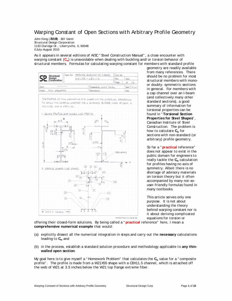
Warping Constant of Open Sections with Arbitrary Profile Geometry John Fong (馮永康) . Bill Vanni Structural Design Corporation 1133 Claridge Dr., Libertyville, IL 60048 ©July-August 2010

As it appears in several editions of AISC “Steel Construction Manual”, a close encounter with warping constant (Cw) is unavoidable when dealing with buckling and/or torsion behavior of structural members. Formulas for calculating warping constant for members with standard profile

geometry are readily available from many references. There should be no problem for most structural members with mono- or doubly- symmetric sections in general. For members with a cap channel over an I-beam (and collectively many other standard sections), a good summary of information for torsional properties can be found in “Torsional Section Properties for Steel Shapes”, Canadian Institute of Steel Construction. The problem is how to calculate Cw for sections with non-standard (or arbitrary) profile geometry.

So far a “practical reference” does not appear to exist in the public domain for engineers to really tackle the Cw calculation for profiles having no axis of symmetry. Albeit there is no shortage of advisory materials on torsion theory but it often accompanied by many not-so-user-friendly formulas found in many textbooks.

This article serves only one purpose. It is not about understanding the theory behind warping constant nor is it about deriving complicated equations for torsion or

offering their closed-form solutions. By being called a “practical reference” here, I mean a comprehensive numerical example that would:

(a) explicitly dissect all the numerical integration in steps and carry out the necessary calculations leading to Cw and

(b) in the process, establish a standard solution procedure and methodology applicable to any thin-walled open section.

My goal here is to give myself a “Homework Problem” that calculates the Cw value for a “composite profile”. The profile is made from a W21X55 shape with a C8X11.5 channel, which is attached off the web of W21 at 3.5 inches below the W21 top flange extreme fiber.


For easy reference, all the calculation (Calc) pages prepared manually for this homework problem are scanned in as part of this article. It takes seventeen (17) steps to complete the task, hopefully without hiding much of the technical fine points. “Seventeen” is not a sacred number. This task can take a greater number of or fewer steps to suit our needs. It all depends on (a) how familiar we are with the subject, (b) how we organize the presentation, and (c) how much detail we want to expose, add, hide or omit.

Let us get started now: Our example profile is taken after a real-life girder from a mill building. It looks innocent and does not appear much different from some of the classic profiles that we are all familiar with: “a cap channel over an I-beam”, which exists in so many industrial facilities except that our channel is a few inches off from both (the major and minor) axes.

I recommend that you now take a break from reading any further and skim through these Calc pages briefly to get some ideas, especially if you are just curious about why it takes so many steps to figure out a “simple” Cw constant for members with such “simple” profile geometry.

As I go through with steps (and pages) of the Calc in the ensuing paragraphs, some subject(s) that appear trivial or self-explanatory will be bypassed for obvious reasons. Meanwhile I will highlight a few tips or traps here and there wherever appropriate. Anyhow, if you are new to this attempt, please pay closer attention to the “Process” in problem solving techniques rather than in numerical details.

Middle Line Profile Cw Model

Our “Cw model” found on Calc page 1 resembles a typical plane frame model employed in regular structural analysis. The so-called “middle line”

suggests that all the framework linkages in the model would always traverse along the line of mid-thickness of each and every profile component regardless to how thick each may be. Middle line model is an idealized skeleton profile. It is nothing but a graphical description of the general element “geometry” and the element “connectivity”.

For profiles with plain elements, their design is mostly controlled by “strength requirement”. Many rolled shapes having simple flanges and/or webs fit in this category. Constructing a middle line model for these profiles is straightforward as if drawing elements by connecting the dots. Take a plain I-beam for instance, we would “idealize” it with nominal six (6) nodes to depict (or digitize) all the participating components, which include two (2) flange elements and one (1) web element.


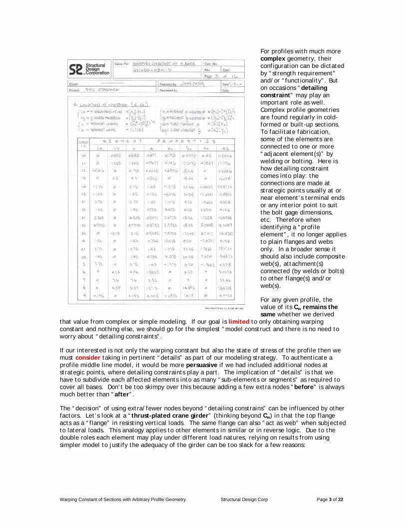
For profiles with much more complex geometry, their configuration can be dictated by “strength requirement” and/or “functionality”. But on occasions “detailing constraint” may play an important role as well. Complex profile geometries are found regularly in cold-formed or built-up sections. To facilitate fabrication, some of the elements are connected to one or more “adjacent element(s)” by welding or bolting. Here is how detailing constraint comes into play: the connections are made at strategic points usually at or near element’s terminal ends or any interior point to suit the bolt gage dimensions, etc. Therefore when identifying a “profile element”, it no longer applies to plain flanges and webs only. In a broader sense it should also include composite web(s), attachment(s) connected (by welds or bolts) to other flange(s) and/or web(s).

For any given profile, the value of its Cw remains the same whether we derived

that value from complex or simple modeling. If our goal is limited to only obtaining warping constant and nothing else, we should go for the simplest “model construct and there is no need to worry about “detailing constraints”.

If our interested is not only the warping constant but also the state of stress of the profile then we must consider taking in pertinent “details” as part of our modeling strategy. To authenticate a profile middle line model, it would be more persuasive if we had included additional nodes at strategic points, where detailing constraints play a part. The implication of “details” is that we have to subdivide each affected elements into as many “sub-elements or segments” as required to cover all bases. Don’t be too skimpy over this because adding a few extra nodes “before” is always much better than “after”.

The “decision” of using extra/fewer nodes beyond “detailing constrains” can be influenced by other factors. Let’s look at a “thrust-plated crane girder” (thinking beyond Cw) in that the top flange acts as a “flange” in resisting vertical loads. The same flange can also ”act as web” when subjected to lateral loads. This analogy applies to other elements in similar or in reverse logic. Due to the double roles each element may play under different load natures, relying on results from using simpler model to justify the adequacy of the girder can be too slack for a few reasons:


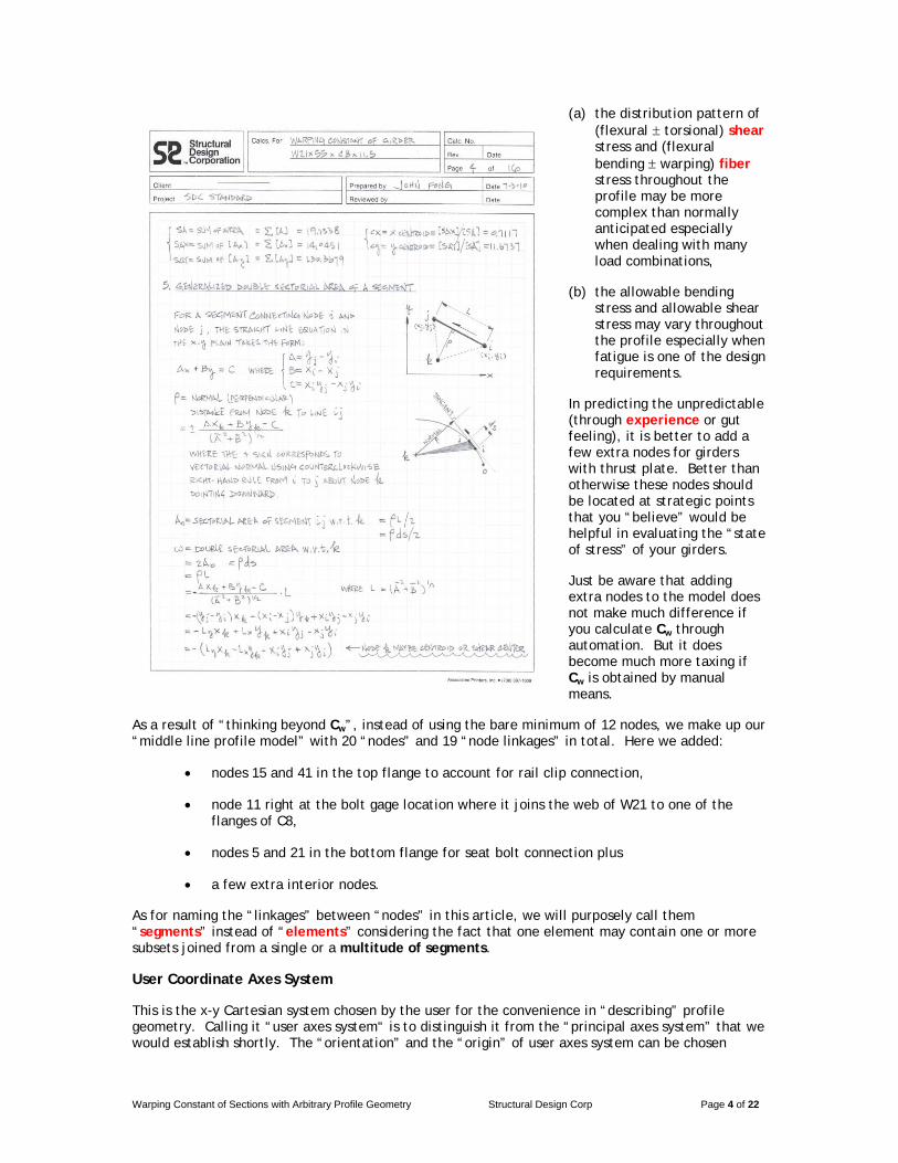
(a) the distribution pattern of (flexural torsional) shear stress and (flexural bending warping) fiber stress throughout the profile may be more complex than normally anticipated especially when dealing with many load combinations,

(b) the allowable bending stress and allowable shear stress may vary throughout the profile especially when fatigue is one of the design requirements.

In predicting the unpredictable (through experience or gut feeling), it is better to add a few extra nodes for girders with thrust plate. Better than otherwise these nodes should be located at strategic points that you “believe” would be helpful in evaluating the “state of stress” of your girders.

Just be aware that adding extra nodes to the model does not make much difference if you calculate Cw through automation. But it does become much more taxing if Cw is obtained by manual means.

As a result of “thinking beyond Cw”, instead of using the bare minimum of 12 nodes, we make up our “middle line profile model” with 20 “nodes” and 19 “node linkages” in total. Here we added:

nodes 15 and 41 in the top flange to account for rail clip connection,

node 11 right at the bolt gage location where it joins the web of W21 to one of the flanges of C8,

nodes 5 and 21 in the bottom flange for seat bolt connection plus

a few extra interior nodes.

As for naming the “linkages” between “nodes” in this article, we will purposely call them “segments” instead of “elements” considering the fact that one element may contain one or more subsets joined from a single or a multitude of segments.

User Coordinate Axes System

This is the x-y Cartesian system chosen by the user for the convenience in “describing” profile geometry. Calling it “user axes system“ is to distinguish it from the “principal axes system” that we would establish shortly. The “orientation” and the “origin” of user axes system can be chosen


arbitrarily. The liberty in choices does not apply to principal axes system for it is unique to a given profile.

Before locating the “origin” of the user system, let us define the “y-axis” to be collinear with the centerline of the web of W21. As for the “x-axis”, I prefer to have it lined up with the bottom extreme fiber of the bottom flange. You can verify on Calc page 1 the location of the “user system origin” based on this scheme. You may have it any other ways per your convenience but here are some of the advantages of my preference:

(a) the y-coordinate for all the nodes would always be positive that we should appreciate later for not having to mess with so many numbers with negative sign many times over;

(b) it would facilitate the re-assignment of nodal y-coordinates due to any revision in segment attributes especially changing in bottom flange thickness.

Data Input

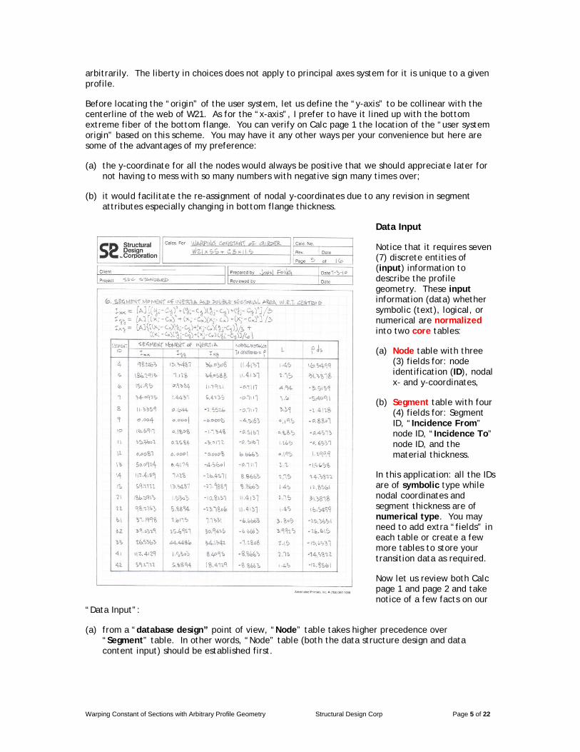
Notice that it requires seven (7) discrete entities of (input) information to describe the profile geometry. These input information (data) whether symbolic (text), logical, or numerical are normalized into two core tables:

(a) Node table with three (3) fields for: node identification (ID), nodal x- and y-coordinates,

(b) Segment table with four (4) fields for: Segment ID, “Incidence From” node ID, “Incidence To” node ID, and the material thickness.

In this application: all the IDs are of symbolic type while nodal coordinates and segment thickness are of numerical type. You may need to add extra “fields” in each table or create a few more tables to store your transition data as required.

Now let us review both Calc page 1 and page 2 and take notice of a few facts on our

“Data Input”:

(a) from a “database design” point of view, “Node” table takes higher precedence over “Segment” table. In other words, “Node” table (both the data structure design and data content input) should be established first.


(b) the numbering system for both “Node” and “Segment” IDs is entirely arbitrary. We have choices of using “numerals” or “text characters”. Professionally we should use “text characters” for purpose of “identification” (not for “calculation”).

(c) as for the “segment end incidences”, there is no set pattern on which end should be the “From” node or which should be the “To” node. One of the rules we must adhere to is that any (input) node ID used for specifying segment connectivity purpose should already be defined in the “Node table” (thereby maintaining the Data Referential Integrity);

(d) typical segment should always follow a rule to have uniform thickness between its “From” node and “To” node. In dealing with change in thickness within a segment, we must add extra node(s) in between making all segments comply with the thickness rule.

(e) material thickness for segments joined by weld or bolt should be additive from all the participating segments. Using the “resulting thickness sum” is to simulate that these segments are “fused” into one idealized (combined) segment.

For instance: web thickness of W21 = 0.375 and flange thickness of C8 = 0.39. For segments 10 and 11 being joined by bolt at node 11, we would use combined thickness = 0.765 replicating that the W21 web and C8 flange would react in unison under loads;

(f) for any “fused segment” transitioning contiguously to the immediate adjacent “clean-and-free-from-joining element”, the thickness should be considered “insignificant”. Such “segment” does not really exist. Its presence is only for model “linkage purpose” therefore we may assign a value that is relatively trivial comparing to the thickness of all other “significant” segments in the profile. As in our example for segments 9 and 12: we would assign a fictitious thickness = 0.001.

Data Presentation

The “usefulness” of calculation is measured primarily by the “numerical accuracy”. Numerical mistakes found in engineering calculation are very much avoidable but inevitable because not every Preparer is perfect. This is why some calculations must be reviewed for quality assurance purpose.


The bottom line is to catch the mistake and fix it in time. The amount of time it takes for a Reviewer to “review” depends somewhat on how appealing the information was arranged. If the “presentation” were clear to the Preparer, then it would take much less effort for the Reviewer to “identify” and “rectify” the mistake(s) should there be any.

Engineering calculation is a presentation of processes. Each process follows a preset routine. When we design a beam, the process may involve writing down dimensions, setting up applied loads, calculating internal forces and moments, applied stresses and allowable stresses, etc. Each beam is treated as a separate entity. The documentation for designing a beam follows a top-down line-by-line style. In calculating warping constant, the process also follows a top-down style but with a twist. It involves many cycles of marching forward for new data then referencing backward for existing data much as in a zigzag. In addition, to carry out each step the entire data set gets involved. In other words, if we execute nodal (segment) data, information related all 20 nodes (19

segments) would get the same mass-production treatment.

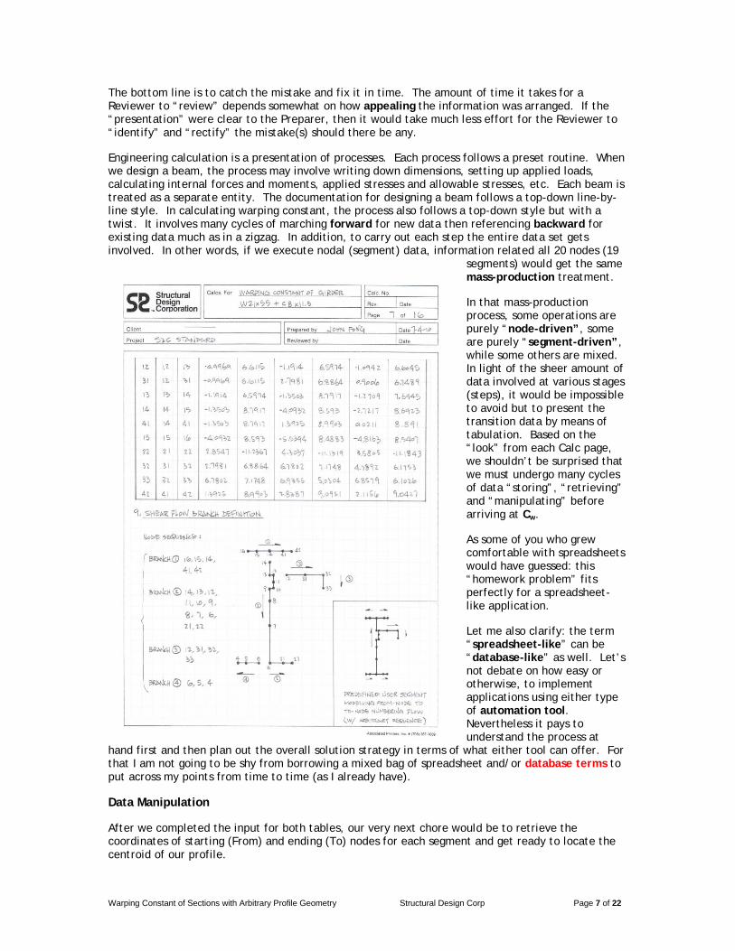
In that mass-production process, some operations are purely “node-driven”, some are purely “segment-driven”, while some others are mixed. In light of the sheer amount of data involved at various stages (steps), it would be impossible to avoid but to present the transition data by means of tabulation. Based on the “look” from each Calc page, we shouldn’t be surprised that we must undergo many cycles of data “storing”, “retrieving” and “manipulating” before arriving at Cw.

As some of you who grew comfortable with spreadsheets would have guessed: this “homework problem” fits perfectly for a spreadsheet-like application.

Let me also clarify: the term “spreadsheet-like” can be “database-like” as well. Let’s not debate on how easy or otherwise, to implement applications using either type of automation tool. Nevertheless it pays to understand the process at

hand first and then plan out the overall solution strategy in terms of what either tool can offer. For that I am not going to be shy from borrowing a mixed bag of spreadsheet and/or database terms to put across my points from time to time (as I already have).

Data Manipulation

After we completed the input for both tables, our very next chore would be to retrieve the coordinates of starting (From) and ending (To) nodes for each segment and get ready to locate the centroid of our profile.


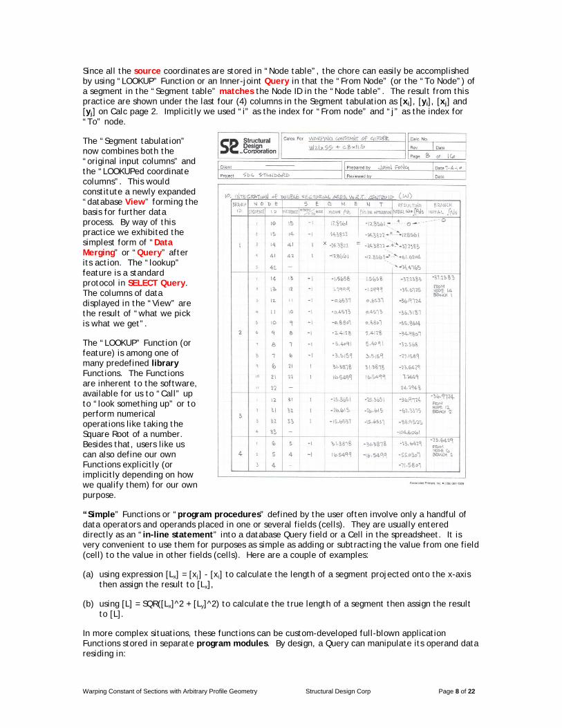
Since all the source coordinates are stored in “Node table”, the chore can easily be accomplished by using “LOOKUP” Function or an Inner-joint Query in that the “From Node” (or the “To Node”) of a segment in the “Segment table” matches the Node ID in the “Node table”. The result from this practice are shown under the last four (4) columns in the Segment tabulation as [xi], [yi], [xj] and [yj] on Calc page 2. Implicitly we used “i” as the index for “From node” and “j” as the index for “To” node.

The “Segment tabulation” now combines both the “original input columns” and the “LOOKUPed coordinate columns”. This would constitute a newly expanded “database View” forming the basis for further data process. By way of this practice we exhibited the simplest form of “Data Merging” or “Query” after its action. The “lookup” feature is a standard protocol in SELECT Query. The columns of data displayed in the “View” are the result of “what we pick is what we get”.

The “LOOKUP” Function (or feature) is among one of many predefined library Functions. The Functions are inherent to the software, available for us to “Call” up to “look something up” or to perform numerical operations like taking the Square Root of a number. Besides that, users like us can also define our own Functions explicitly (or implicitly depending on how we qualify them) for our own purpose.

“Simple” Functions or “program procedures” defined by the user often involve only a handful of data operators and operands placed in one or several fields (cells). They are usually entered directly as an “in-line statement” into a database Query field or a Cell in the spreadsheet. It is very convenient to use them for purposes as simple as adding or subtracting the value from one field (cell) to the value in other fields (cells). Here are a couple of examples:

(a) using expression [Lx] = [xj] - [xi] to calculate the length of a segment projected onto the x-axis then assign the result to [Lx],

(b) using [L] = SQR([Lx]^2 + [Ly]^2) to calculate the true length of a segment then assign the result to [L].

In more complex situations, these functions can be custom-developed full-blown application Functions stored in separate program modules. By design, a Query can manipulate its operand data residing in:


(a) a single table or several discrete tables, and/or involving

(b) other sibling Queries (participating as sub-queries) through data links (or none at all)

to create a new database “View”.

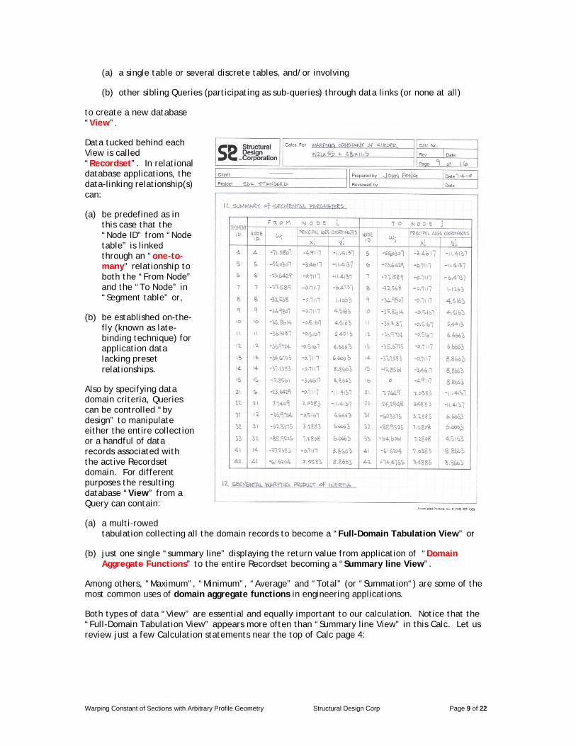
Data tucked behind each View is called “Recordset”. In relational database applications, the data-linking relationship(s) can:

(a) be predefined as in this case that the “Node ID” from “Node table” is linked through an “one-to-many” relationship to both the “From Node” and the “To Node” in “Segment table” or,

(b) be established on-the-fly (known as late-binding technique) for application data lacking preset relationships.

Also by specifying data domain criteria, Queries can be controlled “by design” to manipulate either the entire collection or a handful of data records associated with the active Recordset domain. For different purposes the resulting database “View” from a Query can contain:

(a) a multi-rowed tabulation collecting all the domain records to become a “Full-Domain Tabulation View” or

(b) just one single “summary line” displaying the return value from application of “Domain Aggregate Functions” to the entire Recordset becoming a “Summary line View”.

Among others, “Maximum”, “Minimum”, “Average” and “Total” (or “Summation“) are some of the most common uses of domain aggregate functions in engineering applications.

Both types of data “View” are essential and equally important to our calculation. Notice that the “Full-Domain Tabulation View” appears more often than “Summary line View” in this Calc. Let us review just a few Calculation statements near the top of Calc page 4:


(a) terms [SA], [SAX] and [SAY] are the results from applying “Summation” (Domain Aggregate Function) to terms [A], [SA] and [SY], respectively from Segment Properties’ Recordset already tabulated on Calc page 3.

(b) The “Summary line View” had been subtly hidden behind the scene in the Calc. Instead of tabulating them I had expressed the results as if I manually calculated the centroid coordinates [cx] and [cy].

Principal Axes

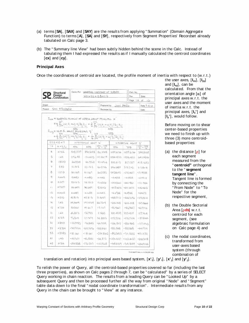
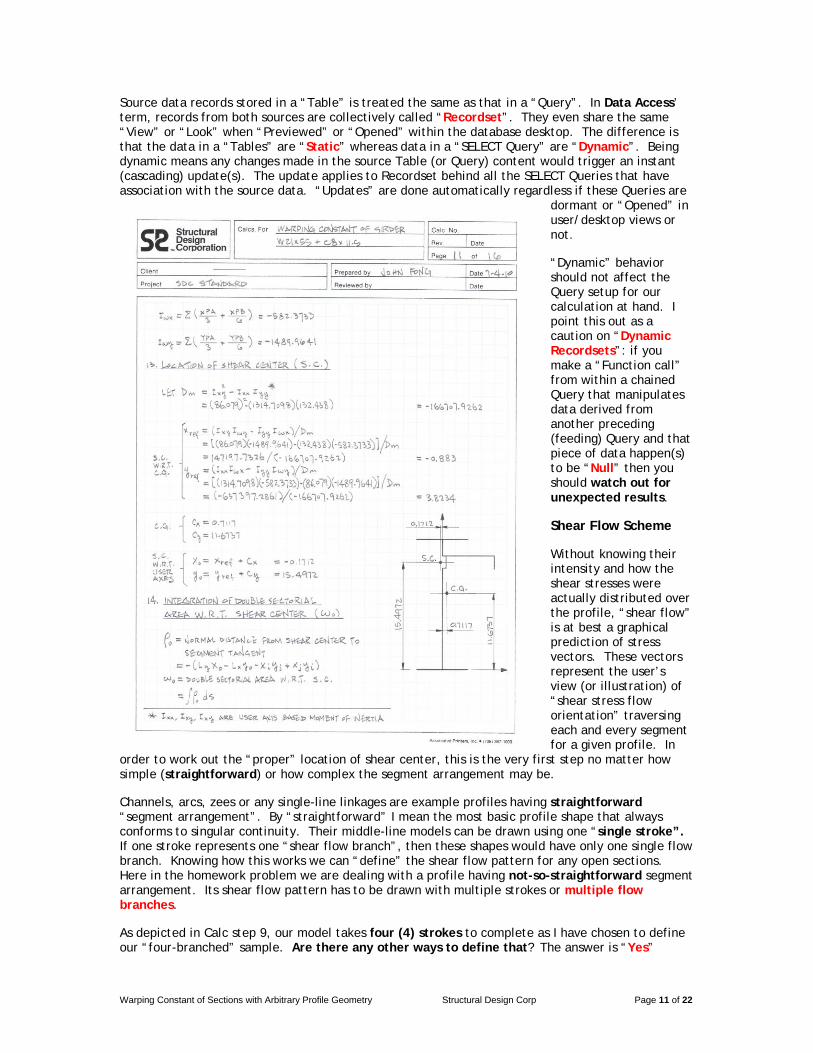
Once the coordinates of centroid are located, the profile moment of inertia with respect to (w.r.t.) the user axes, [Ixx], [Iyy] and [Ixy], can be calculated. From that the orientation angle [] of principal axes w.r.t. the user axes and the moment of inertia w.r.t. the principal axes, [Ix’] and [Iy’], would follow.

Before moving on to shear center-based properties we need to finish up with three (3) more centroid-based properties:

(a) the distance [] for each segment measured from the “centroid” orthogonal to the “segment tangent line”. Tangent line is formed by connecting the “From Node” to “To Node” for the respective segment,

(b) the Double Sectorial Area [ds] w.r.t. centroid for each segment, (see algebraic formulation on Calc page 4) and

(c) the nodal coordinates, transformed from user-axes based system (through combination of

translation and rotation) into principal axes based system, [x’i], [y’i], [x’j] and [y’j].

To relish the power of Query, all the centroid-based properties covered so far (including the last three properties), as shown on Calc pages 2 through 7, can be “calculated” by a series of SELECT Query working in chain reaction. The results from a leading Query can be “Looked Up” by a subsequent Query and then be processed further all the way from original “Node” and “Segment” table data down to the final “nodal coordinate transformation”. Intermediate results from any Query in the chain can be brought to “View” at any instance.


Source data records stored in a “Table” is treated the same as that in a “Query”. In Data Access’ term, records from both sources are collectively called “Recordset”. They even share the same “View” or “Look” when “Previewed” or “Opened” within the database desktop. The difference is that the data in a “Tables” are “Static” whereas data in a “SELECT Query” are “Dynamic”. Being dynamic means any changes made in the source Table (or Query) content would trigger an instant (cascading) update(s). The update applies to Recordset behind all the SELECT Queries that have association with the source data. “Updates” are done automatically regardless if these Queries are

dormant or “Opened” in user/desktop views or not.

“Dynamic” behavior should not affect the Query setup for our calculation at hand. I point this out as a caution on “Dynamic Recordsets”: if you make a “Function call” from within a chained Query that manipulates data derived from another preceding (feeding) Query and that piece of data happen(s) to be “Null” then you should watch out for unexpected results.

Shear Flow Scheme

Without knowing their intensity and how the shear stresses were actually distributed over the profile, “shear flow” is at best a graphical prediction of stress vectors. These vectors represent the user’s view (or illustration) of “shear stress flow orientation” traversing each and every segment for a given profile. In

order to work out the “proper” location of shear center, this is the very first step no matter how simple (straightforward) or how complex the segment arrangement may be.

Channels, arcs, zees or any single-line linkages are example profiles having straightforward “segment arrangement”. By “straightforward” I mean the most basic profile shape that always conforms to singular continuity. Their middle-line models can be drawn using one “single stroke”. If one stroke represents one “shear flow branch”, then these shapes would have only one single flow branch. Knowing how this works we can “define” the shear flow pattern for any open sections. Here in the homework problem we are dealing with a profile having not-so-straightforward segment arrangement. Its shear flow pattern has to be drawn with multiple strokes or multiple flow branches.

As depicted in Calc step 9, our model takes four (4) strokes to complete as I have chosen to define our “four-branched” sample. Are there any other ways to define that? The answer is “Yes”


provided that we follow a certain “scheme”. Let us draw the strokes in “unidirectional manner” using my Scheme for this example:

(a) starting arbitrarily the 1st flow branch from any terminal node, say node [16];

(b) moving along segments at will through as many nodes [15, 14, 41,...] as we encounter in between;

(c) finishing the 1st flow branch upon reaching another terminal node [42];

(d) diverging the 2nd branch off any interfacing node, say node [14] from the 1st branch then completing the 2nd branch as in steps (b) and (c) [14, 13, 12,...21, 22];

(e) diverging subsequent branches off from a node on any established branches the same way until depleting all segments without duplicating usage of any one of them.

Imagine if it were a “tree structure”, we may visualize the 1st branch as “trunk” and all the other offshoot branches as “twigs”. Here is another example following the same “scheme” but taking different routes that we end up with:

(a) branch 1 as: from node 16, 15, 14, 13, 12, 31, 32 to 33;

(b) branch 2 as: from node 12, 11, 10, 9, 8, 7, 6, 5 then 4;

(c) branch 3 as: from node 14, 41 to 42; and

(d) branch 4 as: from 6, 21 to 22, or any other arrangement(s).

Notice that the flow “direction” along these branches defined in both examples does not conform to any explicit rule in sign conventions. In other words, both examples employed no assumptions on the generic positive (or negative) flow senses. Neither has it any bearing on how the segment nodal incidences were assigned in the original Segment input (see inset at lower right-hand corner on Calc page 7).

Therefore it really doesn’t matter how “wrong” our prediction on the stress flow “senses” that may be. Consequently all the “wrongs”, if ever true, would be “corrected automatically” after all the numerical integrations are completed. This “auto-correction” would work for any profile geometry so long as their branch assignments and the associated “node sequences” were set up consistently using this “scheme”.

Once they are finalized, it is important to store the shear flow branch data. Because we have to refer to them for at least three (3) times from here on, it’s preferable to save them in a table rather than plain program variables (arrays). This important table we may name it “ShearFlowID”, “ShearFlowBranches”, or simply “Branches”.

The “Branches” table should have at least four (4) fields to store:

(a) Shear Flow Branch ID,

(b) Nodal Sequence (Serial) ID,

(c) Node ID and

(d) Incidence Segment ID.

Much have I tried, there seems to be no “practical way” to derive the “shear flow definition data” using database “Queries” alone. In two ways we can prepare the records for “Branches” table by:

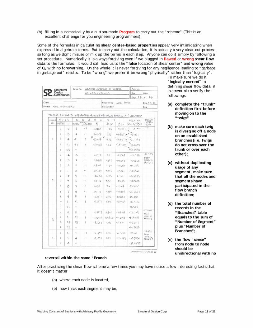
(a) filling in manually after defining shear flow branches on a sketch similar to that as shown in step 9 on Calc page 8, or


(b) filling in automatically by a custom-made Program to carry out the “scheme” (This is an excellent challenge for you engineering programmers).

Some of the formulas in calculating shear center-based properties appear very intimidating when expressed in algebraic terms. But to carry out the calculation, it is actually a very clear-cut process so long as we don’t misuse or mix up the terms in each step. Anyone can do it simply by following a set procedure. Numerically it is always forgiving even if we plugged in flawed or wrong shear flow data to the formulas. It would still lead us to the “false location of shear center” and wrong value of Cw with no forewarning. On the whole it is never forgiving for any negligence leading to “garbage in garbage out” results. To be “wrong” we prefer it be wrong “physically” rather than “logically”.

To make sure we do it “logically correct” in defining shear flow data, it is essential to verify the followings:

(a) complete the “trunk” definition first before moving on to the “twigs”

(b) make sure each twig is diverging off a node on an established branches (i.e. twigs do not cross over the trunk or over each other);

(c) without duplicating usage of any segment, make sure that all the nodes and segments have participated in the flow branch definition;

(d) the total number of records in the “Branches” table equals to the sum of “Number of Segment” plus “Number of Branches”;

(e) the flow “sense” from node to node should be unidirectional with no

reversal within the same “Branch.

After practicing the shear flow scheme a few times you may have notice a few interesting facts that it doesn’t matter

(a) where each node is located,

(b) how thick each segment may be,


(c) how many strokes it took to draw up the profile and

(d) how we sequence the nodes.

I point this out to prove a point that shear flow scheme is a “pure logic process”. Our “scheme” utilizes only three (3) items: Segment ID, Segment From-node and To-node IDs from “Segment” table without incurring any reference to “Node table” at all. The logic sounds simple but could be a real challenge to automate the shear flow assignment process together and the ensuing procedures for numerical integrations toward Cw.

Double Sectorial Area w.r.t. Centroid ()

“Summation” is the simplest form of numerical integration. Recall that we first applied “Summation” method to locate the profile centroid and then obtain the user-axes based moment of inertia. This method unfortunately does not work for integration of Double Sectoria Area (DSA) and other “shear flow-related integrations”. Instead we must proceed in a step-by step (node-by-node)

manner. Here is how it works in a nutshell, the “succeeding value” of integration at any intermediate step is dependent on:

(a) its own attributes and

(b) the “preceding value” determined from a previous step.

This suggests that we must progress the nodal data integration in an ascending (or descending) order according to the shear flow logic.

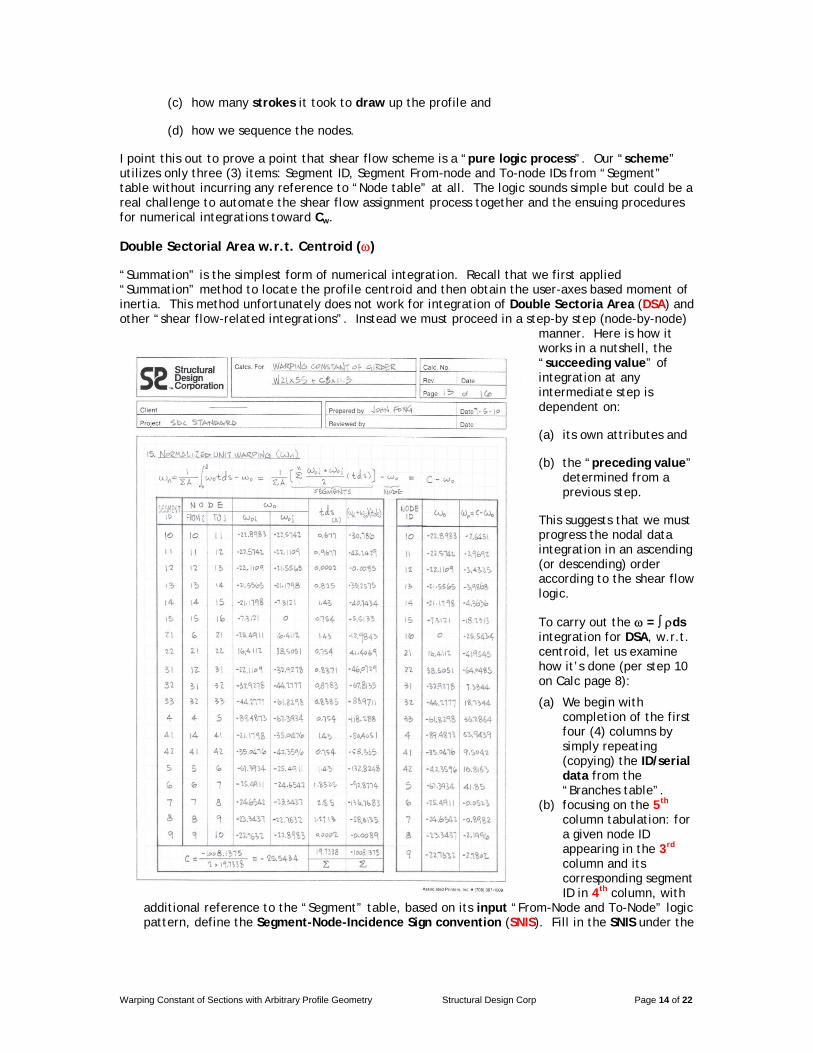
To carry out the = ds integration for DSA, w.r.t. centroid, let us examine how it’s done (per step 10 on Calc page 8):

(a) We begin with completion of the first four (4) columns by simply repeating (copying) the ID/serial data from the “Branches table”.

(b) focusing on the 5th column tabulation: for a given node ID appearing in the 3rd column and its corresponding segment ID in 4th column, with

additional reference to the “Segment” table, based on its input “From-Node and To-Node” logic pattern, define the Segment-Node-Incidence Sign convention (SNIS). Fill in the SNIS under the


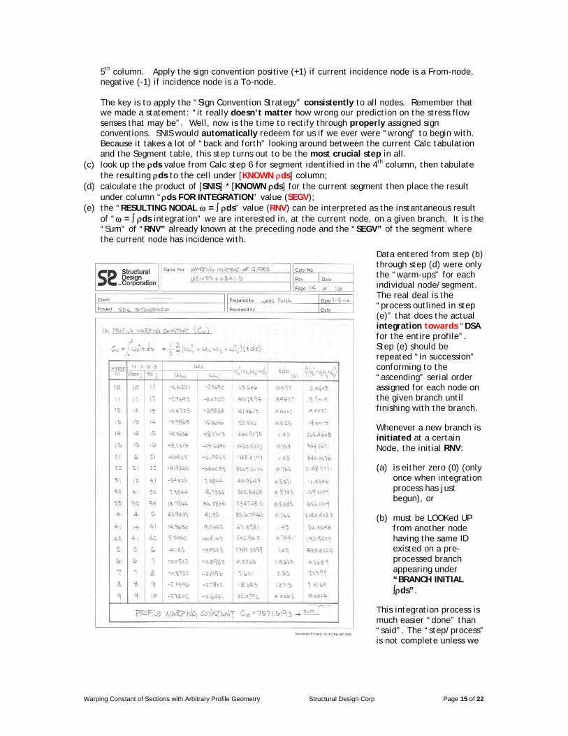
5th column. Apply the sign convention positive (+1) if current incidence node is a From-node, negative (-1) if incidence node is a To-node.

The key is to apply the “Sign Convention Strategy” consistently to all nodes. Remember that we made a statement: “it really doesn’t matter how wrong our prediction on the stress flow senses that may be”. Well, now is the time to rectify through properly assigned sign conventions. SNIS would automatically redeem for us if we ever were “wrong” to begin with. Because it takes a lot of “back and forth” looking around between the current Calc tabulation and the Segment table, this step turns out to be the most crucial step in all.

(c) look up the ds value from Calc step 6 for segment identified in the 4th column, then tabulate the resulting ds to the cell under [KNOWN ds] column;

(d) calculate the product of [SNIS] * [KNOWN ds] for the current segment then place the result under column “ds FOR INTEGRATION” value (SEGV);

(e) the “RESULTING NODAL = ds” value (RNV) can be interpreted as the instantaneous result of “ = ds integration” we are interested in, at the current node, on a given branch. It is the “Sum” of “RNV” already known at the preceding node and the “SEGV” of the segment where the current node has incidence with.

Data entered from step (b) through step (d) were only the “warm-ups” for each individual node/segment. The real deal is the “process outlined in step (e)” that does the actual integration towards “DSA for the entire profile”. Step (e) should be repeated “in succession” conforming to the “ascending” serial order assigned for each node on the given branch until finishing with the branch.

Whenever a new branch is initiated at a certain Node, the initial RNV:

(a) is either zero (0) (only once when integration process has just begun), or

(b) must be LOOKed UP from another node having the same ID existed on a pre-processed branch appearing under “BRANCH INITIAL ds”.

This integration process is much easier “done” than “said”. The “step/process” is not complete unless we


carried out fully from branch 1, node serial 1 all the way through the last node on the last branch. A sample worked-out on the “Node-driven” data flow for branch #1 can be traced by following the dotted arrow as shown on Calc page 8.

Warping Moment of Inertia

“Warping Moment of Inertia” about Principal x’ and y’ Axes (WMOIPA) are designated as Ix and Iy, respectively. They carry a dimension unit of (Length)5 versus the (Length)4 for Flexural Moment of Inertia.

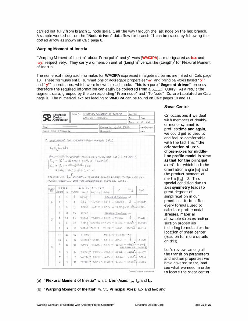
The numerical integration formulas for WMOIPA expressed in algebraic terms are listed on Calc page 10. These formulas entail summations of aggregate properties “” and principal-axes based “x’” and “y’” coordinates, which were known at each node. This is a pure “Segment-driven” process therefore the required information can easily be collected from a SELECT Query. As a result the segment data, grouped by the corresponding “From node” and “To Node” IDs, are tabulated on Calc page 9. The numerical excises leading to WMOIPA can be found on Calc pages 10 and 11.

Shear Center

On occasions if we deal with members of doubly- or mono- symmetric profiles time and again, we could get so used to and feel so comfortable with the fact that “the orientation of user-chosen-axes for middle-line profile model is same as that for the principal axes”, for which both the orientation angle [] and the product moment of inertia [Ixy]= 0. This special condition due to axis symmetry leads to great degrees of simplification in our practices. It simplifies every formula used to calculate profile nodal stresses, material allowable stresses and/or section properties including formulas for the location of shear center (read on for more details on this).

Let’s review, among all the transition parameters and section properties we have covered so far, and see what we need in order to locate the shear center:

(a) “Flexural Moment of Inertia” w.r.t. User-Axes; Ixx, Iyy and Ixy

(b) “Warping Moment of Inertial” w.r.t. Principal Axes; Ix and Ix and


(c) coordinates of profile centroid; cx and cy.

Let’s also define a few shear center-related unknowns:

(a) Xref and Yref to be the relative displacements (translation distances) from the profile centroid to the shear center and

(b) xo and yo to be the shear center coordinates based on user-axes system.

Fitting different categories of profile geometry, there are three (3) cases of shear center formulas for Xref and Yref we need to get familiar with.

Case 1: the simplest case applicable to the most obvious member category with doubly- symmetric profiles: the shear center always coincides with the centroid rendering both Xref and Yref = 0, and therefore xo = cx and yo = cy.

Case 2: the most generic case applicable to all other profile geometries (with or without any axis symmetry), we may find them from many textbooks the expressions for calculating the coordinates of shear center as:

Xref = (Ixy * Ix – Iyy * Iy) / (Ixy2 – Ixx * Iyy) (Eq. 1)

Yref = (Ixx * Ix – Ixy * Iy) / (Ixy2 – Ixx * Iyy) (Eq. 2)

If we apply them to mono- symmetric sections by setting Ixy = 0, then they can be simplified into Case 3:

Xref = Iy / Ixx (Eq. 3)

Yref = - Ix / Iyy (Eq. 4)

It happens that in some textbooks where you may find Eq. 3 and Eq. 4 given as the formulas for shear center calculation with no mentioning that they are only applicable to mono-symmetric profiles.

If we were “new to the task” of locating shear center without further checking and blindly following (applying) Eq. 3 and Eq. 4 to a section having no axes of symmetry, we would still be able to obtain Xref and Yref but in fact these formulas (results) were wrong for the occasion. We must be careful about the trap I mentioned in the first paragraph on this matter. If you plan to automate your calculation I recommend that you always use Eq. 1 and Eq. 2.

Finally by parallel shifting w.r.t. centroid, the coordinates of shear center per user-axes are:

xo = Xref + cx

yo = Yref + cy

Double Sectorial Area w.r.t. Shear Center (o)

Our next assignment per Calc step 14 (Calc page 11) is to perform integration for o , which is the “DSA w.r.t. Shear Center”. In its integration formula o = ods, the term o looks familiar but is actually a new term.

Let’s go back to the formula for DSA w.r.t. centroid = ds and recall that is the normal distance from centroid to the segment tangent. Here the only difference is that o is used in place of , where o is the normal distance from shear center to the segment tangent. Obviously the formulas for figuring out the geometry of and o resemble each other if you check the Calc.


This is the second process involving shear flow-related data. Starting with the same shear flow branch definitions, the numerical procedure for o = ods is “almost identical” to that as described in the calculation for = ds. A worked-out “Node-driven” data flow for shear flow branch #1 can be traced by following the dotted arrows as shown on Calc page 12. I would leave it up to you to “see” any difference between and o.

Normalized Unit Warping (n) and Warping Constant (Cw)

“Normalized Unit Warping” is designated as n. The formula for n expressed in algebraic terms is shown on Calc page 13. It entails summations of nodal property “o“ and the cross sectional area of segment “tds”. This would require a two-step procedure to arrive at o because one of the two (2) terms is a profile “constant” and the other is a nodal “variable”. The first step involves a “Segment-driven” process that integrates (o tds) of each segment over the entire profile into a constant “C”. The second step is simply a “Node-driven” process that subtracts “o” from “C” to arrive at n at each node as shown on Calc page 13. The procedure for calculating warping constant becomes fairly simple once the corresponding values of “tds” and “n“ have been:

(a) “collected” from all nodes and

(b) “grouped” by incidence nodes with respective to each segment.

Using a SELECT Query for the “grouping” followed by a “Summation”, we finally complete the calculation of Cw constant for our example by way of “classic method” (see resulting tabulations per Step 16 on Calc page 14). I call it a “classic method” because the undertaking was achieved by performing numerical integration for “formulas” derived from “classic torsion theory”. Here are some of the disadvantages from using “classic solution method” as demonstrated:

(a) tedious and time consuming

(b) confusing every so often

(c) full of numerical traps throughout the process.

Besides classic solution method there are other methods we can use to avoid all that. Some of these are so called the “direct method” or “displacement method”. Without knowing anything about principal axes, the “direct” formulation would lead to solution of “xo”, “yo” and all the nodal n values in one shot. Better yet we don’t even need “shear flow definition”. This sounds fantastic and is a good trade off for not having to mess with numerical integration. However the most cumbersome chores in implementing these methods are: (1) setting up the property-geometry matrices and (2) solving for the ensuing simultaneous equations. Applying direct method to solve for n and shear center coordinates for our example profile of 20 nodes would require inversion of a 22X22 matrix.

Warping Static Moment (Sw)

“Warping Static Moment” (WSM) is another warping-related property designated as Sw. Values of WSM must be known at each node before the “state of warping shear stress” of a profile can be evaluated. Even if your interest is in Cw or n only and you have no desire to go any further, I still recommend that you follow through with this important subject if your member has arbitrary profile geometry.

In the simplest case for sections having doubly- or mono- symmetric profile, we can easily verify if the nodal n values are distributed consistently and evenly about the matching axis of symmetry to “see” immediately if we “made any mistake”. But for sections with no axis of symmetry, there is no easy way (or no way) to validate the adequacy of warping-related properties (both n and Cw). Warping constant Cw comes form a chain reaction involving a full course of profile properties, to name a few:


centroid, neutral axes, user-axes moment of inertia, principal-axes moment of inertia, shear flow data, shear center, , o , o and n, etc.

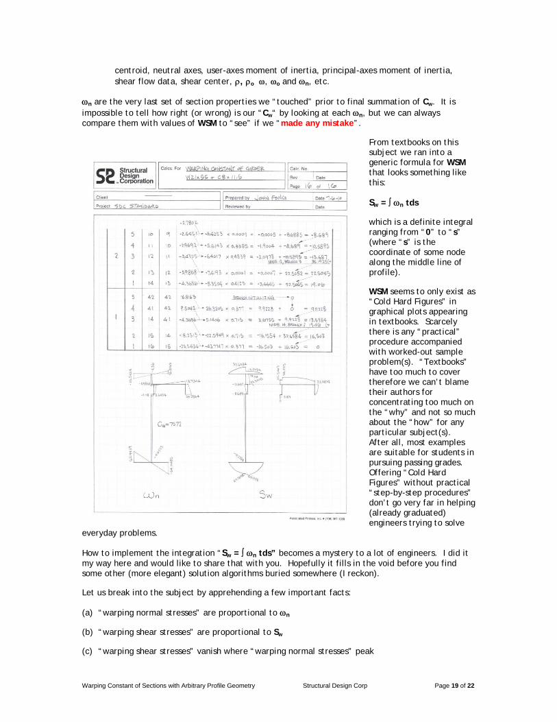
n are the very last set of section properties we “touched” prior to final summation of Cw. It is impossible to tell how right (or wrong) is our “Cw“ by looking at each n, but we can always compare them with values of WSM to “see” if we “made any mistake”.

From textbooks on this subject we ran into a generic formula for WSM that looks something like this:

Sw = n tds

which is a definite integral ranging from “0” to “s” (where “s” is the coordinate of some node along the middle line of profile).

WSM seems to only exist as “Cold Hard Figures” in graphical plots appearing in textbooks. Scarcely there is any “practical” procedure accompanied with worked-out sample problem(s). “Textbooks” have too much to cover therefore we can’t blame their authors for concentrating too much on the “why” and not so much about the “how” for any particular subject(s). After all, most examples are suitable for students in pursuing passing grades. Offering “Cold Hard Figures” without practical “step-by-step procedures” don’t go very far in helping (already graduated) engineers trying to solve

everyday problems.

How to implement the integration “Sw = n tds” becomes a mystery to a lot of engineers. I did it my way here and would like to share that with you. Hopefully it fills in the void before you find some other (more elegant) solution algorithms buried somewhere (I reckon).

Let us break into the subject by apprehending a few important facts:

(a) “warping normal stresses” are proportional to n

(b) “warping shear stresses” are proportional to Sw

(c) “warping shear stresses” vanish where “warping normal stresses” peak


(d) “warping normal stresses” always peak at terminal ends (nodes)

(e) “warping shear stresses” equal to zero at terminal nodes and peak where “warping normal stresses” vanish

(f) therefore Sw equals to zero at terminal nodes

These can be verified by inspecting the “n“ (already known) and “Sw“ (not yet calculated) values as plotted on Calc page 16. We only need to compare the respective magnitude at terminal nodes 16, 42, 33, 4 and 22 to substantiate if we erred.

I mentioned earlier that the “shear flow information” would be used for at least three (3) times:

(a) first: “ = ds” integral of DSA w.r.t.centroid,

(b) second: similarly the “o = ods” integral of DSA w.r.t. shear center,

(c) and now the third: somewhat differently the “Sw = n tds” integral of WSM.

Words “similarly” and “somewhat differently” refer to “how we sequence” the “shear flow branch information” during integration. The path taken on for DSA integration follows an “ascending flow” while in WSM it follows a “descending flow”. Ascending flow starts from the first branch (#1), first node (#1) and ends at the last branch (#4), last node (#3). Descending flow proceeds along a path in exactly the reverse order.

It’s easy to implement definite integral ranges from “0” to “s” for profiles conform to singular continuity (channels for example). Each of these profiles has only two (2) ends for us to concern about. We simply carry out numerical integration either from one end to the other or vise versa. It is convenient to interpret “0” as one of the terminal ends and “s” being the opposite end (or somewhere in the middle). It doesn’t matter whether we follow ascending or descending order because there is no wrong end.

Problem is how to deal with profiles with multiple terminal ends. If we have not yet gone through Calc pages 15 and 16, we may ask these questions:

(a) how to implement the definite integral ranges from “0” to “s” for the example profile with five (5) terminal ends?

(b) which node to start with?

(c) where does the integration end?

Answers to all these questions are: “Use descending flow”. Here is where it deserves more thorough explanation. “Descending flow” is “somewhat different” from “ascending flow” in the way we handle the “s” portion of the integral. As an excise I would leave it up to you to “see” the difference when this is all said and done.

We recognize that “s” is the intermediate “integration path taken” up to somewhere within the profile boundary. The leading extremity of the “s path” may arrive at anywhere in the vicinity of any given Node. Chances are that it may be (a) right on, (b) nearby or (c) far away from some terminal end in focus. Making things simple we purposely let “s” be “right on” a certain segment’s “From Node” (or “To Node”). From a numerical integration standpoint, it’s easier to deal with start node index “i” and end node index “j” than the adjectives “From” and “To” (although either “i” or “j” can coincide with a “From” or “To” node in physical sense). In terms of integration we would always handle the “segment WSM” sequence from “node i” to “node j”. The path we take must follow the “Descending Flow” along any given branch. The calculated values of WSMs for a typical segment are labeled as Swi for node “i” and Swj at node “j”, respectively.

Let’s go through the Sw algorithm:


(a) process the integration steps (b) through (d) according to the descending flow branch sequence (ex: 4, 3, 2 then 1). In other words, always finish all the “twigs” first and the “trunk” last,

(b) when starting a new branch (from a terminal node), always set Swi = 0,

(c) when starting a typical segment,

a. verify “proper flow vector“ based on whether the “i-j flow” for integration is oriented along the “From-To flow” or along the “To-From flow”,

b. identify which is node “i” and which is node “j”

c. look up the value of n at node “i” as ni

d. set Swi as the summation of all Swi already known at node “i”,

(d) to finish up a typical segment at node “j”,

a. look up the value of n at node “j” as nj

b. look up the value of cross sectional area of segment as “tds”

c. calculate K = (ni + nj) * (tds) / 2

d. set Swj = K + Swi

The worked-out “Node-driven” data flow following Sw algorithm for the entire profile can be traced by the dotted arrows appearing in the tabulation shown on Calc pages 15 and 16. Because Sw must equal to zero at terminal nodes, it is easy to verify if we “made any mistake”. Most importantly we need to make sure Swj = 0 (or approaches zero) at the very last node we processed (i.e. shear flow node serial #1, flow branch #1, or input node 16 on segment 15). If “Sw <> 0” or “Sw does not approach zero”, there is definitely “something wrong” during the process. This has demonstrated that validation of Cw for “profiles with no axis of symmetry” would not be possible without helps from Sw.

It is worthwhile knowing the distribution of WSM throughout the profile is non-linear with intermittent peaks and valleys (PAVS). To pin point where the PAVS are by inspecting Swi and Swj at both ends of segments alone is not enough. Because WSM peaks where “warping normal stress” vanishes, it is easy to locate the PAVS by checking on each segment whether if the product of ni * nj < = 0. If this condition is true then we can locate the point of PAVS by interpolation and calculate the PAVS accordingly. This extra step for PAVS is not necessary unless our interest also include the state of warping shear stress.

Conclusion

The subject in dealing with flexural horizontal shear stress (FHSS) was absent in this article until now for it has nothing to do with warping constant. FHSS is calculated using “VQ/It” formula found in many textbooks on “strength of material”. Property “Q” is called “First moment” or “Moment of area”. When a profile is subjected to both X- and Y- forces, the FHSS should be calculated using both Qx and Qy. To figure out Qx and Qy for sections of arbitrary profile geometry with no axis of symmetry it requires numerical integration w.r.t. the principal axes in steps similar to but slightly different from algorithm used for “Sw”. It should be not so hard to figure out the difference.

In summary, to calculate the warping constant for this example profile with 20 nodes, we probably have to deal with at least 2000 numerical entries plus mathematical operators, parentheses and sign change keys, etc. Through it all you may have sensed that the demand in data management rivals the effort in number crunching. Fine-tuning numerical accuracy against excessive rounding-off and


truncation errors is a tricky chore in itself. An engineering problem suddenly eases itself into a data management problem without realizing it. Therefore the solution process for warping constant is a perfect candidate for automation using database approach.

Documents

Warping Constant of Open Sections with Arbitrary Profile ... Warping Constant (Cw... · Warping Constant of Open Sections with Arbitrary Profile Geometry ... torsional properties