Embed Size (px)
Citation preview

Universita Ca’ Foscari di Venezia
Dipartimento di InformaticaDottorato di Ricerca in Informatica
Ph.D. Thesis: 2009-1
Warehousing and Mining AggregateMeasures Over Trajectories of Moving
Objects
Fernando Jose Braz
Supervisor
Salvatore Orlando
PhD Coordinator
Annalisa Bossi
January, 2009
Author’s e-mail: [email protected]
Author’s address:
Dipartimento di InformaticaUniversita Ca’ Foscari di VeneziaVia Torino, 15530172 Venezia Mestre – Italiatel. +39 041 2348411fax. +39 041 2348419web: http://www.dsi.unive.it

To my wifeTo my daughter
To my familyTo my friends
To those who are not here with me, but from some place are seeing this conquest:my father Aderito and my friends Edson and Irapuan.
God bless you

Abstract
The development of new technologies for mobile devices and low-cost sensors re-sults in the possibility of storing large data volumes about trajectories of movingobjects. In this thesis we propose a multi-dimensional data model to store aggre-gate measures computed over such huge data volumes. This allowed us to define aTrajectory Data Warehouse (TDW ) that is loaded by managing and transforminga data stream of spatio-temporal observations of moving objects, arriving in a ir-regular and unbounded way. We discuss how standard data warehousing tools canbe used to store trajectories and to compute OLAP operations over them. We con-struct a data cube where the dimensions are the spatial coordinates and the time,discretized according to a regular grid.
The stream nature of our huge input data, concerning moving object observa-tions, may make it difficult to build and maintain a data warehouse. The transfor-mation and loading phase of our TDW is particularly challenging, since it has towork under resource constraints (memory, processing), by accommodating possibleirregular arrival rate of input data. In our TDW the identifier of the trajectoriesare abstracted in favour of aggregate information concerning global properties of aset of moving objects. Each TDW record defined by spatio-temporal coordinatesstores measures (average speed, traveled distance, etc.) that represent properties ofa set of objects traversing that cell. The design issues of our trajectory data ware-house are: the loading phase and the rolling-up of aggregate measures for differentspatio-temporal granularities.
The data about trajectories stored in our TDW can be mined to extract knowl-edge and reveal patterns associated with the occurrence of real phenomena. Forexample, if stored data are concerned with moving vehicles in a read network, atraffic manager could be interested in analyzing occurrence of Traffic Jams. There-fore, the previous knowledge about the conditions that cause (or co-occur with) aTraffic Jam phenomenon may be used to forecast the occurrence and allows theuser to take suitable actions. To this end, we have investigated the use of DataMining tasks to extract patterns and models, useful for forecasting phenomenonoccurrences. In particular, we have focused on the co-location patterns, a type ofSpatio Temporal Data Mining technique. We have developed an algorithm (TargetEvent Co-location Pattern) to extract relevant and interesting co-location patternsfrom aggregates.

The goal is to find, in a delimited area defined by the user, occurrences of co-location patterns among events characterizing multiple moving objects. In orderto reduce the computational cost involved in this process, the algorithm allows theanalyst to define a constraint over the co-location pattern by using a so-called targetevent defined by the user. In other words, the algorithm can be used to forecast theoccurrence of specific events related to moving objects in a given area by analyzingthe occurrences of other related events that occur in the neighborhood area.

Acknowledgments
This project would not be possible without the support received from many people.There is not space enough to thank them all. Therefore, I will only mention someof them.
Salvatore Orlando was a tutor, a professor, and an indescribable friend. I cannotdescribe his importance during these three years. I will never be able to rewardhis infinite patience with my difficulties and limitations. I learned much more thatscientific concepts and theories. Salvatore taught me to maintain the hope and tobelieve in myself, and that is priceless.
Gian Maria Zuppi is another special person. He is a visionary, a man who canmake anything to help another ones. His huge scientific knowledge is only overcomeby his infinite will to aid whoever it needs.
I also would like to thank the Dipartimento di Informatica from Ca’ FoscariUniversitys personnel for their support. I know I have found a lot of new friendsduring this season. Special thanks to Andrea and Samuel, fundamental ones toconclude this task.
To UNIVILLE, I would like to thank the complete staff of the Divisao de Tec-nologia de Informacao (IT Division Staff). They were fantastic and very patient toattend and help solving my several requests. Special thanks to professors Paulo Ivo,Sandra Furlan, Ivanilda and Rosalvo too, for all support. I would like to thank mycolleagues of the Departamento de Informatica.
All the gratitude for my family, which didn’t measure efforts to lean in thisproject. They gave me much more than I needed. They were fundamentals tocomplete this project. It is not possible to relate all of them here, they are toomany. They are very special people.
Finally, I would like to thank (in a very special way) my wife and my daughter,Mariceia and Laura. From the beginning until the conclusion of this project Ireceived the unconditional and unrestricted support. I know that they abandonedpersonal projects to lean me in this project. I know that this period was very hardfor them. We had many very difficult moments, however, for each difficulty theypresented the solution. I just can’t imagine how this project would be concludedwithout them. Today I feel better and more completed because of them. Briefly, thePhD degree is an important achievement, however, the real conquest is to understandthe importance of them in my life.


Contents
1 Introduction 11.1 Data Warehouse Technology . . . . . . . . . . . . . . . . . . . . . . . 41.2 Data Mining Concepts . . . . . . . . . . . . . . . . . . . . . . . . . . 61.3 Contributions . . . . . . . . . . . . . . . . . . . . . . . . . . . . . . . 71.4 Thesis overview . . . . . . . . . . . . . . . . . . . . . . . . . . . . . . 8
I First Part 11
2 Trajectory Data Warehouse 132.1 Related Work . . . . . . . . . . . . . . . . . . . . . . . . . . . . . . . 142.2 Problem Description . . . . . . . . . . . . . . . . . . . . . . . . . . . 182.3 Star Model - Trajectories . . . . . . . . . . . . . . . . . . . . . . . . . 192.4 Aggregate Measures . . . . . . . . . . . . . . . . . . . . . . . . . . . . 202.5 Load Phase . . . . . . . . . . . . . . . . . . . . . . . . . . . . . . . . 232.6 Presence Measure . . . . . . . . . . . . . . . . . . . . . . . . . . . . . 262.7 The Prototype . . . . . . . . . . . . . . . . . . . . . . . . . . . . . . . 28
2.7.1 Assessments of the Prototype . . . . . . . . . . . . . . . . . . 322.8 TDW: Events Occurrences Patterns . . . . . . . . . . . . . . . . . . . 35
2.8.1 Traffic Jam Patterns on TDW . . . . . . . . . . . . . . . . . . 362.8.2 Pre-processing of the TDW data . . . . . . . . . . . . . . . . 372.8.3 Statistical Analysis . . . . . . . . . . . . . . . . . . . . . . . . 402.8.4 Data Mining Experiment Results . . . . . . . . . . . . . . . . 44
2.9 Conclusions . . . . . . . . . . . . . . . . . . . . . . . . . . . . . . . . 46
II Second Part 49
3 Pattern Mining applied to Trajectories 513.1 General Framework . . . . . . . . . . . . . . . . . . . . . . . . . . . . 51
3.1.1 Intra-zone non sequential patterns . . . . . . . . . . . . . . . . 523.1.2 Intra-zone sequential patterns . . . . . . . . . . . . . . . . . . 523.1.3 Inter-zone non-sequential patterns . . . . . . . . . . . . . . . . 533.1.4 Inter-zone sequential pattern . . . . . . . . . . . . . . . . . . . 54
3.2 Sequential Pattern . . . . . . . . . . . . . . . . . . . . . . . . . . . . 543.3 Clustering . . . . . . . . . . . . . . . . . . . . . . . . . . . . . . . . . 563.4 Co-location . . . . . . . . . . . . . . . . . . . . . . . . . . . . . . . . 58

ii Contents
3.5 Conclusions . . . . . . . . . . . . . . . . . . . . . . . . . . . . . . . . 66
4 Trajectory Data Warehouse Patterns 694.1 Spatial co-location patterns . . . . . . . . . . . . . . . . . . . . . . . 704.2 Target Spatio-Temporal Co-location Pattern Algorithm . . . . . . . . 734.3 Execution Trace of Target Spatio-Temporal Co-location Pattern Al-
gorithm . . . . . . . . . . . . . . . . . . . . . . . . . . . . . . . . . . 784.4 Experimental Evaluation . . . . . . . . . . . . . . . . . . . . . . . . . 84
4.4.1 Number of Timestamps . . . . . . . . . . . . . . . . . . . . . . 844.4.2 Spatio-Temporal Prevalence Index Threshold . . . . . . . . . . 864.4.3 Target Event Size . . . . . . . . . . . . . . . . . . . . . . . . . 874.4.4 Co-location Patterns . . . . . . . . . . . . . . . . . . . . . . . 88
Conclusions 91
Bibliography 95
List of Figures
1.1 KDD Process . . . . . . . . . . . . . . . . . . . . . . . . . . . . . . . 2
2.1 TDW environment . . . . . . . . . . . . . . . . . . . . . . . . . . . . 132.2 Trajectory with a sampling . . . . . . . . . . . . . . . . . . . . . . . . 192.3 Star Model . . . . . . . . . . . . . . . . . . . . . . . . . . . . . . . . 202.4 Spatial or temporal hierarchy . . . . . . . . . . . . . . . . . . . . . . 202.5 Correctly counted . . . . . . . . . . . . . . . . . . . . . . . . . . . . . 232.6 Duplicate counting . . . . . . . . . . . . . . . . . . . . . . . . . . . . 232.7 Linear interpolation . . . . . . . . . . . . . . . . . . . . . . . . . . . . 232.8 Interpolated trajectory (spatial-temporal points) . . . . . . . . . . . . 232.9 Results Interface . . . . . . . . . . . . . . . . . . . . . . . . . . . . . 282.10 Loading Settings . . . . . . . . . . . . . . . . . . . . . . . . . . . . . 302.11 Granularity 125 . . . . . . . . . . . . . . . . . . . . . . . . . . . . . . 332.12 Granularity 250 . . . . . . . . . . . . . . . . . . . . . . . . . . . . . . 332.13 Granularity 500 . . . . . . . . . . . . . . . . . . . . . . . . . . . . . . 342.14 Loading . . . . . . . . . . . . . . . . . . . . . . . . . . . . . . . . . . 352.15 Correlation Time vs Distance . . . . . . . . . . . . . . . . . . . . . . 412.16 Correlation Time vs dPres . . . . . . . . . . . . . . . . . . . . . . . . 412.17 Correlation Time vs lvlSpeed . . . . . . . . . . . . . . . . . . . . . . 422.18 Correlation Distance vs dPres . . . . . . . . . . . . . . . . . . . . . . 422.19 Correlation Distance vs lvlSpeed . . . . . . . . . . . . . . . . . . . . . 432.20 Correlation dPres vs lvlSpeed . . . . . . . . . . . . . . . . . . . . . . 432.21 Number of Cells (%) vs TJ Density - Free Traffic . . . . . . . . . . . 452.22 Number of Cells (%) vs TJ Density - Traffic Jam . . . . . . . . . . . 46
3.1 Co-location Patterns - example . . . . . . . . . . . . . . . . . . . . . 61
4.1 Spatial Co-location Patterns - TDW . . . . . . . . . . . . . . . . . . 704.2 Target Cell . . . . . . . . . . . . . . . . . . . . . . . . . . . . . . . . 744.3 Level 1 . . . . . . . . . . . . . . . . . . . . . . . . . . . . . . . . . . . 754.4 Level 2 . . . . . . . . . . . . . . . . . . . . . . . . . . . . . . . . . . . 754.5 Target Spatio-Temporal Colocation Concepts . . . . . . . . . . . . . . 764.6 Neighborhood t - 2 . . . . . . . . . . . . . . . . . . . . . . . . . . . . 794.7 Neighborhood t - 1 . . . . . . . . . . . . . . . . . . . . . . . . . . . . 804.8 Neighborhood t . . . . . . . . . . . . . . . . . . . . . . . . . . . . . . 814.9 Execution Time . . . . . . . . . . . . . . . . . . . . . . . . . . . . . . 854.10 Range Cells . . . . . . . . . . . . . . . . . . . . . . . . . . . . . . . . 854.11 Candidate Events . . . . . . . . . . . . . . . . . . . . . . . . . . . . . 86

iv List of Figures
4.12 Patterns . . . . . . . . . . . . . . . . . . . . . . . . . . . . . . . . . . 864.13 Prevalence vs Pattern . . . . . . . . . . . . . . . . . . . . . . . . . . . 864.14 Prevalence vs Time . . . . . . . . . . . . . . . . . . . . . . . . . . . . 864.15 Size vs Execution Time . . . . . . . . . . . . . . . . . . . . . . . . . . 874.16 Size vs Range Cells . . . . . . . . . . . . . . . . . . . . . . . . . . . . 874.17 Size vs Patterns . . . . . . . . . . . . . . . . . . . . . . . . . . . . . . 884.18 Size vs Candidate . . . . . . . . . . . . . . . . . . . . . . . . . . . . . 88
List of Tables
2.1 Cells representation - for each observation . . . . . . . . . . . . . . . 252.2 Sequence of segments composing the interpolated trajectory, and the
base cells that completely include each segment. . . . . . . . . . . . . 252.3 Fact Table . . . . . . . . . . . . . . . . . . . . . . . . . . . . . . . . . 292.4 X or Y Dimension Table . . . . . . . . . . . . . . . . . . . . . . . . . 292.5 T Dimension Table . . . . . . . . . . . . . . . . . . . . . . . . . . . . 292.6 Buffer Table . . . . . . . . . . . . . . . . . . . . . . . . . . . . . . . . 302.7 Spatio-temporal Granularity . . . . . . . . . . . . . . . . . . . . . . . 322.8 Trajectories Log . . . . . . . . . . . . . . . . . . . . . . . . . . . . . . 382.9 Labeled Table . . . . . . . . . . . . . . . . . . . . . . . . . . . . . . . 392.10 TJ Density Discretization . . . . . . . . . . . . . . . . . . . . . . . . 392.11 Training Set Scheme . . . . . . . . . . . . . . . . . . . . . . . . . . . 402.12 Correlation - Pearson coefficient . . . . . . . . . . . . . . . . . . . . . 412.13 Accuracy Results (025TJ, 050TJ, 075TJ, TJ) . . . . . . . . . . . . . 44
4.1 Spatial Co-location Size 1 . . . . . . . . . . . . . . . . . . . . . . . . 714.2 Spatial Co-location Size 2 . . . . . . . . . . . . . . . . . . . . . . . . 724.3 Prevalence Time x Participation Index . . . . . . . . . . . . . . . . . 834.4 Dataset Records . . . . . . . . . . . . . . . . . . . . . . . . . . . . . . 844.5 Target Event Size . . . . . . . . . . . . . . . . . . . . . . . . . . . . . 874.6 Co-location Patterns . . . . . . . . . . . . . . . . . . . . . . . . . . . 88

vi List of Tables

1Introduction
The recent development of mobile and location aware technologies (like cellularphones equipped with GPS ), allow for tracking the movement of objects. This factcontributes for increasing the amount of stored data related to moving objects. Asingular characteristic of a moving object is the possibility of its position to changeover time. Therefore, an time ordered set of object positions can represent thetrajectory of that object. There are several domains where it is possible to findthe trajectory concept, for example: traffic management, migratory habits, mobilephone, forest management, natural phenomena (hurricanes) etc.
The analysis of trajectory data can be fundamental for understanding the behav-ior of objects in a given environment. Patterns of migratory habits may be usefulto understand the behavior of an animal species and to increase survival chancesfor endangered species. In traffic management area, a pattern may reveal the oc-currence of a phenomenon (traffic jam) in a given area of a road network map.Analyzing trajectory data allows, for example, deriving behavioral patterns of birdsand humans. Patterns may enable understanding the spreading of some diseases,inducing suitable measures to protect populations and prevent further spreading ofthe disease, or in animal monitoring to increase survival chances for endangeredspecies.
However, before the analysis of data, it is necessary to receive, process and storethe data volume. Sometimes, in some domains, it is not possible to forecast neitherthe data volume nor the data flow. This characteristic increases the difficulty toprocess trajectories data, thus making necessary to adapt the data processing tothe available computational resources. Therefore, the development of techniquesto process and store trajectories data is a very important point of research in themoving objects area.
Moving objects represent a stimulant and new area of research. In this workwe present an effort to investigate techniques to reveal the hidden knowledge ontrajectory data. This effort involves both storage and analysis of trajectory data. Insummary, we are focused on to study the use of technologies of knowledge discoveryin databases (KDD) applied to trajectory data. The terms knowledge discovery indatabases (KDD) and data mining are often used interchangeably. In this thesis weconsider KDD as a process for finding useful information and patterns in data. KDD

2 1. Introduction
is a process composed of many steps. Data mining is just one of these steps. Datamining is the use of algorithms to extract the information and patterns derived bythe KDD process [17], [16], [18].
Figure 1.1: KDD Process
Figure 1.1 presents the complete KDD process, in the following we detail eachKDD step:
Selection: The data needed for the data mining process may be obtained frommany different data sources. This first step obtains the data from variousdatabases and/or files.
Preprocessing: The data to be used by the process may have incorrect or missingdata. There may be anomalous data from multiple sources involving differentdata types and metrics. There may be many different activities performed atthis time. The goal is to correct or remove the erroneous data.
Transformation: Data from different sources must be converted into a commonformat for processing. Data reduction may be used to reduce the number ofpossible data values being considered.
Data mining: In this step happens the use of the data mining algorithms on thetransformed data set.

3
Interpretation/evaluation: In this step happens the interpretation of the knowl-edge revealed by the previous steps. Various visualization and GUI strategiesare used at this step.
A complete KDD process may involve a set of different research areas: databases,machine learning, pattern recognition, statistics, artificial intelligence, data visu-alization, information retrieval, and high-performance computing. The databaseconcept provides the infrastructure to store, access, and manipulate data.
In the same way, data warehouse technology offers an environment for storingdata. It refers to the current business trend of collecting and cleaning transac-tional data to make them available for online analysis and decision support. DataWarehouse is a traditional well-established technology that supports critical busi-ness decision-making. Traditional databases contain operational data that representthe day-to-day needs of a company. Meanwhile, a Data Warehouse contains in-formational data, it can be used to support functions as planning and forecasting.Therefore, Data Warehouse can be considered as a component of the KDD process.Data Warehouse technology presents summarized data along of different dimensions.Besides, Data Warehouse measures represent features of a given fact and differentviews of the same fact can be obtained along the various dimension and hierarchies.This offer a powerful tool for data analysis.
The intensive use of databases results in very large data volumes. These datavolumes store a crucial knowledge about different domains. Data Mining is definedas a process to find hidden information stored in huge amounts of data. Traditionaldatabase queries access those data volumes using a well-defined query through aspecific language such as SQL (Strucutured Query Language). However, the outputof a SQL query is, basically, a subset of the database. The proposal of the DataMining concept is to present not a subset of a database, but to reveal the hiddenknowledge on a data volume. This knowledge can be expressed as patterns, rules,clusters, classifications, trends, etc.
In this thesis we present a discussion about the KDD process applied to analysisof trajectory data. Therefore, the use of a traditional Data Warehouse technologyand Data Mining techniques is a natural choice to start analyzing trajectory data.We discuss how standard data warehousing tools can be used to store trajectoriesand to compute OLAP operations over them. We construct a data cube wherethe dimensions are the spatial coordinates and the time, discretized according to aregular grid.
In the following sections we recall the main Data Warehouse and Data Miningconcepts. Besides, we describe the main achievements and the structure of theThesis.

4 1. Introduction
1.1 Data Warehouse Technology
The traditional operational databases are used, most of the time, to store very largevolume of detailed information. Operational databases work in environments wherethe goal is to record a large volume of transactions. In these environments thedata are not redundant. They present the details of each transaction performedin the database. A database that stores individual sales records is an exampleof an operational database. In that case, each sales record may represent an itembought by a customer. Meanwhile, a customer table stores the customer information.Therefore, an operational database has a low level of redundant information and ahigh level of individual record details. It is a very efficient data format to provide,with accuracy and safety, an environment to receive, store and update a very largedata volume of an intensive transaction environment. However, it is a very inefficientdata format for decision support and knowledge discovery. Data Warehouse modelwas introduced to solve this problem. A data warehouse system is not transactionintensive, and the goal is to present summarized values originated from differentsources.
The traditional data warehouse is defined as a subject-oriented data collectionintegrated from various operational databases. [32] defines a data warehouse asa subject-oriented, integrated, timevarying, non-volatile collection of data that isused primarily in organizational decision making . A Data warehouse provides anintegrated environment by extracting, filtering, and integrating relevant informationfrom various data sources. According to a data warehouse model, data can besummarized and aggregated in a multidimensional way in order to facilitate accessand data analysis.
A data warehouse architecture includes tools for extracting data from multipleoperational databases and external sources. The goal of those tools is to clean,transform and integrate the data volume in order to load data into the data ware-house. Another function of those tools is to refresh the warehouse to reflect updatesat the sources and to purge data from the warehouse.
The multidimensional paradigm involves the following concepts: facts , dimen-sions and measures . A measure is the attribute of a fact, which represents thestate of a situation with regards to the dimensions of interest. A dimension hasmembers, each member represents a position on the dimensional axis. The membersof a dimension may be structured in a hierarchical manner, creating the differentlevels of granularity of information. Each of the numeric measures depends on aset of dimensions, which provide the context for the measure. For example, in asales data warehouse, time of sale, sales district, salesperson, and product might besome of the dimensions of interest. These dimensions can be hierarchical. Therefore,time of sale may be organized as a day-month-quarter-year hierarchy and the prod-uct dimension can be organized as a product-category-industry hierarchy. TypicalOLAP operations include rollup (increasing the level of aggregation) and drill-down(decreasing the level of aggregation or increasing detail) along one or more dimen-

1.1. Data Warehouse Technology 5
sion hierarchies, slice and dice (selection and projection), and pivot (re-orienting themultidimensional view of data).
The multidimensional paradigm can be modeled by using one of the three datastructures: Star Schema, Snowflake Schema and the Fact Constellation. In thisthesis we are focused on the star schema. It is composed of one central fact tableand some dimension tables. The fact table has measures and dimension keys in orderto link to the dimension tables. Each tuple in the fact table consists of a pointer toeach of the dimensions that provide its multidimensional coordinates, and stores thenumeric measures for those coordinates. Each dimension table consists of columnsthat correspond to attributes of the dimension. Therefore, a data warehouse can becomposed of a number of dimensions and each dimension may has multiple levels.There could be a very large number of intermediate aggregated data cubes (calledcuboids) to be computed.
When the goal is to analyze data which contains spatial components (measuresor dimensions), the traditional DW technology is very deficient. Nowadays, thesolution in order to provide an environment to analyze very large spatial data vol-umes is to merge both technologies of Geographical Information Systems - GIS andDW. It is the source of the Spatial Data Warehouse - SDW technology. The GISwere developed to store, manipulate and display spatial data, these tasks can becompleted by a GIS. However, the GIS are transaction-oriented systems and cannot compute a lot of crucial operations to analyze large data volumes (e.g. sum-marized information, cross-referenced information, interactive exploration of data,etc). Besides, GIS are not suited for temporal data, are very slow to aggregate dataand hardly deal with multiple levels of data granularity.
On the other hand, the simple merging between SIG and OLAP it is not enoughto allow the analysis of spatial data. In most of the cases the spatial data are treatedlike a descriptive data and the spatial analysis is constrained by nominal locations(ex: name of city, name of state, name of country, etc).
In this thesis we investigate a classical data warehouse model to store trajectoryinformation in a multidimensional model. The proposal is to use a traditional datawarehouse product to store trajectory data. Our Trajectory Data Warehouse storesinformation about sets of trajectories in a given area at a given timestamp. There-fore, our Trajectory Data Warehouse must be able to manage spatio-temporal datacharacteristics and associated dimensions. Besides, the TDW has to be able to workin a data stream environment, where the trajectory data observations are receivedin a continuous way. Our TDW has to receive, process and store the trajectorydata, produced in an unbounded way and arriving in stream, by coping with spaceand time constraints.

6 1. Introduction
1.2 Data Mining Concepts
The large data volumes stored in databases present an interesting problem: the dif-ficulty to extract and reveal the knowledge of that data volumes. The traditionaldatabase technology can show the data items, but it cannot reveal tendencies orpatterns of relationships between occurrences of data items. The output of tradi-tional query is a subset of the database, just a set of registers, not a knowledge ofthe database.
Data mining can be executed on various data types: relational databases, datawarehouses, multimedia databases, spatial databases, text documents and worldwide web (www), this list grows day by day. A Data Mining task can involve manyalgorithms to reveal the knowledge in a given data volume. The different algorithmscan be used in order to accomplish several tasks. The goal of these algorithms it isto fit a model to the data. The algorithms examine the data and determine a modelthat is closest to the characteristics of the data being examined. The created modelcan be either predictive or descriptive. The predictive model makes a predictionabout data values by using known results found from different data. In this modelthe data source can be a historical dataset. Predictive model data mining tasksinclude classification, regression and time series analysis. Meanwhile, a descriptivemodel identifies patterns or relationships in data volume. Therefore, a descriptivemodel can be used as a way to explore the properties of the data. In this modelthe goal is not to predict new properties. The most common descriptive modeldata mining tasks are: clustering, association rules, and sequence discovery. In thefollowing we briefly present some of the most common data mining tasks.
[Classification] This task maps data into predefined classes. It is a kind ofsupervised learning because the classes are determined before examining the data.Classification algorithms require that the classes be defined based on data attributevalues. An input pattern is classified into one of several classes based on its similarityto predefined classes.
[Regression] The goal in this task it is to map a data item to a real valuedprediction variable. It can be done by the learning of the function that does themapping.
[Time Series Analysis] This task allows to examine the value of an attributealong the time. Different series of the attribute value are obtained along the timepoints (daily, weekly, etc.). By using those time series, it is possible, for example,to investigate the level of similarity between different series. Another possibility isto examine the line structure and to classify its behavior.
[Clustering] This task has some similarity with classification task. The primedifference is that, in this task, the groups (classes) are not predefined. In Clusteringtask the groups are defined by the data alone. Clustering is a kind of unsupervisedlearning, the proposal is to segment the dataset into groups. It can be done evaluat-

1.3. Contributions 7
ing the similarity among the data on predefined attributes. The clusters will containthe data items in agreement with the level of similarity among of them.
[Association Rules] Association rules are used to show the relationships amongdata items. It is one of the most popular tasks of data mining. The prime goal ofassociation rules is to identify patterns of co-occurrence of items [2], [20], [22], [3].The purchasing of one product when another product is purchased it is an exampleof an association rule.
Association rules work with two main values: support and confidence. Thevalues of support and confidence are used to measure the importance of the rule.Confidence measures the strength of the rule, whereas support measures how oftenit should occur in the database. For example, in the rule “Customer who buy a Caralso buy a CD in 80% cases”, the value 80% is the confidence and represents howmuch that rule can be trusted. The support value represents how many times therule happens in the database. Many associations can be found by association ruletask, but just some of them are interesting. Support and confidence can be usedto make this selection. A minimum threshold for support and confidence are definedto do it. The rules with values of support and confidence larger than the thresholdmay be considered interesting. In this case, the rule has a significant number ofcases of usage and a few cases in which it is not valid.
[Sequence Discovery] The goal of this task it is to find sequential patterns indata. The patterns are based on a time sequence of actions. In a market basketscenario, a traditional environment of association rules, there is the assumption thatthe items are purchased at the same time. Meanwhile, in sequence discovery theitems are purchased along the time in some order.
In this thesis we investigate the use of data mining tasks applied to aggregateddata of trajectories. We exploit classification and extraction of pattern miningtechniques. We investigate the use of classification technique to verify whetherit is possible to obtain a high level of accuracy to foresee a traffic occurrence byusing the TDW measures. Besides, we present an investigation about the use of aspecific pattern extraction method for Spatio Temporal data.
1.3 Contributions
In this thesis, we present original contributions in two related area: data warehouseof trajectories (Trajectory Data Warehouse) and Spatio-Temporal Data Mining ap-plied to trajectories.
The original contribution in the Trajectory Data Warehouse field is the definitionof a model of Spatio-Temporal Data Warehouse able to receive, process, computeand store trajectory data. We consider that the Trajectory Data Warehouse works ina data stream environment. This environment presents some characteristics that canhinder the modeling and the maintenance of a data warehouse. The data arriving

8 1. Introduction
in an unpredictable and continuous rate, the large data volume and the resourceconstraints (memory, processing) are some of these main characteristics. The TDWwas proposed in agreement with two basic assumptions:
• The identity of the moving objects and trajectories will be abstract, since weare interested in studying global properties of a set of such objects.
• The base cuboid will be composed of spatio-temporal cells, consisting of regionsand time intervals which we are interested in.
The classical star schema was used, with three dimensions: two spatial dimen-sions X and Y, and one temporal dimension T. We divided the spatio-temporalinto a set of cells (x,y,t), each of them storing measures that represent characteris-tics of the set of trajectories involved by the cell. The proposed multidimensionalmodeling of trajectory observations introduces a new measure (presence) in orderto solve the problem of duplicate counting. This problem can happen when it isnecessary to count the number of distinct trajectories crossing a cell. It is a holisticmeasure ([26]), and the value is computed by using two proposed auxiliary measures(distributive and algebraic). We have published about these topics in [7] and [56].Therefore, this thesis presents a proposal to analyze spatio-temporal data based ona classical multidimensional model. The TDW can be implemented by using thestar schema, the classical multidimensional model does not need to be extended.
Another original contribution is the research of Spatio-Temporal Mining appliedto trajectories. We have investigated the possibility of usage of Spatio-TemporalMining to find patterns of events of movement. We consider the proposed TDW asthe data source of the mining process. We have published about this investigation in[6] and [5]. We have done a review of the proposals of Spatial and Spatio-TemporalPattern Mining. The goal is to present an assessment of them and to discuss therequisites of a mechanism to find spatio-temporal patterns on Trajectory Data Ware-house data. We have introduced an algorithm of co-location pattern to be appliedin the analysis of TDW data. The proposed algorithm (Target Spatio-TemporalCo-location Pattern) adapts and specializes previous proposals appeared in the lit-erature to extract patterns from spatial data [12], [11] and [31]. The algorithm allowsus to forecast the occurrence of events of movement in a given area investigating theoccurrences of another related events that occur into the neighborhood area. To thebest of our knowledge, it is the first attempt to use co-location patterns to mine aspatio-temporal TDW environment.
1.4 Thesis overview
This thesis is divided into chapters. For the sake of readability, since parts of thecitations are common to more chapters, the references are listed at the end of thethesis.

1.4. Thesis overview 9
The first part of the thesis includes one chapter that presents a general discussionabout the usage of Spatio Temporal Data Warehouse to receive, process, computeand store data of a set of moving objects. The first chapter also introduces theproblem of modeling a Trajectory Data Warehouse (TDW ). Besides, in this chapterwe detail our proposal of a TDW and present a prototype. In the same chapterwe present an investigation about the possibility of finding occurrences of eventsby simply analyzing the TDW data. We present a statistical analysis on the datastored in the various cells to discover correlation in such data. It is useful to studyco-occurrence of measures in cells without supervised knowledge. We also studythe extraction of a classification model, extracted from a labelled TDW. In thatinvestigation we focus on traffic jam patterns.
The second part of the thesis is totally dedicated to present an investigationabout the usage of data mining techniques to find patterns of occurrences of eventsrelated to movements of objects. We focus on reviewing and discussing proposalsof Spatial and Spatio-Temporal Data Mining applied to trajectories. Besides, weintroduce the Target Spatio-Temporal Co-location Pattern algorithm. We presentdetails of the algorithm and some results obtained. Finally, the last chapter describessome future works and draws some conclusion. In particular, we discuss some aspectsrelated to time constraint: the goal is to extend the proposed algorithm in order topush into the algorithm gap constraints over the occurrence of consecutive events.

10 1. Introduction

IFirst Part


2Trajectory Data Warehouse
The traditional data warehouse can be defined as a subject-oriented data collectionintegrated from various operational databases. In a data warehouse, data can besummarized and aggregated in a multidimensional way in order to facilitate accessand data analysis. A Data warehouse provides an integrated environment by ex-tracting, filtering, and integrating relevant information from various data sources. Adata stream environment presents some characteristics that can hinder the modellingand the maintenance of a data warehouse. The data arriving in an unpredictableand continuous rate, the large data volume and the resource constraints (memory,processing) are some of these main characteristics. The traditional data warehousemodel must be adapted in order to work in agreement with these constraints.
Figure 2.1: TDW environment
The development of new technologies for mobile devices and low-cost sensorsresults in the possibility of storing larger data volumes about trajectories of movingobjects. These data volumes can be stored in a multidimensional model in orderto allow an accurate analysis. This model of storage can be defined as a trajectory

14 2. Trajectory Data Warehouse
data warehouse. The goal is to store, manage and analyze the trajectories data ina multidimensional way. The trajectory can be represented by position (X and Y )and time data. A set of observations represents data about several moving objectspositions. The trajectory data warehouse has two main problems: the loading phaseand the computing of measures. The loading phase has to receive and process thedata volume considering the available resources and the data stream characteristics.The aggregated information stored in each cell of the DW model can be used toreveal knowledge of the objects. It can be done by the usage of the OLAP operators,these results can be used as input for subsequent analysis.
Figure 2.1 presents the trajectory data warehouse environment. Trajectories dataare received, computed and stored in a multidimensional way, each cell (cuboid)represents the characteristics of a set of trajectories involved by the cell coordinates(x,y,t).
In this chapter we present a proposal to implement a Trajectory Data Warehouse.We consider a TDW as a kind of Spatio Temporal Data Warehouse. We present aprototype which implements the proposed ([7]) TDW. Besides, Section 2.8 presentsa discussion on whether the TDW stored aggregates can be used to forecast TrafficJam occurrences. It was done in two steps, in the first one the goal is to investigatethe relationship among the TDW measures. A statistical analysis was conducted byusing the Pearson correlation index. In the second step we have used a data miningtask in order to forecast the occurrence of a movement phenomenon by using theTDW measures. We focused on a traffic jam occurrence.
2.1 Related Work
There are some proposals of spatial data warehouses [29, 50, 39, 55], some of theseproposals [29] work with a data cube model with spatial and non-spatial dimensionsand measures, but none of these proposals work with objects moving in a continuousway in time. The actual research on moving objects could be classified into threeareas:
• data modeling and query languages [41]
• standard operators for spatio-temporal aggregation [37]
• implementation of spatio-temporal operators [61, 58]
The modeling of trajectory data can be resumed in proposals for querying posi-tions (past, current and future) of moving objects [47], [44], [1].
A classification and formalization of spatio-temporal aggregations can be foundin [37]. An aggregate function, when applied over a set of tuples, return a singlevalue. In order to generate the set of tuples to which the operators (aggregate)will be applied, the authors suggest three methods: group composition, partitioncomposition and sliding window composition.
2.1. Related Work 15
There are some proposals in order to implement spatio-temporal operators. Theproposal of [13], presents an idea which uses a combination between indexes and ma-terialization of aggregate measures. The aRB-tree is a structure which is composedby a host index and some measure indexes. The host index is a R-tree which asso-ciates the region extents with an aggregated information over all the timestamps ofinterest. For each entry of the host index, a time-varying aggregate data is definedon a B-tree. But, these types of indexes can present a problem: if an object remainsin the query region for several timestamps during the query interval, it could becounted multiple times in the result. This happens because the identifiers of theobjects not are stored, just the aggregated information.
A proposal to solve this problem was presented on [61]. The idea is to combinespatio-temporal indexes with sketches, an traditional counting technique based onprobabilistic counting [21]. The sketches allows to estimate the number of distinctobjects in an area. [61] use an R-tree index in order to manage the regions ofinterest, and the B-tree records the historical sketches on the corresponding region.That proposal exploits the property that the sketch for the union of several datasetsis equal to the OR of the individual sketches of each dataset.
However, in the building of a warehouse for trajectories it is important to exploitthe dependency between data. The above works do not take it into account, thespatio-temporal observations are treated as unrelated points.
The recent works extend the traditional Data Warehouse models adding spatio-temporal dimensions in order to try modeling and storing data about trajectoriesof moving objects. In agreement with [60] the spatial dimensions can be classifiedinto three categories considering the dimension of the hierarchy:
Non-geometric This dimension contain only non-geometric (nominal) data anduse this configuration to locate a phenomenon in a space. The dimension city< state < country is an example of this type. There are not any associatedgeometry.
Geometric-to-non-geometric The primitive-level data is geometric but whosegeneralization, starting at a certain high level, becomes non-geometric. Anexample could be a dimension where a polygon represents a city in a map, inthis level the dimension is geometric, however in a high level the dimensioncan evolute to a non-geometric, the description of the state related to the city,for example.
Fully geometric In this classification the primitive level and all of its high-levelgeneralizations are geometric. An example of this type is a dimension whosethe finest level is a polygon delimiting a area and the high levels also aregeometric types storing the ranges of altitude.
A multidimensional model was defined as a finite set of dimensions and facttable relationships [38]. The authors have proposed a multidimensional model for

16 2. Trajectory Data Warehouse
the analysis of spatial data detailing three major concepts: Spatial dimensions,Spatial Fact Relationships and Spatial Measures.
A Spatial dimension is a dimension where at least one level is spatial anddifferent spatial data types may be associated with the levels of a hierarchy, thenon-spatial dimensions are called thematic. In [60] the spatial dimensions are basedon spatial references of hierarchy members, [38] extends the model considering thata dimension can be spatial with only a basic hierarchy. Another characteristic ofthat model is the possibility of sharing hierarchy among different dimensions.
In a traditional multidimensional model a fact relationship relates leaf membersfrom all dimensions which are involved in the relationship. In a non-spatial mul-tidimensional model it is represented by the relational join operator. Then, [38]define a Spatial Fact Relationships as a fact relationship that requires a spatialjoin between the spatial dimensions. A object is joined with other object if theirgeometrics intersect ([48]). The resulting object has the descriptive attributes ofboth participating objects, its geometry is the intersection of the geometries of theobjects which are participating in the join operation.
[38] distinguish two types of spatial measures :
Spatial measures represented by a geometry In this case, the measures arerepresented by a geometry and a spatial-function must be defined to be usedfor computing the aggregations along the hierarchies;
Spatial measures as result of spatial computation The measures classified bythis type does not to be represented by a geometry, it may be obtained by ap-plying spatial or topological operators.
The definition of the level of granularity of a spatial measure is a issue which canbe crucial in a TDW. In a TDW, in most of cases, we do not have the complete setof data representing all positions of the object along the time, it is approximated byusing interpolation methods. A possible solution to the problem of granularity couldbe to define a same spatial measure at different levels of detail (point, line, area,etc). [14] have proposed a model which allows a measure to represent the locationof a fact at multiple levels of spatial granularity.
[65] proposes an approach for enabling spatial data manipulation into OLAPsystems. A spatial index mechanism is employed to derive pre-aggregation andmaterialization of spatial hierarchies, which in turn are leveraged by OLAP systemto efficiently answer OLAP queries along spatial hierarchies. However, this modelhas a very important constraint: it does not support spatial measures.
In [52] the authors propose a logical multidimensional model for a SDW. It isimplemented on the top of an object-relational database system with support forspatial data. The database system used in the model allows the storage, spatialaggregation, retrieval and manipulation of spatial data. However it does not supportspatial analysis for multidimensional data. The star schema is the base of themodel, the authors propose two additional extensions: object-relational concepts

2.1. Related Work 17
and structures and spatial components. Some spatial OLAP operations can becomputed by the concomitant usage of the standard SQL constructions and theSpatial aggregate functions and operators provided by the database system. Theauthors propose an algorithm which receives the OLAP queries and transform itinto aggregate-aware SQL. The algorithm can solve the problems of Spatial aggregatedesign, Spatial aggregate maintenance and Spatial aggregate exploitation.
A new OLAP language, denoted Spatial OLAP or SOLAP [4], has been definedto meet spatio-temporal analysis needs. The same work discuss the need to integratethe visualization of the spatial component with that of tabular and diagram displays.In [49] the authors have proposed topological and metric operators enhancing thesemantics of SOLAP queries.
[29] build a spatial data cube by using a star/snowflake model. They proposethe idea of spatial measures with a method to select spatial objects for materializa-tion. In [45] the proposal is to use the classical star schema with spatial dimensions,besides presents methods to process arbitrary aggregations. The work present in[15] introduces a proposal to extend the multi-dimensional data model employed indata warehouses allowing to cope correctly with changes in dimension data: a tem-poral multi-dimensional data model allows the registration of temporal versions ofdimension data. Mappings are provided to transfer data between different temporalversions of the instances of dimensions and enable the system to correctly answerqueries spanning multiple periods and thus different versions of dimension data.
In [19] the authors discuss some problems concerning the integration of datain a spatio-temporal data warehouse. The authors argue that data specificationscan evolute along the time. Therefore, in this case data sources have temporal,spatial and semantic heterogeneity. The work proposes two approaches to modelheterogeneous data in a multidimensional structure. In the first approach an uniquetemporally integrated cube will be build, this cube contains all the data of all epochs.The second proposal is to create a data mart for each specific view that users wantto analyze.
In [13] the authors present an approach of a Spatio-Temporal Data Warehouse.The proposal assumes that the spatial dimension at the finest granularity consistsof a set of regions (e.g., road segments in traffic supervision systems, areas coveredby cells in mobile communication systems etc.). For each timestamp, the raw dataprovide the set of objects that fall in each region. (e.g., cars in a road segment,users serviced by a cell). Therefore, in this environment, queries are defined inorder to compute aggregate data over regions that satisfy some spatio-temporalcondition. According the authors, the main difference between a spatio-temporaland a traditional OLAP is the lack of predefined hierarchies (e.g., product types).Besides, in some environments, the spatial dimensions may be volatile, i.e., theregions at the finest granularity may evolve in time. For instance, the area coveredby a cell may change according to weather conditions, extra capacity allocated etc.Those characteristics can be a very important constraint in the development ofspatiotemporal data warehouses. The authors propose to solve these problems by

18 2. Trajectory Data Warehouse
using indexing solutions. Basically, the proposed solution has two steps: the firststep involves static spatial dimensions and maintain the focus on queries that askfor aggregated data in a query window over a continuous time interval. An examplewould be to find the number of objects in a given spatial area during a given timeinterval. For such queries the proposal is to develop multi-tree indexes that combinethe spatial and temporal dimensions. In contrast with traditional OLAP solutions,the index structure is used to define hierarchies. Besides, preaggregated data arestored in internal nodes. Second step is devoted to handle volatile regions. Theapproach does not aim at simply indexing, but rather replacing the data cube forspatio-temporal data warehouses
In [53] the authors argue that the fundamental characteristic of the data ware-house technology is its multidimensional paradigm. However, when the goal is touse a spatio-temporal data set, it can not be presented within a conventional mul-tidimensional database. In that work is presented a design of spatio-temporal datawarehouse schema in order to include spatiotemporal information and handle com-puting operations on it. The proposal explores the space-time activity survey andto produce statistics on flexible groups. The authors present an implementation ofa spatio-temporal data warehouse by using the traditional snowflake schema. Thefact table represents human activity and mobility varying in space and time. Di-mension tables are from one hand Space dimension and Time dimension, and fromthe other hand, the activity of a person. This activity is structured at differentlevels from the most detailed description (Journey dimension) to its generalisationby trip to the most general description (Person dimension). Each level contains spe-cific attributes that may have a hierarchical description (such as Mode, Activity orProfession). The Space and Time dimensions also define a hierarchy with differentlevels of granularity. The fact table has trip-duration as its measure which signifies aduration when a person stays in a space unit at a time interval. Hence, if one wantsto calculate the exposure indice in a risky zone, just an addition of all durations inthis zone is needed. Moreover, if one wants to calculate the person number crossedin a given time and a given space, just the distinct count of all the records withinthe time and space interval is needed.
2.2 Problem Description
The movement of a spatio-temporal object - i.e., it trajectory - represents the positionof the object in a d - dimensional space (d ∈ {2,3}) at a given time instant t.
The movements of the objects can be represented by a finite set of observa-tions,i.e. a finite subset of points taken from the actual continuous trajectory. Thisfinite set is called a sampling. Figure 2.2 shows a trajectory of a moving object in atwo dimensional space and a possible sampling of such a trajectory.
Formally, let T S be a stream of samplings of 2D trajectories T S = {Ti}i∈{1,...,n}.Each Ti is the sampling for a simple moving object: Ti = (IDi, Li), where Li =

2.3. Star Model - Trajectories 19
Figure 2.2: Trajectory with a sampling
{L1i , L
2i , . . . , L
Mii } is a sequence of observations, while IDi is the identifier associated
with the instance of a moving object, and can be used to identifies o given trajectory.Therefore, we can have more than one trajectory associated with the same movingobject. Each observation Lj
i = (xji , yj
i , tji ) represents the presence of the objectinstance identified by IDi in location (xj
i , yji ) at time tji . The observations of a
single object are temporally ordered, i.e. for any i, tji < tj+1i .
There are some situations where it is necessary to reconstruct the trajectory ofthe moving object from its sampling, e.g., when one is interested in computing thecumulative number of trajectories in a give area. In this proposal we use linearlocal interpolation in order to do it. We assume that the movement of the objectsbetween the observed points happens with constant speed, in a straight way.
We want to investigate if data warehouse technologies and the concept of mul-tidimensional and multilevel data model, can be used to store measures regardingT S. These measures and the data cube model should be used to compute interestingaggregates.
2.3 Star Model - Trajectories
The model of the data warehouse for trajectories is build in agreement with twobasic assumptions:
• The identity of the moving objects and trajectories will be abstract, since weare interested in studying global properties of a set of such objects, e.g., thenumber of trajectories crossing a given spatio-temporal cell.
• The base cuboid will be composed of spatio-temporal cells, consisting of regionsand time intervals which we are interested in.
The classical star schema is used, with three dimensions: two spatial dimensionsX and Y, and one temporal dimension T. The concept hierarchy allows data to behandled at varying levels of abstraction by performing roll-up and drill-down OLAPoperations. In this case, we are interested in associating concept hierarchies with
20 2. Trajectory Data Warehouse
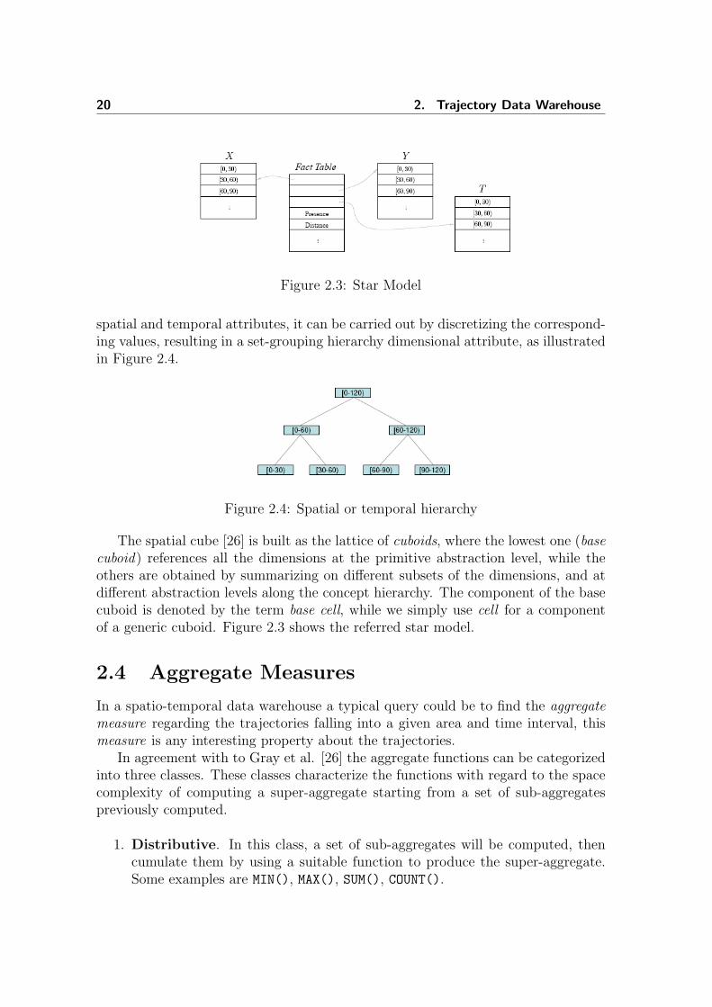
Figure 2.3: Star Model
spatial and temporal attributes, it can be carried out by discretizing the correspond-ing values, resulting in a set-grouping hierarchy dimensional attribute, as illustratedin Figure 2.4.
Figure 2.4: Spatial or temporal hierarchy
The spatial cube [26] is built as the lattice of cuboids, where the lowest one (basecuboid) references all the dimensions at the primitive abstraction level, while theothers are obtained by summarizing on different subsets of the dimensions, and atdifferent abstraction levels along the concept hierarchy. The component of the basecuboid is denoted by the term base cell, while we simply use cell for a componentof a generic cuboid. Figure 2.3 shows the referred star model.
2.4 Aggregate Measures
In a spatio-temporal data warehouse a typical query could be to find the aggregatemeasure regarding the trajectories falling into a given area and time interval, thismeasure is any interesting property about the trajectories.
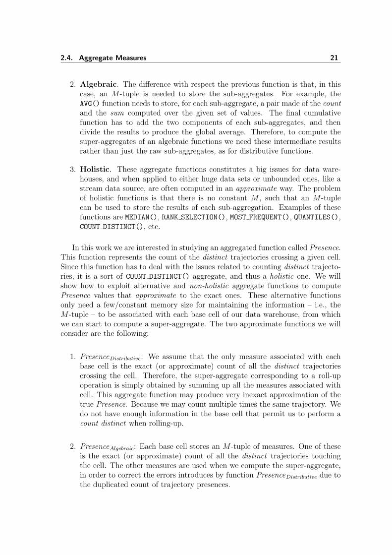
In agreement with to Gray et al. [26] the aggregate functions can be categorizedinto three classes. These classes characterize the functions with regard to the spacecomplexity of computing a super-aggregate starting from a set of sub-aggregatespreviously computed.
1. Distributive. In this class, a set of sub-aggregates will be computed, thencumulate them by using a suitable function to produce the super-aggregate.Some examples are MIN(), MAX(), SUM(), COUNT().
2.4. Aggregate Measures 21
2. Algebraic. The difference with respect the previous function is that, in thiscase, an M -tuple is needed to store the sub-aggregates. For example, theAVG() function needs to store, for each sub-aggregate, a pair made of the countand the sum computed over the given set of values. The final cumulativefunction has to add the two components of each sub-aggregates, and thendivide the results to produce the global average. Therefore, to compute thesuper-aggregates of an algebraic functions we need these intermediate resultsrather than just the raw sub-aggregates, as for distributive functions.
3. Holistic. These aggregate functions constitutes a big issues for data ware-houses, and when applied to either huge data sets or unbounded ones, like astream data source, are often computed in an approximate way. The problemof holistic functions is that there is no constant M , such that an M -tuplecan be used to store the results of each sub-aggregation. Examples of thesefunctions are MEDIAN(), RANK SELECTION(), MOST FREQUENT(), QUANTILES(),COUNT DISTINCT(), etc.
In this work we are interested in studying an aggregated function called Presence.This function represents the count of the distinct trajectories crossing a given cell.Since this function has to deal with the issues related to counting distinct trajecto-ries, it is a sort of COUNT DISTINCT() aggregate, and thus a holistic one. We willshow how to exploit alternative and non-holistic aggregate functions to computePresence values that approximate to the exact ones. These alternative functionsonly need a few/constant memory size for maintaining the information – i.e., theM -tuple – to be associated with each base cell of our data warehouse, from whichwe can start to compute a super-aggregate. The two approximate functions we willconsider are the following:
1. PresenceDistributive: We assume that the only measure associated with eachbase cell is the exact (or approximate) count of all the distinct trajectoriescrossing the cell. Therefore, the super-aggregate corresponding to a roll-upoperation is simply obtained by summing up all the measures associated withcell. This aggregate function may produce very inexact approximation of thetrue Presence. Because we may count multiple times the same trajectory. Wedo not have enough information in the base cell that permit us to perform acount distinct when rolling-up.
2. PresenceAlgebraic: Each base cell stores an M -tuple of measures. One of theseis the exact (or approximate) count of all the distinct trajectories touchingthe cell. The other measures are used when we compute the super-aggregate,in order to correct the errors introduces by function PresenceDistributive due tothe duplicated count of trajectory presences.
22 2. Trajectory Data Warehouse
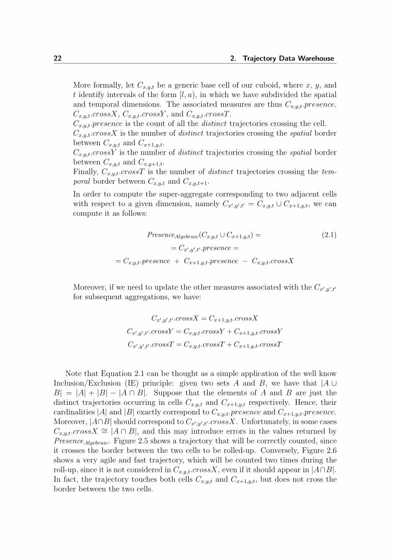
More formally, let Cx,y,t be a generic base cell of our cuboid, where x, y, andt identify intervals of the form [l, u), in which we have subdivided the spatialand temporal dimensions. The associated measures are thus Cx,y,t.presence,Cx,y,t.crossX, Cx,y,t.crossY , and Cx,y,t.crossT .Cx,y,t.presence is the count of all the distinct trajectories crossing the cell.Cx,y,t.crossX is the number of distinct trajectories crossing the spatial borderbetween Cx,y,t and Cx+1,y,t.Cx,y,t.crossY is the number of distinct trajectories crossing the spatial borderbetween Cx,y,t and Cx,y+1,t.Finally, Cx,y,t.crossT is the number of distinct trajectories crossing the tem-poral border between Cx,y,t and Cx,y,t+1.
In order to compute the super-aggregate corresponding to two adjacent cellswith respect to a given dimension, namely Cx′,y′,t′ = Cx,y,t ∪ Cx+1,y,t, we cancompute it as follows:
PresenceAlgebraic(Cx,y,t ∪ Cx+1,y,t) = (2.1)
= Cx′,y′,t′ .presence =
= Cx,y,t.presence + Cx+1,y,t.presence − Cx,y,t.crossX
Moreover, if we need to update the other measures associated with the Cx′,y′,t′
for subsequent aggregations, we have:
Cx′,y′,t′ .crossX = Cx+1,y,t.crossX
Cx′,y′,t′ .crossY = Cx,y,t.crossY + Cx+1,y,t.crossY
Cx′,y′,t′ .crossT = Cx,y,t.crossT + Cx+1,y,t.crossT
Note that Equation 2.1 can be thought as a simple application of the well knowInclusion/Exclusion (IE) principle: given two sets A and B, we have that |A ∪B| = |A| + |B| − |A ∩ B|. Suppose that the elements of A and B are just thedistinct trajectories occurring in cells Cx,y,t and Cx+1,y,t respectively. Hence, theircardinalities |A| and |B| exactly correspond to Cx,y,t.presence and Cx+1,y,t.presence.Moreover, |A∩B| should correspond to Cx′,y′,t′ .crossX. Unfortunately, in some casesCx,y,t.crossX ∼= |A ∩ B|, and this may introduce errors in the values returned byPresenceAlgebraic. Figure 2.5 shows a trajectory that will be correctly counted, sinceit crosses the border between the two cells to be rolled-up. Conversely, Figure 2.6shows a very agile and fast trajectory, which will be counted two times during theroll-up, since it is not considered in Cx,y,t.crossX, even if it should appear in |A∩B|.In fact, the trajectory touches both cells Cx,y,t and Cx+1,y,t, but does not cross theborder between the two cells.

2.5. Load Phase 23
Figure 2.5: Correctly counted Figure 2.6: Duplicate counting
2.5 Load Phase
The feeding of the data warehouse is a very important step in order to obtain correctresults using aggregate functions. The feeding begins at the base cells of the basecuboid, with suitable sub-aggregate measures, from which starting to compute super-aggregated functions. A stream of trajectory observations can arrive at differentrates and in an unpredictable and unbounded way. In this manner, is necessaryto limit the amount of buffer memory needed to store information about activetrajectories. The system module that is responsible for feeding data can consider atrajectory as inactive when, for a long time interval, no further observations relativeto a given object have been received. The inactive trajectories could be removedfrom the buffer, it is a manner to free memory space.
Figure 2.7: Linear interpolation
Figure 2.8: Interpolated trajectory(spatial-temporal points)
Some examples of sub-aggregate numeric measures to be stored in each base cell

24 2. Trajectory Data Warehouse
are:
1. number of observations;
2. number of trajectories, i.e., our Presence;
3. total distance covered by trajectories;
4. number of trajectories that covered a distance larger than a given d;
5. number of trajectories that followed a closed path, i.e., which started andended on the same point (with tolerance d).
Some measures require a pre-computation, and can be updated in the data ware-house as soon as single observations of the various trajectories arrive. We suggesta classification, ordering the measures according to an increasing amount of pre-calculation effort:
a) no pre-computation: the measure can be updated in the data warehouse bydirectly using each single observation;
b) per trajectory local pre-computation: the measure can be updated by exploitinga simple pre-computation, which only involves a few and close observations ofthe same trajectory;
c) per trajectory global pre-computation: the measure update requires a pre-computation which considers all the observations of each trajectory;
d) global pre-computation: it is required the complete re-computation of the ag-gregate on all the input raw data / trajectories. Thus, these measure cannotbe treated and computed by using a data warehouse.
Referring to the above examples, measure 1 is of type (a), while measure 2 isof type (b), even if in the experimental part we will try to threat it as a measureof type (a), thus introducing several errors in the sub-aggregates stored in the basecell of our data warehouse. Finally, measure 3 is of type (b), and measures 4 and 5are of type (c).
The amount of pre-computation associated with each type of measure impactupon the amount of memory required to buffer incoming trajectory observations.Measures of type (a) are the less expensive in terms of space and time, since it isenough to consider observations one at a time, without buffering anything. Thereforea measure can be updated as soon as each single observation Lj
i = (xji , yj
i , tji )of the various trajectories arrives. Conversely, for type (b) the measure must becomputed starting from a finite set of neighbors of each observation Lj
i = (xji , yj
i , tji ).For example, this could require a k-window of observations Lj−k−1
i , . . . , Lji to be
considered and stored in a buffer.

2.5. Load Phase 25
If we need to interpolate the observations to store correct measures in the basecells of our data warehouse, the aggregate measure we plan to compute should be, atleast, of type (b). As a matter of fact, when the observation Lj
i = (xji , yj
i , tji ) arrives,in order to interpolate, thus inferring the trajectory route, we have to maintainavailable in the buffer the previous trajectory observation Lj−1
i = (xj−1i , yj−1
i , tj−1i ).
Given the observations for a trajectory shown in Figure 2.2, a possible recon-structed trajectory using linear interpolation is shown in Figure 2.7, where we alsoillustrate the discretized 2D space.
If we updated the data warehouse on the basis of each single observation, themeasures (M1, . . . ,Mk), possibly corresponding to the four observations of our ex-ample, could naturally be stored in the following cells:
Time label X Y T M1 . . . Mk
10 [30,60) [30,60) [0,30) . . . . . . . . .65 [60,90) [30,60) [60,90) . . . . . . . . .75 [90,120) [90,120) [60,90) . . . . . . . . .120 [120,150) [90,120) [60,120) . . . . . . . . .
Table 2.1: Cells representation - for each observation
This approach will be correct only if consider measure is of type (a), otherwiseseveral errors will be introduced. Other cells might be crossed by the moving object,without reconstructing the full trajectory and adding further intermediate points,we are not able to store any information about the trajectory in these other cells.
(ti, ti+1) X Y T M1 . . . Mk
(10,30) [30,60) [30,60) [0,30) . . . . . . . . .(30,32) [30,60) [30,60) [30,60) . . . . . . . . .(32,60) [90,120) [30,60) [30,60) . . . . . . . . .(60,65) [90,120) [30,60) [60,90) . . . . . . . . .(65,67) [90,120) [30,60) [60,90) . . . . . . . . .(67,70) [90,120) [90,120) [60,90) . . . . . . . . .(70,73) [120,150) [90,120) [60,90) . . . . . . . . .(73,75) [120,150) [120,150) [60,90) . . . . . . . . .(75,90) [120,150) [120,150) [60,90) . . . . . . . . .(90,99) [120,150) [120,150) [90,120) . . . . . . . . .(99,120) [150,180) [120,150) [90,120) . . . . . . . . .
Table 2.2: Sequence of segments composing the interpolated trajectory, and the basecells that completely include each segment.
On the basis of the linearly interpolated trajectory of Figure 2.7, we can thus addfurther interpolated points for each cell crossed by a trajectory. We add points thatcross the borders of each crossed cell, considering all its three dimensions. The choice

26 2. Trajectory Data Warehouse
of adding all such intermediate points simplifies the computation of several measuresto associate with each base cell. Figure 2.8 shows the resulting interpolated pointsas white and gray circles. The white interpolated points, associated with temporallabels 30, 60, and 90, have been added to match the granularity of the temporaldimension. In fact, they correspond to cross points of a temporal border of some3D cell. The gray points, labeled with 32, 67, 70, 73, and 99, have been insteadintroduced to match the spatial dimensions. They correspond to the cross points ofthe spatial borders of some 3D cell, or, equivalently, the cross points of the spatial2D squares shown in Figure 2.8.
After the including of these additional interpolated points, we have further 3Dbase cells in which we can now store significant measures associated with the tra-jectory of the given object. The new points subdivide the interpolated trajectoryinto small segments, each one completely included in some 3D base cell. Thereforewe can now update a cell measure on the basis of a single trajectory segment. TheTable 2.2 shows the sequence of edges composing the interpolated trajectory of Fig-ure 2.8, and the base cell which the edge belongs to. For the sake of simplicity, eachedge is identified by a pair of timestamps (ti,ti+1), associated with the starting andending points.
2.6 Presence Measure
On Section 2.4 we defined two approximate aggregate functions we would like toexploit in order to approximate to the holistic aggregate Presence, namely Pres-enceDistributive and PresenceAlgebraic, of Presence, defined as as the number of distincttrajectories present in a given spatio-temporal cell.
In order to update the sub-aggregate measures stored in each base cell Cx,y,t,namely Cx,y,t.presence, Cx,y,t.crossX, Cx,y,t.crossY , and Cx,y,t.crossT , we have dif-ferent options.
1. single observations (type a). In this case we can only update/increment ameasure Cx,y,t.presence. Since we do not use any buffer, we cannot rememberthe previous points of each trajectory. Thus in this case we cannot updateCx,y,t.crossX, Cx,y,t.crossY , and Cx,y,t.crossT .
2. a pair of observations (type b). In particular, the currently received obser-vation Lj
i of trajectory Ti, along with the previous buffered Lj−1i one. Using
this pair of points, we can linearly interpolate the trajectory. If we buffer nononly the previous observation Lj−1
i , but also the last Cx,y,t.presence that wasmodified on the basis of Lt−1
i , we can avoid most of the duplicate presencecounts of trajectories when the two consecutive points fall in the same basecell.
Moreover, by exploiting linear interpolation, we can also identify the cross

2.6. Presence Measure 27
points of each base cell, and can accordingly update the various Cx,y,t.crossX,Cx,y,t.crossY , and Cx,y,t.crossT .
3. a window of k observations (type b). In particular, let Lji = (xj
i , yji , tji ) be the
currently received observation of trajectory Ti. The k window thus includesLj−k−1
i , Lj−k−2i , . . . , Lj−1
i , Lji . The window size k is dynamically adjusted
according to the following constraints: (1) All tj−k−1, . . . , tj must fall withinthe same temporal interval [l, u), characterizing a base cells of our cuboid.More formally, l ≤ tj−k−1 < tj−k−2 < . . . < tj < u. (2) In addition, Lj−k
i mustnot be included in the window, because tj−k < l.
Buffering all these points (and some related information) guarantees the linearinterpolation of the associated trajectory, and permits us to completely avoidduplicates when we update an aggregate measure Cx,y,t.presence. To thisend, it is enough to maintain the information about which are the cells whosepresence measures have been updated on the basis of the window points. Itis straightforward to show that if we encounter a new observation Lj+1
i , suchthat tj+1 ≥ u, we can forget (un-buffer) all the points of the window, since weare surely going to update new cells, associated with a different and successivetemporal interval.
Moreover, using the window of k points, we can also update Cx,y,t.crossX,Cx,y,t.crossY , and Cx,y,t.crossT without duplicates. For example, think abouta trajectory that, in the same base time interval, quickly goes ahead andback, crossing multiple times the same spatial border of two cells. By main-taining information about which measures have been updated on the basis ofthe window points, we can avoid these duplicate counts of the same crossingtrajectory.
Given the three methods for loading the base cell measures, the correspondingaggregate functions are:
1. single observations: We can use this loading method for approximating thepresence measures associated with each base cell. These approximate sub-aggregates can then be used by our distributive aggregate function, denotedas Presence1
Distributive. It is worth noting that we cannot exploit our aggregatealgebraic function (Presence1
Algebraic). This is because, using only single obser-vations, we cannot compute the counts of the trajectories crossing the bordersof the base cells.
2. observation pairs: We can use this loading method for approximating allthe needed measures associated with each base cell, both presence and crosscounts. These approximate sub-aggregates can then be used by our distribu-tive/algebraic aggregate functions, denoted as Presence2
Distributive and Pres-ence2
Algebraic.

28 2. Trajectory Data Warehouse
3. observation windows: We can use this loading method for exactly comput-ing all the needed measures associated with each base cell, both presence andcross counts. These exact sub-aggregates can then be used by our distribu-tive/algebraic aggregate functions, denoted as Presencek
Distributive and Pres-encek
Algebraic.
In the prototype we have used the method pair of observations in order toupdate the sub-aggregate measures for each cell.
2.7 The Prototype
We developed a prototype in order to implement the proposed TDW. The pro-totype can implement a TDW in agreement with the concepts presented in thesections above. Besides, the computation of aggregated measures and a mechanismto compute roll-up operations were implemented in the prototype. The TDW waspopulated by using the synthetic datasets generated by the traffic simulator de-scribed in [8]. The measures stored in the TDW can be used to discover interestingphenomena of the trajectories. The application tries to solve the both problems:loading and aggregation, which were presented in Sections 2.5 and 2.4.
Figure 2.9: Results Interface
Figure 2.9 shows the interface to visualize the values of the measures computedconsidering a cell selected by the user. The result presents the evolution of the valuesof measures in a range of time. In the same visualization is possible to define different

2.7. The Prototype 29
values of roll-up operations. The roll-up operation can be defined by the usage ofthe slider controls over the map, a more detailed explanation will be presented inthe next sections.
The TDW was implemented in a traditional data warehouse tool. We usedthe MS SQL SERVER 2005. The TDW was modeled in agreement with the starmodel [34]. We defined a fact table and three dimension tables (X and Y spatialdimensions and T temporal dimension). Tables 2.3, 2.4 and 2.5 present the structureof these tables (fact and dimensions). The level of granularity of the trajectory datawarehouse can be defined in the prototype. It allows to control the loading of theTDW and computation of the measures and aggregations. Each tuple stored inthe fact table represents a summarization of the measures that are delimited by theborders of the cell. The base cell are delimited by the tid, xid and yid values. Themeasures presented in Table 2.3 are detailed in Sections 2.5 and 2.4. The measurespresence, xborder, yborder and tborder are necessary in order to compute the holisticpresence measure. These measures are specially important when it is necessary tocompute the roll-up operations.
Table 2.3: Fact Tabletid time foreign keyxid X spatial foreign keyyid Y spatial foreign key
numobs Number of observations in the celltrajinit Number of trajectories starting in the cellvmax Maximum speed of trajectories in the cell
distance Total distance covered by trajectories in the celltime Total time spend by the trajectories in the cell
presence Number of trajectories in the cell - distributivexborder Number of trajectories crossing the x cell borderyborder Number of trajectories crossing the y cell bordertborder Number of trajectories crossing the t cell borderspeed Average speed of trajectories in the cell
Table 2.4: X or Y Dimension Tablexid primary keyxl1 first level of hierarchyxl2 second level of hierarchy
Table 2.5: T Dimension Tabletid primary keytl1 first level of hierarchytl2 second level of hierarchy
The prototype allows to set the environment in order to receive the data volume.It is done loading the data volume into a buffer table (see Table 2.6). Consideringthat the trajectory data are produced in an unpredictable and unbounded way, wehave to store data into a buffer table. This procedure allows to release space in thebuffer table. It can be done by the exclusion of the tuples of the ended trajectories.

30 2. Trajectory Data Warehouse
Table 2.6: Buffer Tableoid Object Identifier
xvalue X spatial valueyvalue Y spatial valuetvalue T time valuedift Time variation between two consecutive positionsdifx X spatial variation between two consecutive positionsdify Y spatial variation between two consecutive positionsdist Distance covered between two consecutive positionsvel Speed between two consecutive positions
idrow Identifier of the rowtimestamp Timestamp of the observation
Through the loader component it is possible to define some characteristics of theenvironment and to compute the interpolation procedure. In order to compute theinterpolation and to load the TDW two parameters must be defined: Granularitylevel and Dimension hierarchical level.
The definition of the granularity level is necessary to build the regular grid whichdivides the spatio-temporal environment. This procedure is done before the loadingthe TDW. After the definition of the granularity level it is possible to define thehierarchy level of the dimension tables. This procedure also can be done by theloader component.
Figure 2.10: Loading Settings
Figure 2.10 shows a visualization of the interface available to define those set-tings. These procedures are just executed once, before the beginning of the loadingthe data warehouse. After the definition of the settings explained above, the inter-

2.7. The Prototype 31
face allows to start the process for receiving the data stream values and loading theTDW.
Algorithm 1 presents the basic procedures to complete the loader process. Ccur
represents the current base cell, Cprev the previous base cell stored in the bufferrelated to the same trajectory, and IP represents the set of base cells computedby the interpolation process. Using the setting values already defined, the loadercomponent gets the active values in the buffer table and performs the procedures toload the TDW.
Algorithm 1 LoadingInput: {Stream SO of observations - id, x, y, t}Output: {Fact Table FT}FT ←− ∅buffer ←− ∅repeat
obs←− next(SO)Ccur ←− findCell(obs.x, obs.y, obs.t)if obs.id 6∈ buffer then
insertbuffer(obs.id)else
Cprev ←− findCell(obs.x, obs.y, obs.t)IP ←− interp(Ccur, Cprev)ct←− 1
end ifrepeat
if IP [ct] 6∈ FT theninsert(IP [ct], FT )
elseupdate(IP [ct], FT )
end ifct←− ct + 1
until ct < IP.numpointuntil
We described the concept of interpolation (see Section 2.5) used in order to loadthe TDW. The buffer table is used in order to implement that procedure. For eachactive row of the buffer table the application has to find the related cell in the TDW.If exists a row in the fact table for that cell, the values of distributive measures (e.gnumobs, trajinit) can be updated, otherwise a new row will be inserted in the facttable. It is the procedure when is not necessary to compute the interpolation.
When is necessary to compute the interpolation, the procedure must use theidentifier of the active trajectories, their last processed point, the cell such pointbelongs to, and the speed in the segment ending at such a point. Using that setof values it is possible to determine the additional points in order to represent the

32 2. Trajectory Data Warehouse
intersections among the trajectory and the borders of the cells. The additionalpoints can be computed considering the constant speed of the trajectory and thespatio-temporal granularity.
In Algorithm 1, the function interp computes the additional points of the inter-polation process. For each new point computed by the interpolation process it isexecuted a search to find the related cell in the TDW. Whether there is the base cellin the fact table, the related measures must be updated. Otherwise, the procedureis to insert a tuple with the new values of the measures.
In the prototype the pre-aggregated values are stored in the TDW. These pre-aggregated values are computed in the loading phase. However, when is necessaryto compute some query or to perform a roll-up operation, the application uses theaggregation component. Figure 2.9 shows the results of a query defined by theboundaries of the cell selected on the map. The results are represented by thecharts (right side) where it is possible to verify the evolution of the measures foreach value of time dimension. The user can choose the query base cell either bythe usage of the combo-boxes or by clicking on the map. The map is divided into aregular grid, this division is done in agreement with the granularity defined by theuser.
2.7.1 Assessments of the Prototype
In this section we present a report of the experiments in order to evaluate the TDWprototype. We conducted tests to measure the time taken for loading the TDWData Cube, and to measure the accuracy of the roll-up operations.
We conducted the tests using a TDW defined with three different values ofspatio-temporal granularity. The granularity was defined considering the length ofthe borders of the spatio-temporal cell. Table 2.7 presents the length values for eachborder of spatio-temporal cell.
Table 2.7: Spatio-temporal GranularityDimensions Length
Granularity X Y T125 G 125000 125000 10250 G 250000 250000 10500 G 500000 500000 10
For each level of granularity we computed roll-up operations (three levels: 1g, 2gand 3g) on the measure presence. We used traditional roll-up operations (summingup the sub-aggregate values) and our proposed model (algebraic presence). Eachresult obtained was compared with the correct values. We consider the number ofdistinct trajectories crossing the area as the correct value.

2.7. The Prototype 33
Error = 100 ∗ ‖C −R‖‖R‖
(2.2)
The error level was computed by using Equation 2.2. C represents the computedvalue and R the real value of distinct trajectories crossing the area.
Figures 2.11, 2.12 and 2.13 present the error values for each granularity along theroll-up levels. For all levels of granularity (125, 250 and 500 ) our proposal presentsthe lower level of error.
0
10
20
30
40
50
1 1.5 2 2.5 3
Err
or (
%)
Rollup Level
Error Rollup Presence: Algebraic vs Distributive - Granularity 125
AlgebraicDistributive
Figure 2.11: Granularity 125
0
10
20
30
40
50
1 1.5 2 2.5 3
Err
or (
%)
Rollup Level
Error Rollup Presence: Algebraic vs Distributive - Granularity 250
AlgebraicDistributive
Figure 2.12: Granularity 250
Also it is possible to verify that the level of error of our proposal remains almoststable along the roll-up level (1g, 2g and 3g). The error level of the distributivemodel decreases while the level of granularity increases. It can be explained by the

34 2. Trajectory Data Warehouse
0
10
20
30
40
50
1 1.5 2 2.5 3
Err
or (
%)
Rollup Level
Error Rollup Presence: Algebraic vs Distributive - Granularity 500
AlgebraicDistributive
Figure 2.13: Granularity 500
fact that the number of trajectories crossing a base cell decreases in agreement withthe growth of the granularity level.
In order to measure the time taken to load the cube, we simulated several datavolumes of stream observations, with different number of observations for each ofthem. For each data volume, it was verified the ratio between the time taken to loadthe observations into the cube, and the number of observations. In the loading weconsider the loading of the buffer table, the computation of the interpolated points,the computation of the sub-aggregate measures and the consequent loading to thedata cube.
Tobs =Ttot
Nobs
(2.3)
Thr =1
Tobs
(2.4)
The time taken to load the cube, by observation, was computed by Equation2.3. Ttot represents the total time considering the receiving, interpolation and com-putation of the sub aggregates values. Nobs represents the number of observationsloaded. The throughput (Thr) is computed by Equation 2.4 and it represents thenumber of observations loaded into the cube by second.
Figure 2.14 presents the results of this test expressed in seconds / number ofobservations. We considered several data sets composed by 21017, 39208, 62219,107865 and 156113 observations. The time taken to load the cube is stable, itremains in the same level (Tobs
∼= 0.005 seconds/observation - Thr ∼= 200) for allthe different packages of observations.

2.8. TDW: Events Occurrences Patterns 35
0
2
4
6
8
10
20000 40000 60000 80000 100000 120000 140000 160000
Rat
io: t
ime(
ms)
/obs
erva
tions
Number of Objects
Time (milliseconds) / Observations
Figure 2.14: Loading
2.8 TDW: Events Occurrences Patterns
In this section we perform some statistical analysis on the data stored in the variouscells, to discover correlation in such data. The statistical analysis was conducted byusing the Pearson correlation index. Besides, we investigate the use of traditionaldata mining techniques to reveal patterns of occurrences of events. We focus on atraffic jam occurrence. It was done adding supervised knowledge to data recordsassociated with cells, by labeling them with respect to the occurrence of a trafficjam phenomena, and then investigating whether it is possible to extract good (clas-sification) models from all the labeled records associated with the cells. The goal isto verify whether it is possible conclude something about the occurrence of a TJ ina spatio-temporal cell by only looking at the measures stored in the cells.
We consider a set of objects moving in a network, abstracted by an undirectedgraph. The area is divided into a regular grid, composed of a set of cells delimited by(x,y,t) spatio-temporal coordinates. In this environment a singular cell may involveseveral different edges, each of them presenting different characteristics. For exam-ple, consider a given cell involving six edges: three edges are considered crowded,while the three other ones are not crowded. In this case, what is the most adequaterepresentation of a TJ occurrence for that cell? In the following section we present aproposal to solve this problem. We argue that by using this model (an area dividedinto a regular grid, composed of a set cells) also is possible to individualize singularedges. It can be done defining an adequate level of granularity of the cells. In this

36 2. Trajectory Data Warehouse
way it is possible to investigate movement occurrences at individual edges and in anarea composed of different edges. We expect to obtain best results of precision in theanalysis of the events occurrences patterns by using low levels of granularity. Highlevels of granularity may involve a high number of different edges (with differentcharacteristics), therefore the accuracy of the results tends to decrease.
The most part of the section itself is concerned with the labeling of the cells. Itwas done because the use of a simulator to generate the dataset. By using a simula-tor, it is possible to manipulate some variables in order to generate an environment.Therefore, the cells were labeled considering the results of the simulator. In realenvironments, maybe it is possible to know from external sources whether an event(a Traffic Jam in this case) occurred (or not) in a given cell. In the following wepresent some details about the experiments and the obtained results.
2.8.1 Traffic Jam Patterns on TDW
We are interested in the investigation of the use of the aggregate measures storedin our TDW to discover the occurrence of specific phenomena. Actually, in thissection we consider a Traffic Jam occurrence. We have used the fact table rows [7]in order to mine patterns revealing TJ. Table 2.11 shows the measures that we haveconsidered to complete this experiment. Each fact table row stores the summarizedvalues of measures for a given cell (x,y,t).
Our goal is to use a classification mining task in order to extract a classificationmodel able to reveal TJ occurrences. The TDW fact table rows were labeled torepresent the occurrence of a TJ phenomenon for each cell(x,y,t).
In order to solve the problem introduced in the last section (a same cell composedof several different edges) we have proposed to measure the TJ occurrence with avalue that represents the density of TJ occurrences for each cell. Equation 2.5was defined in order to compute the TJ density value (dTJx,y,t) for each cell(x,y,t).NedTJx,y,t represents the number of edges labeled with Crowded=Yes for a givencell(x,y,t), and Nedx,y,t represents the number of edges involved by cell(x,y,t).
dTJx,y,t =NedTJx,y,t
Nedx,y,t
(2.5)
The value of dTJx,y,t represents the probability of the occurrence of a trafficjam phenomenon in a given cell(x,y,t). The measure dTJx,y,t is not available in theTDW. We have used it to label TDW cells, thus preparing a training set for theclassification method. The goal of the experiment is to confirm the our proposal toidentify a serious Traffic Jam phenomenon in our TDW :
A traffic jam occurrence can be identified by the simultaneous occurrence of the twoconditions in the measures stored in the TDW:
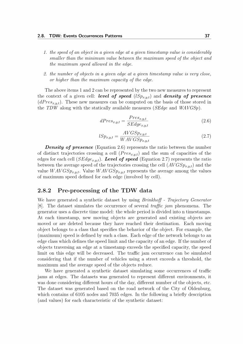
2.8. TDW: Events Occurrences Patterns 37
1. the speed of an object in a given edge at a given timestamp value is considerablysmaller than the minimum value between the maximum speed of the object andthe maximum speed allowed in the edge.
2. the number of objects in a given edge at a given timestamp value is very close,or higher than the maximum capacity of the edge.
The above items 1 and 2 can be represented by the two new measures to representthe context of a given cell: level of speed (lSpx,y,t) and density of presence(dPresx,y,t). These new measures can be computed on the basis of those stored inthe TDW along with the statically available measures (SEdge and WAVGSp).
dPresx,y,t =Presx,y,t
SEdgex,y,t
(2.6)
lSpx,y,t =AV GSpx,y,t
WAV GSpx,y,t
(2.7)
Density of presence (Equation 2.6) represents the ratio between the numberof distinct trajectories crossing a cell (Presx,y,t) and the sum of capacities of theedges for each cell (SEdgex,y,t). Level of speed (Equation 2.7) represents the ratiobetween the average speed of the trajectories crossing the cell (AV GSpx,y,t) and thevalue WAV GSpx,y,t. Value WAV GSpx,y,t represents the average among the valuesof maximum speed defined for each edge (involved by cell).
2.8.2 Pre-processing of the TDW data
We have generated a synthetic dataset by using Brinkhoff - Trajectory Generator[8]. The dataset simulates the occurrence of several traffic jam phenomena. Thegenerator uses a discrete time model: the whole period is divided into n timestamps.At each timestamp, new moving objects are generated and existing objects aremoved or are deleted because they have reached their destination. Each movingobject belongs to a class that specifies the behavior of the object. For example, the(maximum) speed is defined by such a class. Each edge of the network belongs to anedge class which defines the speed limit and the capacity of an edge. If the number ofobjects traversing an edge at a timestamp exceeds the specified capacity, the speedlimit on this edge will be decreased. The traffic jam occurrence can be simulatedconsidering that if the number of vehicles using a street exceeds a threshold, themaximum and the average speed of the objects reduce.
We have generated a synthetic dataset simulating some occurrences of trafficjams at edges. The datasets was generated to represent different environments, itwas done considering different hours of the day, different number of the objects, etc.The dataset was generated based on the road network of the City of Oldenburg,which contains of 6105 nodes and 7035 edges. In the following a briefly description(and values) for each characteristic of the synthetic dataset:

38 2. Trajectory Data Warehouse
• 73520 Moving Objects is the number of objects traveling on the network;
• 657281 Points represents the number of positions reported in the dataset;
• 2592445 Traversed Nodes is the number of nodes traversed by objectstraveling on the network;
• 74483 Routes represents the number of routes 1 defined in the simulation;
• 5789 AVG route length represents the average length of the routes.
For generated dataset we have studied the logs created by the simulator. Wehave modified the simulator to include new attributes into the original log: Edge id,Edge Capacity and Maximum Speed. It was done in order to investigate the trafficjam occurrence. The synthetic dataset was generated considering that a traffic jamhappens when the number of objects traversing an edge at a timestamp exceeds itscapacity [8]. Therefore, by using the additional information (edge id, edge capacity,maximum speed) we can identify an occurrence of traffic jam: where (edge) and when(timestamp) it occurs. Table 2.8 presents the attributes of the log of the generateddataset.
Table 2.8: Trajectories LogAttribute Description
Status Status of pointId Identifier of pointSeq Sequence number
Class Object Id Identifier of objects classTime Timestamp
X X-coordinateY Y-coordinate
Speed Current speed of objectEdge Id Identifier of the edge
Edge Capacity Max. capacity of objectsSpeed Maximum Max. speed in the edge
The counting of the different objects by grouping by Edge Id (Identifier of theedge) and Time (timestamp) allows to identify the edges and timestamps where atraffic jam phenomenon may be happened. The following SQL expression was usedin our experiments in order to identify the possible occurrences of traffic jam.
Select EdgeID, Timestamp, Count(ID) From TrajectoryLog
Group By EdgeID, Timestamp
Having Count(ID) >= EdgeCapacity
1Each object obj moves between two timestamps ti and ti+1 from its current position obj.loci
to its new position obj.loci+1 according to its computed route

2.8. TDW: Events Occurrences Patterns 39
The SQL expression only uses the edge capacity as constraint to select the recordswhose a traffic jam is likely happening. It was done because it is the only methodto simulate a traffic jam occurrence by using the simulator.
The result set of the SQL expression allows us to label the records of the gener-ated dataset in which a traffic jam (TJ ) is likely happening. Table 2.9 describes theadditional attributes inserted in the Log Table in order to compose the Labeled LogTable. We have added the binary attribute Crowded to represent the situation ofthe capacity of the edge. A record whose the number of trajectories crossing the edgeis above the value of the maximum capacity of the edge will be represented by Yesvalue, the other records will be labeled with the value No. Therefore, the recordsobtained considering the True value of the above SQL predicate were labeled withYes value (Crowded attribute), and the other records are labeled with No value.
Table 2.9: Labeled TableAttribute Description Values
Class Class of Moving Object {0, 1, 2, 3, 4, 5}Cap Capacity Of Edge {1, 2, 3, 4, 5}
Crowded Situation of capacity of Edge {Yes, No}
We have defined different levels of TJ occurrence classified according to dTJx,y,t
value (see Equation 2.5), each of them representing a kind of density of TJ (con-sidering the number of edges involved in the cell). In this manner a given cell maybe classified into a TJ class in a given timestamp and to evolve in this classificationalong the time dimension.
Table 2.10: TJ Density DiscretizationDensity Range Label
[0, 0.25) 025TJ[0.25, 0.50) 050TJ[0.50, 0.75) 075TJ[0.75, 1.00] TJ
We have implemented a discretization process of the range of TJ density values.It was done to facility the classification mining task, Table 2.10 presents the levelsof TJ density discretization.
We have presented our proposal to identify a Traffic Jam phenomenon consid-ering the speed of the objects and the number of objects occurring during a giventimestamp (see Section 2.8.1). We have prepared two subsets in order to investigatethat proposition. The first one is the full dataset, composed of all attributes (seeTable 2.11), and the second subset was composed just using two new attributes usedto compute two new measures to represent the context of the cell:
We have discretized the complete range of the values of dPresx,y,t and lSpx,y,t.It was done to facilite the discovery of the patterns, it considers each interval of

40 2. Trajectory Data Warehouse
Table 2.11: Training Set SchemeSet 1 Set 2 Attribute Desciption• Disc numobs Discretized ] of observations• Disc trajinit Discretized ] of trajectories starting• Disc presence Discretized ] of trajectories• Disc time Discretized ] time taken• Disc distance Discretized Total distance covered by trajectories• Disc speed Discretized Average speed of trajectories• Disc vmax Discretized Maximum speed of trajectories• Disc acceleration Discretized Acceleration of trajectories crossing the cell• Disc Sum Edges Capacity Sum of the capacities of the edges• Disc Avg Edges Capacity Average of the capacities of the edges
• Disc dPres Discretized Density of Presence• Disc lSp Discretized Level of Speed
• • Label Discretized Density Range
discretization as an item in a frequent pattern processing.
2.8.3 Statistical Analysis
In this experiment we have used a dataset generated by the simulator, not a realdataset produced by a set of moving objects. Therefore, we expect that the syn-thetic dataset presents a behavior similar to a real environment. A possible way toinvestigate this behavior it is to compute the relationship among the measures. Apopular statistical measure to find the level of relationship between two measures itis the correlation. Besides, correlation can be used to investigate co-occurrence ofmeasures in cells. It is a very important point in order to verify whether it is possibleto conclude something about the occurrence of a event (TJ ) in a spatio-temporalcell by only looking at the measures stored in the cells.
In this section we present the results of a statistical analysis by using the completesynthetic dataset. We consider the relationship among the measures distance, time,dPres and lvlSpeed. We used the correlation value in order to identify the possiblerelationships. It is evident that the correlation among the measures can be influencedby several features. Dataset, road network and base granularity of the cells are someof the possible characteristics.
The Pearson coefficient is a measure statistic which estimates the correlationof the two given random variables. The coefficient values ranges from -1 to 1. Avalue of 0 shows that there is no linear relationship between the variables. A valueof 1 shows that there is a positive linear relationship between the variables. Whenthe Pearson coefficient is -1 it represents that there is a negative linear relationshipbetween the variables. Table of critical values for Pearson correlation was used toverify the correlation among the measures.

2.8. TDW: Events Occurrences Patterns 41
Table 2.12 presents the results of Pearson coefficient. By using the Table ofcritical values for Pearson correlation, it is possible to conclude that there is asignificative linear correlation among the measures. In the following we discuss theresults, the dispersion graphs are also presented for each relationship.
Table 2.12: Correlation - Pearson coefficientTime Distance dPres lvlSpeed
Time 1Distance 0.917 1dPres 0.438 0.551 1
lvlSpeed -0.318 -0.277 -0.113 1
[Time vs Distance] and [Time vs dPres] (Figures 2.15 and 2.16) are con-sidered positive linear relationships. Measure Time represents the time taken bytrajectories into the cell. This relationship suggests that when the trajectories re-main into the cell for a large time, the distance traveled by trajectories also willincrease. A similar behavior is observed between Time and Presence. When thenumber of distinct trajectories into a cell increase, it results in an increase in thetime taken by the trajectories. Those relationships may reveal a behavior similarto a real environment. Large cells containing roads that allow objects to move bystaying in the same cell it is an example of a real environment where those relation-ships could be found. Another possibility is an environment with a large number ofobjects, in this case the individual trace of each object can contribute to improvethe distance traveled by the complete set of objects.
0
10
20
30
40
50
60
70
80
0 5000 10000 15000 20000 25000 30000 35000 40000 45000 50000
Figure 2.15: Correlation Time vs Dis-tance
0
2
4
6
8
10
12
14
16
0 10 20 30 40 50 60 70 80
Figure 2.16: Correlation Time vsdPres
[Time vs lvlSpeed] (Figure 2.17) represents a moderate negative linear rela-tionship. In this case, the level of speed decreases when happen an increase in the

42 2. Trajectory Data Warehouse
time taken by the trajectories. This behavior can be explained considering the rela-tionship between time and presence. An increase in the time results in a consequentincrease in the number of distinct trajectories into the cell, it contributes to improvethe probability of occurrence of a traffic jam and, consequently, decreases the level ofspeed into the cell. Another evident cause of this relationship could be a cell crossedby a lot of very agile objects. In this case, the objects cross the borders of the cellwithout any occurrence of traffic jam. The consequence will be the reduction in thetime taken by the objects into the cell.
0
1
2
3
4
5
6
7
8
0 10 20 30 40 50 60 70 80
Figure 2.17: Correlation Time vs lvlSpeed
[Distance vs dPres] (Figure 2.18) is considered a strong positive linear rela-tionship. When the number of distinct trajectories increase, the same behavior canbe expected to the distance traveled by the trajectories into the cell. In this case,the behavior describes a cell with a large number of distinct trajectories. However,in this situation, the number of distinct trajectories is not sufficient to start a trafficjam phenomenon.
0
2
4
6
8
10
12
14
16
0 5000 10000 15000 20000 25000 30000 35000 40000 45000 50000
Figure 2.18: Correlation Distance vs dPres
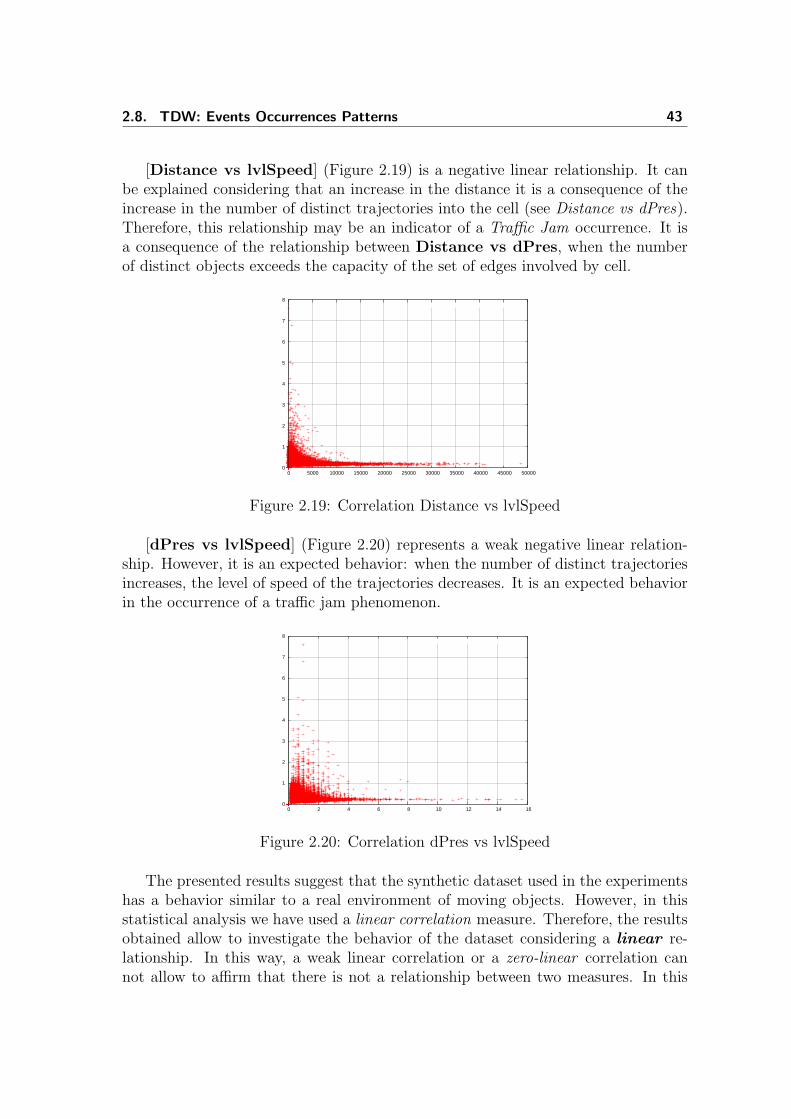
2.8. TDW: Events Occurrences Patterns 43
[Distance vs lvlSpeed] (Figure 2.19) is a negative linear relationship. It canbe explained considering that an increase in the distance it is a consequence of theincrease in the number of distinct trajectories into the cell (see Distance vs dPres).Therefore, this relationship may be an indicator of a Traffic Jam occurrence. It isa consequence of the relationship between Distance vs dPres, when the numberof distinct objects exceeds the capacity of the set of edges involved by cell.
0
1
2
3
4
5
6
7
8
0 5000 10000 15000 20000 25000 30000 35000 40000 45000 50000
Figure 2.19: Correlation Distance vs lvlSpeed
[dPres vs lvlSpeed] (Figure 2.20) represents a weak negative linear relation-ship. However, it is an expected behavior: when the number of distinct trajectoriesincreases, the level of speed of the trajectories decreases. It is an expected behaviorin the occurrence of a traffic jam phenomenon.
0
1
2
3
4
5
6
7
8
0 2 4 6 8 10 12 14 16
Figure 2.20: Correlation dPres vs lvlSpeed
The presented results suggest that the synthetic dataset used in the experimentshas a behavior similar to a real environment of moving objects. However, in thisstatistical analysis we have used a linear correlation measure. Therefore, the resultsobtained allow to investigate the behavior of the dataset considering a linear re-lationship. In this way, a weak linear correlation or a zero-linear correlation cannot allow to affirm that there is not a relationship between two measures. In this

44 2. Trajectory Data Warehouse
case, a non linear correlation could be found between the variables. However, in thisexperiment we consider enough to focus on linear correlation.
Besides, the statistical analysis allows to conclude that it is possible to use theco-occurrence of measures in spatio-temporal cells in order to investigate the a givenmovement event. However, it is not sufficient in order to conclude a relationshipamong measures and occurrences. It is only a step in this process that must becomplemented with additional techniques (e.g. supervised knowledge).
2.8.4 Data Mining Experiment Results
Classification was the data mining task used to conduct the tests. Test set valueswere obtained after a discretization process executed on the measures of the facttable rows (see Table 2.11). The goal is to verify if is possible to obtain a high levelof accuracy to foresee a Traffic Jam occurrence by using the new proposed measures(dPresx,y,t and lSpx,y,t).
The experiment was conducted by using the Weka suite, it is a data miningenvironment which offers several data mining tasks with various algorithms. Wehave used the classification mining considering three algorithms: ID3, BayesNetand J48. It was done in order to analyze the results independently of the algorithm.
Table 2.13 presents the results obtained with the experiment, it represents thevalues obtained considering the complete set of density of traffic jam values: {025TJ,050TJ, 075TJ, TJ}. Column Set shows the datasets detailed in Table 2.11 and Timecolumn presents, in seconds, the time to build the mining model. Column Instancesshows the percentage of instances Unclassified, Correctly and Incorrectly classified.Finally, column Precision presents the percentage of the accuracy for each level ofdensity of traffic jam.
Table 2.13: Accuracy Results (025TJ, 050TJ, 075TJ, TJ)Instances Precision
Algorithm Set Time Correct Incorrect Unclassified 025TJ 050TJ 075TJ TJID3 1 0.09 53.02% 43.630% 3.34% 61.70% 17.00% 27.70% 59.20%ID3 2 0.00 62.51% 37.35% 0.13% 66.30% 0.00% 45.50% 60.40%
BayesNet 1 0.08 58.22% 41.77% 0.00% 70.40% 17.60% 33.60% 64.70%BayesNet 2 0.00 61.29% 38.71% 0.00% 67.00% 0.00% 41.70% 58.20%
J48 1 0.16 61.15% 38.84% 0.00% 68.10% 20.00% 36.50% 62.20%J48 2 0.02 62.55% 37.44% 0.00% 66.40% 0.00% 41.70% 60.50%
The first point to analyze is the time to build the mining model, by using theset 2 (just dPresx,y,t and lSpx,y,t measures) we can obtain a significant reduction inthe value of the time independently of the algorithm . The same reduction can beobserved considering the value of the instances unclassified, the value is very closeto 0.00% in both cases (Set 2 ). In the same way, we can observe an increasing in thepercent of instances correctly classified. The value of instances incorrectly classified

2.8. TDW: Events Occurrences Patterns 45
also decreases for the two sets. In resume, by using the set 2 we have observed anincreasing of the accuracy to classify the instances. We have obtained this gain inthe same time that we have obtained an increase in the performance to build themodel.
About precision, we can observe that the best values happen in the 025TJ andTJ values of the density of traffic jam. In the intermediate values (050TJ and075TJ ) we did not obtain a reasonable accuracy. In the same way that happenedin the analysis of the classification of the instances, in the precision measure we canobserve an increase in the accuracy of the results by using the set 2. Similarly, thisgain happened with the reduction of the time to build the model.
Another point to analyze it is related to the rules produced by decision tree basedmining techniques. The set of trees produced by using the Set 1 as data source iscomposed of the attributes (see Table 2.11) Disc presence, Disc distance, Disc speed,Disc vmax, Disc acceleration and Disc Sum Edges Capacity. The number of levels ofthe trees, produced by Set 1, ranges between 5 and 6 levels. Meanwhile, the numberof levels of the all trees produced by using the Set 2 is 2 (Disc dPres, Disc lSp) .By using a number significantly smaller of tree levels it is possible to obtain betterresults, considering the accuracy of the foresee of the traffic jam event.
We have done another experiment by using the Set 1 in order to verify the distri-bution of the data regarding the threshold values defined as density of presence(dPresx,y,t) and level of speed (lSpx,y,t). By using the results obtained with thedata mining experiments, we have plotted the Figures 2.21 and 2.22.
0
10
20
30
40
50
60
70
80
90
100
0 0.25 0.5 0.75 1
Num
ber
of C
ells
(%
)
Density of Traffic Jam
density of presence <= 0.20 and level of speed >= 0.80
Figure 2.21: Number of Cells (%) vs TJ Density - Free Traffic
The results confirm that when the density of presence <= 0.20 and levelof speed >= 0.80, a typical environment of Free Traffic, 100% of the cells areclassified in the 025TJ. Similarly, when the density of presence >= 0.80 andlevel of speed <= 0.20, a typical environment of Traffic Jam, almost 80% of thecells are classified in the TJ. These thresholds are efficient to identify a traffic jam

46 2. Trajectory Data Warehouse
occurrence in a given cell. More than 80% of the objects are selected consideringthese values.
0
10
20
30
40
50
60
70
80
90
100
0 0.25 0.5 0.75 1
Num
ber
of C
ells
(%
)
Density of Traffic Jam
density of presence >= 0.80 and level of speed <= 0.20
Figure 2.22: Number of Cells (%) vs TJ Density - Traffic Jam
2.9 Conclusions
Our TDW offers an environment to receive, process and store trajectory data byusing the multidimensional concept. We proposed a data warehouse based on starschema: one fact table and three dimension tables. Each fact table record store mea-sures representing characteristics of a set of trajectories involved by cell coordinates(dimension tables).
We consider that the TDW works on a data stream environment. Therefore, theTDW must be able to offer a solution adequate to the data stream characteristics.The proposed TDW introduces measures and techniques of loading and aggregationconsidering the data stream environment.
In order to investigate the TDW, we developed and implemented a prototype.The prototype considers the constraints to load the data warehouse and computethe aggregation values. The application is a first step in order to solve the problemsof loading and aggregation in a TDW environment. The data cube model adoptedis very simple, it is just a contribution in order to improve the discussion aboutthe problems to implement a TDW. However, this model can be extended to moregeneral situations.
The current stage of the prototype can solve some problems of a trajectorydata warehouse environment. A possible future work may be to sophisticate thehierarchy of the dimensions. The loading phase is an opened problem. We limited

2.9. Conclusions 47
the loading phase considering a linear interpolation. However, it is possible to findsome topological situations (e.g roads, bridges) where the proposed interpolation isnot efficient, because of the some constraints in the movement of the object.
In this work we used the roll-up operation. However, may be interesting to offermechanisms in order to compute other operators such as drill-down, pivot, slice anddice. Therefore, the development of a query language using OLAP operators also isa possible point to research.
The results obtained in the experiments allow to consider the measures densityof presence and level of speed enough to investigate the occurrence of TJ events.The best results of accuracy (classification of instances) and precision (TJ densitylevels) were obtained in the Set 2 (density of presence and level of speed).Besides, the time taken to compute these patterns are also reduced by using the Set2. Therefore, considering the Traffic Jam event, the proposed TDW can be used toidentify occurrences in an environment of trajectories.
We have obtained a high level of accuracy to find TJ occurrences considering thecells whose level of traffic jam is 025TJ or TJ. Therefore, a possible future researchmay be to investigate new methods/algorithms to improve the accuracy of resultsanalyzing mixed cells.
The results of the statistical analysis (correlation) suggest that it is possible toinvestigate the use of co-location patterns among the measures of the TDW. Theproposal is to use the co-location patterns to investigate the occurrence of movementevents inter-region . In other words, an occurrence of an event (composed of asubset of measures) at a given area (region) could affect the occurrence of a differentconsequent event in another different area. The second part of this Thesis is focusedin this investigation, the goal is to verify whether traditional data mining techniquescan be used to reveal the hidden knowledge on trajectory data.

48 2. Trajectory Data Warehouse

IISecond Part

3Pattern Mining applied to
Trajectories
The development of new technologies for mobile computation and remote sensorsneed huge databases to store the data received concerning multitude of sampledmoving objects. Basically, in the most of the cases, the data report the location(2-dimensional space) of an object at a given timestamp. Therefore, by using therecords it is possible to reconstruct the trajectory of a moving object, even if somelevel of uncertainty in the reconstruction may occur. These trajectory databasescan be the source to discover a very important knowledge about moving objects:movement patterns.
There are a lot of environments where this knowledge can be applied: man-agement of road traffic, monitoring of movement of animals in order to investigatethe migratory phenomenon, air traffic, enemy movement in a battlefield and manyothers. In this chapter we present the related work to investigate the movementpatterns, all of them are based on a trajectory database to store the trajectory data.The goal is to discuss the requisites of a mechanism to find spatio-temporal patternson Trajectory DataWarehouse data. We focus on co-location patterns.
3.1 General Framework
On [57] the authors present a discussion about the use of data mining techniquesto find interesting spatio-temporal patterns from Earth Science data. In that work,the data consist of time series measurements for various Earth science and climatevariables (e.g. soil moisture, temperature and precipitation), along with additionaldata from existing ecosystem models. Those measurements represent a knowledgerelated to a given region. The presented environment has some similarities with theenvironment of TDW. In both environments we have a spatio-temporal area dividedinto a set of grid cells, and for each cell there is a set of measures representing char-acteristics of that region. As in the TDW environment, the ecologists are interestedin a variety of spatio-temporal association patterns involving sequences of eventsabstracted from the measures stored at each cell. The authors present four types ofpatterns: Intra-zone non sequential patterns , Inter-zone non-sequential
52 3. Pattern Mining applied to Trajectories
pattern , Intra-zone sequential pattern and Inter-zone sequential pattern .We argue that those patterns can be applied on the TDW environment. In the fol-lowing we present a description of those types of patterns and a possible frameworkof use of the concepts applied to trajectories.
3.1.1 Intra-zone non sequential patterns
By using this pattern the goal is to find relationships among events in the samecell (or set of cells), ignoring the temporal aspects of the data. Association rulemining algorithms (e.g Apriori [2]) could be used to reveal intra-zone non-sequentialassociations among events occurring at the same spatial location. In our TDW,each record can be considered as a transaction identified by cell coordinates. Therecords are composed of different items (discretized measures). Therefore, on a TDWenvironment an association rule antecedent→ consequent represents a relationshipamong discretized values of measures. This type of pattern may reveal differentrelationships among measures at different locations. The following association rulesare examples of possible patterns.
• (Area A) - 10densitypresence→ 01levelSpeed
• (Area B) - 10levelspeed→ 01time, 01densitypresence
The rules reveal two different behaviors. The rule found at area A representsa possible occurrence of a traffic jam event. When the number of distinct objectsincreases, the level speed of them decreases. However, the rule at area B representsan opposite situation, when the level speed of the objects is high, the value of timespent by the objects in that area is low, and the value of the density of presenceis also low. It may represent the behavior of fast objects crossing areas with highcapacity of traffic.
Therefore, this type of pattern can identify interesting behavior of moving objectsat a given area by using the traditional mining algorithms (Apriori, for example).However, we can not observe the evolution of the behavior along the time, and it isa crucial knowledge when the goal is to mine trajectories of moving objects.
3.1.2 Intra-zone sequential patterns
Temporal relationships among events occurring within the same cell. In this type ofpattern the temporal information is used to reveal the evolution of the behavior. Thetime dimension allows to find intra-zone sequential associations among the events.Traditional algorithms to find frequent sequential patterns in market-basket data canbe used in this case. In [3] the authors consider a database of sequences, where eachsequence is a list of transactions ordered by transaction-time, and each transactionis a set of items. The goal is to discover all sequential patterns with a user-specifiedminimum support, considering time constraints that specify a minimum and/or

3.1. General Framework 53
maximum time period between adjacent elements in the pattern. The support of apattern is the number of data-sequences that contain the pattern. In the same work([3]) the authors propose to relax the restriction that establishes that the items inan element of a sequential pattern must come from the same transaction. Instead,allowing the items to be present in a set of transactions whose transaction-times arewithin a user-specified time window.
The problem of finding sequential patterns in a database of sequences it is similarto the problem of finding sequential patterns of events in a TDW. The TDW recordscan be considered as transactions. Each of them identified by the cell coordinates.The discretized measures are the items of transaction. Therefore, an occurrence ofan event of movement may be represented by a sequence of discretized measures.
For example, an event of traffic jam may be represented by a sequence like〈10dpresence, 10time, 01levelspeed〉, where 10dpresence represents a high level ofdensity of presence, 01levelspeed represents a low level of speed of the objects and10time represents a high level of time spent by the trajectories into the cell.
Also on a TDW there is a time constraint which can be used to restrict thepatterns. In a TDW environment a time constraint may be the definition of amaximum time interval between successive elements in the sequence.
The sequential pattern 〈10dpresence, 01levelspeed, 10time〉 may not be enoughto represent the occurrence of a traffic jam event. We do not have the time infor-mation between the events. Therefore, the sequential pattern〈10dpresence, (5 minutes), 10time, (10 minutes), 01levelspeed〉 represents the eventmore precisely. In this case, the sequence pattern represents a traffic jam consider-ing a time-window of 15 minutes. However, by using a time-window of 10 minutes,the same sequence pattern does not represent a traffic jam event.
This type of pattern allows to reveal sequence patterns by using a time constraint.In a TDW environment it represents a useful knowledge to understand the evolution(creation, stabilization and dissipation) of the movement events.
3.1.3 Inter-zone non-sequential patterns
This pattern reveals the relationships among events happening in different cells,ignoring temporal aspects of the data. In a TDW environment it allows to in-vestigate whether the occurrence of an event at a given area can be related withthe occurrence of another event at a different area. In [54] the authors introducespatial co-location rules based on the frequent co-occurrences of events within thesame spatial window. However it is not possible to investigate how this relationshipdevelops along the time. In an environment of TDW the temporal dimension is avery important characteristic. We have to be able to identify the relationship amongthe occurrences of events at different areas. However, we also have to know how ithappens along the time. It is a crucial knowledge to forecast the occurrence of someevents (e.g. traffic jam) and to manage the environment.

54 3. Pattern Mining applied to Trajectories
3.1.4 Inter-zone sequential pattern
Temporal relationships among events occurring at different spatial locations. Weconsidered this the most complete pattern for mining a TDW. By using this patternit is possible to identify the relationship among the occurrence of events at differentareas. Besides, it is possible to understand the evolution of the relationship amongthe occurrences. This knowledge allows to take actions to solve a problem that mayoccur considering the previous occurrence of another event at a different area. Weclassified our proposed algorithm (Target Spatio-Temporal Co-location Pattern) intothis class of pattern.
3.2 Sequential Pattern
The problem of Frequent Sequential Pattern (FSP) was introduced in [3]. Consider-ing a database of sequences D composed of a set of sequences where each sequenceis a set of timestamped items, and the timestamps ordering the elements in the se-quence, the Frequent Sequential Pattern (FSP) problem is to find all the sequencesthat are frequent in the database sequence D. A frequent sequence is a subsequenceof a large percentage of sequences of database D. PrefixSpan [46] and SPADE [64]are some of the approaches proposed to solve this problem. The most of the pro-posals of Frequent Sequential Pattern were defined to work with discrete values.Therefore, when the goal is to find Frequent Sequential Patterns in a Spatio Tem-poral environment some adaptations in the transactional proposals must be done.It is necessary to adapt the concepts to the spatio-temporal characteristics, mainlyfocusing on the temporary dimension of the values and events. The goal of usageof Sequential Pattern Mining to analyze a set of trajectories it is to discover usableknowledge about movement behavior. This knowledge can be useful for the under-standing of the phenomena of the mobility. The proposals consider a trajectory as atype of transaction composed of several items. The location of the objects for eachtimestamp are the itemset of transactions.
[TrajPattern]. In [24] the authors suggest to investigate the mobility phenom-ena by using the concept of trajectory patterns. It is a description of frequent be-haviors considering space and time dimensions. The Space dimension is representedby regions of space visited during the movement. Meanwhile, Time dimension rep-resents the duration of movements. Therefore, the proposed pattern (trajectorypattern) represents a set of individual trajectories that share the property of visitingthe same sequence of places with similar travel times. Actually, a trajectory patternis a sequence of spatial regions that, on the basis of the source trajectory data, it isfrequently visited in the order specified by the sequence. The transition between twoconsecutive regions in such a sequence is annotated with a typical travel time thatemerges from the input trajectories. The approach works with two basic concepts:

3.2. Sequential Pattern 55
• Regions of Interest in the given space.
• Typical Travel Time of moving objects from region to region.
An example of a trajectory pattern, according to the proposal, may be the fol-lowing:
Bus Station30min−→ Central Park
45min−→ Empire State
It is interesting to observe that the pattern does not specify any route among twoconsecutive regions. The pattern presents a typical travel time, which approximatesthe travel time of each individual trajectory represented by the pattern. Anotherinteresting characteristic is that the individual trajectories aggregated in a patternare not necessary simultaneous. The only requisite is that the trajectories visit thesame sequence of places with similar transition times.
[Mining-LSP]. The proposal presented in [25] maintains the focus in the in-vestigation about the use of data mining techniques to find patterns of long andsharable frequent routes of the moving objects. In agreement with the authors,Spatio-temporal rules can be found by constructing spatio-temporal baskets, fromwhich traditional association rule mining methods can discover spatio-temporal rules.When the items in the baskets are spatio-temporal identifiers and are derived fromtrajectories of moving objects, the discovered rules represent frequently traveledroutes. The proposal is to find the frequent routes that are long and sharable. Theapproach presents a database projection based method for efficiently extracting suchlong, sharable frequent routes. The method prunes the search space by making useof the minimum length and sharable requirements and it avoids the generation ofthe exponential number of sub-routes of long routes.
The proposal to find long and sharable patterns (LSPs) in trajectories filters thetrajectories to contain only sub-trajectories that are frequent. It is done by usinga defined support criterion. Besides, it removes trajectories that do not meet theminimum length criterion. Then, it alternates two steps until there are undiscoveredLSPs. The first step entails the discovery of a LSP. The second step entails thefiltering of trajectories by the previously discovered pattern. An advantage of theproposed method it is the ease of implementation in commercial relational databasemanagement systems (RDBMSes).
[FSTP]. In the proposal presented by [9] the goal is to find sequential patternsdefined as routes frequently followed by a moving object. In that approach, patternelements were defined as spatial regions around frequent line segments. Basically,the method transforms the original sequence into a list of sequence segments in orderto detect frequent regions. The Apriori based algorithm proposes the usage of asubstring tree structure to search the sequential patterns.

56 3. Pattern Mining applied to Trajectories
3.3 Clustering
The proposals based on Clustering data mining techniques are focused in the analysisof the trajectories based on the similarity among of them. The criteria of similaritywere proposed by using spatio and/or temporal characteristics. The basic idea is toinvestigate the behavior, along the time, of a set of similar trajectories.
[STPMine]. Another approach of Spatio Temporal Data Mining applied totrajectories was presented in [40]. The authors define the spatio temporal periodicpattern mining problem and present a mining algorithm to retrieve maximal pe-riodic patterns. The proposal is to discover periodic patterns of movement of theobjects that follow approximately the same routes, considering regular time inter-vals. The proposal considers that the locations of moving objects are sampled overa dimension time. Therefore, the movement of an object can be represented as ann-length sequence S of spatial locations, one for each timestamp. Given a sequenceS = {(l0, t0), (l1, t1), ..., (ln−1, tn−1)}, where li is the location of the object at time ti, aminimum support min sup, and an integer T, called period (day, week, month), theproblem is to discover movement patterns that repeat themselves every T times-tamps. The discovered pattern P is a T -length sequence of the form r0r1...rT−1,where ri is a spatialregion or the special character *, indicating the whole spatialuniverse. Then, a pattern AB*C represents that at the beginning of the cycle theobject is in region A, at the next timestamp it reaches the region B, then it movesirregularly and goes to region C.
[Flock]. In [28] the goal is to find patterns of movement of objects. These pat-terns are large enough subgroups of the moving point objects that exhibit similarmovement in the sense of direction, heading for the same location, and/or proximity.The proposal is to investigate the movement patterns of a uniform group of movingobjects. The proposal investigated the patterns proposed in [36]: Flock, Leadership,Convergence and Encounter. These patterns are based on similar direction of mo-tion, change of direction and location. Each pattern can occur for a subset of themoving objects at a given timestamp. The flock pattern describes moving objectsin the same direction while being close to each other. The expression being closedenotes a circle of some specified radius r, whose position is initially not known. Aset of moving objects can have many flock patterns and even one single entity canbe involved in several flock patterns. The difference between flock and leadershippattern is that, in a leadership pattern, one of the entities was already heading inthe specified direction for some time before the flock pattern occurs. The conver-gence represents a pattern of movement where the moving objects have the samedestination local, therefore, in this pattern the direction of motion does not change.The moving objects do not need arrive at the same time. The destination localis as a circle whose radius can be specified and whose position is unknown. Theencounter pattern is a convergence pattern where the moving objects arrive at thesame time. The proposed algorithms compute the patterns considering a variation

3.3. Clustering 57
of the values of radius (to denote the area) and the minimum number of movingobjects (to define a cluster). Therefore, by the proposal it is possible to find patternsconsidering a defined threshold of approximation.
[MC1]. The concept of Moving Cluster was presented by [33]. The authorsdefine a moving cluster as a set of objects that move close to each other for a longtime interval. Then, a moving cluster is a sequence of spatial clusters that appearin consecutive snapshots of the object movements, such that two consecutive spatialclusters share a large number of common objects. The proposal is to discover movingclusters in a trajectory database. In that approach the identity of a moving clusterremains unchanged while its location and content may change over time. Therefore,the proposal considers patterns in the form of moving regions (clusters) within timeintervals.
[Flock-Time]. The proposal presented in [27] introduces a method to find spe-cific spatio-temporal patterns in trajectories: flocks and meetings. The proposalextends the method presented in [28]. The patterns are large enough subgroups ofthe moving point objects that exhibit similar movement and proximity for a certainamount of time. The proposal investigates a method to compute a longest durationflock or meeting. In following, the definitions of flock and meeting (and sub-types)adopted by the authors.
• Given a set of n trajectories of entities in the plane, where each trajectoryconsists of τ line segments, a flock in a time interval I, where the duration ofI is at least k, consists of at least m entities such that for every point in timewithin I there is a disk of radius r that contains all the m entities.
– Fixed-flock is the flock where the same m entities stay together duringthe entire interval.
– Varying-flock , is the flock where the entities in the flock change dur-ing the interval. In this case the disk of radius r changes location in acontinuous way.
• Given a set of n trajectories of entities in the plane, where each trajectoryconsists of τ line segments, a meeting in a time interval I, where the durationof I is at least k, consists of at least m entities that stay within a stationarydisk of radius r during I.
– Fixed-meet is the meet where the same m entities stay together duringthe entire interval.
– Varying-meet is the meet where the entities in the meeting regionchange during the interval.
In this case, a set of at least m entities within a circular region of radius r is a flockif they move in the same direction during a given time interval. The possibility of

58 3. Pattern Mining applied to Trajectories
the use of a time interval it is the main contribution of this proposal. It extends theapproach presented in [28], by using the time interval in order to properly representthe flock and meeting patterns.
[Operators]. In [42] the goal is to investigate the problem of trajectory similaritysearch in Trajectory Databases. The trajectories are represented by a sequence oflocations of the objects with respect to time. The authors define that problem asa method to detect and quantify (dis-)similarity among the trajectories of movingobjects. The similarity among the trajectories is measured by the usage of thedistance concept. The proposal presents four types of similarity search:
(Time-relaxed)Spatial Trajectory Similarity Search Find clusters of objectsthat follow similar routes (i.e., projections of trajectories on 2D plane) duringthe same time interval (e.g. co-location and co-existence from 3pm to 6 pm)
(Time-aware)Spatiotemporal Trajectory Similarity Search Find clusters ofmoving objects taking only their route into consideration (i.e., irrespective oftime, direction and sampling rate)
Speed-pattern based Similarity Search Find clusters of objects that follow sim-ilar routes and, additionally, move with a similar speed pattern
Directional Similarity Search Find groups of objects that follow a given direc-tion pattern (e.g. NE during the first half of the route and subsequently W),concurrently or not
For each type of similarity query the authors introduce distance operators. Besides,propose respective query processing algorithms based on primitive (space and time)and derived parameters (speed, direction) of trajectories.
3.4 Co-location
In this section we focus on the use of co-location patterns in the set of TDW data.We have to verify whether it is possible to forecast the occurrence of an event ina given area (cell or set of cells) considering the previous occurrence of anotherevent into the neighborhood of the cell. Co-location pattern is the process to findsubsets of boolean spatial features frequently located together. The analysis of atrajectory dataset may reveal, for example, a frequent co-location pattern of a trafficjam occurrence in a given cell with the decreasing of average speed of the movingobjects located in the neighborhood of the cell. The spatial co-location concepthas similarity with association rules concept. However, spatial co-location patternspresent an additional difficult regarding to the traditional frequent patterns: there isnot the notion of transactions. In the traditional association rules concept, by usinga market basket scenario, the transactions represent sets of item bought together
3.4. Co-location 59
by customers. Traditional association rules are a representation of the item setsbought together. However, in the spatial co-location rules concept, transactions arenot explicit. Another difference among the concepts (association rules and spatialco-location rules) it is related to the independence of transactions. In an environmentof association rules the transactions are independent of each other. Meanwhile, in aspatial co-location rules environment the transactions are embedded in a space areaand share several spatial relationships with each other.
Therefore, a very important step in order to implement the spatial co-locationrules, considering the difficulty to create explicit disjoint transactions from contin-uous spatial data, it is to model the co-location rules. In [54] the authors suggestthree different approaches to model the spatial co-location rules :
Reference Feature Centric Model this model [35] is relevant to application do-mains where the focus is a specific boolean spatial feature. In this case themodel enumerates neighborhoods materializing a set of transactions aroundinstances of the reference spatial feature.
Window Centric Model The goal is to predict sets of spatial features likely tobe discovered in a land parcel given that some other features have been foundin the same area. This model enumerates all possible windows as transac-tions. Considering a space discretized by a uniform grid, several windows ofsize lXl will be enumerated and materialized. In this case, each transactioncontains a subset of spatial features of which at least one instance occurs inthe corresponding window.
Event Centric Model This model is adequate to applications where there aremany types of boolean features. The goal is to find subsets of spatial featureslikely to occur in a neighborhood around instances of given subsets of eventtypes.
In the following we present some proposals of Co-location Pattern Mining.
[Co-location Miner] On [54], [31] the authors present a method to find subsetsof features frequently located together. The proposal introduces a notion of user-specified neighborhoods in place of transactions to specify groups of items. Thedefinitions of the method are based in the Event Centric Model .
Definition 3.4.0.1 A co-location is a subset of boolean spatial features
Definition 3.4.0.2 A co-location rules is of the form: C1 → C2 (p,cp) where C1
and C2 are co-locations, p is a number representing the prevalence measure and cpis a number measuring conditional probability.
Definition 3.4.0.3 Given a reflexive and symmetric neighbor relation R, a neigh-borhood of a location l is a set of locations L = {l1, ..., lk} such that li is a neighborof l.

60 3. Pattern Mining applied to Trajectories
The relation R may be defined using topological relationships (e.g. connected, ad-jacent), metric relationships (e.g. Euclidian distance, Manhattan distance etc) or acombination (e.g. shortest-path distance in a graph such as road-map).
Definition 3.4.0.4 For a subset of locations L′
if L′
is a neighborhood of everylocation in L = {l1, ..., lk} then L
′is a neighborhood of L.
Definition 3.4.0.5 I = {i1,..., ik} is a row instance of a co-location C = {f1,...,fk} if ij is an instance of feature fj(∀j ∈ 1,..., k) and I is a neighborhood of I itself.
Therefore, if elements of I are neighbors to each other, then I is an instance ofC. In Figure 3.1 {(5, 2), (5, 3)} is an instance of co-location {×, ∗}, considering a9-neighbor relationship over cells of a grid.
Definition 3.4.0.6 The table instance of a co-location C = f1, ..., fk is the col-lection of all its row instances.
Definition 3.4.0.7 Participation ratio pr(C, fi) for feature type fi of a co-location C = {f1,..., fk} is the fraction of instances of fi which participate in anyrow instance of co-location C.
An example can be presented by using Figure 3.1, {(5, 2), (5, 3)}, {(5, 2), (6, 3)} ,{(5, 2), (6, 2)}, {(5, 4), (5, 3)} and {(2, 3), (3, 3)} are instances of co-location {×, ∗}.However, only the instances (5, 2), (5, 4) and (2, 3) of spatial feature × out of sixparticipates in co-location {×, ∗}. Notice that the project operation remove dupli-cates, e.g. 5.2 occur three times in the patterns above, however it is just countedonce. Therefore, in this case, the participation ratio for feature type {×} of theco-location {×, ∗} it is computed by using the following formule: pr({×, ∗},×) =36
= 0.50. Similarly, the value of participation ratio for feature type {∗} of theco-location {×, ∗} is pr({×, ∗}, ∗) = 4
7= 0.57.
Definition 3.4.0.8 Participation index of a co-location C = {f1,..., fk} is minki=1pr(C, fi).
The participation index for co-location {×, ∗} can be computed by using the partic-ipation ratio values for both features {×} and {∗} computed in the example above.Therefore, participation index for co-location {×, ∗} is min{0.50, 0.57} = 0.50
Definition 3.4.0.9 The conditional probability of a co-location rule C1 → C2
is the probability of finding C2 in a neighborhood of C1.
|(πC1(all rowinstances of C1∪C2))|
|instances of C1|

3.4. Co-location 61
0
1
2
3
4
5
6
7
8
9
10
0 1 2 3 4 5 6 7 8 9 10
Y s
patia
l dim
ensi
on
X spatial dimension
025TJTJ
Intermediate
Figure 3.1: Co-location Patterns - example
In this model the data items are the boolean feature types (traffic jam or anotherevents). Transactions are defined by neighborhoods of instances of feature types(stored measures for each cell of the TDW ) and the interest measures are definedas following:
• Prevalence: participation index of C1 → C2
• Conditional Probability: Pr(C2 in a neighborhood of C1)
The proposal introduces the Co-location Miner algorithm (see Algorithm 2)to generate all the co-location rules with prevalences and conditional probabilitiesabove defined thresholds.
Algorithm 2 Co-location Miner Algorithm1: Input:2: K boolean spatial instance types and their instances3: A symmetric and reflexive neighbor relation R4: A user specified minimum threshold prevalence measure (min prevalence)5: A user specified minimum conditional probability (min cond prob)6: Output: {co-location patterns with partition index > min prevalence and conditional proba-
bility > min cond prob}7: Method:8: prevalent size 1 co-location set along with their table instances9: Generate size 2 co-location rules
10: for size of co-locations in (1,2,3,..., K - 1) do11: Generate candidate prevalent co-locations by using an apriori-based algorithm.12: Generate table instances and prune based on neighborhood13: Prune based on prevalence of co-locations14: Generate co-location rules15: end for
62 3. Pattern Mining applied to Trajectories
[Partial Join]. The proposal presented in [62] suggests the occurrence of acomputational bottleneck in the execution time of the proposal discussed previously[54] [31]. The problem happens when it is necessary to compute joins to identifyinstances of candidate co-location patterns. The authors propose a novel partialjoinapproach for mining co-location patterns efficiently. It transactionizes continuousspatial data while keeping track of the spatial information not modeled by transac-tions. Besides, it uses a transaction-based Apriori algorithm and adopts the instancejoin method for residual instances not identified in transactions. One of the goalsis to reduce the computational cost to identify instances of co-locations split acrossexplicit transactions. It is based in the fact that just event instances having at leastone cut neighbor relationship are related to the neighborhood instances split overtransactions.
The authors suggest four new concepts: neighborhood transaction, intraX rowinstance, interX row instance and cut neighbor relation. A Neighborhood Trans-action is composed of the instances that are involved by the same neighborhoodarea. There is a difference between the approach presented in [54] where the trans-actions were generated by using rectangular grids. In that case, a transaction thatbelongs to a common neighborhood, may be divided into two transactions. A in-traX row instance is a row instance belong to a common transaction T. A cutneighbor relation represents a neighbor relation between two instances wherethe instances are neighbors of each other but belong to distinct transactions. Mean-while, a interX row instance are the instances that have at least one cut neighborrelation.
The identification of the all intraX instances it is performed by using a transaction-based Apriori algorithm. InterX instances are generated by using the join-basedco-location mining algorithm [54]. In this method all instances in the transactionare neighbors of each other and no spatial operation and combinatorial operationit is required to find the intraX instances. The computation cost of instance joinoperations for generating only interX instances not identified in the transactions isrelatively cheaper than one for finding all instances of co-locations.
[Joinless]. Another proposal in the same area of the presented above it is [63].The approach is focused on reduce the computational cost of finding co-locationpatterns by reducing the number of join operations. The proposal presents twomodels of neighborhood partition: Star and Clique neighborhood partitioning. Theproposed joinless co-location mining algorithm is based on the star neighborhoodpartition model. The star neighborhood of an object it is a set of the center objectand objects in its neighborhood whose feature types are greater than the featuretype of the center object in a lexical order. The proposal presents an algorithmcomposed of three steps:
Step 1: converts an input spatial data set into a set of disjoint star neighborhood.
Step 2: gathers the star instances of candidate co-locations from the materialized

3.4. Co-location 63
set and coarsely filters the candidates using the prevalence values of their starinstances.
Step 3: filters their co-location instances from the star instances, finds prevalentco-locations and generates co-location rules
The joinless proposal does not require expensive spatial joins or instance joins toidentify co-location instances. It can be done by using an instance lookup scheme.
All the proposals presented previously are defined to find global spatial co-locationpatterns based on a fixed interest measure. Those proposals assume that patternsare uniformly distributed over the space. However, it is not a characteristic foundin real environments. A frequent global pattern may not be frequent in a givendelimited area. An occurrence of traffic jam, for example, may be globally frequent,but in a given area the traffic jam does not occur. Therefore, a more completeproposal of spatial co-location pattern has be able to find local co-location patterns,presenting patterns with a higher level of accuracy.
[Zoloc-Miner]. In [11] the authors present a proposal to find local co-locationpatterns named Zonal co-location patterns. The proposal considers that a patternare not uniformly distributed over the space. Therefore, different regions of the spacemay present different patterns. The idea is to delimit the area (define a zone) inorder to find local co-location patterns. In that approach, zonal co-location patternsrepresent subsets of feature types that are frequently located in a subset of space.Besides, the patterns can be computed by using dynamic parameters: repeatedspecification of zone and interest measure values according to user preferences.
A fundamental step in the proposal is to index space while storing co-location pat-terns. According the authors, a index structure for zonal co-location patterns mustbe able to discover cross-neighboring co-locations, solve the problem of overlappinguser-defined mining zones and to be efficient computationally.
The proposed solution (clQuad-tree) is based on classical index structure Quad-tree [51]. Basically, the proposed index structure is built in three phases:
• Initial quads are created within the clQuad-tree
• Points belonging to the quads ’ buffer regions are assigned
• Co-locations are generated and stored for each quad in the clQuad-tree.
The Zoloc-Miner algorithm computes the patterns, by using the clQuad-treeindex structure, in two phases. In the first phase a set of potential candidates areretrieved for a given zone, then, in the second phase, the patterns that satisfy aprevalence threshold are selected.
Phase 1: co-location instances for a given zone are retrieved from the tree. Eachquad that intersects with the area of research (zone) is verified. A quad iscomposed of a set of patterns and their instances. When the instances of apattern intersect a zone the pattern is added to the candidate set.

64 3. Pattern Mining applied to Trajectories
Phase 2: In this phase the participation index (see Definition 3.4.0.8) for eachpattern of the candidate set is calculated. If the participation index of thepattern is no less than the previously defined threshold, then the pattern isselected and chosen to compose the final result.
[TopologyMiner]. In [59] the proposal is to find topological (co-location) pat-terns by using a summary-structure that records the instances’ count informationof a feature in a region within a time window, instead of instances themselves. Thereduced size allows to kept the proposed structure in the main memory. Therefore, itmay be a very important characteristic for reducing the computational cost to findco-location patterns. The proposed TopologyMiner algorithm uses the summary-structure to find the patterns without a step of candidate generation. It avoids thegeneration of many candidates and multiple scans of the database. Unlike of thetraditional proposals, whose are based in the candidate-generation-and-test method-ology, the proposed algorithm discovers the co-location patterns in the depth-firstmanner and follows the pattern growth methodology.
The TopologyMiner algorithm divides the search space into a set of partitions.In each partition, it uses a set of locally frequent features to grow patterns. Thishappens in two phases:
1. The space and time dimensions are divided into a set of disjoint cubes. Thesummary-structure is built through a scan database operation. Besides, in-dexes (in summary-structure) also are built to facilitate the mining operation.
2. The count information obtained in the previous database scan and stored inthe summary-structure are used to discover the frequent co-location patternsin the depth-first manner.
The summary-structure is the main innovation in the proposal. Considers Dbe the spatio-temporal database, R be the distance threshold, and W be the timewindow threshold. The database D is divided into a set of disjoint cubes {〈 cx1,y1 ,w1 〉 , ... , 〈 cx1,y1 ,wq 〉, ... , 〈 cxp,yp ,w1 〉, ... ,〈 cxp,yp , wq 〉 } where {cx1,y1 , ... , cxp,yp}are 2D cells with width R√
2, and {w1,w2, ...,wq} are 1D time periods with width W
2.
The proposal considers, for the instances in a cube 〈 cx1k,yk, wt 〉, that the close
neighbors are in the Neighbor-set Ncxk,yk,wt = {〈 cxi,yi
,ws 〉 | | yk - yi | ≤ 2 ∧ |t - s|≤ 2 ∧ | xk - xi | ≤ 2 and if | xk - xi | = 2, | yk - yi | 6= 2)}.
After the division of the dimensions (space and time) into a set of cubes, and theconsequent definition of the Neighbor-set, it is executed the database scan operationin order to hash the instances of the features into the cubes. For each cube thatcontain at least one feature instances, it is kept (in the summary-structure) theinstances’ count of a feature. The proposal uses two hash-based indexes in orderto retrieve information in the summary-structure: Cube-Feature Index (CFI ) andFeature-Cube Index (FCI ). By using CFI index it is possible to obtain the features
3.4. Co-location 65
that occur in a given cube, and retrieve their correspondingly instances’ count in thecube in constant time. FCI index is used to determine the corresponding cubes inwhich a feature occurs and obtain its instances count in constant time. Consideringthat two instances are near in the position if and only if their cubes are neighbors, theinstances of a feature fi in a cube and the instances of a feature fj in the neighboringcube form the valid instances of the co-location pattern 〈 fi,fj 〉. Therefore, theinstances’ count of a feature in a co-location pattern can be obtained from thesummary-structure directly.
[Co-location Episode]. In [10] the proposal is, given a trajectory database, tofind co-location episodes in order to represent the inter-movement regularities amongdifferent types of moving objects. The proposal considers a co-location episode asa sequence of spatiotemporal co-location events. These events are sets of objectsmoving close to each other for a given time period. Besides, there is a particularobject type (centric feature) which participates in a sequence of co-locations. Ac-cording the proposal, in a valid instance of the episode the object that instantiatesthe common feature should be the same in all co-location instances. The proposalrequires a temporal duration for a valid co-location event and searches for temporalepisodes of such events. Basically, the approach to find the co-location episodes iscomposed of two steps:
1. By using a hash-based technique, to retrieve the object pairs, whose trajecto-ries are close during some periods and identify these intervals.
2. Through an Apriori-based algorithm to mine the co-location patterns.
The patterns relate two or more trajectories, instead of searching for trajectoriesthat follow a route defined by a temporal sequence of regions.
[MDCOP]. Mixed-drove spatio-temporal co-occurrence pattern (MDCOP) algo-rithm was proposed in [12]. The goal is to mine patterns that represent subsets ofobject-types that are located together in space and time. The environment of theproposal is a mixed group of moving objects. The proposal uses the participationindex concept (see definitions 3.4.0.8, 3.4.0.7) ,presented in [54], in order to computethe spatial prevalence measure. However, in [54] the goal was just to find spatial co-location patterns, the dimension time was not considered. In the MDCOP proposalthe authors propose to extend that approach by using a time prevalence measure.
The prevalence measure was presented by the following three definitions:
Definition 3.4.0.10 Given a spatio-temporal pattern and a set T of time slots, suchthat T = [T0,..., Tn−1], the time prevalence measure of the pattern is the fraction oftime slots where the pattern occurs over the total number of time slots.
Definition 3.4.0.11 Given a spatio-temporal dataset ST, and a spatial prevalencethreshold θp, the mixed-drove prevalence measure of a spatio-temporal pattern Pi isa composition of the spatial prevalence measure and the time prevalence measure.
Probtmεall time slot(s prev(pattern Pi, time slot tm) ≥ θp)
66 3. Pattern Mining applied to Trajectories
where Prob is the probability of overall prevalence time slots and s prev is thespatial prevalence measure.
Definition 3.4.0.12 Given a spatio-temporal dataset ST and a threshold pair (θp,θtime),MDCOP Pi is a mixed-drove prevalent pattern, if its mixed-drove prevalence measuresatisfies the following.
Probtmεall time slot[s prev(pattern Pi, time slot tm) ≥ θp] ≥ θtime.
where Prob is the probability of overall prevalence time slots and s prev is thespatial prevalence measure, θp is the spatial prevalence threshold, and θtime is thetime prevalence threshold.
The algorithm, first, will discover all size k spatial prevalent MDCOPs andthen will apply a time-prevalence based filering to discover MDCOPs. Finally, thealgorithm will generate size k + 1 candidate MDCOPs using size k MDCOPs. Theparticipation index is used as a spatial prevalence interest measure to check if thepattern is spatial prevalent at a time slot. The time prevalence is used as a timeprevalence interest measure. The dimension time is the main difference of thisproposal. The goal is to discover persistent patterns that co-occur in most but notall spatio-temporal intervals, therefore consecutive occurrences are not mandatory.
3.5 Conclusions
The presented approaches are designed to solve the problem of finding a pattern ofmovement in an environment of moving objects. All the proposals are efficient tofind those patterns, each one of them focusing the problem in a specific way. Theproposals presented in Sections 3.2 and 3.3 have some common factors:
Trajectories are represented by a sequence of locations: Solutions begin withthe same initial consideration where the trajectories are represented by a se-quence of locations along the time. Those locations are the centers of neigh-borhood which are used to compute the constraints of the pattern (support,density). For the totality of the proposals it is necessary to adjust a variationaround the spatial and time values. That adjustment must be done becauseis highly unlikely that an object will repeat an identical sequence of locationsprecisely. Even if the spatial route is precise, the location transmissions ateach timestamp are unlikely to be perfectly synchronized. Thus, the objectwill not reach the same location at the same time every day, and as a resultthe sampled locations at specific timestamps will be different.
The patterns does not present a complete route of movement: All the pro-posals present a solution where the pattern of the movement does not representa complete route. The pattern is composed of the locations (neighborhood ar-eas) where it is likely that an object (or a set of objects) will pass at a given
3.5. Conclusions 67
timestamp interval. Therefore, the accuracy of the pattern is related to thesize of the neighborhood area and to the timestamp range.
The patterns represent a frequent behavior of movement of a set of trajectories.Some of the presented proposals focus on finding a pattern of movement of a set oftrajectories, considering an area and a timestamp range. Those proposals (Sections3.2 and 3.3) introduce methods to mine directly trajectory data.
However, our TDW does not maintain memory of the original trajectories. TheTDW stores summarized values (maximum speed, average speed, traveled distance,acceleration, number of distinct objects) that represent some characteristics of a setof trajectories crossing a given cell defined by (x,y,t) coordinates. Therefore, thoseproposals could not be used to analyze the data stored in the TDW.
The TDW values may represent some events of the set of trajectories in a givencell. For example, a traffic jam occurrence may be represented by the increase inthe number of the objects and the decrease in the average speed of these objects ina given cell (x,y,t).
Therefore, a spatio-temporal data mining technique to be used on a TDW mustbe able to find pattern of occurrences of events related to a set of trajectories. Theproposal is to discover the relationship among occurrences of events considering agiven spatial area and a range of timestamp.
The proposals Co-location Miner [54] [31], Partial Join [62], Joinless [63],Zoloc-Miner [11], TopologyMiner [59], Co-location Episode [10] and MD-COP [12] introduce methods to mine co-location patterns. We consider that thesemethods, applied to Spatio-temporal features, can be used to mine our TDW. There-fore, we are focused on the use of co-location patterns applied to spatio-temporalenvironments. An example of that knowledge could be the understanding of the evo-lution of the traffic jam occurrence. It may be used in order to manage the trafficflow, taking actions to prevent the occurrence of the event. In the next chapter wepresent a investigation about the use of spatio temporal co-location patterns in orderto analyze the TDW data. Besides, we present out proposal of algorithm (TargetSpatio-Temporal Co-location Pattern) to mine co-location patterns by using storedTDW values. The proposed algorithm is a first attempt to implement some conceptsintroduced in [57]. In the current version, our algorithm is based on Inter-zonesequential pattern . By using the proposed algorithm it is possible to identify therelationship among the occurrence of events at different areas.

68 3. Pattern Mining applied to Trajectories
4Trajectory Data Warehouse Patterns
We proposed a Trajectory Data Warehouse (see Chapter 2) to receive, store andcompute trajectory data. The multi-dimensional data model stores aggregate mea-sures computed over huge data volume. A Trajectory Data Warehouse represents,through of the measures, characteristics of a set of trajectories crossing a given celldelimited by x,y,t coordinates. The measures are computed by using aggregate func-tions summarizing the values for each cell(x,y,t). The values stored in a TrajectoryData Warehouse can be used to analyze phenomenon of movement of a set of objectsby mining patterns of event occurrence. For example, if stored data are concernedwith moving vehicles in a read network, a traffic manager could be interested inanalyzing occurrence of Traffic Jam phenomena. Therefore, the previous knowledgeabout the conditions correlated to a Traffic Jam phenomenon may be used to fore-cast the occurrence itself, thus allowing a traffic manager to take actions to decreasethe effects of the phenomenon. A traffic jam is an example of a event related to themovements of the objects. It may be identified by the decrease in the average speedand the increase in the number of the objects crossing a given cell. In this case wewant to investigate the occurrence of a traffic jam phenomenon in a given cell con-sidering the occurrence of another events in the neighborhood of that cell. It allowsto forecast the occurrence of the event analyzing the occurrences of related differentevents and to take actions to solve the problem. In this investigation we focus ondeveloping a method to process the TDW data and finding occurrence of co-locationpatterns considering an area of search delimited by neighborhood concepts.
This chapter introduces our proposal of algorithm to implement the concept ofspatio temporal co-location on TDW data. Before introducing our algorithm, wepresent an example of the proposed algorithm (see Algorithm 3.4) [54] [31] to mineco-location patterns from TDW data. It was done because all the other proposals ofco-location pattern presented in last chapter are based on that algorithm. Therefore,considering that the other proposals introduce, basically, mechanisms to improve theperformance of the method, the final result of the example could be similar to theall proposals. Besides, after to introduce our algorithm, we present the results ofan experimental evaluation of the algorithm by using the synthetic dataset as datasource.

70 4. Trajectory Data Warehouse Patterns
4.1 Spatial co-location patterns
Figure 4.1 illustrates a distribution of data based on our TDW. The dataset is used topresent the approach ([54], [31])to compute the co-location patterns and co-locationrules. The grid represents the set of cells at time t where we have stored severalmeasures in order to represent the characteristics of the set of trajectories crossingthat area.
In this example we use three different shapes in order to represent different spatialfeatures types. These spatial features were defined considering the discretized valuesof the Average speed (see Table 2.11) measure stored in the TDW. We consider onlythree levels of discretization:
• {×}: 0.00 < Disc speed <= 0.33
• {+}: 0.33 < Disc speed <= 0.66
• {∗}: 0.66 < Disc speed
We have defined the 9 adjacent cells of a given cell c (including c) as the neigh-borhood of c. Table 4.1 presents the size 1 spatial co-locations and the table in-stances of ×, + and ∗.
0
1
2
3
4
5
6
7
8
9
10
0 1 2 3 4 5 6 7 8 9 10
Y s
patia
l dim
ensi
on
X spatial dimension
025TJTJ
Intermediate
Figure 4.1: Spatial Co-location Patterns - TDW
Table 4.2 presents the size 2 co-locations obtained from the size 1 co-locations,in this case we have three different candidate co-locations : {× ∗}, {× +} and {∗+}. For each candidate co-locations we have computed participation ratio andparticipation index values, by using Definitions 3.4.0.7 and 3.4.0.8.
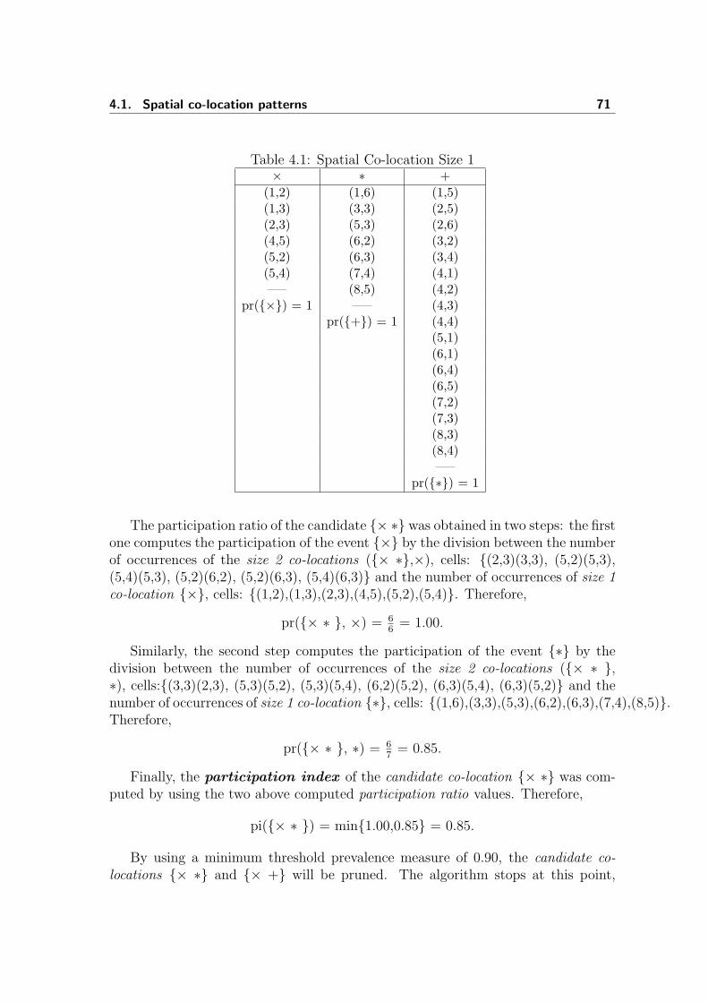
4.1. Spatial co-location patterns 71
Table 4.1: Spatial Co-location Size 1× ∗ +
(1,2) (1,6) (1,5)(1,3) (3,3) (2,5)(2,3) (5,3) (2,6)(4,5) (6,2) (3,2)(5,2) (6,3) (3,4)(5,4) (7,4) (4,1)—– (8,5) (4,2)
pr({×}) = 1 —– (4,3)pr({+}) = 1 (4,4)
(5,1)(6,1)(6,4)(6,5)(7,2)(7,3)(8,3)(8,4)—–
pr({∗}) = 1
The participation ratio of the candidate {× ∗} was obtained in two steps: the firstone computes the participation of the event {×} by the division between the numberof occurrences of the size 2 co-locations ({× ∗},×), cells: {(2,3)(3,3), (5,2)(5,3),(5,4)(5,3), (5,2)(6,2), (5,2)(6,3), (5,4)(6,3)} and the number of occurrences of size 1co-location {×}, cells: {(1,2),(1,3),(2,3),(4,5),(5,2),(5,4)}. Therefore,
pr({× ∗ }, ×) = 66
= 1.00.
Similarly, the second step computes the participation of the event {∗} by thedivision between the number of occurrences of the size 2 co-locations ({× ∗ },∗), cells:{(3,3)(2,3), (5,3)(5,2), (5,3)(5,4), (6,2)(5,2), (6,3)(5,4), (6,3)(5,2)} and thenumber of occurrences of size 1 co-location {∗}, cells: {(1,6),(3,3),(5,3),(6,2),(6,3),(7,4),(8,5)}.Therefore,
pr({× ∗ }, ∗) = 67
= 0.85.
Finally, the participation index of the candidate co-location {× ∗} was com-puted by using the two above computed participation ratio values. Therefore,
pi({× ∗ }) = min{1.00,0.85} = 0.85.
By using a minimum threshold prevalence measure of 0.90, the candidate co-locations {× ∗} and {× +} will be pruned. The algorithm stops at this point,
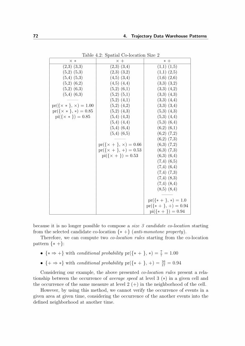
72 4. Trajectory Data Warehouse Patterns
Table 4.2: Spatial Co-location Size 2× ∗ × + ∗ +
(2,3) (3,3) (2,3) (3,4) (1,1) (1,5)(5,2) (5,3) (2,3) (3,2) (1,1) (2,5)(5,4) (5,3) (4,5) (3,4) (1,6) (2,6)(5,2) (6,2) (4,5) (4,4) (3,3) (3,2)(5,2) (6,3) (5,2) (6,1) (3,3) (4,2)(5,4) (6,3) (5,2) (5,1) (3,3) (4,3)
——– (5,2) (4,1) (3,3) (4,4)pr({× ∗ }, ×) = 1.00 (5,2) (4,2) (3,3) (3,4)pr({× ∗ }, ∗) = 0.85 (5,2) (4,3) (5,3) (4,3)pi({× ∗ }) = 0.85 (5,4) (4,3) (5,3) (4,4)
(5,4) (4,4) (5,3) (6,4)(5,4) (6,4) (6,2) (6,1)(5,4) (6,5) (6,2) (7,2)
——– (6,2) (7,3)pr({× + }, ×) = 0.66 (6,3) (7,2)pr({× + }, +) = 0.53 (6,3) (7,3)
pi({× + }) = 0.53 (6,3) (6,4)(7,4) (6,5)(7,4) (6,4)(7,4) (7,3)(7,4) (8,3)(7,4) (8,4)(8,5) (8,4)
——–pr({∗ + }, ∗) = 1.0
pr({∗ + }, +) = 0.94pi({∗ + }) = 0.94
because it is no longer possible to compose a size 3 candidate co-location startingfrom the selected candidate co-location {∗ +} (anti-monotone property).
Therefore, we can compute two co-location rules starting from the co-locationpattern {∗ +}:
• {∗ ⇒ +} with conditional probability pr({∗ + }, ∗) = 77
= 1.00
• {+⇒ ∗} with conditional probability pr({∗ + }, +) = 1617
= 0.94
Considering our example, the above presented co-location rules present a rela-tionship between the occurrence of average speed at level 3 (∗) in a given cell andthe occurrence of the same measure at level 2 (+) in the neighborhood of the cell.
However, by using this method, we cannot verify the occurrence of events in agiven area at given time, considering the occurrence of the another events into thedefined neighborhood at another time.
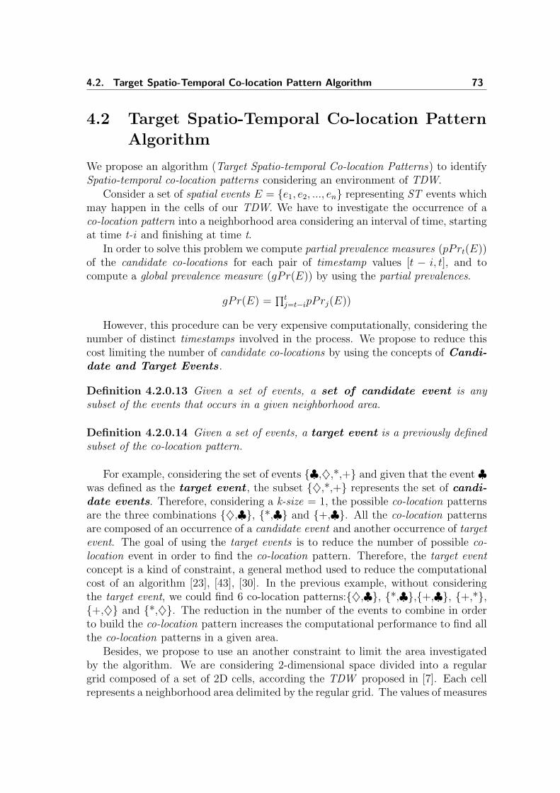
4.2. Target Spatio-Temporal Co-location Pattern Algorithm 73
4.2 Target Spatio-Temporal Co-location Pattern
Algorithm
We propose an algorithm (Target Spatio-temporal Co-location Patterns) to identifySpatio-temporal co-location patterns considering an environment of TDW.
Consider a set of spatial events E = {e1, e2, ..., en} representing ST events whichmay happen in the cells of our TDW. We have to investigate the occurrence of aco-location pattern into a neighborhood area considering an interval of time, startingat time t-i and finishing at time t.
In order to solve this problem we compute partial prevalence measures (pPrt(E))of the candidate co-locations for each pair of timestamp values [t − i, t], and tocompute a global prevalence measure (gPr(E)) by using the partial prevalences.
gPr(E) =∏t
j=t−ipPrj(E))
However, this procedure can be very expensive computationally, considering thenumber of distinct timestamps involved in the process. We propose to reduce thiscost limiting the number of candidate co-locations by using the concepts of Candi-date and Target Events .
Definition 4.2.0.13 Given a set of events, a set of candidate event is anysubset of the events that occurs in a given neighborhood area.
Definition 4.2.0.14 Given a set of events, a target event is a previously definedsubset of the co-location pattern.
For example, considering the set of events {♣,♦,*,+} and given that the event ♣was defined as the target event , the subset {♦,*,+} represents the set of candi-date events. Therefore, considering a k-size = 1, the possible co-location patternsare the three combinations {♦,♣}, {*,♣} and {+,♣}. All the co-location patternsare composed of an occurrence of a candidate event and another occurrence of targetevent. The goal of using the target events is to reduce the number of possible co-location event in order to find the co-location pattern. Therefore, the target eventconcept is a kind of constraint, a general method used to reduce the computationalcost of an algorithm [23], [43], [30]. In the previous example, without consideringthe target event, we could find 6 co-location patterns:{♦,♣}, {*,♣},{+,♣}, {+,*},{+,♦} and {*,♦}. The reduction in the number of the events to combine in orderto build the co-location pattern increases the computational performance to find allthe co-location patterns in a given area.
Besides, we propose to use an another constraint to limit the area investigatedby the algorithm. We are considering 2-dimensional space divided into a regulargrid composed of a set of 2D cells, according the TDW proposed in [7]. Each cellrepresents a neighborhood area delimited by the regular grid. The values of measures
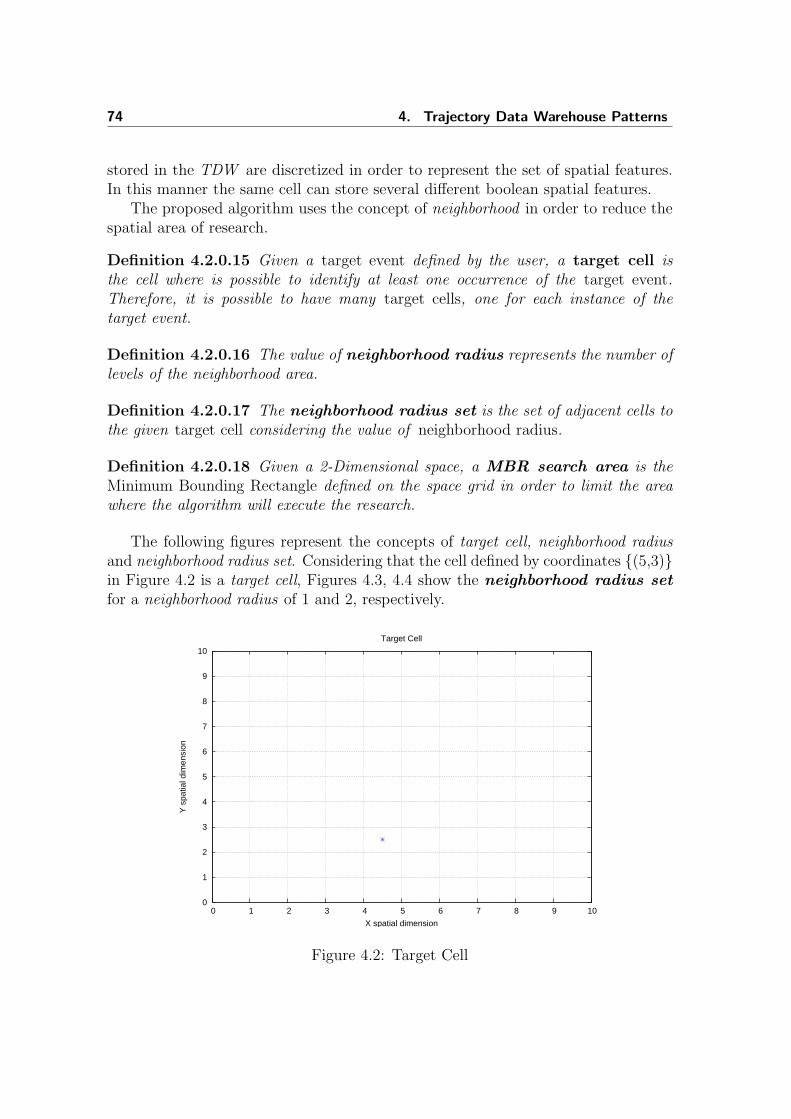
74 4. Trajectory Data Warehouse Patterns
stored in the TDW are discretized in order to represent the set of spatial features.In this manner the same cell can store several different boolean spatial features.
The proposed algorithm uses the concept of neighborhood in order to reduce thespatial area of research.
Definition 4.2.0.15 Given a target event defined by the user, a target cell isthe cell where is possible to identify at least one occurrence of the target event.Therefore, it is possible to have many target cells, one for each instance of thetarget event.
Definition 4.2.0.16 The value of neighborhood radius represents the number oflevels of the neighborhood area.
Definition 4.2.0.17 The neighborhood radius set is the set of adjacent cells tothe given target cell considering the value of neighborhood radius.
Definition 4.2.0.18 Given a 2-Dimensional space, a MBR search area is theMinimum Bounding Rectangle defined on the space grid in order to limit the areawhere the algorithm will execute the research.
The following figures represent the concepts of target cell, neighborhood radiusand neighborhood radius set. Considering that the cell defined by coordinates {(5,3)}in Figure 4.2 is a target cell, Figures 4.3, 4.4 show the neighborhood radius setfor a neighborhood radius of 1 and 2, respectively.
0
1
2
3
4
5
6
7
8
9
10
0 1 2 3 4 5 6 7 8 9 10
Y s
patia
l dim
ensi
on
X spatial dimension
Target Cell
Figure 4.2: Target Cell
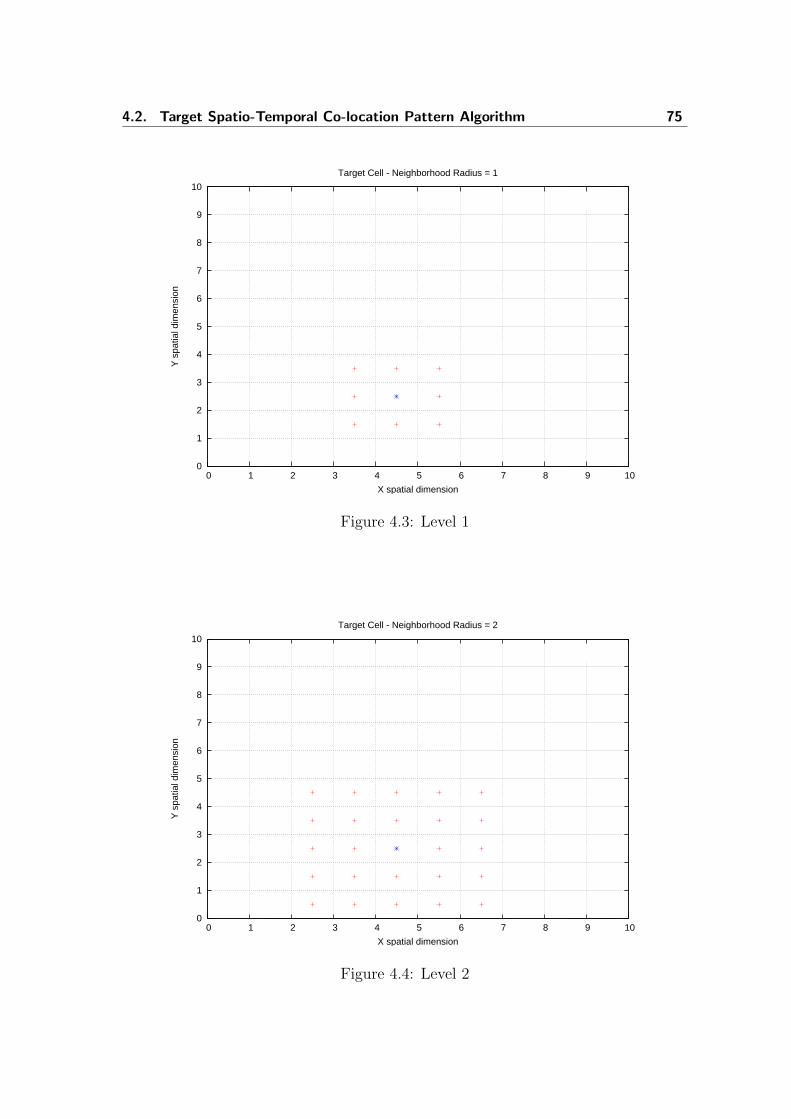
4.2. Target Spatio-Temporal Co-location Pattern Algorithm 75
0
1
2
3
4
5
6
7
8
9
10
0 1 2 3 4 5 6 7 8 9 10
Y s
patia
l dim
ensi
on
X spatial dimension
Target Cell - Neighborhood Radius = 1
Figure 4.3: Level 1
0
1
2
3
4
5
6
7
8
9
10
0 1 2 3 4 5 6 7 8 9 10
Y s
patia
l dim
ensi
on
X spatial dimension
Target Cell - Neighborhood Radius = 2
Figure 4.4: Level 2

76 4. Trajectory Data Warehouse Patterns
After defining and computing the Target Events, the procedure uses the defini-tions proposed in [54]. We have to compute participation ratio and participationindex values for each pair of timestamps. This computation is reduced by using theTarget Events, we just have to compute the participation ration and index values forthe Target Events. The algorithm has two main phases: (i)Definition of the searchspatio-temporal area and (ii) Computation of the space and time prevalence values.
In the first step we delimitate the area where the search of the patterns will beexecuted. Besides, we delimitate the target neighborhood areas. Figure 4.5 presentsa view of fundamental concepts (MBR Search Area, 2 Target Cells and 2 TargetNeighborhood Area) of the algorithm on an area divided according to a regulargrid. The target neighborhood area is a set of disjoint areas obtained from theneighborhood of the cells where happens an occurrence of a target event. TargetEvents are events defined by the user in order to execute the algorithm. For example,when the goal is to find a co-location occurrence composed of traffic jam event anda set of other events, traffic jam is defined as a target event. The computation ofthe prevalence values (space and time) by using the values stored in cells involvedby the target neighborhood area it is performed in the second step.
Figure 4.5: Target Spatio-Temporal Colocation Concepts
Algorithm 3 presents the pseudo-code of the Target Spatio-Temporal Co-locationPattern Algorithm. In the following we discuss the details of each step.

4.2. Target Spatio-Temporal Co-location Pattern Algorithm 77
Algorithm 3 Target Spatio-Temporal Co-location Pattern AlgorithmInput. A relation R where each record represent a specific cell x, y, t and the discretized valuesfor each TDW measure.. User defined Target Events Set. A user defined Neighborhood radius. Timestamp Values. MBR search area. A user specified minimum threshold prevalence measure (min prevalence)Output. Co-location patterns with partition index > min prevalenceMethod
1: Generate search area2: Find the cells (Target Cells) with at least an occurrence of the defined Target Events3: Find the neighborhood area related for each Target Cells4: Generate Candidate Events size 15: for size of co-locations in (1,2,3,..., K - 1) do6: Generate candidate prevalent co-locations by using the previous co-location pattern
stored in the Frequent Pattern Table.7: Compute the space and time prevalence measures for each candidate co-location
pattern and prune by using the (min prevalence) value.8: end for
Step 1 By using the input values, the first step is to generate the search areathat will be used to limit the space area to find co-location patterns. Thecoordinates that limit the research area are stored in the Search Area Table,it is a structure used to search the delimited area for the complete timestampinterval.
Step 2 Once defined and stored the boundaries of the research area, in this stepit is executed the process to select the Target Cells. This process, by usingthe target timestamp and the boundaries of the Search area, searches the cellswhere at least one occurrence of the Target Event happens. These values (cellcoordinates) will be stored in a structure named Target Cells Table.
Step 3 In this step we define the neighborhood area for each record stored in TargetCells Table. To this end, we use the Neighborhood radius value to limit theneighborhood area for each target cell. These values are stored in a structurenamed Target Neighborhood Area Table.
Steps 4-5 In these steps we complete the process of finding Candidate Events size1. The first point is to select (for each timestamp) the candidate events foreach neighborhood area. These candidate events are the source to computethe prevalence measures for each candidate co-location composed by using

78 4. Trajectory Data Warehouse Patterns
the Target Events and the candidate events. The candidate co-location pat-terns size 1 will be selected considering the user-defined prevalence threshold(min prevalence). The candidate co-location patterns size 1 with prevalencevalue above or equal to the min prevalence will be stored in a structure namedFrequent pattern. These values are the data source to the next steps of thealgorithm.
Steps 5-8 A loop to compose the candidate co-location patterns starting from thecandidate co-location size 1. Steps 6 and 7 are complementary, each recordproduced in the Step 6 it is complemented by an execution of the Step 7. Fre-quent Pattern Table is ordered by size of co-location (k) and co-location pat-tern. In Step 6 each value of co-location pattern with co− locationsize = k−1it is combined with the consequent co-location pattern in order to compose acandidate co-location pattern with co − locationsize = k. Then, for eachcandidate co-location pattern size k, the Step 7 computes the space and timeprevalence measures. This computation is executed considering the limited re-search area and the neighborhood area. Considering that the Frequent PatternTable is ordered, the number of items used to compute each execution of theStep 6 decreases after each execution.
In the next Section we present an example of execution of the algorithm. Itconsiders three timestamps and three different TDW values. For simplicity, theexample uses just one TDW measure for cell.
4.3 Execution Trace of Target Spatio-Temporal
Co-location Pattern Algorithm
Figures 4.6,4.7 and 4.8 represent the MBR search area at three different timestamps,they are used to explain our method. We consider an environment composed of aset of events {A, B, C, T} (Candidate Events) and their instances over the spatio-temporal area: A{A.1, A.2, A.3, A.4}, B{B.1, B.2, B.3, B.4, B.5, B.6, B.7} andC{C.1, C.2, C.3, C.4, C.5}.
In this case, the event (T ) is the Target Event . We are interested in finding aco-location pattern composed of different events occurring in the time interval [t−i, t].The distance between events are defined in terms of both time and space. Figures4.6,4.7 and 4.8 present the environment at times (t-2), (t-1) and (t), respectively.They present the area divided into a regular grid. In this example we consider onlyone instance of the event for each cell. The line between two instances representsa neighbor relationship. The cells where the Target Event (T ) happens at timet (Step 11 ) are used to define the neighborhood area (Step 12 ). The bold linesaround the cells with an occurrence of the instance T (Target cell) represent theboundaries of the neighborhood radius set area (AreaI, AreaII and AreaIII ). Besides,

4.3. Execution Trace of Target Spatio-Temporal Co-location Pattern Algorithm 79
figures present three boxes with the computed value of participation ratio for eachcandidate co-location pattern. In this case the goal is to find a co-location patternby using the T event at time t as the Target Event. We are considering a thresholdmeasure of prevalence of 0.55.
For each figure, the space distance component represents the 9 adjacent cellsaround each Target cell. The figures present three Target cells and three neigh-borhood radius set areas, one for each Target cell, considering area composed of 9adjacent cells.
//
OO
C.4
C.5
C.3
A.3GFED@ABC
T76540123'&%$ !"#���������
A.2GFED@ABC A.4GFED@ABC
B.1
T76540123'&%$ !"#�������
A.1GFED@ABC
T76540123'&%$ !"#4444444
B.2 TTTTT
T76540123'&%$ !"#
C.1C.2
B.3
B.4
B.5 T76540123'&%$ !"# B.7T76540123'&%$ !"#T76540123'&%$ !"#B.6
Pr({T,A},A) = 24
= 0.50
Pr({T,B},B) = 57
= 0.71
Pr({T,C},C) = 15
= 0.20
AreaI
AreaII
AreaIII
Figure 4.6: Neighborhood t - 2
In Figure 4.6, the time distance component represents the environment at time(t-2). Considering the event T as the Target Event, it is possible to find threedifferent candidate co-location: {T, A}, {T,B} and {T, C}. In the following thecandidate instances for each area of Figure 4.6:
AreaI {A.1, B.1, B.2, T}
AreaII {A.3, B.5, B.6, B.7, T}
AreaIII {C.1, T}
The computation of Participation ratio for each candidate co-location it is pre-sented in the following:

80 4. Trajectory Data Warehouse Patterns
• Pr({T,A}, A) = 24, 2 out of 4 instances of A (A.1,A.3) is contributing to the
co-location {T, A}
• Pr({T,B}, B) = 57, 5 out of 7 instances of B (B.1,B.2,B.5,B.6,B.7) is con-
tributing to the co-location {T, B}
• Pr({T,C}, C) = 15, 1 out of 5 instances of C (C.1) is contributing to the
co-location {T, C}
//
OO
C.4
C.5
A.4GFED@ABC
T76540123'&%$ !"#
B.1
9999
9999
B.2 T76540123'&%$ !"#
C.2
C.1
T76540123'&%$ !"#A.1GFED@ABCT76540123'&%$ !"#
tttttt
A.2GFED@ABCT76540123'&%$ !"#TTTTT C.3
B.5
T76540123'&%$ !"#�������
B.4
B.3
A.3GFED@ABCT76540123'&%$ !"#B.7 T76540123'&%$ !"#B.6
T76540123'&%$ !"# Pr({T,A},A) = 34
= 0.75
Pr({T,B},B) = 47
= 0.57
Pr({T,C},C) = 25
= 0.40
AreaI
AreaII
AreaIII
Figure 4.7: Neighborhood t - 1
In Figure 4.7, the time distance component represents the environment at time(t-1). Considering the event T as the Target Event, it is possible to find threedifferent candidate co-location: {T,A}, {T, B} and {T, C}. In the following thecandidate instances for each area of Figure 4.7:
AreaI {A.1, A.2, B.1, T}
AreaII {A.3, B.5, B.6, B.7, T}
AreaIII {C.1, C.2, T}
The computation of Participation ratio for each candidate co-location it is pre-sented in the following:
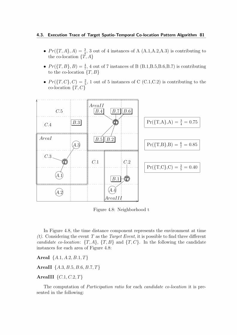
4.3. Execution Trace of Target Spatio-Temporal Co-location Pattern Algorithm 81
• Pr({T, A}, A) = 34, 3 out of 4 instances of A (A.1,A.2,A.3) is contributing to
the co-location {T, A}
• Pr({T, B}, B) = 47, 4 out of 7 instances of B (B.1,B.5,B.6,B.7) is contributing
to the co-location {T,B}
• Pr({T, C}, C) = 25, 1 out of 5 instances of C (C.1,C.2) is contributing to the
co-location {T,C}
//
OO
A.1GFED@ABCT76540123'&%$ !"#�����
A.2GFED@ABC A.4GFED@ABCT76540123'&%$ !"#
xxxxxx
A.3GFED@ABC
T76540123'&%$ !"#
T76540123'&%$ !"#
C.2
B.1 T76540123'&%$ !"#
C.1C.3
T76540123'&%$ !"#TTTTT
C.4
C.5
B.3
B.2
T76540123'&%$ !"#�������
B.5
T76540123'&%$ !"#���������
B.4
T76540123'&%$ !"#JJJJJJ B.7
T76540123'&%$ !"#B.6
T76540123'&%$ !"# ����
�
Pr({T,A},A) = 34
= 0.75
Pr({T,B},B) = 67
= 0.85
Pr({T,C},C) = 25
= 0.40
AreaI
AreaII
AreaIII
Figure 4.8: Neighborhood t
In Figure 4.8, the time distance component represents the environment at time(t). Considering the event T as the Target Event, it is possible to find three differentcandidate co-location: {T,A}, {T,B} and {T, C}. In the following the candidateinstances for each area of Figure 4.8:
AreaI {A.1, A.2, B.1, T}
AreaII {A.3, B.5, B.6, B.7, T}
AreaIII {C.1, C.2, T}
The computation of Participation ratio for each candidate co-location it is pre-sented in the following:

82 4. Trajectory Data Warehouse Patterns
• Pr({T,A}, A) = 34, 3 out of 4 instances of A (A.1,A.3,A.4) is contributing to
the co-location {T,A}
• Pr({T,B}, B) = 67, 6 out of 7 instances of B (B.1,B.2,B.4,B.5,B.6,B.7) is
contributing to the co-location {T, B}
• Pr({T,C}, C) = 25, 2 out of 5 instances of C (C.2,C.3) is contributing to the
co-location {T, C}
At this point, the algorithm has three different values of participation ratio foreach candidate co-location. Each of them computed for a different timestamp, in thisexample we considered three timestamps: {t−2, t−1, t}. The next step is to computethe value of participation index for each candidate co-location ({T,A}, {T, B}, {T, C}).According to the proposed algorithm it can be computed by using the minimum valueamong of them (see Definition 3.4.0.8). In the following we present the computationof the participation index for each candidate co-location pattern:
• Pi({T,A}) = min(Pr(t−2){T, A}, P r(t−1){T, A}, P r(t){T,A}) = 24
• Pi({T,B}) = min(Pr(t−2){T,B}, P r(t−1){T,B}, P r(t){T, B}) = 47
• Pi({T,C}) = min(Pr(t−2){T, B}, P r(t−1){T, B}, P r(t){T,B}) = 15
The following step is to compute the time component of the participation index(prevalence time) for each candidate co-location pattern. It is computed by thedivision between the number of timestamps where the candidate co-location patternoccurs and the total number of timestamps. This value represents a fundamentalknowledge about the pattern, it is possible to understand the weight of the patternalong the time interval.
• Pt{T, A} = 33
= 1.0
• Pt{T, B} = 33
= 1.0
• Pt{T, C} = 33
= 1.0
Finally, by using the values of participation index and prevalence time it is possi-ble to compute the Global Participation Index (GPI ) for each candidate co-locationpattern.
• GPI{T, A} = Pi({T, A}) × Pt{T, A} = 24× 3
3= 2
4= 0.50
• GPI{T, B} = Pi({T, B}) × Pt{T, B} = 47× 3
3= 4
7= 0.57
• GPI{T, C} = Pi({T, C}) × Pt{T,C} = × 15
33
= 15
= 0.20

4.3. Execution Trace of Target Spatio-Temporal Co-location Pattern Algorithm 83
After computing the Global Participation Index for each candidate co-location,the next step is pruning. It is done comparing the threshold value of prevalencewith the global participation index computed for each candidate co-location. In thisexample the threshold value of presence is 0.55. Therefore, the only candidate co-location selected is {T, B}, its GPI is 0.57.
That pattern means that an B event at timestamp t - 2 and t - 1 has a relation-ship (into a neighborhood) with a T pattern starting at time t with a prevalencelevel of 0.57. However, we can not affirm that all the occurrences of pattern T attimestamp t are originated at timestamps t-2 or t - 1.
In this example we have defined a Target Event composed by only one TDWmeasure. We have done it in order to facilite the explanation of the method. How-ever, the Target Event can be composed of several TDW measures.
Therefore, by using this model it is possible, for example, to investigate thebehavior of a Traffic Jam Event along the time considering a given area of research.A Traffic Jam event (in this case a Target Event) may be defined by using, forexample, two discretized TDW measures: level of speed (See Equation 2.7) anddensity of presence (See Equation 2.6). In this manner the algorithm may revealthe evolution of a Traffic Jam occurrence by using the TDW measures.
Table 4.3: Prevalence Time x Participation IndexParticipation Ratio - Cases
TimeStamp A B C D E F Gt− 1 0.90 0.90 0.60 0.80 0.20 0.60 0.90t− 2 0.50 0.80 0.90 0.90 0.80 0.80t− 3 0.70 0.50 0.70 0.80 0.80t− 4 0.40 0.90 0.90 0.80t− 5 0.90 0.80 0.70t− 6 0.90 0.80t− 7 0.90
Participation Index (Pi) 0.90 0.50 0.60 0.40 0.20 0.60 0.70Prevalence Time (Pt) 0.14 0.29 0.43 0.57 0.71 0.86 1.00
Global Participation Index (Pi× Pt) 0.13 0.14 0.25 0.22 0.14 0.51 0.70
Prevalence time is a fundamental concept of the proposed algorithm. This valuemeasures the occurrence of the pattern along the time dimension. It is the quo-tient between the number of timestamps that the pattern occurs and the numberof timestamps. Table 4.3 presents an example to explain the importance of theprevalence time. The example presents values of participation ratio for 7 hypotheticco-location patterns (A,B,C,D,E,F and G) by using 7 different timestamps. Givena prevalence measure of 0.30, and considering just the Participation Index measure,cases A, B,C,D,F and G are considered valid patterns. However, when Time preva-lence is computed the situation is totally different, in our example, in this case, onlycases F and G are considered valid. The row Global Participation Index presents
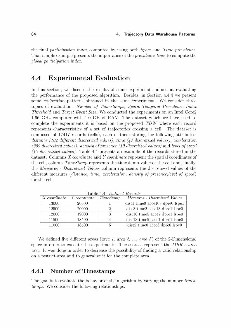
84 4. Trajectory Data Warehouse Patterns
the final participation index computed by using both Space and Time prevalence.That simple example presents the importance of the prevalence time to compute theglobal participation index.
4.4 Experimental Evaluation
In this section, we discuss the results of some experiments, aimed at evaluatingthe performance of the proposed algorithm. Besides, in Section 4.4.4 we presentsome co-location patterns obtained in the same experiment. We consider threetopics of evaluation: Number of Timestamps, Spatio-Temporal Prevalence IndexThreshold and Target Event Size. We conducted the experiments on an Intel Core21.66 GHz computer with 1.0 GB of RAM. The dataset which we have used tocomplete the experiments it is based on the proposed TDW where each recordrepresents characteristics of a set of trajectories crossing a cell. The dataset iscomposed of 17417 records (cells), each of them storing the following attributes:distance (102 different discretized values), time (44 discretized values), acceleration(259 discretized values), density of presence (19 discretized values) and level of speed(13 discretized values). Table 4.4 presents an example of the records stored in thedataset. Columns X coordinate and Y coordinate represent the spatial coordinates ofthe cell, column TimeStamp represents the timestamp value of the cell and, finally,the Measures - Discretized Values column represents the discretized values of thedifferent measures (distance, time, acceleration, density of presence,level of speed)for the cell.
Table 4.4: Dataset RecordsX coordinate Y coordinate TimeStamp Measures - Discretized Values
13000 20500 1 dist1 time0 acce108 dpre0 lspe112500 20000 2 dist8 time2 acce13 dpre1 lspe012000 19000 3 dist16 time5 acce7 dpre1 lspe011500 18500 4 dist13 time5 acce7 dpre1 lspe011000 18500 5 dist2 time0 acce3 dpre0 lspe0
We defined five different areas (area 1, area 2, ..., area 5 ) of the 2-Dimensionalspace in order to execute the experiments. These areas represent the MBR searcharea. It was done in order to decrease the possibility of finding a valid relationshipon a restrict area and to generalize it for the complete area.
4.4.1 Number of Timestamps
The goal is to evaluate the behavior of the algorithm by varying the number times-tamps. We consider the following relationships:
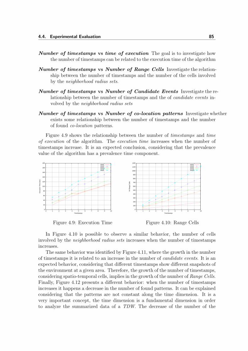
4.4. Experimental Evaluation 85
Number of timestamps vs time of execution The goal is to investigate howthe number of timestamps can be related to the execution time of the algorithm
Number of timestamps vs Number of Range Cells Investigate the relation-ship between the number of timestamps and the number of the cells involvedby the neighborhood radius sets.
Number of timestamps vs Number of Candidate Events Investigate the re-lationship between the number of timestamps and the of candidate events in-volved by the neighborhood radius sets
Number of timestamps vs Number of co-location patterns Investigate whetherexists some relationship between the number of timestamps and the numberof found co-location patterns.
Figure 4.9 shows the relationship between the number of timestamps and timeof execution of the algorithm. The execution time increases when the number oftimestamps increase. It is an expected conclusion, considering that the prevalencevalue of the algorithm has a prevalence time component.
0
20
40
60
80
100
120
140
160
180
200
0 1 2 3 4 5 6 7 8 9 10
Exe
cutio
n T
ime
(sec
)
TimeStamps
area1area2area3area4area5
Figure 4.9: Execution Time
0
100
200
300
400
500
600
700
800
900
1000
1100
1200
0 1 2 3 4 5 6 7 8 9 10
Nr
Ran
ge C
ells
TimeStamps
area1area2area3area4area5
Figure 4.10: Range Cells
In Figure 4.10 is possible to observe a similar behavior, the number of cellsinvolved by the neighborhood radius sets increases when the number of timestampsincreases.
The same behavior was identified by Figure 4.11, where the growth in the numberof timestamps it is related to an increase in the number of candidate events. It is anexpected behavior, considering that different timestamps show different snapshots ofthe environment at a given area. Therefore, the growth of the number of timestamps,considering spatio-temporal cells, implies in the growth of the number of Range Cells.Finally, Figure 4.12 presents a different behavior: when the number of timestampsincreases it happens a decrease in the number of found patterns. It can be explainedconsidering that the patterns are not constant along the time dimension. It is avery important concept, the time dimension is a fundamental dimension in orderto analyze the summarized data of a TDW. The decrease of the number of the

86 4. Trajectory Data Warehouse Patterns
0
10
20
30
40
50
60
70
80
90
100
110
120
130
140
150
0 1 2 3 4 5 6 7 8 9 10
Nr
Can
dida
te E
vent
s
TimeStamps
area1area2area3area4area5
Figure 4.11: Candidate Events
0
1
2
3
4
5
6
7
8
9
10
11
12
13
14
15
0 1 2 3 4 5 6 7 8 9 10
Nr
Pat
tern
s
TimeStamps
area1area2area3area4area5
Figure 4.12: Patterns
patterns along the time dimension it confirms the evolution of the environment andjustifies the temporal component of the prevalence index. A valid pattern at a giventimestamp t may be invalid at a timestamp t + i. Therefore, an increment in thenumber of timestamps may result in the decrease of the probability of finding apattern. Another interesting conclusion is that the execution time of the algorithmdoes not have relationship with the number of patterns found by the algorithm.
4.4.2 Spatio-Temporal Prevalence Index Threshold
In this case the goal is to investigate the relationship among the value of Spatio-Temporal Prevalence Index Threshold and the evolution of the value of time ex-ecution and the number of patterns. An evident conclusion is that the value ofSpatio-Temporal Prevalence Index Threshold does not have any relationship withRange Cells and Candidate Events. Therefore, we did not investigate the relation-ship among Spatio-Temporal Prevalence Index Threshold and those items.
0
5
10
15
20
25
0 0.2 0.4 0.6 0.8 1
Nr
Pat
tern
s
Prevalence Index
area1area2area3area4area5
Figure 4.13: Prevalence vs Pattern
0
10
20
30
40
50
60
70
80
0 0.2 0.4 0.6 0.8 1
Exe
cutio
n T
ime
(sec
)
Prevalence Index
area1area2area3area4area5
Figure 4.14: Prevalence vs Time
Figures 4.13 and 4.14 allow to verify that low values of spatio-temporal preva-lence measure are related to an increase in the number of patterns found by thealgorithm. Another effect of the low values of prevalence measure it is an increase
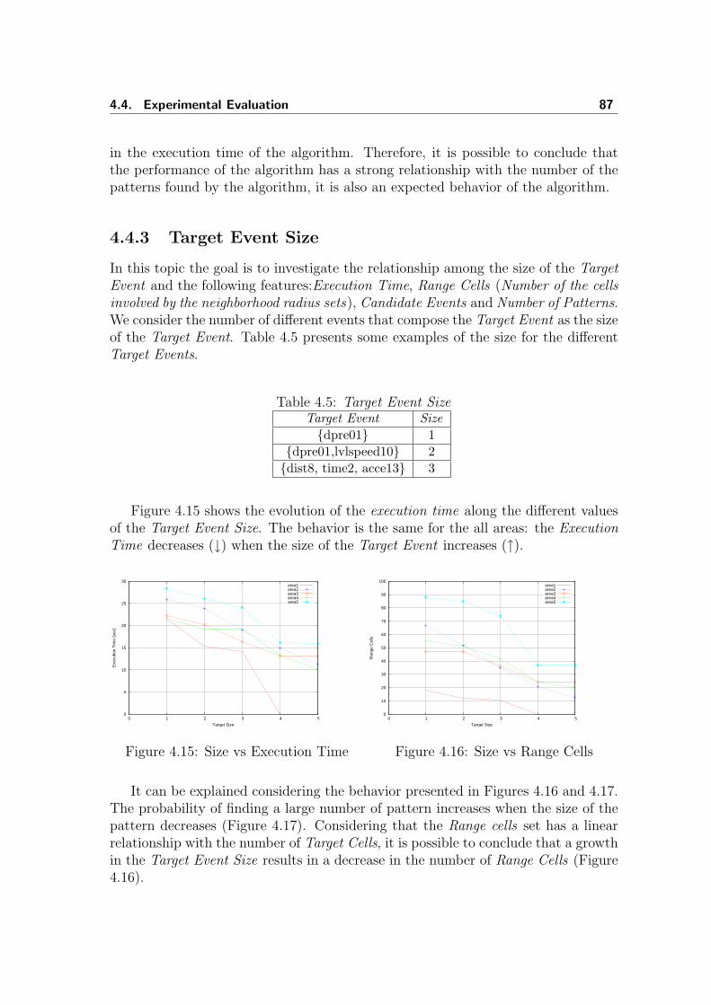
4.4. Experimental Evaluation 87
in the execution time of the algorithm. Therefore, it is possible to conclude thatthe performance of the algorithm has a strong relationship with the number of thepatterns found by the algorithm, it is also an expected behavior of the algorithm.
4.4.3 Target Event Size
In this topic the goal is to investigate the relationship among the size of the TargetEvent and the following features:Execution Time, Range Cells (Number of the cellsinvolved by the neighborhood radius sets), Candidate Events and Number of Patterns.We consider the number of different events that compose the Target Event as the sizeof the Target Event. Table 4.5 presents some examples of the size for the differentTarget Events.
Table 4.5: Target Event SizeTarget Event Size{dpre01} 1
{dpre01,lvlspeed10} 2{dist8, time2, acce13} 3
Figure 4.15 shows the evolution of the execution time along the different valuesof the Target Event Size. The behavior is the same for the all areas: the ExecutionTime decreases (↓) when the size of the Target Event increases (↑).
0
5
10
15
20
25
30
0 1 2 3 4 5
Exe
cutio
n T
ime
(sec
)
Target Size
area1area2area3area4area5
Figure 4.15: Size vs Execution Time
0
10
20
30
40
50
60
70
80
90
100
0 1 2 3 4 5
Ran
ge C
ells
Target Size
area1area2area3area4area5
Figure 4.16: Size vs Range Cells
It can be explained considering the behavior presented in Figures 4.16 and 4.17.The probability of finding a large number of pattern increases when the size of thepattern decreases (Figure 4.17). Considering that the Range cells set has a linearrelationship with the number of Target Cells, it is possible to conclude that a growthin the Target Event Size results in a decrease in the number of Range Cells (Figure4.16).

88 4. Trajectory Data Warehouse Patterns
0
1
2
3
4
5
6
7
8
9
10
11
12
13
14
15
0 1 2 3 4 5
Nr
Pat
tern
s
Target Size
area1area2area3area4area5
Figure 4.17: Size vs Patterns
50
60
70
80
90
100
0 1 2 3 4 5
Nr
Can
dida
te E
vent
s
Target Size
area1area2area3area4area5
Figure 4.18: Size vs Candidate
Another interesting behavior it is presented in Figure 4.18. The number ofCandidate Events remains stable along the evolution of the size of the Target Event.It is an expected behavior considering that we search the same area (MBR Searcharea) for the different size values of the Target Event.
4.4.4 Co-location Patterns
This section presents some co-location patterns obtained by using the proposed al-gorithm. We have used the same dataset described in Section 4.4. The goal is toinvestigate whether is possible to find some co-location patterns considering twodifferent movement phenomenon: Traffic Jam and Free Traffic. We have used aneighborhood radius of 1 and a timestamp range composed of three different times-tamps. Table 4.6 presents some obtained patterns.
Table 4.6: Co-location PatternsCandidate Events Target Event GPI{dist0 dpre0} {Free} 0.83{dist12 dpre0} {Free} 0.60{dist19 dpre0} {Free} 0.66{time0 dpre0} {Free} 0.77{time1 dpre0} {Free} 0.60{075TJ lspe0} {TJ} 1.00{time11 dpre16} {TJ} 0.66{time12 dpre16} {TJ} 0.66{dist56 dpre16} {TJ} 0.66{dpre5 acce3 lspe0} {TJ} 0.66{time7 acce3 lspe0} {TJ} 0.50
It is evident that the co-location patterns can suffer changes regarding the area ofsearch. Patterns may be modified considering different values of neighborhood radiusand timestamp range. However, at this point we only are interested in investigate
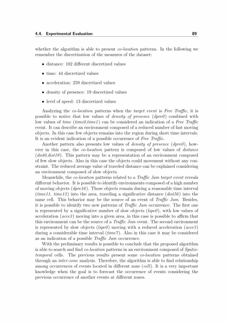
4.4. Experimental Evaluation 89
whether the algorithm is able to present co-location patterns. In the following weremember the discretization of the measures of the dataset:
• distance: 102 different discretized values
• time: 44 discretized values
• acceleration: 259 discretized values
• density of presence: 19 discretized values
• level of speed: 13 discretized values
Analyzing the co-location patterns when the target event is Free Traffic, it ispossible to notice that low values of density of presence (dpre0 ) combined withlow values of time (time0,time1 ) can be considered an indication of a Free Trafficevent. It can describe an environment composed of a reduced number of fast movingobjects. In this case few objects remains into the region during short time intervals.It is an evident indication of a possible occurrence of Free Traffic.
Another pattern also presents low values of density of presence (dpre0 ), how-ever in this case, the co-location pattern is composed of low values of distance(dist0,dist19 ). This pattern may be a representation of an environment composedof few slow objects. Also in this case the objects could movement without any con-straint. The reduced average value of traveled distance can be explained consideringan environment composed of slow objects.
Meanwhile, the co-location patterns related to a Traffic Jam target event revealsdifferent behavior. It is possible to identify environments composed of a high numberof moving objects (dpre16 ). Those objects remain during a reasonable time interval(time11, time12 ) into the area, traveling a significative distance (dist56 ) into thesame cell. This behavior may be the source of an event of Traffic Jam. Besides,it is possible to identify two new patterns of Traffic Jam occurrence. The first oneis represented by a significative number of slow objects (lspe0 ), with low values ofacceleration (acce3 ) moving into a given area, in this case is possible to affirm thatthis environment can be the source of a Traffic Jam event. The second environmentis represented by slow objects (lspe0 ) moving with a reduced acceleration (acce3 )during a considerable time interval (time7 ). Also in this case it may be consideredas an indication of a possible Traffic Jam occurrence.
With the preliminary results is possible to conclude that the proposed algorithmis able to search and find co-location patterns in an environment composed of Spatio-temporal cells. The previous results present some co-location patterns obtainedthrough an inter-zone analysis. Therefore, the algorithm is able to find relationshipamong occurrences of events located in different zone (cell). It is a very importantknowledge when the goal is to forecast the occurrence of events considering theprevious occurrence of another events at different zones.

90 4. Trajectory Data Warehouse Patterns
Conclusions
The recent development of mobility technology (mobile computation, celular phone,remote sensors etc) allows the monitoring of the behavior of moving objects. Themovement of an object can be described by using its trajectory. The analysis ofa trajectory database allows to reveal hidden knowledge about some phenomenaof movement. The knowledge discovery area has been deeply developed in the lastyears. Techniques, concepts and methods to store and manage data are fundamentalto allow the analysis of the large data volumes. Therefore, database and datawarehouse technologies are the base to execute a process of knowledge discovery.Besides, the data mining technology is another indispensable tool to implement acomplete process to reveal hidden knowledge from data volumes. In the recent years,some researches in the usage of the data mining techniques applied to trajectorydatabases were produced. Those researches assume that the trajectory databasestores the memory of the movement of the object. Each record of the databaserepresent a spatio-temporal position of the moving object.
However, in this thesis we have analyzed the problem to mine and aggregate mea-sures concerning trajectories of moving objects. We have assumed that the databasedoes not maintain the memory of the trajectories for each moving object. We haveproposed a multi-dimensional data model to store aggregate measures computed overtrajectory data. This allowed us to define a Trajectory Data Warehouse (TDW ) thatis loaded by managing and transforming a data stream of spatio-temporal observa-tions of moving objects, arriving in a irregular and unbounded way. We have useda traditional star schema composed of two spatial dimensions and one temporal di-mension. The base cuboid is composed of spatio-temporal cells, consisting of regionsand time intervals. We have associated concepts hierarchies with spatial and tempo-ral attributes. The spatial cube was built as the lattice of cuboids, where the lowestone references all the dimensions at the primitive abstraction level. The others areobtained by summarizing on different subsets of the dimensions, and at different ab-straction levels along the concept hierarchy. The Trajectory Data Warehouse allowsto find aggregate measures regarding the trajectories involved in a given area andtime interval. Those measure represents properties about the trajectories. We haveintroduced an aggregated function called Presence. This function represents thecount of the distinct trajectories crossing a given cell, it is a holistic function. Thistype of function, when applied to a data stream source are often computed in anapproximated way. We introduced two approximate functions in order to computethe measure Presence: Distributive and Algebraic. These alternative functions onlyneed a few/constant memory size for maintaining the information.
We have developed a prototype in order to validate the proposed TDW and the

92 Conclusions
associated measures. The prototype implements all the concepts and features ofthe Trajectory Data Warehouse. We have conducted some experiments in order tomeasure the accuracy of the presence measure. Besides, we also have investigated thetime taken to load the cube of the TDW, it is a fundamental characteristic in orderto implement the TDW schema by using commercial data warehouse products. Allthe obtained results allow to affirm that the proposed Trajectory Data Warehouseoffers an environment to receive, process and store trajectory data by using themultidimensional concept. Besides, considering that the TDW works on a datastream environment, it is an adequate solution to the data stream features. Futureworks may investigate the loading phase of the TDW. It is an opened problem, wehave limited the loading phase considering a linear interpolation. However, it ispossible to find topological constraints where the proposed interpolation does notsolve the problem. Besides, the improvement of the current dimensions is a point tobe investigate in the future works. The idea is to investigate the implementation ofthe complete spatial dimensions defined in [60]. It could be useful to answer queriesinvolving a geometric operation such as a spatial union, a spatial merge or a spatialintersection. Another investigation is the possibility of the development of a querylanguage using OLAP operators.
We have done an investigation to verify whether the proposed TDW allows, byanalyzing the stored measures, to reveal the occurrence of events in a given area.Actually, we have considered a Traffic Jam (TJ ) occurrence. We have proposed toinvestigate a TJ occurrence by using two measures to represent the context of a givencell: level of speed and density of presence. These measures can be computed onthe basis of those stored in the TDW along with the statically available measures.The results obtained in the experiments allow to consider the measures densityof presence and level of speed enough to investigate the occurrence of TJ events.We have obtained a high level of accuracy to find TJ occurrences considering thecells whose level of traffic jam is into the following intervals: [0.00%, 25.00%] or[75.00%, 100.00%]. Therefore, a possible future research may be to investigate newmethods/algorithms to improve the accuracy of results analyzing cells whose levelof TJ is into the interval (25.00%, 75.00%).
We proposed an algorithm to mine co-location patterns of events by using theTrajectory Data Warehouse model as data source. We considered that an event in anenvironment of trajectories of moving objects can be represented by a combinationof the TDW measures. The algorithm is based on the proposals presented in [12],[11] and [31]. The proposed Target Event Co-location Pattern algorithm was definedto work by using the data stored in a Trajectory Data Warehouse. The goal is tofind, in a delimited area defined by the user, occurrences of co-location patternsamong events of movement of objects. In order to reduce the computational costinvolved in this process the algorithm finds the complement of a co-location patternby using the concepts of target and candidate event. We used the concept of MBRsearch area in order to reduce the area of search. It was done in order to reduce thecomputational cost to execute the algorithm. The algorithm allows to forecast the

Conclusions 93
occurrence of events of movement in a given area investigating the occurrences ofanother related events that occur in the neighborhood area.
We done several experiments in order to investigate the relationship among sev-eral features: Number of Timestamps, Spatio-Temporal Prevalence Index Threshold,Target Event Size, Execution Time, Number of Range Cells, Number of CandidateEvents and Number of co-location patterns. The results confirm the importance ofthe temporal component in the Spatio-temporal prevalence measure. The temporalcomponent allows to investigate the occurrence of a co-location pattern along thetime dimension. It is possible to define a time-window to investigate the pattern,and find patterns that are prevalent at a given area and also prevalent along thedefine time-window. Besides, it reduces the computational cost to execute the al-gorithm reducing the number of candidate events to compose the final co-locationpattern.
The mined patterns are useful to improve the capability of analysis of a TDWenvironment. The patterns allow to understand the relationship among the eventsalong the time at different areas. These patterns may reveal, for example, differentrelationships among antecedent and consequent (target) events at different areas.The antecedent event for a same target event may be different at different areas ordifferent timestamps.
We implemented the algorithm by using the measures defined in the our proposedTDW. However, another different measures may be used in the algorithm, one ofthem it is correlation. Correlation indicates the strength and direction of a linearrelationship between two variables. An example of the usage of the correlationmeasure may be to identify an occurrence of a traffic jam event when the valuesof density of presence increases (↑), and the values of level of speed decreases (↓).The correlation measure may be useful to find more detailed relationship among themeasures of the TDW.
Another research point to be investigated it is the time constraint. We are focuson the definition of the time interval between successive events occurrences. Thisconstraint allows to improve the capability of anticipating the occurrence of a givenpattern. A same complete pattern (antecedent and target events) may have differentbehavior considering the time gap between them. For example: the pattern 〈A, BC〉at a given area may have time gap between the events of 10 minutes. Meanwhile,at a different area the same pattern may have a time gap of 70 minutes. In thiscase, the same pattern can reveal different events. Therefore, the time constraint isa very important point to be exploited in the future research.

94 Conclusions

Bibliography
[1] S. Chamberlain A. Sistla, O. Wolfson and S. Dao. Modeling and queryingmoving objects. In ICDE’97, pages 422–432, 1997.
[2] R. Agrawal, T. Imielinski, and A. N. Swami. Mining association rules betweensets of items in large databases. Proceedings of the ACM International Confer-ence on Management of Data, pages 207–216, 1993.
[3] R. Agrawal and R. Srikant. Mining sequential patterns. In Philip S. Yu andArbee S. P. Chen, editors, Eleventh International Conference on Data Engi-neering, pages 3–14, Taipei, Taiwan, 1995. IEEE Computer Society Press.
[4] Y. Bdard, S. Rivest, and M. J. Proulx. Spatial On-Line Analytical Processing(SOLAP): Concepts, Architectures and Solutions from a Geomatics EngineeringPerspective., chapter Data Warehouses and OLAP: Concepts, Architectures andSolutions. Idea Group Publishing, 2006.
[5] F. Braz. Knowledge discovery on trajectory data warehouses: Possible usageof the data mining techniques. In SBSI 2008: Proceedings of the 4th BrazilianSymposium on Informatics, Rio de Janeiro,Rio de Janeiro,Brazil, 2008. SBCBrazilian Computer Society.
[6] F. Braz and S. Orlando. Trajectory data warehouses: Proposal of design andapplication to exploit data. In GEOINFO 2007: Proceedings of the 9th BrazilianSymposium on Geoinformatics, Campos do Jordao,Sao Paulo,Brazil, 2007. SBCBrazilian Computer Society.
[7] F. Braz, S. Orlando, R. Orsini, A. Raffaet, A. Roncato, and C. Silvestri. Ap-proximate aggregations in trajectory data warehouse. In Proc. of ICDE Work-shop STDM, pages 536–545, 2007.
[8] T. Brinkhoff. Generating network-based moving objects. In SSDBM ’00:Proceedings of the 12th international Conference on Scientific and StatisticalDatabase Management, page 253, Washington,DC,USA, 2000. IEEE ComputerSociety.
[9] H. Cao, N. Mamoulis, and D. W. Cheung. Mining frequent spatio-temporalsequential patterns. In ICDM ’05: Proceedings of the Fifth IEEE InternationalConference on Data Mining, pages 82–89, Washington, DC, USA, 2005. IEEEComputer Society.

96 Bibliography
[10] H. Cao, N. Mamoulis, and D. W. Cheung. Discovery of collocation episodesin spatiotemporal data. In ICDM ’06: Proceedings of the Sixth InternationalConference on Data Mining, pages 823–827, Washington, DC, USA, 2006. IEEEComputer Society.
[11] M. Celik, J. M. Kang, and S. Shekhar. Zonal co-location pattern discoverywith dynamic parameters. In ICDM ’07: Proceedings of the 2007 SeventhIEEE International Conference on Data Mining, pages 433–438, Washington,DC, USA, 2007. IEEE Computer Society.
[12] M. Celik, S. Shekhar, J. P. Rogers, and J. A. Shine. Mixed-drove spatio-temporal co-occurence pattern mining. In IEEE Transactions on Knowledgeand Data Engineering, Washington, DC, USA, 2008. IEEE Computer Society.
[13] P. Kalnis D. Papadias, Y. Tao and J. Zhang. Indexing spatio-temporal datawarehouses. In ICDE’02, pages 166–175, 2002.
[14] M. L. Damiani and Stefano Spaccapietra. Spatial data warehouse modelling.In Processing and Managing Complex Data for Decision Support. Idea GroupPublishing, 2006.
[15] J. Eder and C. Koncilia. Data Warehousing and Knowledge Discovery, vol-ume Volume 2114/2001, chapter Changes of Dimension Data in Temporal DataWarehouses, pages 284–293. Springer Berlin / Heidelberg, 2001.
[16] U. Fayyad, G. Piatetsky-Shapiro, and P. Smyth. From data mining to knowl-edge discovery: an overview. In Advances in knowledge discovery and datamining, pages 1–34, Menlo Park, CA, USA, 1996. American Association forArtificial Intelligence.
[17] U. Fayyad, G. Piatetsky-Shapiro, and P. Smyth. The kdd process for extractinguseful knowledge from volumes of data. Commun. ACM, 39(11):27–34, 1996.
[18] U. Fayyad, G. Piatetsky-shapiro, and P. Smyth. Knowledge discovery and datamining: Towards a unifying framework. In Proc. 2nd Int. Conf. on KnowledgeDiscovery and Data Mining, pages 82–88. AAAI Press, 1996.
[19] U. Fayyad, G. Piatetsky-Shapiro, and P. Smyth. Modeling multidimensionalspatio-temporal data warehouses in a context of evolving specifications. InGeospatial Theory, Processing and Applications, volume XXXIV, 2002.
[20] U. Fayyad, G. Piatetsky-Shapiro, P. Smyth, and R. Uthurusamy, editors. Ad-vances in knowledge discovery and data mining. American Association for Ar-tificial Intelligence, Menlo Park, CA, USA, 1996.
[21] P. Flajolet and G. Martin. ”probabilistic counting algorithms for data baseapplications”. Journal of Computer and System Sciences, 31(2):182–209, 1985.
Bibliography 97
[22] V. Ganti, J. Gehrke, and R. Ramakrishnan. Mining very large databases.Computer, 32(8):38–45, 1999.
[23] M. N. Garofalakis, R. Rastogi, and K. Shim. Spirit: Sequential pattern min-ing with regular expression constraints. In M. P. Atkinson, M. E. Orlowska,P. Valduriez, S. B. Zdonik, and M. L. Brodie, editors, VLDB’99, Proceedingsof 25th International Conference on Very Large Data Bases, September 7-10,1999, Edinburgh, Scotland, UK, pages 223–234. Morgan Kaufmann, 1999.
[24] F. Giannotti, M. Nanni, F. Pinelli, and D. Pedreschi. Trajectory pattern mining.In KDD ’07: Proceedings of the 13th ACM SIGKDD international conferenceon Knowledge discovery and data mining, pages 330–339, New York, NY, USA,2007. ACM.
[25] G. Gidfalvi. Mining long, sharable patterns in trajectories of moving objects.GeoInformatica, 2007.
[26] J. Gray, S. Chaudhuri, A. Bosworth, A. Layman, D. Reichart, M. Venkatrao,F. Pellow, and H. Pirahesh. Data cube: A relational aggregation operatorgeneralizing group-by, cross-tab and sub-totals. Data Mining and KnowledgeDiscovery, 1:29–54, 1997.
[27] J. Gudmundsson and M. van Kreveld. Computing longest duration flocks intrajectory data. In GIS ’06: Proceedings of the 14th annual ACM internationalsymposium on Advances in geographic information systems, pages 35–42, NewYork, NY, USA, 2006. ACM.
[28] J. Gudmundsson, M. van Kreveld, and B. Speckmann. Efficient detection ofmotion patterns in spatio-temporal data sets. In GIS ’04: Proceedings of the12th annual ACM international workshop on Geographic information systems,pages 250–257, New York, NY, USA, 2004. ACM.
[29] J. Han, N. Stefanovic, and K. Kopersky. Selective materialization: An efficientmethod for spatial data cube construction. PAKDD’98, pages 144–158, 1998.
[30] M. Hu, J. Yang, and W. Su. Permu-pattern: discovery of mutable permutationpatterns with proximity constraint. In KDD ’08: Proceeding of the 14th ACMSIGKDD international conference on Knowledge discovery and data mining,pages 318–326, New York, NY, USA, 2008. ACM.
[31] Y. Huang, S. Shekhar, and H. Xiong. Discovering colocation patterns fromspatial data sets: A general approach. IEEE Transactions on Knowledge andData Engineering, 16:2004, 2004.
[32] W.H. Inmon. Building the Data Warehouse. John Wiley, 1992.
98 Bibliography
[33] P. Kalnis, N. Mamoulis, and S. Bakiras. On discovering moving clusters inspatio-temporal data. In Proceedings of the 9th International Symposium onSpatial and Temporal Databases, pages 364–381. Springer, 2005.
[34] R. Kimball. Data Warehouse Toolkit. John Wiley, 1996.
[35] K. Koperski and J. Han. Discovery of spatial association rules in geographicinformation databases. In SSD ’95: Proceedings of the 4th International Sym-posium on Advances in Spatial Databases, pages 47–66, London, UK, 1995.Springer-Verlag.
[36] P. Laube, M. van Kreveld, and S. Imfeld. Finding remo - detecting relativemotion patterns in geospatial lifelines. In 11th International Symposium onSpatial Data Handling, 2004.
[37] B. M. I. Lopez and R. Snodgrass. Spatiotemporal aggregate computation: Asurvey. IEEE TKDE, 2(17):271–286, 2005.
[38] E. Malinowski and E. Zimanyi. Olap hierarchies: A conceptual perspective. InProceedings of the 16th Int. Conf. on Advanced Information Systems Engineer-ing, pages 4772–491, 2004.
[39] P. Marchant, A. Briseboi, Y. Bedard, and G. Edwards. Implementation andevaluation of a hypercube-based method for spatiotemporal exploration andanalysis. ISPRS Journal of Photogrammetry and Remote Sensing, 59:6–20,2004.
[40] G. Kollios M. Hadjieleftheriou Y. Tao N. Mamoulis, H. Cao and D. W. Cheung.Mining, indexing, and querying historical spatiotemporal data. In KDD ’04:Proceedings of the tenth ACM SIGKDD international conference on Knowledgediscovery and data mining, pages 236–245, New York, NY, USA, 2004. ACM.
[41] I. Kopanakis N. Pelekis, B. Theodoulidis and Y. Theodoridis. Literature reviewof spatio-temporal database models. Knowledge Engineering Review, 19(3):235–274, 2004.
[42] I. Ntoutsi G. Marketos Y. Theodoridis N. Pelekis, I. Kopanakis. Mining trajec-tory databases via a suite of distance operators. In Proc. IEEE ICDE workshopon Spatio-Temporal Data Mining, 2007.
[43] R. T. Ng, L. V. S. Lakshmanan, J. Han, and T. Mah. Exploratory mining viaconstrained frequent set queries. In A. Delis, C. Faloutsos, and S. Ghande-harizadeh, editors, SIGMOD 1999, Proceedings ACM SIGMOD InternationalConference on Management of Data, June 1-3, 1999, Philadephia, Pennsylva-nia, USA, pages 556–558. ACM Press, 1999.

Bibliography 99
[44] S. Chamberlain O. Wolfson, A. Sistla and Y. Yesha. Updating and queryingdatabases that track mobile units. Distributed and Parallel Databases, 7(257–387), 1999.
[45] Dimitris Papadias, Panos Kalnis, Jun Zhang, and Yufei Tao. Efficient olap op-erations in spatial data warehouses. In In: Proceedings of the 7th InternationalSymposium on Advances in Spatial and Temporal Databases, pages 443–459,2001.
[46] J. Pei, J. Han, B. Mortazavi-Asl, H. Pinto, Q. Chen, U. Dayal, and M.-C. Hsu.PrefixSpan mining sequential patterns efficiently by prefix projected patterngrowth. pages 215–226.
[47] M. Erwig C. S. Jensen N. A. Lorentzos M. Schneider R. H. Gting, M. H. Boehlenand M. Vazirgiannis. A foundation for representing and quering moving objects.ACM TODS, 25(1):1–42, 2000.
[48] P. Rigaux, M. Scholl, and A. Voisard. Spatial Databases with Application toGIS. Morgan Kaufmann, 2002.
[49] S. Rivest, Y. Bedard, M-J.Proulx, M. Nadeau, F. Hubert, and J. Pastor. Solap:Merging business intelligence with geospatial technology for interactive spatio-temporal exploration and analysis of data. Journal of International Society forPhotogrammetry and Remote Sensing (ISPRS), Advances in spatio-temporalanalysis and representation, 60(1):17–33, 2005.
[50] S. Rivest, Y. Bedard, and P. Marchand. Towards better support for spatialdecision making: Defining the characteristics of spatial on-line analytical pro-cessing(solap). Geomatica, 55(4):539–555, 2001.
[51] H. Samet. Foundations of Multidimensional and Metric Data Structures (TheMorgan Kaufmann Series in Computer Graphics and Geometric Modeling).Morgan Kaufmann Publishers Inc., San Francisco, CA, USA, 2005.
[52] M. C. Sampaio, A. G. de Sousa, and C. de S. Baptista. Towards a logicalmultidimensional model for spatial data warehousing and olap. In DOLAP ’06:Proceedings of the 9th ACM international workshop on Data warehousing andOLAP, pages 83–90, New York, NY, USA, 2006. ACM.
[53] L. Savary, T. Wan, and K. Zeitouni. Spatio-temporal data warehouse designfor human activity pattern analysis. In DEXA ’04: Proceedings of the Databaseand Expert Systems Applications, 15th International Workshop, pages 814–818,Washington, DC, USA, 2004. IEEE Computer Society.
[54] S. Shekhar and Y. Huang. Discovering spatial co-location patterns: A summaryof results. Lecture Notes in Computer Science, 2121:236+, 2001.

100 Bibliography
[55] S. Shekhar, C. Lu, X. Tan, S. Chawla, and R. Vatsavai. Map Cube: Avisual-ization Tool for Spatial Data Warehouse, chapter Geographic Data Mining andKnowledge Discovery. Taylor and Francis, 2001.
[56] F. Braz; S. Orlando; R. Orsini; A. Raffaeta; A. Roncato;C. Silvestri. Designinga spatio-temporal trajectory data warehouse. In SBBD 2007: Proceedings ofthe 22nd Brazilian Symposium on DataBase, Joao Pessoa,Paraiba,Brazil, 2007.SBC Brazilian Computer Society.
[57] M. Steinbach, P. Tan, and V. Kumar. Finding spatio-temporal patterns inearth science data. Temporal Data Mining Workshop, KDD2001, 2001.
[58] Y. Tao and D. Papadias. Historical spatio-temporal aggregation. ACM TOIS,23:61–102, 2005.
[59] J. Wang, W. Hsu, and M. Li Lee. A framework for mining topological patternsin spatio-temporal databases. In CIKM ’05: Proceedings of the 14th ACM inter-national conference on Information and knowledge management, pages 429–436,New York, NY, USA, 2005. ACM.
[60] T. Merrett Y. Bedard and J. Han. Fundamentals of Spatial Data Warehousingfor Geographic Knowledge Discovery. Taylor and Francis, London, 2001.
[61] J. Considine F. Li Y. Tao, G. Kollios and D. Papadias. Spatio-temporal aggre-gation using sketches. In ICDE’04, pages 214–225, 2004.
[62] J. S. Yoo, S. Shekhar, J. Smith, and J. P. Kumquat. A partial join approachfor mining co-location patterns. In GIS ’04: Proceedings of the 12th annualACM international workshop on Geographic information systems, pages 241–249, New York, NY, USA, 2004. ACM.
[63] J. Soung Yoo and S. Shekhar. A joinless approach for mining spatial colocationpatterns. IEEE Trans. Knowl. Data Eng., 18(10):1323–1337, 2006.
[64] M. J. Zaki. SPADE: An efficient algorithm for mining frequent sequences.Machine Learning, 42(1/2):31–60, 2001.
[65] L. Zhang, F.and Yu X.and Chen Y. Li, Y.and Rao, and D. Liu. An approach toenabling spatial olap by aggregating on spatial hierarchy. In DAWAK 03: Pro-ceedings of the Data Warehousing and Knowledge Discovery Workshop, pages35–44, 2003.

List of PhD Theses
TD-2004-1 Moreno Marzolla”Simulation-Based Performance Modeling of UML Software Architectures”
TD-2004-2 Paolo Palmerini”On performance of data mining: from algorithms to management systems fordata exploration”
TD-2005-1 Chiara Braghin”Static Analysis of Security Properties in Mobile Ambients”
TD-2006-1 Fabrizio Furano”Large scale data access: architectures and performance”
TD-2006-2 Damiano Macedonio”Logics for Distributed Resources”
TD-2006-3 Matteo Maffei”Dynamic Typing for Security Protocols”
TD-2006-4 Claudio Silvestri”Distributed and Stream Data Mining Algorithms for Frequent Pattern Dis-covery”
TD-2007-1 Marco Giunti”Secure Implementations of Typed Channel Abstractions”
TD-2007-2 Francesco Lelli”Bringing Instruments to a Service-Oriented Interactive Grid”
TD-2007-3 Matteo Mordacchini”Grid and Peer-to-Peer Resource Discovery Systems”
TD-2008-1 Claudio Lucchese”High Performance Closed Frequent Itemsets Mining inspired by EmergingComputer Architectures”
TD-2008-2 Giulio Manzonetto”Models and theories of lambda-calculus”
TD-2009-1 Fernando Jose Braz”Warehousing and Mining Aggregate Measures Over Trajectories of MovingObjects”

102 Bibliography
TD-2009-2 Andrea Marin”On the relations among product-form stochastic models”
TD-2009-3 Samuel Rota Bulo”A game-theoretic framework for similarity-based data clustering”