Embed Size (px)
Citation preview

University of New England
School of Economics
The Productive Efficiency of Singapore Banks: An Application and Extension of the Barr Et Al (1999) Approach
by
Wai Ho Leong and Brian Dollery
No. 2004-8
Working Paper Series in Economics
ISSN 1442 2980
http://www.une.edu.au/febl/EconStud/wps.htm
Copyright © 2004 by UNE. All rights reserved. Readers may make verbatim copies of this document for non-commercial purposes by any means, provided this copyright notice appears on all such copies. ISBN 1 86389 894 8

2
The Productive Efficiency of Singapore Banks: An Application and Extension of
the Barr Et Al (1999) Approach
Wai Ho Leong and Brian Dollery∗∗
Abstract
While a voluminous literature exists on the measurement of financial institution efficiency, little work has been directed at investigating the properties of data envelopment analysis (DEA) scores by examining the relationships between these scores and traditional measures of bank performance. Following the seminal work of Barr, Killgo, Siems and Zimmel (1999), this paper employs data on Singapore financial institutions for the period 1993 to 1999 to develop efficiency scores for Singapore banks. It then examines the manner in which derived DEA efficiency scores interact with traditional measures of profitability, size, risk and soundness.
∗∗ Wai Ho Leong is Senior Economist, Economics Division, Ministry of Trade and Industry, 100 High Street, Singapore 179 434, Republic of Singapore. Brian Dollery is a Professor in the School of Economics at the University of New England.
Contact information: School of Economics, University of New England, Armidale, NSW 2351, Australia. Email: [email protected]

3
1. INTRODUCTION
Economists have invested considerable effort into the empirical
measurement of the productive efficiency in financial institutions using non-
parametric frontier models. Nevertheless, although the literature on financial
institution efficiency using data envelopment analysis (DEA) is voluminous,
surprisingly little attention has been focused on the properties and
consistencies of efficiency scores. Given the potential relevance of
efficiency measures as a guide for financial regulators, this oversight should
obviously be addressed.
Two seminal empirical papers have sought to tackle this question.
Firstly, Bauer, Berger, Ferrier and Humphrey (1997) specified a formal set
of conditions that efficiency rankings derived from various frontier methods
should meet in order to be useful in a policy role. Secondly, Barr, Killgo,
Siems and Zimmel (1999) explored the properties of DEA efficiency scores
by investigating the relationship between efficiency scores and some of the
more traditional measures of bank performance. But to the best of our
knowledge these pioneering efforts have not been pursued further in the
literature. The present paper seeks to expand this nascent literature by
applying and extending the work of Barr et al (1999) in institutional context
of Singapore, where we employ three alternate DEA specifications and
Singaporean data for the period 1993 to 1999.

4
The paper itself comprises seven main sections. Section 2 seeks to
briefly describe the Singaporean institutional background to the empirical
analysis in the paper. Section 3 provides a brief synopsis of the empirical
analysis of financial services efficiency. Section 4 discusses the
determinants of bank efficiency. Section 5 deals with data considerations,
variable specification and other methodological issues. Section 6 discusses
the DEA efficiency scores that derive from the three models employed. The
relationship between efficiency scores and traditional measures of bank
performance is examined in section 7. The paper ends with some brief
concluding remarks in section 8.
2. FINANCIAL SERVICES IN SINGAPORE
With the inception of the Monetary Authority of Singapore (MAS) in 1970,
the government introduced fiscal incentives, removed exchange controls and
encouraged competition among banks to spur financial sector development.
In addition, migration requirements for expatriate executives were
substantially lowered to enrich the pool of banking talent. Moreover,
a large number of foreign banks were also permitted entry into
Singapore. Singapore has moved decisively to liberalise the banking
sector, which until the financial crisis of 1997-98, was relatively
sheltered from international competition. The Committee on Banking
Disclosure recommendations in 1998 aimed to raise the standard of

5
financial disclosure closer to European and US standards. In 1998,
banks disclosed for the first time doubtful loan provisions classified
into specific and general, loan portfolio by industry, current market
values of investments, sources of revenue and expenses, and details of
off-balance sheet transactions.
Since these regulatory changes, markets for securities,
derivatives and foreign currencies, which provide services for
Singapore and the ASEAN region, have become better developed. As
at July 1999, there were a total of 141 commercial banks, of which
132 were regional branches of foreign banks. This compared with only
99 commercial banks in 1981. Three types of commercial banks operate
in Singapore, depending on the type of licence they possess. Out of
the 141 banks in 1999, 34 were full-licence banks (of which only 5
were locally incorporated), 23 were banks with restricted licences, and
92 had offshore licences. Another 80 merchant banks provide services
not covered by commercial banks, including asset management,
equipment leasing, factoring and underwriting.
3. THE EMPIRICAL ANALYSIS OF FINANCIAL SERVICES
DELIVERY
The empirical analysis of financial institution efficiency is a relatively
recent phenomenon. In their review of 130 DEA studies on bank

6
efficiency across 21 countries, Berger and Humphrey (1997) indicate
that, of these, 116 papers were published between 1992 and 1996.
Most research has an American institutional flavour, where the large
number of banks has favoured econometric modelling (Avkiran 1999),
and most work has focused on the effects of scale and scope
economies. Despite the plethora of empirical studies there is still no
consensus on the best method for measuring efficiency in financial
institutions. Four main approaches have been followed, including the
stochastic econometric frontier approach, the thick frontier approach, the
distribution-free approach and the DEA approach (Worthington 1998).
One of the major difficulties in the measurement of bank output
resides in the fact there is no consensus in the literature on how to
define or measure these services. In broad terms, bank output should
encompass the portfolio management and advisory services that banks
usually provide to depositors in their intermediation capacity. Moreover, the
absence of an explicit price also causes significant problems in the
measurement of financial services. Without an explicit price, economists
must impute their value. Whereas banks are viewed as producers of
financial services in this study, not all financial services constitute
output.
A fundamental difficulty arises in the treatment of bank deposits and
much heated debate in the literature focuses on the input-output status of

7
these deposits. Broadly speaking, deposits were seen as the main inputs for
loan production and the acquisition of other earning assets. However, high
value-added deposit products, such as integrated savings and checking
accounts, investment trusts, and foreign currency deposit accounts,
emphasise the output characteristics of deposits. Indeed, high value-added
deposit services are an important source of commissions and other fee
revenue for specialised commercial banks. Accordingly, in these specialised
institutions, the output nature of deposits cannot be overlooked. Deposits
are thus “simultaneously an input into the loan process and an output,
in the sense that they are purchased as a final product providing
financial services” (Berger and Humphrey 1993: 222).
This argument can be extended mutates mutandis to hold that
the classification of deposits should therefore depend on the nature of
the financial institutions in any given representative sample and the
regulatory regime of the particular nation. For instance, in the context
of Singapore the quantum of high value-added deposits is relatively
small compared to time and savings deposits, and there may thus be
more reason to regard deposits as inputs. Similarly, because most
foreign banks operating in Singapore are legally restricted in their
ability to accept Singapore dollar deposits, their revenue share of
interest-bearing loans far exceeds that of deposit services.

8
Three major methods have been developed to define the input-output
relationship in financial institutions in the literature. In the first place, the
production approach (Sherman and Gold 1985) models financial
institutions as producers of deposit and loan accounts, and defines
output as the number of these accounts and transactions. Inputs are
typically characterised as the number of employees and capital expenditures
on fixed assets. Secondly, the intermediation approach (Berger and
Humphrey 1991) focuses on the role of financial institutions as
intermediaries that transfer funds from surplus to deficit units.
Following this approach, operating and interest costs generally
represent the major inputs, and interest income, total loans, total
deposits and non-interest income form the most important outputs.
Finally, the asset approach sees financial institutions as quintessentially
creators of loans. Outputs defined as the stock of loan and investment assets
(Favero and Papi 1995).
Perhaps the most damaging criticism of the production
approach resides in its neglect of interest costs since interest costs are
a major expense at any bank. For instance, among the banks in our
Singaporean sample, interest expenses represent some 60-75% of total costs
on average. This may explain why the intermediation approach seems to
have dominated empirical research. The intermediation approach is also
extremely adaptable since categories of deposits, loans, financial

9
investments and financial borrowings may be assigned as either inputs or
outputs (Colwell and Davis 1992).
4. THE DETERMINANTS OF FINANCIAL SERVICES
EFFICIENCY
The problem of identifying causal factors of technical efficiency
becomes exceedingly difficult in the milieu of international banking.
Under the influence of global competition, banks are continuously
trying to find ways to diversify income, whilst keeping capital
intensity as low as prudently possible. The drive to achieve optimal
business diversification has also fuelled mergers and acquisitions. Four
factors seem to influence bank efficiency: (1) agency problems; (2)
structure of regulation and organisation; (3) effective risk management;
and (4) size and technology.
Firstly, the agency problem has been examined in some detail. Pi
and Timme (1993) examined empirical evidence on the impact of the
disjunction between ownership and control in US commercial banks. They
found inter alia that banks where the positions of chairman of the board
and the chief executive officer were conflated into a single individual
were generally less efficient. It was only through mechanisms that
disperse the concentration of authority, such as CEO stock ownership,

10
outside institutional ownership and board membership, that this effect
was constrained.
Secondly, regulatory and institutional factors may also affect
technical efficiency. As Berger, Hunter and Timme (1993: 243) have
observed: “It seems likely that regulation has also had effects on
efficiency by influencing a financial institution’s organisational structure.
For example, both state and Federal agencies regulate depository
institutions’ ability to operate branches, and engage in non-bank
activities, such as investment banking”. Some studies have been
undertaken where the regulatory structure has varied significantly
across the sample in question. For example, Ferrier and Lovell (1990)
analysed a sample consisting of several different types of deposit-taking
institutions, including commercial banks, savings and loans, and credit
unions. Other investigators have attempted to account for differences in
regulation within a single institutional type. For instance, Fecher and
Pestieau (1993) examined technical efficiency variation in banks across five
OECD countries.
Thirdly, the impact of risk management practices is also clearly
important. Given informational asymmetry, successful identification of
risk can allow banks to adopt effective protection strategies against
unanticipated losses. A balanced risk-reward profile may lead
managers to greater competitive flexibility in terms of pricing, capital

11
allocation and business strategy. By pursuing good investor relations,
ready access to capital markets and a lower cost of capital, these
factors may reflect higher operating efficiency.
Finally, size and technology are also crucial considerations.
Research by Ferrier and Lovell (1990) on a sample of 575 US commercial
banks found that 88% exhibited increasing returns to scale (a result which
supports our choice of the variable returns to scale (VRS) variant of the
DEA model). Moreover, scale economies were found to confer only an
advantage to larger banks. They found that technical inefficiency derived
largely from the excessive use of labour and an under-utilisation of capital.
Indeed, the most efficient banks in their sample belonged to the smallest
size class.
5. DATA, VARIABLE SPECIFICATION AND METHODOLOGY
Commercial banks operating in Singapore for the period 1993 to 1999
form the population for this study. Our focus is technical efficiency, which
is measured by specifying appropriate input and output variables in DEA.
On the other hand, the measurement of economic efficiency, which requires
the specification of market price variables, is not captured in our DEA
efficiency scores. Essentially, productive efficiency tracks the relative
ability of a firm to maximise output using the best technologies available.
By contrast, economic efficiency is a gauge of the relationship between

12
managers’ abilities to utilise the best technologies and their abilities to
respond to market signals. However, since a DEA model is based explicitly
on maximisation, how does one justify its empirical use as a methodology
for measuring technical efficiency? In particular, how does DEA quantify
the extent of efficiency? This was addressed by Leibenstein and Maital
(1992: 432): “… DEA provides a useful set of scalar measures that enable
the quantitative comparison of inefficient agents with efficient one. DEA
also computes the ‘distance’ between their performance and the efficient
frontier, while dividing up the causes of that inefficiency among the
contributing inputs in a manner that can lead to their reduction.”
Our empirical approach seeks to achieve two outcomes. Firstly,
relative technical efficiency scores from three alternate DEA model
specifications are calculated for our sample of 35 major banks. In the second
stage, we will attempt to evaluate the salient properties of DEA efficiency
scores over time by examining how these scores relate with traditional
indicators of bank performance and the input and output variables of
the parent model. In so doing, we employ the longitudinal efficiency
analysis approach of Barr et al (1999), which involves measuring the
strength of association between score quartiles and model variables.
In order to build a sample representative of the industry, Singapore
banks were carefully selected on three criteria. First, elements of the sample
are restricted to locally incorporated commercial banks and foreign banks

13
with full, restricted and offshore licenses. Using industry statistics compiled
by the KPMG (1997) Survey of Financial Institutions, we were able to
remove smaller merchant banks, finance companies and other financial
institutions with different operating characteristics. Second, only
commercial banks focused on the corporate lending markets were included.
Finally, only the largest banks in terms of total assets within these
categories were selected, where archival data was available from the
official Singapore Registry of Companies.
The resulting sample accounted for over 60% of total banking
assets in 1999. More importantly, bank size in terms of total assets in
our sample ranged from S$1.9 billion to S$106.4 billion. This wide
variance should facilitate more accurate analysis of the correlation
between observed efficiency and institution size. There were two main
reasons for not enlarging the sample further. First, the 35 banks
chosen already account for a significant portion of industry assets.
Second, significant variation between the size of the largest banks and
the smallest banks had already been achieved.
Audited financial statements of the banks in our sample were
purchased from the Registry of Companies and Businesses in
Singapore. All accounts were prepared under the historical cost
convention in accordance with the Companies Act and in compliance
of the standards of the MAS. From these statements, it was possible

14
to collect data on two main inputs (deposits and fixed assets) and
two outputs (loans and risk-weighted assets) for the period 1993 to
1999.
Two additional assumptions are imposed. First, the measured
coefficient or implied distance from the best practice efficient frontier is
deemed to reflect technical efficiency. Second, we assume variable returns
to scale in the banking industry, which is employed in the DEA-VRS model
of Banker, Charnes and Cooper (1984).
We now turn our attention to variable specification. Model B, which
regards banks as optimisers of two output variables (interest income and
other income) subject to two input variables (interest expenses and
operating expenses), would have been our model of choice. Operating
expenses are defined as total costs less interest and other expenses,
while other income refers to non-interest operating income. Unfortunately,
only two years of data are available for this model. Until the new disclosure
laws in 1998, foreign bank branches operating in Singapore were not
required to file interest expense, operating expense and interest income in
their annual financial statements. The convention in the earlier years was to
aggregate all income as total turnover. This meant that data categories
like interest income and interest expense for most of our sample were
not publicly available prior to 1998.
15
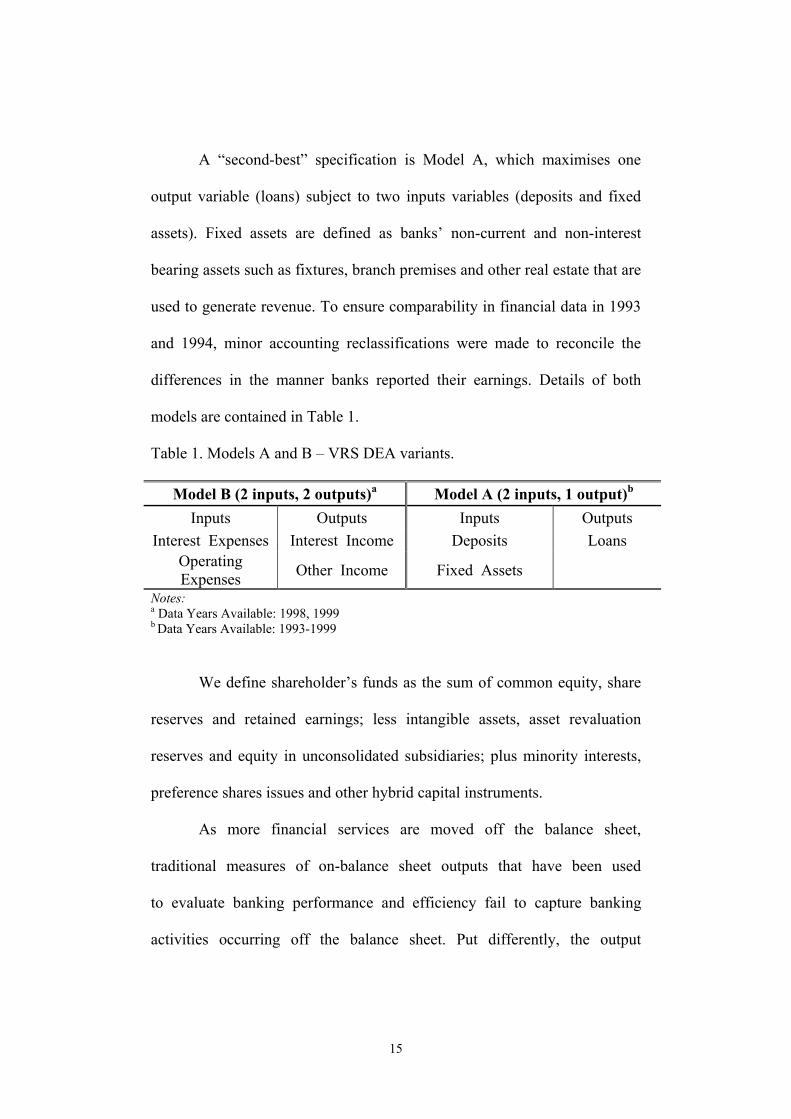
A “second-best” specification is Model A, which maximises one
output variable (loans) subject to two inputs variables (deposits and fixed
assets). Fixed assets are defined as banks’ non-current and non-interest
bearing assets such as fixtures, branch premises and other real estate that are
used to generate revenue. To ensure comparability in financial data in 1993
and 1994, minor accounting reclassifications were made to reconcile the
differences in the manner banks reported their earnings. Details of both
models are contained in Table 1.
Table 1. Models A and B – VRS DEA variants.
Model B (2 inputs, 2 outputs)a Model A (2 inputs, 1 output)b
Inputs Outputs Inputs Outputs Interest Expenses Interest Income Deposits Loans
Operating Expenses Other Income Fixed Assets
Notes: a Data Years Available: 1998, 1999 b Data Years Available: 1993-1999
We define shareholder’s funds as the sum of common equity, share
reserves and retained earnings; less intangible assets, asset revaluation
reserves and equity in unconsolidated subsidiaries; plus minority interests,
preference shares issues and other hybrid capital instruments.
As more financial services are moved off the balance sheet,
traditional measures of on-balance sheet outputs that have been used
to evaluate banking performance and efficiency fail to capture banking
activities occurring off the balance sheet. Put differently, the output

16
variables used in conventional DEA models, like Models A and B, do
not reflect the growth of off-balance sheet (OBS) services.
This leads us to the risk-weighted DEA approach, which
models bank output explicitly in terms of risk-weighted assets. Risk-
weighted assets include OBS items that conventional output variables
such as loans fail to capture. By weighting different asset classes by
risk, the entire spectrum of revenue generating assets can be included
in the model.
In accordance with the Basle convention, assets are weighted
according to their inherent level of risk. Five weights - zero, 10%,
20%, 50% and 100% - are assigned to five broad asset classes.
Relatively risk free assets like cash, claims on sovereigns, central
banks and OECD governments are assigned zero weighting. Securities
issued by governments are assigned a 10-20% weight, depending on
the residual time to maturity. Similar weights apply to loans
guaranteed by multilateral agencies, public sector agencies and
sovereigns.
Claims to the private sector with a residual maturity of over
one year, both in the form of commercial loans and securities, are
assigned 100% weights on account of relative credit and investment
risk. Full risk weights also apply to premises, real estate, investment
securities (corporate shares and bonds) and other fixed assets.

17
Contingent liabilities that substitute for loans like general loan
guarantees, bank acceptance guarantees and standby letters of credit for
loans and securities will carry a 100% risk weight. However, transaction and
trade-related contingencies (bid bonds, warrants and credits guaranteed by
shipment performance bonds) will receive a lower 20-50% weight,
depending on tenure. Shorter-term commitments or commitments which
can be unconditionally cancelled at any time carry only low risk and
therefore a nil weight.
Table 2. Model C (2 x 1 DEA – VRS)
Inputs Outputs Deposits Risk Weighted Assets
Fixed Assets Notes: Aim: Cross-temporal Comparison. Reference Years: 1993, 1994, 1998, 1999
In Model C presented in Table 2, risk-weighted assets are
explicitly regarded as the sole bank output, while inputs are
represented by deposits and fixed assets as in Model A. From the
same set of audited financial statements, it was possible to calculate
risk weighted assets for banks in 1993, 1994, 1998 and 1999, thus
enabling us to track efficiency changes over the same reference period
as before.
Model C is a distinct improvement over Model A for three
reasons. First, risk-weighted assets are a better output proxy than
loans as the former includes OBS items. Relative efficiency is likely

18
to be significantly different when we take into account potential
economies of scope between the swaps and forward books. Second, as
risk-weighted assets encompass the entire spectrum of a bank’s
earning assets (e.g. securities, loans, investments and OBS items),
Model C offers a more realistic abstraction of the bank’s revenue
function than either A or B. Third, using risk-weighted assets instead
of interest income or non-interest income as an output proxy allows
us to avoid the problem of variations in product prices across banks.
This is an area of concern for users of Model B.
Nonetheless, the risk-weighted asset approach may require a
higher degree of financial disclosure that may exceed statutory
requirements in many jurisdictions. This is especially relevant in the
context of developing countries. In cases where information is lacking,
the assignment of weights for risk assets falls largely on analyst
discretion.
6. ANALYSIS OF EMPIRICAL RESULTS
The major empirical objective of this paper is to investigate the
properties of DEA scores over time. In order to achieve this
objective, we employ the longitudinal efficiency analysis approach
used in Barr et al (1999) in their study of US banks. In broad terms,
this involves sorting derived DEA scores into quartiles and observing

19
how these quartiles interact with traditional indicators of performance
and model variables.
In accordance with model specifications set out in Tables 1
and 2, we estimated the data using three alternative DEA models.
Score trends and descriptive statistics are presented in Figure 1 and
Table 3 respectively.
Figure 1. Mean scores by DEA model.
0.00
0.20
0.40
0.60
0.80
1993 1994 1995 1996 1997 1998 1999
Tech
nica
l Effi
cien
cy S
core
s
Model B - Interest Inc/exp Model A - Loans Model C - RWA

20
Table 3. Descriptive Statistics for the Average Efficiency Scores by DEA Model
Model Ca Model Bb Model Aa
Mean Score 0.437 0.533 0.332 Standard Error 0.023 0.064 0.030 Median 0.436 0.512 0.302 Standard Deviation 0.133 0.352 0.178 Sample Variance 0.018 0.124 0.032 Kurtosis 0.752 -1.465 -0.553 Skewness 0.684 0.090 0.798 Range 0.598 0.987 0.600 Minimum 0.221 0.014 0.128 Maximum 0.819 1.000 0.728 Sample Size 35 30 35
Spearman Rank-Order Correlation Model C Model B Model A Model C (2x1) 1.00 - - Model B (2x2) - 0.69 1.00 - Model A (2x1) 0.28 - 0.34 1.00 Notes: a Models A and C - Efficiency scores are calculated using 7 years of data for 35 observations and the descriptive statistics are based on the average efficiency for each bank over the study period. b Model B – Efficiency scores are calculated using 2 years of data for 30 observations and the descriptive statistics are based on the average efficiency for each bank over the two-year period.
The seven year range of this study encapsulates significant
changes in economic climate, in which Singapore banks experienced
both difficult and profitable operating periods. 1993-1996 marked a
period of robust growth in financial services output, followed by the
“down” years of 1997 and 1998 and resurgent growth in 1999.
All the models related well to competitive conditions in the
banking industry. In Figure 1, both A and C identified 1997 as the
year with the lowest scores (averaging 0.2), when credit market
conditions in the region deteriorated rapidly. All three models painted

21
a consistent picture of steadily rising efficiency scores between 1997
and 1999. Model B reported a more modest improvement in
efficiency scores than A or C between 1998 and 1999. We attribute
this to the keener competition in the market, which generally meant
that net interest margins were being compressed. Due to the variables
used, this affected Model B to a greater extent than models A and C.
The trends in scores reported by models A and C in Figure 1 appear
to be mutually consistent in the period 1996-99 and related by time lags in
1993-95. Model A, which measures output by loans to non-bank customers,
reports a sharp increase in mean efficiency scores in 1994, when credit
conditions were buoyant. By contrast, Model C uses risk-weighted assets,
which captures a broader spectrum of earning assets, including newer
fee-based financial services occurring off the balance sheet. It is possible
that OBS activities can explain much of the differences in reported
efficiency scores in Models A and C between 1993 and 1996, although we
lack reliable data for a more detailed investigation.
7. RELATIONSHIP BETWEEN EFFICIENCY SCORES AND
BANK INDICATORS
The major empirical objective of this paper is to evaluate the
properties of DEA scores over time. More specifically, we want to
examine how derived DEA efficiency scores interact with traditional
22
measures of profitability, size, risk attitude and soundness. We expect
institutions with higher efficiency scores to differ significantly from
those with lower scores in measurable ways. More efficient banks are
likely to have higher return on average assets (ROAA) and lower
loan-to-asset ratios. Finally, we expect positive correlation between
efficiency scores and financial strength as determined by capital
adequacy ratios.
7.1. Do DEA Score Quartiles Perform as a Consistent Measure
over Time?
To isolate their salient characteristics, the derived DEA efficiency
scores from Model C for each annual cross section were sorted in
descending order and divided into quartiles. In this fashion, we can
examine how the higher score quartiles compare with lower score
quartiles in terms of performance measures and model variables. How
the quartiles interact with these variables over time should indicate if
derived DEA scores are a useful abstraction of reality over time.

23
Figure 2. Score by Efficiency Quartile.
The results indicate that the differences in mean scores
between the most and least efficient quartiles are significant at the
1% level of confidence. This implies that the differences between the
efficiency ranked quartiles are statistically meaningful and that the use
of efficiency quartiles to evaluate DEA technical efficiency scores is
statistically appropriate.
7.2. Does Institution Size Matter?
Another stated goal of this study was to investigate the role played by bank
size in determining efficiency. Quartile analysis provided interesting results.
Figure 3 shows that in six of the seven reference years, banks in the
smallest size quartile (by total assets) had consistently higher mean
technical efficiency scores than the largest size quartile. Consistent
with Barr et al (1999), scores from our model also highlight the
0.00
0.20
0.40
0.60
0.80
1.00
1993 1994 1995 1996 1997 1998 1999
Effic
ienc
y Sc
ore
Most Efficient 2nd Quartile 3rd Quartile Least Efficient

24
potential for greater inefficiencies in the operation of larger and more
complex banking operations. This also implies that despite the
differences in variables used, scores obtained from both DEA models
share some common properties.
Figure 3. Efficiency score by size Quartile.
Economic conditions have a marked impact on the extent of the
differences in efficiency scores between largest and smallest size quartiles.
Thus, the divergence in scores between the largest and smallest size
quartile lines in Figure 3 appeared to be at its widest between 1993 and
1994, during which period the banking industry experienced robust asset
growth. This gap narrowed progressively after 1997, which coincided with
the onset of a sharp deceleration in loan advances and economic growth
rates.
0.10
0.30
0.50
0.70
1993 1994 1995 1996 1997 1998 1999
Effic
ienc
y Sc
ore
Largest 2nd Quartile 3rd Quartile Smallest

25
7.3. Do Mergers Improve Efficiency Scores?
Table 4 summarises the DEA scores for two cases of mergers identified in
Singapore following the Avkiran (1999: 1006) approach. In each case, we
compared the ranking of the entity in the sample implied by its DEA
technical efficiency score in the period before and after merger.
Table 4. Relative Efficiency Scores Pre- And Post-Merger – Model C Scores.
Merged Institution Year Constituent A Constituent B Case 1 Keppel Tatlee Bank Keppel Bank Tat Lee Bank 1993 0.25 (Rank: 32/32) 1.00 (Rank: 7/32) 1994 0.81 (Rank:6/33) 0.17 (Rank: 30/33) 0.21 (Rank: 28/31) 1997 0.08 (Rank: 15/30) 1998 1.00 (Rank: 4/30) 1999 Case 2 Bank of Tokyo-
Mitsubishi Bank of Tokyo Mitsubishi Bank
1993 0.52 (Rank: 18/32) 0.27 (Rank: 30/32) 1994 0.85 (Rank: 5/33) 0.20 (Rank 26/33) 0.77 (Rank: 9/28) 1996 0.24 (Rank: 26/31) 1997 0.05 (Rank: 19/30) 1998 0.39 (Rank: 16/30) 1999
In Case 1, although efficiency rankings based on DEA scores had
improved steadily between 1997 and 1999, the merged entity was
ranked lower in the first two years relative to one of its constituents
(Keppel Bank) in the years before merger. In Case 2, one of the
constituent banks (Bank of Tokyo) before merger had generally higher
efficiency rankings than the merged Singapore unit of the Bank of
Tokyo-Mitsubishi. In both cases, DEA efficiency rankings for the merged

26
banks are not always unambiguously better off than their constituents before
merger. Neither of the two mergers produced banks large enough to control
a dominant share of the market.
Overall, this exercise provided no conclusive evidence to support the
hypothesis that merged financial institutions in the Singaporean context
could at least maintain their pre-merger level of efficiency (based on DEA
scores).These findings are consistent with Avkiran (1999), who found that
acquiring banks could not always maintain pre-merger relative efficiency
rankings.
7.4. Are Banks with Higher Efficiency Scores More Profitable?
Figure 4. ROAA by Efficiency Quartile.
The results suggest that ROAA is generally positively related
to our measure of efficiency. Banks in the highest efficiency quartile
reported higher mean ROAA than banks in the lowest efficiency
-1.0
0.0
1.0
2.0
3.0
1993 1994 1995 1996 1997 1998 1999
Ret
urn
on A
vera
ge A
sset
s, %
Most Efficient 2nd Quartile 3rd Quartile Least Efficient
27
quartile in all years other than 1995 and 1998. With the exception of
1995 and 1997, the differences in mean ROAA between the most and
least efficient quartiles in all other years were significant at the 5%
level.
In Figure 4, the ROAA trends for the respective score quartiles
are not rank distinct. Rank distinction is harder to achieve in quartile
based studies using smaller samples due to the “outlier” problem. This
phenomenon is also responsible for the general lack of smoothness in
the trends in Figure 4. Barr et al (1999) were able to achieve rank
distinction as a result of the relatively large sample used (which tends
to mitigate the effects of data “outliers”). Another factor relates to the
differences in model variables used. Since risk-weighted assets is a proxy
for output (unlike interest income in Barr et al), we are not surprised
to find a less direct linkage between the efficiency scores and
industry measures of profitability.
ROAA appears to be a good indicator of the impact of
varying economic conditions on the different efficiency quartiles. At
the height of the financial crisis in 1998, mean ROAA for the most
efficient quartile dropped to a low of –0.76%. This suggests that the
banks with the higher efficiency scores had either sought to make full
provisions for possible loan loss charges early or had simply written
off bad assets ahead of their peers. If this is true, then this argument

28
would also corroborate the sharp rebound in ROAA for the most
efficient quartile in the subsequent year.
7.5. Are Banks with Higher Efficiency Scores More Risk Averse?
Figure 5. Mean loan/assets by Efficiency Quartile.
In the context of US banks, Barr et al (1999) found that less
efficient banks had higher loan asset ratios, which they interpreted as
an indication of lower risk aversion. However, implicit in their inference is
that the loan-to-asset ratio accurately portrays the attitude of a bank towards
risk. It can be readily argued that a simple ratio like the loan-asset ratio is
unlikely to capture fully a bank’s attitude towards risk. A glaring
omission, for instance, is OBS activity, which typically exceeds the
on-balance sheet assets of major commercial banks operating in
Singapore.
0
20
40
60
1993 1994 1995 1996 1997 1998 1999
Tota
l loa
ns/T
otal
Ass
ets,
%
Most Efficient 2nd Quartile 3rd Quartile Least Efficient

29
With the exception of 1995, the highest efficiency score quartile had
lower loan-asset ratios than the lowest score quartile on average. This is
evident from Figure 5. This finding may be interpreted in two conflicting
ways. First, as Barr et al (1999) suggested, this could simply imply
that less efficient banks (which tend to be less profitable) have a
tendency to enhance profit margins by adopting higher credit risk
profile. This means that more efficient banks are therefore more risk
averse. On the other hand, it is also possible to show that more
efficient banks can be less averse to risk, despite higher ROAAs and
lower loan-asset ratios. For instance, these banks may have higher
levels of OBS businesses (eg. fee-based and speculative activity like
foreign exchange derivatives and contingent liabilities), which generate
greater profitability and which the loan-asset ratio fails to capture.
7.6. Are Banks with Higher Efficiency Scores “Stronger” Institutions?
Figure 6. Mean capital adequacy ratio by Efficiency Quartile.
0
10
20
30
1993 1994 1995 1996 1997 1998 1999
Mea
n C
AR
, %
Most Efficient 2nd Quartile 3rd Quartile Least Efficient

30
There is a noticeable tendency for banks with higher efficiency
scores to have “stronger” capital structures measured in terms of the
capital adequacy ratio (CAR). With the exception of 1998, a clear
positive relationship exists between the CAR and efficiency scores for
the duration of our study. However, this relationship does not seem to
be independent of economic conditions. In Figure 6, the “most-to-
least-efficient” differences narrow significantly during the difficult
years of 1997 and 1998. Another possible factor explaining the drop
in the mean CAR of more efficient banks was that Singapore’s CAR
requirements were modified in December 1998 to reduce the
minimum Tier 1 capital requirement from 12% to 10%, and to allow
for Upper Tier 2 capital to be used as regulatory capital for the
remaining 2%.
These findings are consistent with Barr et al (1999), who also found
evidence of a significant positive relationship between bank efficiency and
bank examiner ratings (measured by the CAMELS rating1). This suggests
that DEA models can be employed by regulators and banks as an “off-site”
monitoring and internal benchmarking device.
1 A CAMELS rating is a confidential six-part composite rating and the outcome of an on-site examination of a bank by the US Federal Reserve. The overall rating is divulged to the management of the bank, but component ratings are withheld by regulators. The CAR is an integral component of the rating.

31
7.7. Relationship Between Efficiency Scores and Model Variables.
Barr et al (1999) have observed that some of these differences would
also manifest themselves in the input and output variables of the
model. Nonetheless, we do not expect clearer patterns of causality between
efficiency scores and specific input and output variables per se. This is
perhaps because reported DEA efficiency scores reflect the firms’ relative
ability to maximise output variables, given its inputs.
7.8. Risk Weighted Assets
Figure 7. Risk weighted assets by Efficiency Quartile.
RWA are broadly indicative of the level of earning assets or
the ability of financial institutions to generate revenues. In tandem
with expectations, it can be observed in Figure 7 that the highest score
quartile has significantly higher levels of RWA (relative to assets) than the
lowest score quartile in all years except 1996. This implies a positive
0
3
6
9
12
1993 1994 1995 1996 1997 1998 1999
RW
Ass
ets/
Tota
l Ass
ets,
(tim
es)
Most Efficient 2nd Quartile 3rd Quartile Least Efficient

32
relationship between efficiency scores and the mean RWA-to-total-asset
ratio, although clear rank distinction between the mean RWA levels of
different score quartiles was not achieved2.
7.9. Deposits
The longitudinal interaction between the mean adjusted deposits of the most
and least efficient quartiles is more difficult to characterise. We had
expected a tendency for efficiency scores to relate negatively to
deposits as a percentage of assets, since deposits are an input variable
in the model. However, as evident in Figure 8, no meaningful
relationship may be inferred.
Figure 8. Mean adjusted deposits by Efficiency Quartile.
2 This was largely due to outliers in the data. While we had removed the extreme observations from the sample, the variation in mean RWA/total assets between observations remained large.
0.0
20.0
40.0
60.0
80.0
1993 1994 1995 1996 1997 1998 1999
Dep
osits
/Tot
al A
sset
s, %
Most Efficient 2nd Quartile 3rd Quartile Least Efficient

33
The results also suggest that the ratio of deposits to assets of the
efficiency quartiles move independently with economic conditions over
time. However, taking averages for the quartiles, one finds declining
mean deposits as a percentage of total assets between 1993 and 1996,
but a steady rising trend after 1996. This seems to concur with industry
characteristics. Average growth in aggregate loans (16.44%) had
outstripped deposits (10.82%) during the good years (1993-96), but
deposit growth (14.42% versus 5.24%) was relatively higher during the
difficult years (1997-99).
7.10. Fixed Assets
Figure 9. Mean adjusted fixed assets by Efficiency Quartile
We observe no consistent relationship between efficiency scores
and the level of fixed assets in Figure 9, although a general negative
0.0
0.4
0.8
1.2
1.6
1993 1994 1995 1996 1997 1998 1999
Fixe
d A
sset
s/To
tal A
sset
s, %
Most Efficient 2nd Quartile 3rd Quartile Least Efficient

34
trend is noticeable if we limit the comparison to the highest and lowest
score quartiles. It is generally expected that banks with higher
efficiency scores will have lower levels of fixed assets (relative to
assets). In five of the seven years of the sample period, banks with
higher scores had lower levels of fixed assets (relative to assets).
Whereas the trend between 1994 and 1998 is consistent with
expectations, the reverse is true for the years 1993 and 1999.
8. CONCLUDING REMARKS
Despite our best efforts, data constraints remained the largest impediment to
the study. For instance, a broader and deeper sample base would have
enabled us to experiment more rigorously with a larger number of
alternative DEA model specifications. Limited by a maximum size of 35
observations in each of the seven annual cross-sections, a 1x2 functional
form seemed appropriate. While shortcomings have been alleviated by our
usage of novel OBS-inclusive variables like RWA, we would also have
liked to expand Model C into a larger functional form, incorporating income
statement variables, like interest income and interest expense, with risk-
weighted assets. Unfortunately, public access to key income statement
variables only became available after 1998. Not only should these general
refinements result in smoother trends in the quartile-based studies, but we
also expect to attain rank distinction in the quartile based analysis with the

35
same regularity that US-based researchers using large samples have been
able to achieve.
Another concern relates to the inclusion of non-performing loans
(NPL), which could potentially have significant impact on calculated
efficiency scores and implied rankings. Based on the time trend of
aggregate NPLs in the banking system, this impact is likely to be most
apparent between 1997 and 1999. We would also have expected to
establish a negative relationship between the percentage of gross loans
that are non-performing and the efficiency score quartiles in
accordance with Barr et al (1999)
A possible extension to this study is the Malmquist DEA
technique, which uses pooled time series data to calculate changes in
total factor productivity (TFP), technological effects, technical efficiency
and allocative efficiency. Färe et al (1994) extended the Malmquist index
of the TFP growth approach to illustrate how component distance
functions can be estimated using DEA-like formulations. The resulting
TFP indices could be decomposed into technical change and technical
efficiency change components. Nonetheless, this represents a significant
departure from our stated objectives, which focused on examining the
relationships between traditional measures of bank efficiency and DEA
efficiency scores.

36
In summarising the results of the analysis of Singapore bank
efficiency, several points should be emphasised. We sought to evaluate
the properties of DEA scores over time, using the longitudinal
analysis approach of Barr et al (1999). Essentially, efficiency scores
were sorted into quartiles and tested against traditional indicators of
bank performance and with the input-output variables of our model.
To varying degrees, the results indicate significant relationships between
efficiency scores and traditional indicators of bank performance, namely
capital adequacy, profitability, loan-to-asset ratio and institution size.
Subsequently, we found evidence to support a positive association
between scores and the output variable, but not between scores and
the input variables.
While it is imperative that users understand its limitations,
DEA models can offer much potential for a significant advance in the
comparative analysis of financial institutions by enabling the
concurrent study of the multiple variables that affect bank efficiency
over time. DEA models could be employed to develop industry
monitoring tools using time series data for policy inference and
performance evaluation. For industry analysts, DEA offers a
multifaceted ranking methodology for benchmarking based on a priori
economic reasoning, i.e. the efficiency measurement insights of Farrell
(1957). This represents a significant improvement over traditional single

37
ratio-driven rankings. In the absence of superior ranking alternatives, we are
obliged by necessity and not choice to adhere to the present DEA
methodology, given our data limitations.
ACKNOWLEDGEMENTS
The opinions expressed in this paper do not necessarily reflect the views of
the Singapore Ministry of Trade and Industry. The preliminary empirical
work for this paper was undertaken by Wai Ho Leong at Melbourne
University. The authors would like to thank an anonymous referee for
helpful comments on an earlier draft of the paper.

38
REFERENCES
Avkiran, N. (1999). “The evidence on efficiency gains: The role of mergers
and the benefits to the public”, Journal of Banking and Finance, 23,
pp. 991-1013.
Banker, R., A. Charnes, and W. Cooper (1984). “Some models for
estimating technical and scale inefficiencies in data envelopment
analysis”, Management Science, 30, pp. 1078–1092.
Barr, R., K. Killgo, T. Siems, and S. Zimmel, (1999). “Evaluating the
productive efficiency and performance of US commercial banks”,
Financial Industry Studies Working Paper, No. 99-3, Federal Reserve
Bank of Dallas, Dallas.
Bauer, P., A. Berger, G. Ferrier, and D. Humphrey (1997). “Consistency
conditions for regulatory analysis of financial institutions: A
comparison of frontier efficiency methods”, US Federal Reserve
Financial Services, Working Paper No. 02(97).
Berger, A. and D. Humphrey (1991). “The dominance of inefficiencies over
scale and product mix economies in banking”, Journal of Monetary
Economics, 28, pp. 117–148.
Berger, A. and D. Humphrey (1992). “Measurement and efficiency issues in
commercial banking”, in Z. Griliches (ed.), Output Measurement in
the Service Sectors, The University of Chicago Press, Chicago

39
Berger, A. and D. Humphrey (1997). “Efficiency of financial institutions:
International survey and directions for future research”, European
Journal of Operational Research, (Special issue). URL:
http://papers.ssrn.com/sol3/papers.cfm?abstract_id=2140 [consulted 4
April 2004].
Berger, A., W. Hunter, and S. Timme (1993). “The efficiency of financial
institutions: A review and preview of research past, present and
future”, Journal of Banking and Finance, 17, pp. 221–249.
Colwell, R. and E. Davis (1992). “Output and productivity in banking”,
Scandinavian Journal of Economics, 94, pp.111–129.
Färe R., S. Grosskopf, M. Norris, and Z. Zhang (1994). Production
Frontiers, Cambridge University Press, Cambridge
Farrell, M. (1957). “The measurement of productive efficiency”, Journal of
the Royal Statistical Society, Series A (General) 120, pp. 253–289.
Favero, C. and L. Papi (1995). “Technical efficiency and scale efficiency
in the Italian banking sector: A non-parametric approach”,
Applied Economics, 27, pp. 385–395.
Fecher, F. and P. Pestieau (1993). “Efficiency and competition in OECD
financial services”, in H. Fried, C. Lovell, and S. Schmidt (eds.), The
measurement of productive efficiency: techniques and applications,
Oxford University Press, UK

40
Ferrier, G. and C. Lovell (1990). “Measuring cost efficiency in banking:
Econometric and linear programming evidence”, Journal of
Econometrics, 46, pp. 229–245.
KPMG (1997). Survey of banking and financial institutions in Singapore,
KPMG Peat Marwick Consultants, Singapore.
Leibenstein, H. and S. Maital (1992). “X-efficiency after a quarter of a
century: empirical estimation and partitioning of X-efficiency. A data
envelopment analysis approach”, American Economic Review, 82(2),
pp. 428-433
Pi, L. and S. Timme (1993). “Corporate control and bank efficiency”,
Journal of Banking and Finance, 17, pp. 515–530.
Sherman, H. and F. Gold (1985). “Bank branch operating efficiency:
Evaluation with data envelopment analysis”, Journal of Banking and
Finance, 9, pp. 279–315.
Worthington, A. (1998). “The determinants of non-bank financial institution
efficiency: A stochastic cost frontier approach”, Applied Financial
Economics, 8, pp. 279–289.