Wages, Prices, and Labor Markets before the Civil War Wages, Prices, and Labor Markets before the Civil War Claudia Goldin and Robert A. Margo 2.1 Economic Development, Nominal Wage

This PDF is a selection from an out-of-print volume from the National Bureauof Economic Research

Volume Title: Strategic Factors in Nineteenth Century American EconomicHistory: A Volume to Honor Robert W. Fogel

Volume Author/Editor: Claudia Goldin and Hugh Rockoff, editors

Volume Publisher: University of Chicago Press

Volume ISBN: 0-226-30112-5

Volume URL: http://www.nber.org/books/gold92-1

Conference Date: March 1-3, 1991

Publication Date: January 1992

Chapter Title: Wages, Prices, and Labor Markets before the Civil War

Chapter Author: Claudia Goldin, Robert A. Margo

Chapter URL: http://www.nber.org/chapters/c6958

Chapter pages in book: (p. 67 - 104)

2 Wages, Prices, and Labor Markets before the Civil War Claudia Goldin and Robert A. Margo

2.1 Economic Development, Nominal Wage Flexibility, and Antebellum Labor Markets

America experienced several expansions and contractions in economic activity between its founding and the Civil War. The Embargo of 1807 abruptly ended the export boom of the Napoleonic Wars, a recession followed the War of 1812, there was a panic in 1819, and a crisis in 1825. An expansion in the late 1820s and early 1830s gave way to several downturns; rapid recovery succeeded the first, a minor one in 1837, but the second, in 1839, was more prolonged. Minor contractions in the late 1840s and early 1850s were followed by another downturn in 1857. Associated with most of these expansions and contractions, especially the so-called Panic of 1837 and Panic of 1857, were sharp changes in the price level. While the existence of these fluctuations in economic activity is not in doubt, their severity has been ques- tioned.

There are two opposing views of the antebellum economy. One is that the period was marked by at least one severe depression, from 1839 to 1843, and other lesser recessions. Aggregate economic activity, according to this view, was severely diminished during the downturns, and unemployment was both substantial and prolonged in cities and industrial towns. The other interpreta-

The wage data analyzed in this paper were collected by the Center for Population Economics, University of Chicago. The research assistance of Joseph Hunt and research support from Colgate University are gratefully acknowledged. The authors would like to thank Stanley Engerman, Kevin Hassett, Hugh Rockoff, and the participants at the 1990 NBER-DAE Summer Institute, the 1990 AEA-Cliometrics session, and the Cornell University economic history seminar for com- ments on an earlier draft.

67

68 Claudia Goldin and Robert A. Margo

tion is that antebellum fluctuations were more apparent than real; more often only prices, not quantities, changed. Furthermore, whatever unemployment may have been created did not endure for long; the unemployed, particularly laborers, teamsters, and other unskilled workers, migrated to the countryside and returned to industry when conditions turned more favorable.

According to the proponents of the first view, antebellum price changes are evidence of serious and sustained economic hardship. Price fluctuations could have influenced real magnitudes if the antebellum wage lag was long. Real wages would then have decreased during periods of inflation, such as the mid-1 830s, thereby sparking strikes and union activity. And real wages would have increased during periods of deflation, such as the early 1840s. Thus de- flationary periods would have led to or been associated with unemployment. Labor market adjustment would have occurred largely through changes in employment, a real variable, rather than wages, a nominal variable.

Newspaper and other narrative accounts attest to considerable unemployment in cities following the Embargo of 1807, the Panic of 1837, and especially during the deflation of the early 184Os, and have led one historian to state that “more than half of New York’s craft workers reportedly lost their jobs in the immediate wake of the panic” of 1837.2 Many have claimed that artisans, in particular, were thrown out of employment during the well-known economic crises of 1837, 1839, and 1857, and that unemployment in general was high throughout the 1839 to 1842 period and during 1854 and 1855. But if deflation fostered unemployment, inflation must have caused strikes and other union activity, as many have documented for the mid-1830s and, to a lesser extent, in the 1 8 5 0 ~ . ~ The end result-inconstancy of work and dis- tressed labor relations-were, according to many labor histories, the common ground around which working-class life, culture, and politics were shaped, and a dominant element in the emergence of working-class consciousness.4

But according to a revisionist view, even the most severe antebellum price fluctuations had little impact on aggregate real activity and employment. “The parallel between the 1840s and the 1930s,” writes Peter Temin, “extends only to the monetary aspects of the economy. . . . Farmers, textile workers, and

1. See, for example, John R. Commons, et al., History of Labor in the United States (New York, 1916); William Sullivan, The Industrial Worker in Pennsylvania, 1800-1840 (Harrisburg, 1955); Norman Ware, The Industrial Worker, 1840-1860 (New York, 1924); Susan E. Hirsch, Roots of the American Working Class: The Industrialization of Crafts in Newark, 1800-1860 (Philadelphia, 1978); Bruce Laurie, Working People of Philadelphia, 1800-1850 (Philadelphia, 1980); Sean Wilentz, Chants Democratic: New York City and the Rise of the American Working Class. 1788-1850 (New York, 1984); Steven J. Ross, Workers on the Edge: Work, Leisure, and Politics in Industrializing Cincinnati, 1788-1890 (New York, 1985); and Robert W. Fogel, With- out Consent or Contract: The Rise and Fall of American Slavery (New York, 1989).

2. Wilentz, Chants Democratic, p. 294. 3 . Commons, et al., History of Labor; Stanley Lebergott, Manpower in Economic Growth

4. See especially Laurie, Working People; and Wilentz, Chants Democratic. (New York, 1964).

69 Wages, Prices, and Labor Markets before the Civil War

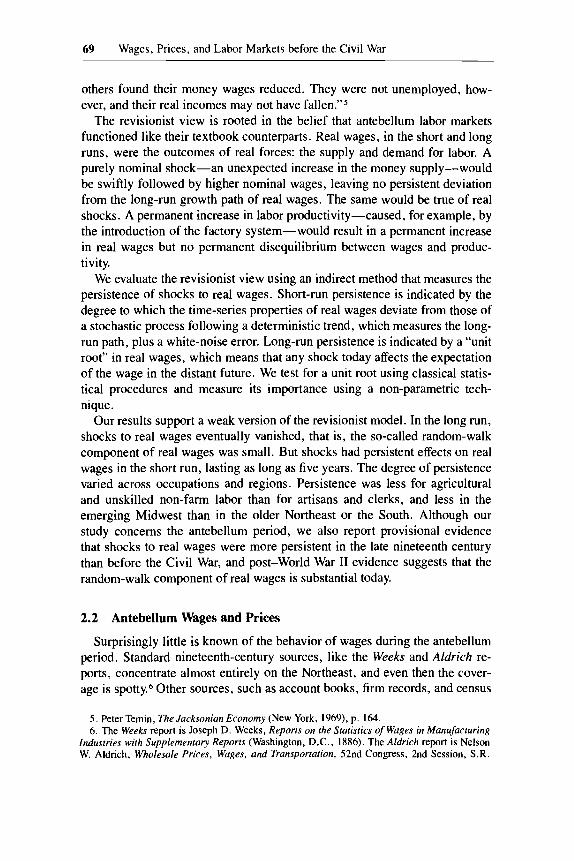
others found their money wages reduced. They were not unemployed, however, and their real incomes may not have fallen.”5

The revisionist view is rooted in the belief that antebellum labor markets functioned like their textbook counterparts. Real wages, in the short and long runs, were the outcomes of real forces: the supply and demand for labor. A purely nominal shock-an unexpected increase in the money supply-would be swiftly followed by higher nominal wages, leaving no persistent deviation from the long-run growth path of real wages. The same would be true of real shocks. A permanent increase in labor productivity-caused, for example, by the introduction of the factory system-would result in a permanent increase in real wages but no permanent disequilibrium between wages and productivity.

We evaluate the revisionist view using an indirect method that measures the persistence of shocks to real wages. Short-run persistence is indicated by the degree to which the time-series properties of real wages deviate from those of a stochastic process following a deterministic trend, which measures the long- run path, plus a white-noise error. Long-run persistence is indicated by a “unit root” in real wages, which means that any shock today affects the expectation of the wage in the distant future. We test for a unit root using classical statistical procedures and measure its importance using a non-parametric technique.

Our results support a weak version of the revisionist model. In the long run, shocks to real wages eventually vanished, that is, the so-called random-walk component of real wages was small. But shocks had persistent effects on real wages in the short run, lasting as long as five years. The degree of persistence varied across occupations and regions. Persistence was less for agricultural and unskilled non-farm labor than for artisans and clerks, and less in the emerging Midwest than in the older Northeast or the South. Although our study concerns the antebellum period, we also report provisional evidence that shocks to real wages were more persistent in the late nineteenth century than before the Civil War, and post-World War I1 evidence suggests that the random-walk component of real wages is substantial today.

2.2 Antebellum Wages and Prices

Surprisingly little is known of the behavior of wages during the antebellum period. Standard nineteenth-century sources, like the Weeks and Aldrich reports, concentrate almost entirely on the Northeast, and even then the cover- age is spotty.6 Other sources, such as account books, firm records, and census

5 . Peter Ternin, The Jacksonian Economy (New York, 1969), p. 164. 6. The Weeks report is Joseph D. Weeks, Reporrs on the Statistics of Wages in Manufacturing

Zndustries with Supplementary Reports (Washington, D.C., 1886). The Aldrich report is Nelson W. Aldrich, Wholesale Prices, Wages, and Transportation, 52nd Congress, 2nd Session, S.R.


manuscripts, provide valuable additional information on antebellum wages, but are limited to particular locations, occupations, or time periods.’ We use a new source, the payroll records of civilian employees of the United States Army, which contain wages for various occupations and all parts of the coun- try.8 We assume here that the wage rates apply to the private sector and that the federal government paid workers the “going wage rate.” The assumption is based on the fact that other wages series, derived from a variety of sources, track our series for the periods and regions of o v e ~ l a p . ~

Previous work with the sample yielded annual dollar estimates and indices of nominal daily wages for artisans (blacksmiths, carpenters, machinists, masons, and painters), and laborers (common laborers and teamsters) from 1820 to 1856, for four census regions (Northeast, Midwest, South Atlantic, and South Central). l o We have, in addition, constructed a new series-regional indices of nominal wages of clerks. This wage series is, we believe, the first for a white-collar occupation in the antebellum period. The nominal wage indices are graphed in Figures 2.1 and 2.2 and their numerical values are reported in Appendix A Tables 2A.1 (artisans), 2A.2 (laborers), and 2A.3 (clerks). ’ I

1394 (Washington, D.C., 1893). Philip R. P. Coehlo and James F. Shepherd, “Regional Differ- ences in Real Wages: The United States, 1851-1880,” Explorations in EconomicHistory, 13 (Jan. 1976). p. 205, point out that the Weeks data “exhibit a high degree of variability before 1860, probably due to a scarcity of data for . . . the 1850s.”

7 . See, for example, Robert G. Layer, Earnings of Cotton Mill Operatives, 1825-1914 (Cam- bridge, Mass., 1955); Walter B. Smith, “Wage Rates on the Erie Canal,” Journal ofEconomic History, 23 (Sept. 1963), pp. 298-31 1; Lebergott, Manpower, pp. 257-333; Donald R. Adams, Jr., “Wage Rates in the Early National Period: Philadelphia, 1785-1830,” Journal of Economic History, 28 (Sept. 1968). pp. 404-26; Jeffrey Zabler, “Further Evidence on American Wage Dif- ferentials,” Explorations in Economic History, 10 (Fall 1972). pp. 109-17; Donald R. Adams, Jr., “The Standard of Living During American Industrialization: Evidence from the Brandywine Re- gion, 1800-1860,” Journal of Economic History, 42 (Dec. 1982), pp. 903-17; “Prices and Wages in Maryland, 1750-1850,” Journal ofEconomic History, 46 (Sept. 1986). pp. 625-45; and Ken- neth Sokoloff, “The Puzzling Record of Real Wage Growth in Early Industrial America, 1820- 1860’ (manuscript, University of California, Los Angeles, 1986). See also Kenneth Sokoloff and Georgia Villaflor, chap. 1 in this volume.

8. The collection is known as the “Reports of Persons and Articles Hired, 1818-1905,” Record Group 92, National Archives. For a detailed discussion of the characteristics of the “Reports,” see Robert A. Margo and Georgia C. Villaflor, “The Growth of Wages in Antebellum America: New Evidence,” Journal ofEconomic History, 47 (Dec. 1987), pp. 873-95.

9. See the discussion in Margo and Villaflor, “The Growth of Wages”; also see Robert A. Margo, “Wages and Prices before the Civil War: A Survey and New Evidence,” in Robert E. Gallman and John Wallis, eds., American Economic Growth and the Standard of Living Before the Civil War (Chicago, 1992, forthcoming). Also, Wilentz, Chants Democratic (p. 419, figure 5) has data for masons and laborers in New York City over the 1835 to 1845 period that reasonably track those here for the Northeast.

10. The annual dollar estimates are in Margo and Villaflor, “The Growth of Wages,” pp. 893- 95. The annual indices are presented in Robert A. Margo, “Appendix: The Growth of Wages in Antebellum America,” Colgate University, Department of Economics, Discussion Paper no. 88- 06 (1988).

11. The construction of the annual dollar estimates involves the weighting of within-region wage estimates, while the construction of the indices does not; see Margo and Villaflor, “The

Fig. 2.1 Midwest Regions Notes: 1856 = 100 for all indices. Shaded areas are peak-to-trough periods of the NBER business cycle. The year 1834 begins the series and is a trough year. Sources: See text. See also Appendix Tables 2A. I-2A.4.

Price Indices, and Nominal Wage Indices of Laborers, Artisans, and Clerks, in the Northeast and

Fig. 2.2 Price Indices, and Nominal Wage Indices of Laborers, Artisans, and Clerks, in the South Atlantic and South Central Regions Notes: 1856 = 100 for all indices. Shaded areas are peak-to-trough periods of the NBER business cycle. The year 1834 begins the series and is a trough year. Sources: See text. See also Appendix Tables 2A. 1-2A.4.


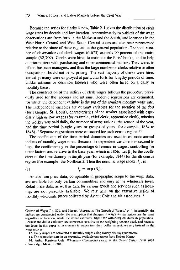
Because the series for clerks is new, Table 2.1 gives the distribution of clerk wage rates by decade and fort location. Approximately two-thirds of the wage observations are from forts in the Midwest and the South, and locations in the West North Central and West South Central states are also over-represented relative to the share of these regions in the general population. The total number of observations of clerk wages (6,673) exceeds 20 percent of the entire sample (32,709). Clerks were hired to maintain the forts’ books, and to help quartermasters with purchasing and other commercial matters. They were, in effect, business managers, and thus the large number of clerks relative to other occupations should not be surprising. The vast majority of clerks were hired annually; many were employed at particular forts for lengthy periods of time, unlike artisans or common laborers who were often hired on a daily or monthly basis.

The construction of the indices of clerk wages follows the procedure previ- ously used for the laborers and artisans. Hedonic regressions are estimated, for which the dependent variable is the log of the nominal monthly wage rate. The independent variables are dummy variables for the location of the fort (for example, St. Louis), characteristics of the worker associated with especially high or low wages (for example, chief clerk, apprentice clerk), whether the worker was paid daily, the number of army rations, the season of the year, and the time period (single years or groups of years, for example, 1834 to 1846). l 2 Separate regressions were estimated for each census region. l 3

The coefficients of the time-period dummies are used to estimate annual indices of monthly wage rates. Because the dependent variable is measured in logs, the coefficients give the percentage difference in wages, controlling for other factors and relative to the base year, which is 1856. Let pji be the coefficient of the time dummy in thejth year (for example, 1844) for the ith census region (for example, the Northeast). Then the nominal wage index, I,,, is

Antebellum price data, comparable in geographic scope to the wage data, are available for only certain commodities and only at the wholesale level. Retail price data, as well as data for various goods and services such as housing, are not presently available. We rely here on the extensive series of monthly wholesale prices collected by Arthur Cole and his associates. l4

Growth of Wages,” p. 879, and Margo, “Appendix: The Growth of Wages,” p. 4. Essentially, the indices are constructed under the assumption that changes in wages within regions are the same regardless of location, while the dollar estimates adjust for within-region shifts in population. Because the dollar estimates are somewhat sensitive to the weighting scheme used, and because our focus in this paper is on changes in wages (not their dollar values), we rely instead on the wage indices.

12. Daily wages are converted to monthly wages using twenty-six days per month. 13. The regressions are in an appendix, available on request from Robert Margo. 14. Arthur Harrison Cole, Wholesale Commodity Prices in rhe Unired Stares, 1700-1861

(Cambridge, Mass., 1938).


Table 2.1 Distribution of the Wage Rate Sample for Clerks, by Decade and Fort Location

Percent of Number Aggregated Total

Northeast 1821-30

1841-50 I83 1-40

185 1-56

Southern New England Northern New England New York City Upstate New York Philadelphia Carlisle, Pennsylvania Washington, D.C. Baltimore

Total

1821-30 I83 1-40

Midwest

1841-50 185 1-56

Ohio, Western Pennsylvania Illinois, Indiana Michigan, Iowa, Wisconsin Minnesota Kansas Missouri

Total South Atlantic

1821-30

1841-50 I85 1-56

Virginia South Carolina Georgia Florida

Total South Central

1821-30 1831-40

183 1-40

184 1-50 1851-56

Kentucky, Tennessee Mississippi Arkansas

399 596

1,022 376

265 68

462 133 87 1 I l l 222 26 I

2,393

378 758 486 267

344 153 351 99

296 967

1,889

198 534 245 112

26 1 279 258 29 I

1.089

I67 470 376 289

62 14

317

16.7 24.9 42.7 15.7

11.1 2.8

19.3 5.6

36.4 4.6 9.3

10.9 35.9

20.0 40. I 25.7 14.1

18.2 8.1

18.9 5.2

15.7 51.2 28.3

18.2 49.0 22.5 10.3

24.0 25.6 23.7 26.7 16.3

12.8 36.1 28.9 22.2

4.8 1.1

24.3


Table 2.1 (continued)

Percent of Number Aggregated Total

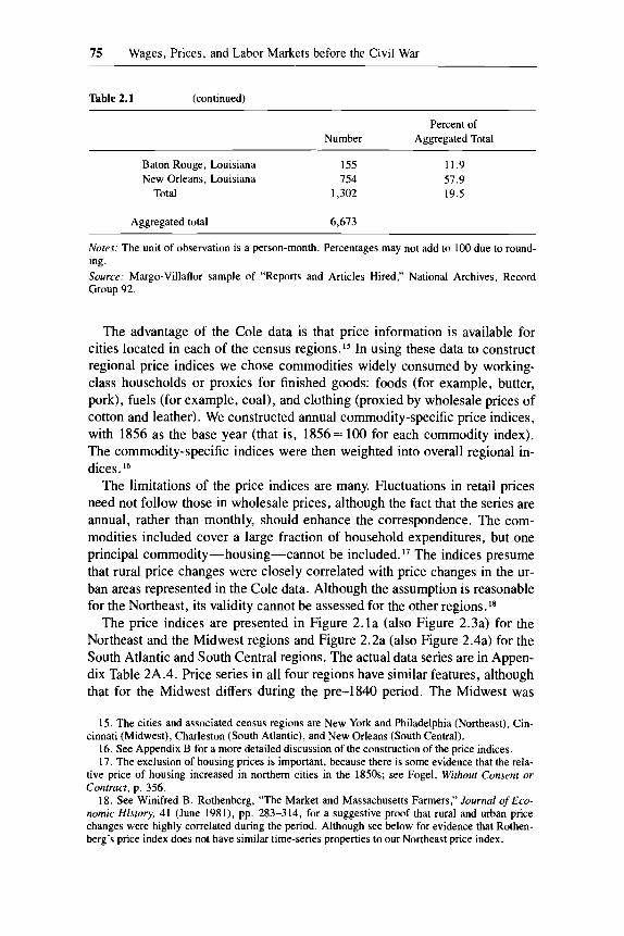
Baton Rouge, Louisiana 155 11.9 New Orleans, Louisiana 154 51.9

Total 1,302 19.5

Aggregated total 6,673

Notes: The unit of observation is a person-month. Percentages may not add to 100 due to round- ing. Source: Margo-Villaflor sample of “Reports and Articles Hired,” National Archives, Record Group 92.

The advantage of the Cole data is that price information is available for cities located in each of the census regions.I5 In using these data to construct regional price indices we chose commodities widely consumed by working- class households or proxies for finished goods: foods (for example, butter, pork), fuels (for example, coal), and clothing (proxied by wholesale prices of cotton and leather). We constructed annual commodity-specific price indices, with 1856 as the base year (that is, 1856= 100 for each commodity index). The commodity-specific indices were then weighted into overall regional indices. l6

The limitations of the price indices are many. Fluctuations in retail prices need not follow those in wholesale prices, although the fact that the series are annual, rather than monthly, should enhance the correspondence. The commodities included cover a large fraction of household expenditures, but one principal commodity-housing-cannot be included. The indices presume that rural price changes were closely correlated with price changes in the urban areas represented in the Cole data. Although the assumption is reasonable for the Northeast, its validity cannot be assessed for the other regions.’*

The price indices are presented in Figure 2.la (also Figure 2.3a) for the Northeast and the Midwest regions and Figure 2.2a (also Figure 2.4a) for the South Atlantic and South Central regions. The actual data series are in Appen- dix Table 2A.4. Price series in all four regions have similar features, although that for the Midwest differs during the pre-1840 period. The Midwest was

15. The cities and associated census regions are New York and Philadelphia (Northeast), Cin-

16. See Appendix B for a more detailed discussion of the construction of the price indices. 17. The exclusion of housing prices is important, because there is some evidence that the rela-

tive price of housing increased in northern cities in the 1850s; see Fogel, Without Consent or Contract, p. 356.

18. See Winifred B. Rothenberg, “The Market and Massachusetts Farmers,” Journal of Eco- nomic History, 41 (June 1981). pp. 283-314, for a suggestive proof that rural and urban price changes were highly correlated during the period. Although see below for evidence that Rothen- berg’s price index does not have similar time-series properties to our Northeast price index.

cinnati (Midwest), Charleston (South Atlantic), and New Orleans (South Central).


growing rapidly from 1820 to 1840 but did not become integrated into the national market for goods until around mid-century. l9

All four price series have numerous oscillations around a generally declining trend. There are two large deviations, one considerably larger than the other. The first is the well-known inflation of the post-1834 period with the subsequent collapse during 1837 and the rapid deflation from 1839 to 1842. Prices rose between 25 and 45 percentage points, depending on the region, during the 1834 to 1836/37 period and then plummeted by well over 40 percentage points during the deflation. Prices began a secular upward trend after 1842, with a spike in 1847 followed by a substantial decline and then continued increase during the years following the California gold rush. Except in the Midwest, where prices rose 19 percent from the 1820s to the 1850s, the long-term trend in prices was basically flat or slightly downward.

The nominal wage indices for the three occupational groups-laborers (including teamsters), artisans, and clerks-are shown in the remaining panels of Figure 2.1 for the Midwest and Northeast regions, and in Figure 2.2 for the South Atlantic and South Central regions. The series for laborers and artisans have been examined in detail elsewhere, and we summarize that discussion here. 2o

In the Northeast and Midwest, laborer (nominal) wages are level to around 1835. They spike, first up and then down, just after 1835, and then display an upward movement to 1856. In contrast, laborer wages in the South Atlantic first decline, then spike up and down in the 1830s, and end with a decade of virtual stability. Those of the South Central region have upward and downward movement throughout with no apparent tendency to mimic the price data.

The artisan wage series appears distinct from that for laborers in most of the regions. In the Midwest, for which the artisan and laborer series seem most similar, there are two spikes in the 1830s with secular growth before and after. But in the Northeast, while the general trend is similar to that for laborers, the large changes in the 1830s are absent. Oscillations in the South Cen- tral data are more numerous than in the laborer data, although the largest is during the period of greatest price fluctuation. The South Atlantic artisan data display no apparent relationship to the laborer data nor to the price series.

Indices of clerk wages are shown in Figure 2. Id for the Midwest and North- east, and in Figure 2.2d for the South Atlantic and South Central regions (see also Appendix Table 2A.3). In the Northeast and Midwest, clerk wages grew more or less continuously during the entire period with no obvious relationship to the price series. In the two southern regions, however, wages increase and then decrease during the 1830s. But the two southern series deviate before the 1830s: South Central wages rise while those of the South Atlantic fall.

19. See, for example, Thomas Senior Berry, Western Prices before 1861, Harvard Economic

20. See Margo and Villaflor, “The Growth of Wages in Antebellum America.” Studies, vol. 74 (Cambridge, Mass., 1943).


In general, nominal wages of clerks increase more rapidly in the 1840s than wages of artisans or laborers. As a result, the average annual growth rate of clerk wages (1 820 to 1856) exceeds that for other occupations, and differences are especially large in the South. Previous work with the wage sample for artisans and laborers found no evidence of a surge in skill differentials-the ratio of artisan to unskilled wages-after 1820, as others have claimed.21 That conclusion, however, must now be modified, because it appears that the wages of clerks, who were highly skilled, did grow more rapidly than wages of skilled or unskilled labor during the late antebellum period.22

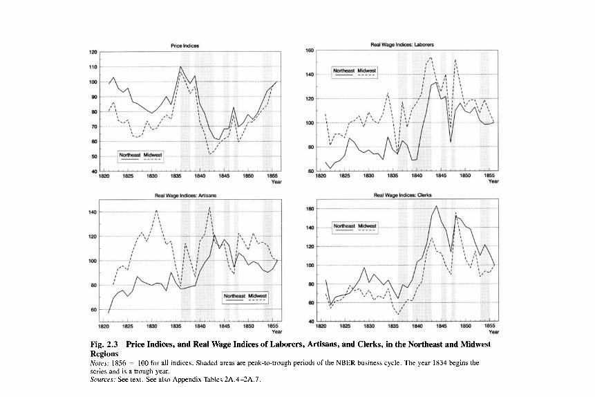
Indices of real wages, based on the nominal wage and price indices, are presented in Figures 2.3 and 2.4 (also Appendix Tables 2A.5 to 2A.7). Real wages grew most among clerks, and they grew more rapidly in the North than the South. Real wages grew less in the newly settled Midwest than in the established Northeast, but the opposite holds when comparing the South Cen- tral and South Atlantic states. In every region real wages grew slowly during the 183Os, increased rapidly in the 1840s, and then decreased in the 1850s.

Real wages of artisans increased by 8 percent from the 1820s to the 1830s in the Northeast, compared with only 3 percent in the Midwest. Real wages continued to rise more rapidly in the Northeast than in the Midwest in the 1840s, before falling in both regions in the 1850s. Over the entire period, real wages of artisans rose at an average annual rate of 0.8 percent per year in the Northeast but at only 0.2 percent per year in the Midwest. Among common laborers and teamsters, real wage growth was similarly slow during the 183Os, but in both regions real wages rose rapidly in the 1840s before falling somewhat in the 1850s. Across the entire 35-year period, however, real wages of unskilled labor in the North grew more rapidly than did the real wages of artisans.23

21. The claim was originally made by Jeffrey Williamson and Peter Lindert, American Inequal- iryc A Macroeconomic History (New York, 1980), pp. 67-75. Evidence against the surge hypothesis-that skilled wages grew more rapidly than unskilled wages-is presented in Margo and Villaflor, “The Growth of Wages,” pp. 883-88.

22. This result is consistent with that in Richard Steckel, “Poverty and Prosperity: A Longitu- dinal Study of Wealth Accumulation, 1850-1860 (manuscript, Department of Economics, Ohio State University, 1988), p. 12. Steckel finds that, in terms of relative wealth, white-collar workers improved their economic position compared with blue-collar or unskilled workers during the 1850s.

23. When the price indices are applied to the annual dollar estimates of skilled and unskilled wages in Margo and Villaflor, “The Growth of Wages,” pp. 893-94, the following annual growth rates (1821-30 to 185 1-56) of real wages are obtained:

Skilled Unskilled

Northeast 0.9 1.2 Midwest 0.4 1.1 South Atlantic 0.5 0.3 South Central 0.7 1 .o

These growth rates are similar to those in Appendix A, except for those in the Midwest which are higher. This difference is a consequence of the weighting procedure used in the construction of the dollar estimates; see Margo, “Appendix: The Growth of Wages,” p. 24.

YBY

Fig. 2.3 Regions Nares: 1856 = 100 for all indices. Shaded areas are pea!-to-trough periods of the NBER business cycle. The year 1834 begins the series and is a trough year. Sources: See text. See also Appendix Tables 2A.4-2A.7.

Price Indices, and Real Wage Indices of Laborers, Artisans, and Clerks, in the Northeast and Midwest

Fig. 2.4 Price Indices, and Real Wage Indices of Laborers, Artisans, and Clerks, in the South Atlantic and South Central Regions Notes: 1856 = 100 for all indices. Shaded areas are peak-to-trough periods of the NBER business cycle. The year 1834 begins the series and is a trough year. Sources: See text. See also Appendix Tables 2A.4-2A.7.


Real wages of artisans in the South Atlantic region increased in the late 1820s but fell sharply in the late 1830s, so that on average real wages were no higher in the 1830s than in the 1820s. As in the two northern regions, real wages rose in the 1840s before falling in the 1850s. Real wages of artisans in the South Central states did not increase on average from the 1820s to the 1830s, but they rose in the 1840s before falling in the 1850s. Overall, real wages grew more rapidly in the South Central states than the South Atlantic states, opposite to the pattern in the northern regions. Real wages of common laborers and teamsters in the South Atlantic states fell 14 percent from the 1820s to the 1830s, rose sharply in the early 1840s, before falling 18 percent in the 1850s from the 1840s average. In the South Central states, real wages of unskilled labor grew by 2 percent from the 1820s to the 1830s and rose by 33 percent in the 1840s, before falling slightly in the 1850s. Over the entire period, real wages of unskilled labor rose at 1 .O percent per year in the South Central states, but the growth rate was negative ( - 0.08 percent per year) in the South Atlantic states.

The real wages of clerks in the Northeast and South Central states were higher in the 1830s than in the 1820s, but the opposite was true in the Midwest and South Atlantic regions. In every region the real wages of clerks increased markedly in the 1840s, before falling again in the 1850s. On average, clerks experienced the greatest real wage growth among the three occupational groups across the entire 35-year period.

One feature of the six real-wage graphs in Figures 2.3 and 2.4 is the marked fluctuation in real wages, particularly during the 1840s. Such fluctuations could arise if nominal wages were relatively stable or responded with a lag while prices varied greatly. The question to which we now turn is how rigid nominal wages were across the four regions and among the three occupations. We approach this through an analysis of the persistence of shocks to real wages.

2.3 The Persistence of Shocks to Real Wages: An Econometric Analysis

The ideal method of distinguishing between the two views of the antebellum business cycle-examining the time-series properties of unemployment-is not available to us, because of data limitations for the nineteenth century. As an alternative procedure we examine the persistence of shocks to real wages using the real wage series just discussed.

Studies such as ours typically begin with an assumption that the time path of real wages is determined by a combination of real and nominal forces. The long-run, or “equilibrium,” wage is determined by real forces-the supply and demand for labor given the price level. In the short run, however, the real wage can deviate from its long-run equilibrium value. For example, if nominal wages are slow to adjust to an increase in prices, real wages will fall below


their equilibrium level (the opposite may occur for a reduction in prices). The shock to real wages may persist, possibly for several periods. Provided long- run neutrality holds, however, economic forces are set in motion to return the real wage to its equilibrium path.

We make use of two time-series techniques to examine the persistence of shocks to the real wage-parametric tests for a unit root and a related non- parametric technique. A time series x, is termed I( l) , or integrated of order 1 (has a unit root), if it can be written in the form

( 2 ) B(L)(l - L)x, = p + A(L)E,

where L is the lag operator; B(L) and A(L) are polynomials in the lag operator; p is a constant, possibly zero (“drift”); and E, is a “white-noise” process (a mean zero, finite variance, serially uncorrelated error) .24 A random walk, x, = x,- I + E , , is the simplest example of an I( 1) series. Shocks to an I( 1) do not evaporate, but rather influence all future values; in the case of the random walk, note that x, = E, + E,- I + . . . + E ~ .

Suppose, instead, that the series x, were stationary or integrated of order 0 , f (0) . Then representation ( 2 ) would exist without the (1 - L ) term on the left- hand side, that is, without first differencing. An example is a series with a constant mean. Alternatively, x, could be trend-stationary, that is, have a mean which follows a deterministic time trend, as in

(3) x, = p + pt + A(L)E,.

In the case of ( 3 ) , shocks eventually die out and the series returns to its long- run growth path given by the deterministic trend, E(x, + ,J = p + k(t + k) .

The antebellum trend in real wages was generally upward, as inspection of Figure 2.3 reveals, although there were often large fluctuations around trend. Testing representation ( 2 ) against ( 3 ) is a first step in determining whether annual fluctuations in antebellum real wages had permanent or merely transitory effects. Toward this end we estimate regressions of the form

(4) (1 - L)(w/p), = A(w/p), = a + pt + 6(w/p) , - , + E,

where (wlp) is the log of the real wage. The null hypothesis is that (wlp) follows a random walk with drift, that is, it is f(1) as in x, = x,-, + a + E,.

We can reject the null (and accept the hypothesis of trend-stationarity) if the F-statistic for the joint hypothesis p = 6 = 0 is sufficiently large. This procedure is known as the Dickey-Fuller (DF) test after its o r i g i n a t o r ~ . ~ ~

24. The roots of the autoregressive polynomial A(L) and the moving average polynomial B(L) are assumed to lie outside the unit circle. Thus the first-differenced series, ( 1 - L)x,. will be stationary-the roots of A(L) lie outside the unit circle-and invertible-the roots of B(L) lie outside the unit circle.

25. Lagged terms in ( I - L)(w/p) are added to the regression until the residual term approxi- mates white noise; see David A. Dickey and Wayne A . Fuller, “Distribution of the Estimators for Autoregressive Time Series with a Unit Root,” Journal of the American Statistical Association, 74 (June 1979). pp. 427-31.


We estimate equation (4) for three occupations in four regions-twelve regressions in all. In every case we are unable to reject the null hypothesis that real wages possess a unit root.26 The existence of a unit root indicates that shocks to antebellum real wages were, to some extent, permanent. But the test does not reveal the fraction of the variability in real wages that can be attributed to the permanent, or “random-walk,” ~omponent.~’ If the random- walk component were small, shocks to real wages would still be primarily transitory in the long run. Further, the test reveals nothing about the short-run dynamics of wages and prices.

To investigate the size of the random-walk component and the short-run dynamics of real wages we make use of a non-parametric persistence estima- tor suggested by John Cochrane and given by

The statistic a: is (l /k) times the variance of the kth difference of real wages, adjusted for sample size (T = number of observations). Then at is the variance of the first difference of real wages. If real wages were a pure random walk, possibly with drift, the variance ratio (a~/ai) would equal one for all values of k. If real wages were the sum of a stationary series and a random walk, the variance ratio would approach a constant for large k . The closer the constant is to zero, the smaller is the random-walk component of real wages. As a short-run benchmark, we compare the actual variance ratios with the hypothetical ratio that would arise if real wages followed a deterministic trend plus a white-noise process.28 The greater the deviation between the actual and the hypothetical ratio for small values of k, the greater is the short-run persistence of shocks to real wages.

The results of the Cochrane test, as we will term it, for the 1821 to 1856 period are graphed in Figure 2.5. Each panel is for one of the four regions, and in each there are four lines. Three of the lines are for the three occupational groups. The fourth is the hypothetical ratio and shows how the variance ratio changes with k, the number of years in the lag had there been a deterministic trend plus a white-noise process.z9

The Cochrane tests reveal that the random-walk component (when k = 10 to 15 years) for all three occupations among the four regions was small.3o But shocks to real wages persisted for many years. Even after five years, the vari-

26. A table containing the test statistics is available from Robert Margo on request. 27. A series with a unit root can be rewritten as the sum of a pure random walk, possibly with

drift, and a stationary time series. See John H. Cochrane, “How Big is the Random Walk in GNP?”, Journal ofPolitical Economy, 96 (Oct. 1988), pp. 893-920.

28. If (wlp), = p + p t + E,, then 0: = I/k X 2a: X [T/(T - k + I ) ] and the variance ratio is [ ( I i k ) x T/(T - k + I)].

29. The hypothetical white-noise line depends on the number of observations which differs only slightly among the four regions and three occupations. We have drawn the line identical across the four panels, and it is thus an approximation for some.

30. A parametric way of measuring persistence is to estimate low-order ARMA (autoregressive, moving-average) models of the first difference of real wages, for example, equation (2). Rewrite equation (2) in its moving-average representation

1.4 1

10 15 years (k)

0.8 ~

............. . . . .\\. ~ White Noise 0.6 - . . . - - -__ --_ - -__ \__ - - - - -__

- I '\ . -2

.. -.. 0.4 ~

...

south Central

1 2 3 4 5 10 15 y-5 (k)

Fig. 2.5 Notes: a: = l/k X the variance of k-differences of the real wage, adjusted for degrees of freedom. White noise is ui/u: for a deterministic trend plus a white-noise process, providing a base-line comparison for the other series. The greater the deviation from white noise, the larger the random-walk component. Sources: See text.

a:/a: for the Real Wage: Three Occupations across Four Regions, 1820-1856


ance ratio is only just below one, the value for the case of a pure random walk, in all but the Midwest region. After fifteen years the ratio is highest for clerks and generally lowest for laborers in all four regions.

On the basis of the Cochrane tests, we conclude that shocks to real wages were mostly transitory in the long run (the random-walk component was small), but that they were quite persistent in the short run. The Cochrane test also suggests the adjustment process was rapid in the Midwest for both laborers and artisans, was extremely protracted in the South Atlantic region, and was slowest for clerks everywhere.

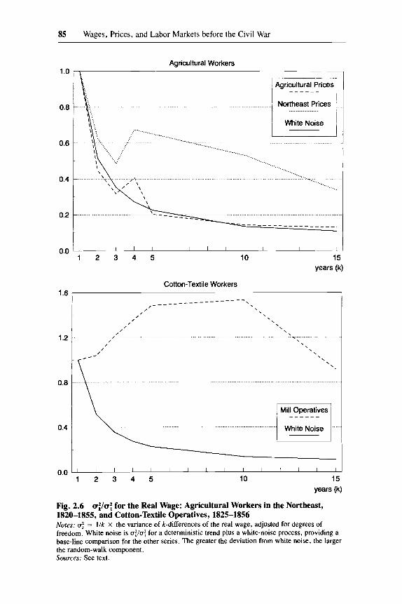
Further evidence on the persistence of shocks can be found in the upper panel of Figure 2.6, which analyzes real wages of agricultural workers in the Northeast, 1821-55, using data collected by Winifred R~thenberg .~’ We have deflated Rothenberg’s nominal wage series by our Northeast price index and by Rothenberg’s agricultural price index .32 Shocks to agricultural real wages appear to have been much less persistent than any of the series in Figure 2.5. Also in Figure 2.6, in the lower panel, are Cochrane tests on wages for cotton- mill operatives from Robert Layer’s study, which we have deflated by our Northeast price index. Nominal wages for cotton-mill operatives are virtually flat over the period, and, not surprisingly, real wages demonstrate extreme persistence of shocks.

We have also estimated persistence measures for industrial workers in the late nineteenth century, during 1870 to 1908 and the subperiod 1870 to 1897, but we emphasize the provisional nature of these results.?) We find that real wage data for the late nineteenth century demonstrate extreme persistence.

(2’) ( I - L)x, = k’ + A’(L)E,

where A’(L) = A(L)/B(L) and k’ = p /E(L) . Let A ’ ( ] ) = x a i , the infinite sum of the moving average coefficients of A ’ ( L ) . If x, is [(I), then A ’ ( L ) will converge to a finite and positive limit. This limit is the long-run “impulse-response” to a unit “innovation,” or shock in E,. See J. Camp- bell and G . Mankiw, “Are Output Fluctuations Transitory?’, Quarterly Journal of Economics, 102 (Nov. 1987), pp. 857-80. For example, if x, were a random walk with drift (x , = + x, , + E,). then A’ ( I ) = 1. Estimates of 8“; using the SAS PROC ARIMA procedure (available on request from Robert Margo) were less than one for all occupations in each region, which is consistent with the results of the Cochrane tests, which showed that the random-walk component of real wages was small.

31. See Winifred Rothenberg, “The Emergence of Farm Labor Markets and the Transformation of the Rural Economy: Massachusetts, 1750-1855,” Journal of Economic History, 48 (Sept. 1988), pp. 537-66.

32. When we deflate by Rothenberg’s agricultural price index (which she calls PI in “The Emergence of Farm Labor Markets”), the agricultural real wage (WWIIPI) is indistinguishable from a trend with white noise. Because our price index is heavily weighted toward agricultural commodities, the difference between the two indices seems curious. But Rothenberg apparently smoothed her price index with a three-year moving average (see Rothenberg, “The Market and Massachusetts Farmers,” p. 31 I ) , and that procedure could explain the differences in using her agricultural index.

33. We use the index of average daily wages in all industries (D 574) spliced at 1891 to (average weekly hours X average hourly earnings) for workers in manufacturing (D 593-94). The price index is the Warren and Pearson wholesale price index for all commodities (E 1) spliced at 1890 to the Bureau of Labor Statistics wholesale price index (E 13). All series are from Historical Statistics of the UnitedStates, Colonial Times to 1957 (Washington, D.C., 1960).


0.0 I 1 I I 1 I I 1 I 1 1 I 1 1

0.8

0.6

0.4

0.2

~-

Agricultural Prices _ _ _ _ _ _

. . . .

.................

..................................... . . . . . . . . . . . . . . . . .

1.6

1.2

0.8

0.4

0.0

1 2 3 4 5

Cotton-Textile Workers

10 15 years (k)

, , \

/ ,

/ ,

/ , \ t~ ........... .............. . . . . . . . . . . . . . . . . . . . . . . . . . . . . . . .

/ ------------------,

fi /

/ \

/ / ,

*- - , , \.

. . . . . . . . . . . . . . . . . . . . . . . . . . . . . . . . . . . . . . . . . .

I

Mill Operatives ------

I 1 I 1 I I I I I I I I I I

1 2 3 4 5 10 15 years (k)

Fig. 2.6 a:/a: for the Real Wage: Agricultural Workers in the Northeast, 1820-1855, and Cotton-Textile Operatives, 1825-1856 Notes: a; = I / k x the variance of k-differences of the real wage, adjusted for degrees of freedom. White noise is a:/u: for a deterministic trend plus a white-noise process, providing a base-line comparison for the other series. The greater the deviation from white noise, the larger the random-walk component. Sources: See text.


The period from 1870 to 1897 was one of secular deflation with one price spike during 1880 to 1885 and several smaller ones. Deflation, it appears, became a fact of economic life, and individuals adjusted their expectations accordingly. But gold discoveries in the mid-1 890s led to rapid and unantici- pated price increases, and expectations may have been slow to adjust. Thus the persistence of shocks to real wages during 1870 to 1897 appears much like that during the antebellum period. But the data including the post-1897 era distinctly do not. Shocks are as persistent as in a random-walk process for the first five years. Recent work using post-World War I1 data indicates that the persistence displayed by the 1870 to 1908 real wage series is characteristic of much of the twentieth century.34 Thus, in comparison with the later data, the antebellum series demonstrate considerably less persistence, and nominal wages appear more flexible in response to shocks.

Even though the random-walk component of antebellum real wages was small, it may have been the outcome of either persistent nominal or persistent real If long-run neutrality held, the random-walk component could only be the product of real Previous studies of long-run neutrality using late nineteenth and early twentieth century data provide mixed results. Although Joel Mokyr and Stephen DeCanio found no evidence against long- run neutrality for the 1861 to 1900 period, Jeffrey Sachs did in his regressions for the 1897 to 1929 period.37

We investigate long-run neutrality by examining the cointegration properties of wages, prices, and real GNP per worker.3s Speaking loosely, a collection of time series is cointegrated if the series are each integrated and the components do not drift arbitrarily apart from one another in the long run. The first condition, that concerning cointegration, holds if a linear combination of the series is stationary, even if the individual series are The first step is to estimate a “cointegrating” regression

34. See Kevin Hassett, “Persistence and Cyclicality in the Aggregate Labor Market” (manuscript, presented to the Labor Workshop, University of Pennsylvania, Nov. 1988).

35. By persistent nominal shocks we mean a violation of long-run neutrality. There is also the possibility that price fluctuations permanently altered real variables, which we do not investigate. Examples of real shocks are the introduction of the factory system, technological change, the opening of the Erie Canal, and high levels of immigration in the late 1840s and early 1850s.

36. In effect, the equilibrium path of real wages was not a deterministic trend, but a stochastic trend reflecting the impact of shocks to real variables determining labor supply and demand.

37. See Joel Mokyr and Stephen DeCanio, “Inflation and the Wage Lag During the American Civil War,” Explorarions in Economic History, 14 (Oct. 1977), pp. 31 1-36; and Jeffrey Sachs, “The Changing Cyclical Behavior of Wages and Prices: 1890-1 979,” American Economic Review, 70 (Mar. 1980), pp. 78-90. Sachs estimated regressions relating nominal wages to current prices, lagged prices, and GNP. He found the sum of the lagged price coefficients was less than unity, a result inconsistent with long-run neutrality.

38. See Robert F. Engle and C. W. 1. Granger, “Cointegration and Error-Correction: Represen- tation, Estimation, and Testing,” Econometrica, 55 (Mar. 1987), pp. 25 1-76, and Economerric Modelling Wirh Coinregrated Variables. special issue of the Oxford Bulletin of Economics and Statistics, 48 (Aug. 1986). for discussions of cointegration.

39. Unit root tests of real wages show that wages and prices do not cointegrate. A test of the Gallman-Berry output series (see below) also could not reject the hypothesis that the series pos- sesses a unit root.


for which all (lower-case) variables are in logs. The GNP variable is a combination of Robert Gallman’s and Thomas Senior Berry’s data for real gross national product in year t converted into a per-worker series. The Gallman- Berry index, as our spliced series will be called, is assumed to capture “real” factors determining the long-run equilibrium growth path of real wages.4o The “cointegrating vector” ( 1 - aI - a2) gives the long-run coefficients of the stationary linear c~ rnb ina t ion .~~

Separate regressions are estimated for each of the three occupations in the four regions using the annual series reported in Appendix A. Two test statistics are calculated from the estimated regression residuals: the cointegrating regression Durbin-Watson test statistic (CRDW) and the augmented Dickey- Fuller test statistic (ADF). The test for cointegration is, in effect, a test whether the regression residuals are ~ t a t iona ry .~~ As in the Dickey-Fuller test described earlier, the null hypothesis is that the three series are not cointegrated. The test results appear in Table 2.2. All of the CRDW statistics reject the null (accept cointegration) at the 5 percent level. The DF and ADF statistics are somewhat less conclusive, but still broadly support cointegration of wages, prices, and output per worker.

Interpreted literally, cointegration means that wages, prices, and per capita real output “moved together” in the long run. But the price coefficients in the cointegrating regressions (a, in Table 2.2) are substantially less than one, and those for clerks are negative in two cases, results that are inconsistent with long-run neutrality ( a I = 1). The price coefficients, however, are not robust to the estimating procedure. An equation regressing prices on wages, rather than the reverse, produces implied price coefficients that vary substantially and have ranges that include Because the R2’s for the cointegrating regressions are low, the al’s cannot be estimated with precision. We conclude that, while there is no evidence against long-run neutrality, there can be no definitive inference about the sources (nominal as opposed to real) of the random-walk component of real wages.

Having shown that wages, prices, and output per worker were cointegrated, our final step is to estimate “error-correction’’ regressions of nominal wages. Error correction refers to the notion that the coefficient 6, in equation (4), should be negative if the three series (wages, prices, and output per worker) were cointegrated. For example, if real wages were above their equilibrium value (a positive residual) in period ( t - l), then wages should fall in period 1.

40. Thomas Senior Berry, Production and Popularion since 1789: Revised GNP Series in Con- stant Dollars (Richmond, 1988); and Robert E. Gallman, unpublished data (June 1965). Annual labor force estimates for intercensal years were linearly interpolated from census benchmarks. Census estimates of the labor force are from Thomas Weiss, “Appendix: Estimation of the Ante- bellum Labor Force Figures” (manuscript, University of Kansas, May 1990), table A-I.

41. The cointegrating vector, however, need not be unique; see Engle and Granger, “Cointegra- tion and Error Correction.”

42. Ibid., p. 266, describe the various test statistics for cointegration. 43. If p is the coefficient on wages in the reverse regression, then a, = I@.


Table 2.2 Price Coefficients and Cointegration Tests of Wages, Prices, and Real GNP Per Capita, 1821-1856

Northeast Midwest South Atlantic South Central

Laborers “ I 0.060 0.350 0.239 0.140 CRDW 0.841* 1.555* 0.817* 0.943 DF - 2.872** -4.654* -2.237 - 3.130* ADF -3.421* - 2.438 -2.388 -3.263*

R2 0.434 0.465 0.141 0.258 Artisans

“1 0.247 0.486 0.164 0.221 CRDW 1.047* 0.974* 0.913* 0.902* DF -2.984** - 3.389* - 3.095** - 3.1 16** ADF - 2.246 - 3.188** - 2.825** - 3.863*

R2 0.454 0.473 0.322 6.171

“I -0.367 -0.121 0.190 -0.078 CRDW I .w* 0.843* 0.432* 0.601 * DF - 3.284** - 2.756 - 1.861 - 2.258 ADF -2.145 -2.012 -2.133 -2.956**

R2 0.679 0.703 0.221 0.478

Clerks

Notes: a, is the coefficient on the log of prices from the cointegrating regression, In W, = cto + “;In P, + “;In GNP, + p,.

CRDW is the Durbin-Watson statistic from the above cointegrating regression. DF is the t-statistic on 6 from the Dickey-Fuller regression

Ap = -8p_, + E.

ADF is the t-statistic on 6 from the augmented Dickey-Fuller regression, Ap = - 8 ~ _ ~ + P A F - ~ + o A ~ - ~ + E’.

The R,’s are those from the cointegrating regression. Critical values for CRDW, DF, and ADF statistics are from S. G. Hall, “An Application of the Granger and Engle Two-step Estimation Procedure to United Kingdom Aggregate Wage Data,” Oxford Bullerin of Economics and Statis- tics, 48 (Aug. 1986). p. 233. *Indicates the test accepts cointegration at the 5% level.

**Indicates the test accepts cointegration at the 10% level.

The estimates of 6 were, in fact, negative in all the regressions, and the majority were statistically significant. Because the sample sizes are small, the specification of the error-correction regressions is parsimonious:

(7) ( 1 - L)w = a(1 - L)p + p(1 - L)gnp + 6 e - , + E

where e - , is the lagged residual from the cointegrating regressions. The pur- pose of the regressions is to investigate the degree of contemporaneous re- sponsiveness of wages to nominal Ap and real Agnp shocks, that is, as re- vealed by the coefficients a and p.

Table 2.3 shows estimated values of a and p. Although few of the coefficients are statistically significant, the majority are positive in sign. For example, a positive productivity shock (Agnp > 0) generally caused nominal


Table 2.3 Error-Correction Regressions: Coefficients on the Change in the Log of Price (Ap) and the Change in the Log of GNP (Agnp)


Artisans P

gnP

Laborers P

Clerks P

0.310 (2.885)

-0.119 (0.641)

-0.039 (0.231) 0.095

(0.3 18)

-0.120 (0.736) 0.108

(0.376)

0. I27 (0.982) 0.290

(0.9 I 7)

0.094 (0.61 3) 0.258

(0.715)

-0.140 (0.922) 0.5 13

(1.349)

-0.017 (0.207) 0.096

(0.500)

0.305 (2.213) 0.242

(0.709)

0.238 (1.508)

-0.034 (0.093)

0.199 (1.589) 0.164

(0.6 19)

-0.017 (0.128) 0.367

(1.296)

0.039 (0.224)

(0.224) -0.084

Note: a and p are from regressions of the form given by equation (7): ( I -L)w =a( 1 -L )p + p( I -L)gnp + 6 e _ , + E

where e is the residual from the cointegrating regression; see Table 2.2. r-statistics are in paren- theses.

wages to increase in the same period. Antebellum wages were “procyclical” in this sense. Similarly, a positive price shock (Ap > 0) resulted in higher nominal wages. The estimates of a, however, are all substantially less than one, implying that contemporaneous changes in prices and real wages were negatively related. Thus, the persistence of shocks to real wages in the short run is largely attributable to the slowness with which nominal wages adjusted to changes in the price level.

2.4 Implications for Antebellum Labor Markets

Our various findings, by region and occupation, reveal much about the functioning of antebellum labor markets and the effects of economic development. To reiterate, our main finding is that although shocks to real wages across all regions and (nonagricultural) occupations had little long-run persistence, there was a substantial short-run impact. Agricultural real wages, however, display considerably less persistence. At the two extremes, the Mid- west and the South Atlantic were the most anomalous of the regions; the Mid- west having the least persistent, and the South Atlantic having the most persistent, shocks to real wages. Agricultural workers and clerks (also cotton- mill operatives) were at the two extremes of the occupations.

Why did shocks to real wages persist in the short run? Price fluctuations in the antebellum period were generally monetary in origin. The United States


was on a bimetallic standard but had no central bank to sterilize specie nor act as a “lender of the last resort” in times of banking crisis. Changes in specie, in the British discount rate, and in the cotton market led to sharp changes in the price level and often to banking panics.44

The precise mechanism underlying our results and causing monetary forces to have real effects may be related to Robert Lucas’s “signal processing” theory.45 A decrease in the money supply, for instance, is noticed by producers as a decrease in the price for their goods. But producers do not know whether the price change is general or relative, and they will attribute some of the change to each cause. Because they perceive that at least part of the decrease is specific to their industry or firm, they will decrease employment, invest- ment, and other real variables by some amount. They perceive that they cannot lower nominal wages by the full amount, because, if part of the change is relative, the decrease in wages would lead to an exodus of labor. Because all producers lay off some workers, a downturn ensues, and nominal wages eventually do fall. The absence of information, thus the noisiness of the signal, causes a purely monetary phenomenon to have real effects.

Rather than attributing the relationship between the monetary and real phenomena simply to nominal wage rigidity, Lucas’s signal processing theory is an equilibrium theory of adjustment in the face of imperfect information. Be- cause the theory is more believable when information is limited, it seems particularly relevant to the nineteenth century when the public was less knowl- edgeable about the course of general economic variables. Agents may have had more difficulty discerning absolute from relative price changes in indus- trialized areas producing a heterogeneous mix of products, such as the North- east, than in agricultural regions, such as the Midwest, where the product mix was more homogeneous. The lower persistence of shocks in the Midwest, especially among the unskilled, is also consistent with the view that a larger agricultural sector contributed to more flexible labor markets for free workers. The more persistent shocks in the Old South, however, appear to contradict claims that slavery enhanced the spatial efficiency of free labor markets, thereby inhibiting industrial development in the region.46

44. See, for example, Temin, The Jacksonian Economy. Recent work on financial crises suggests that antebellum banking panics could have had persistent effects on real wages. Disruptions in the credit mechanism resulting in credit rationing might have reduced the demand for labor, causing a reduction in real wages. On the real effects of financial crises, see Ben S. Bernanke, “Nonmonetary Effects of the Financial Crisis in the Propagation of the Great Depression,” Amer- ican Economic Review, 73 (June 1983), pp. 257-76.

45. See, for example, Robert Lucas, Studies in Business-Cycle Theory (Cambridge, Mass., 1981), in particular the reprinted article, “Expectations and the Neutrality of Money,” and the essay “Understanding Business Cycles.”

46. See Heywood Fleisig, “Slavery, the Supply of Agricultural Labor, and the Industrialization of the South,”Journal ofEconomic History, 36 (Sept. 1976), pp. 572-97. Recent work by Gavin Wright suggests that inefficient labor markets may have inhibited southern economic growth after the Civil War; our results suggest that inefficiencies existed during the antebellum period as well; see Gavin Wright, Old South, New South (New York, 1986).


There is, however, a competing explanation for the behavior of midwestern wages. Land sales in the Midwest (and South Central regions) skyrocketed during the price inflation of the 1830s. In both regions land sales at the peak of the land boom, in 1836, were eight times their 1830 The land boom, according to some, developed because land prices were fixed in nominal terms while output prices, especially cotton, were rapidly rising. Land, therefore, became an exceptional bargain.4R Fluctuations in land sales appear strikingly similar to those of prices, although land sales are considerably more extreme. The demand for labor, particularly unskilled labor, may have increased with the land boom, thereby producing greater flexibility of wages in the The relationship between prices and nominal wages, therefore, may have been intermediated by a third factor-land. This explanation is ap- pealing, but is not entirely consistent with the evidence. Real wages did not always increase during the land boom period; further, nominal wages in the South Central region, which also experienced a spectacular land boom, do not yield the same results.

We turn now to the implications of our findings for the functioning of labor markets. Most laborers in the antebellum period were paid by the day or the month and did not, it seems, have the explicit or implicit guarantees workers have today. Rigid nominal wages in the face of declining prices might then imply high levels of unemployment. If workers were relatively immobile, unemployment could have meant prolonged absence of work and wages. Given the signal processing model just sketched, price decreases, even if triggered by purely monetary phenomena, could have produced unemployment, economic depression, and, paradoxically, rising real wages for those who re- mained employed. Real wages did, in fact, rise during most episodes charac- terized by labor historians and others as ones of major unemployment, for example, 1839-42 and 1854-55.50

There is some evidence that workers laid off during periods of economic decline migrated to agricultural areas and later returned to their original employment when conditions impr~ved .~ ’ Thus unemployment in the industrial

47. See the appendix in Stanley Lebergott, “The Demand for Land: The United States, 1820- 1860,” Journal of Economic History, 45 (June 1989, pp. 181-212.

48. See, for example, Temin, The Jacksonian Economy. It should also be noted that land became easier to purchase after 1832, when an act was passed which reduced the minimum acreage.

49. Because the price index does not include the cost of housing (which would have risen during the land boom), it is also possible that our real wage index overstates the flexibility of midwestern wages.

50. Layer, Earnings of Cotton Mill Operatives, notes employment was reduced during 1834, 1837, 1842, 1850, 1856. The episodes given are from Wilentz, ChantsDemocratic.

5 I . Alan Dawley, in Class and Community: The Industrial Revolution in Lynn (Cambridge, Mass., 1976), writes that “manufacturers . . . hired a large number of people to get the job done, and then laid off most of the employees when the orders were filled. . . . When the shoe industry expanded, new job opportunities attracted migrants to the city, and when it retrenched the inflow stopped. The boom of the 1830s came to an abrupt halt in 1837; for the next several years Lynn experienced an outright decline in population; then business revival in the mid-1 840s brought renewed population growth” (p. 53).


sector may have been less severe than various historical accounts suggest. But migration from urban and industrial areas could have exacerbated the adjustment by preventing firms from observing the signal of general unemployment.

Price inflation, by similar reasoning, produced decreased real earnings and an increased demand for labor. Historically, labor unrest and strikes in the Northeast are easily linked to these episodes; important strikes occurred in virtually all the inflationary periods, for example, 1824-25, 1835-36, 1844- 45, and 1853-54. According to the standard count of strikes between 1833 and 1837, when the price level rose sharply, the vast majority involved skilled workers in the Northeast; very few took place among the unskilled or in other regions.52 Although striking for higher wages was not “the journeyman’s sole or even major concern,” there is no question that labor agitation was “clearly linked to the inflationary spiral.”53 Although persistence of shocks was somewhat diminished for northeastern artisans, compared with those in other regions, collective action did not greatly reduce it.

The persistence of shocks to clerks’ wages is consistent with their relatively high degree of skill and the nature of white-collar work during the period. Often employed for long period of time at the same firm, there was less need for white-collar workers to resort to strikes and union activity, since real wage losses during inflationary periods would be balanced by gains during defla- tionary episodes.

Economic historians have long debated whether the existence of a wage lag helped finance the Union war effort during the Civil War.54 An econometric study by Mokyr and DeCanio, using methods different from ours, concluded that a wage lag did exist during the Civil War, but they did not consider whether the lag was peculiar to the war period.55 Our results suggest that the wage lag may have been a pervasive feature of American labor markets long before the Civil War and that it increased over time.

2.5 Summary

We have presented an econometric analysis of the persistence of shocks to real wages before the Civil War. The results suggest that the revisionist de- scription of antebellum labor markets has merit. We found no evidence against the view that changes in prices were eventually reflected fully in nom-

52. Commons, et al., History of Labor, vol. I , pp. 478-84 contains the list of strikes between I833 and 1837. 53. Wilentz, Chanrs Democratic, p. 231. Wilentz also notes that a strike by journeyman cabi-

netmakers in 1835 was motivated by the fact that “the price book [for standard journeyman wages] used by their masters was more than a quarter of a century old. . . . The old book failed to keep up with the cost of living” (p. 232). 54. The wage-lag hypothesis was first articulated by Wesley Clair Mitchell, A History of the

Greenbacks (Chicago, 1903). Mitchell’s hypothesis was criticized by, among others, R. A. Kessel and A. A. Alchian, “Real Wages in the North During the Civil War: Mitchell’s Data Reinter- preted,” Journal ofLaw and Economics, 2 (Oct. 1959), pp. 95-1 13. 55. Mokyr and DeCanio, “Inflation and the Wage Lag During the American Civil War.”


inal wages, controlling for real factors. In the short run, however, shocks to real wages had persistent effects. Real wages generally fell during periods of inflation and rose during periods of deflation. Antebellum deflations went hand in hand with recession or depression, and almost all involved episodes of reduced employment in industry and urban areas. Only fully employed workers, therefore, benefited from real wage growth during deflations. 0th- ers, it seems, were either out of work or migrated to agriculture. The emphasis labor historians have given to the wage lag in explaining labor strife, and in accounting for the importance of inconstant employment in working class culture and politics, seems deserved. But the flexibility of the antebellum labor force and the role of the agricultural hinterland in shielding labor from unemployment requires further investigation.

Appendix A

Table 2A.1 Indices of Nominal Wages of Artisans, 1820-1856 ~ ~

Year Northeast Midwest South Atlantic South Central

1820 1821 1822 1823 1824 I825 1826 1827 1828 1829 1830 1831 1832 1833 1834 1835 1836 1837 1838 1839 1840 1841 1842 1843 1844 1845 1846 1847 1848 1849 1850 1851 1852 1853 1854 1855 1856

79.4 56.3 71.2 70.4 70.4 67.7 64.9 74.3 68.9 65.7 62.9 66.4 68.9 67.8 76.6 78.9 84.5 80.3 77.6 82.5 77.6 77.6 70.8 75.4 67.0 80.0 76.9 78.4 74.0 74.6 75.1 74.1 76.8 79.5 84.7 89.9

100.0

Decadal averages (1821-30 = 100): 1821-30 100.0 1831-40 113.1 184140 111.5 1851-56 125.2

Rate of growth’ 0.8

n.a. n.a. 69.7 69.2 69.2 68.7 68.2 73.9 79.6 85.3 85.9 97.5 93.8 88.2 86.8 85.5 84.2

114.3 92.8 83.9 84.7 79.5 73.6 61.8 65.7 69.8 60.1 68.9 72.9 76.0 79.0 89.6 87.5 93.6 94.8 98.1

100.0

100.0 122.6 95.0

126.2

0.8

n.a. n.a. n.a. 82.6 79.0 87.4 95.8 99.0 88.5 93.6 95.0 96.4 95.8 95.8 97.5 98.6 90.9 92.1 93.3 93.3 93.0 92.6 95.5 84.0 84.0 84.6 84.6 83.0 86.0 87.6 89.1 89.1 96.2

103.3 110.4 117.5 100.0

100.0 105. I 96.1

114.1

0.5

80.2 84.0 87.7 95.9 94.3 99.2

104.2 109.2 104.4 90.0 95.0 93.4 91.8 97.3

102.8 108.0 115.8 108.8 90.2

110.6 117.6 124.5 111.2 87.9 84.6 96.5 88.0 99.2 93.3

101.4 109.4 110.0 110.0 109.4 106.5 108.5 100.0

100.0 107.5 103.3 111.4

0.4

Notes: See also Appendix B for a procedure to convert the wage indices to wage levels. Source; Margo-Villaflor sample of “Reports and Articles Hired,” National Archives, Record Group 92. n.a. = not available. ”Rate of growth is the average annual rate of growth, 1821-30 to 1851-56.


Table 2A.2


Indices of Nominal Wages of Laborers, 1820-1856

1820 1821

1823 1824 1825 1826 1827 1828 1829 1830 1831 1832 1833 1834 1835 1836 1837 1838 1839 1840 1841 1842 1843 1844 1845 1846 1847 1848 1849 1850 1851 1852 1853 1854 1855 1856

1822

n.a. 66.4 64.1 64.1 63.8 69.7 75.5 71.5 64.3 60.7 61.1 60.2 63.2 62.4 74.7 74.7 81.8 88.2 80.1 71.5 59.0 73.1 74.4 81.5 81.5 81.5 83.4 69.4 76.7 84.0 85.3 80.7 89.0 88.1 92.4 95.5

100.0

Decadal averages (1821-30 = 100): 1821-30 100.0 183140 108.3 184140 119.5 1851-56 137.6

Rate of growth” 1.1

84.5 86.3 70.5 67.1 65.5 65.2 63.8 63.8 68.2 71.1 73.8 69.8 73.8 83.6 93.3 93.3 78.0

117.4 88.6

107.4 85.1 80.8 76.4 82.7 80.0 77.3 88.9 73.9 90.8 86.6 82.4 87.0 91.5 87.8

100.5 105.2 100.0

100.0 128.5 118.0 137.1

1 . 1

n.a. n.a. n.a. n.a. n.a. 74.8 76.8 77.8 79.4 74.9 70.4 68.5 66.6 65.2 63.8 67.6 84.3 87.6 74.3 81.1 79.8 78.4 60.6 72.3 74.3 76.3 77.3 77.5 75.9 74.0 72.1 71.2 70.3 70.3 71.2 89.4

100.0

100.0 97.6 97.6

104.0

0.1

73.9 79.9 79.9 80.9 79.9 77.8 77.0 84.3 91.6 96.0 97.7 90.8 90.3 88.6 92.4 83.8 99.8

102.3 76.7 95.7 90.8

101.1 99.1 92.7 92.9 83.1 73.3 72.4 78.6 84.9 91.1 96.8

108.0 105.7 100.9 105.0 100.0

100.0 107.8 103.4 121.5

0.7

Notes: See also Appendix B for a procedure to convert the wage indices to wage levels. Source: Margo-Villaflor sample of “Reports and Articles Hired,” National Archives, Record Group 92. n.a. = not available. ‘Rate of growth is the average annual rate of growth, 1821-30 to 1851-56.


Table 2A.3 Indices of Nominal Wages of Clerks, 1820-1856


1820 1821 1822 I823 1824 I825 1826 1827 1828 1829 1830 1831 1832 1833 I834 1835 1836 1837 1838 1839 1840 1841 1842 I843 1844 1845 I846 1847 1848 1849 I850 1851 1852 1853 1854 1855 1856

89.9 83.2 59.3 62.9 62.8 65.6 60.7 6.5.6 70.3 78.8 64.2 73.6 72.2 71.1 71.1 71.1 71.0 82.0 74.8 87.8 87.8 84.5 84. I 94.7 99.5 99.5 93.7 94.4

105.3 107.6 109.9 103.3 96.9 95.1

114.1 108.6 100.0

Deradal averages (1821-30= 100): 182 1-30 100.0 183140 113.4 184140 144.6 1851-56 153.0

Rate of growth” 1 .5

49.7 55.8 46.8 45.9 45.1 49.9 49.9 45.7 48.3 48.9 49.9 43.0 50. 1 50.2 56.0 49.5 50.5 55.9 58.2 60.1 55.0 54.0 58.6 69. I 67.3 69.1 62.5 69.6 92.7 85.0 77.3 71.0 88.1 71.1 78.9 88.3

100.0

100.0 108.8 145. I 170.5

1.9

n.a. n.a. n.a. 88.9 98.5 87.3 77.6 77.3 86.3 69.9 65.9 61.8 63.9 72.0 80. I 76.5 93.5 99.2

104.0 106.6 94.4

103.6 92.3 76.1 78.9 81.7 84.5 99.0

113.5 116.5 119.4 112.4 109.9 107.6 95.0

100.0 108.9

100.0 104.5 118.5 129.6

0.9

n.a. 71.0 77.3 53.0 55.5 62.0 68.4 68.1 73.5 78.9 79.4 78.7 76.0 74.1 72. I 78.1 79. I 96.2

104.3 125.1 114.6 104.1 93.2 87.3 89.4 91.5

109.6 111.4 113.1 108.5 103.9 109.5 105.5 110.3 122.1 103.7 100.0

100.0 130.7 147.3 157.9

1.6

Notes: See also Appendix B for a procedure to convert the wage indices to wage levels. Source: Margo-Villaflor sample of “Reports and Articles Hired,” National Archives, Record Group 92. n.a. = not available. “Rate of growth i s the average annual rate of growth, 1821-30 to 1851-56.


Table 2A.4 mice Indices, 1821-1856


1821 1822 1823 I824 1825 1826 I827 1828 1829 I830 1831 1832 1833 1834 1835 1836 I837 I838 1839 1840 1841 1842 1843 1844 1845 1846 1847 1848 1849 1850 1851 I852 I853 1854 1855 1856

98.6 103.0 95.5 93.0 95.8 86.5 85.3 83.1 80.8 78.9 81.4 85.0 90.1 84.6 96.4

110.2 103.7 98.7

103.9 85.0 78.8 68.3 62.2 61.1 68.2 68.5 82.9 69.7 72.3 78.0 74.7 78.8 86.4 93.8 96.8

100.0

Decadal averages (1821-30 = 100): 182 1-30 100.0 183 1 4 0 104.2 184140 78.8 1851-56 98.0

Rare of growth” - 0.07

80.6 86.6 74.1 72.2 74.4 63.1 62.8 64.5 73.7 67.9 68.7 74.2 77.8 74.8 90.0

106.5 100.2 92.0 96.8 73. I 65.3 51.3 53.6 58.7 61.5 63.5 77.4 59.6 65.4 12.7 73.1 16.9 81.3 84.5 96.3

100.0

100.0 118.6 87.4

118.6

0.6

100. I 109.5 101.6 94.4 96.6 86.3 86.1 82.8 81.1 83.1 79.0 83.5 89.2 91 .O

102.1 127.5 111.7 105.5 108.1 83.6 80.3 61.3 60.3 62.8 68.9 73.4 85.4 64.5 71.6 80.9 83.3 83.3 87.0 88.8

101.1 100.0

100.0 106.5 77.0 98.4

- 0.06

100.3 113.6 102.2 95.8

104.1 92.8 89.9 93.3 91.6 83.4 85.4 89.8 92.9 89.9

106.0 128.5 116.9 115.9 110.4 91.5 88.4 77.0 62.7 65.6 67.3 68.8 85.6 68.7 75.2 85.8 79.0 79.1 85.1 85.6

100. 1 100.0

100.0 106.2 77.0 91.2

-0.3

Source; See Appendix B and text. ’Rate of growth is the average annual rate of growth, 1821-30 to 1851-56.


Table 2A.5


Indices of Real Wages of Artisans, 1821-1856

1821 1822 1823 1824 1825 1826 1827 1828 1829 1830 1831 1832 1833 1834 1835 1836 1837 1838 1839 1840 1841 1842 I843 1844 1845 1846 1847 1848 1849 1850 1851 1852 1853 1854 1855 1856

57.1 69.1 73.7 75.7 70.7 75.0 87.1 82.9 81.3 79.7 81.6 81.1 75.2 90.5 81.8 76.7 77.4 78.6 79.4 91.3 98.5

103.7 121.2 109.7 117.3 112.3 94.6

106.2 103.2 96.3 99.2 97.5 92.0 90.3 92.9

100.0

Decadal averages (1821-30= 100): 1821-30 100.0 183140 108.2 184140 141.2 1851-56 126.7

Rate of growth' 0.8

n.a. 80.5 93.4 95.8 92.3

107.1 117.1 123.4 115.7 126.5 141.9 126.4 113.3 116.0 95.0 79.1

114.1 100.9 86.7

115.9 121.7 143.5 115.3 111.9 113.5 94.6 89.0

122.3 116.2 108.7 122.6 113.8 115.1 112.2 101.9 100.0

100.0 102.9 107.5 104.8

0.2

n.a. n.a. 81.3 83.6 90.5

110.0 115.0 106.8 115.4 114.3 122.0 114.7 107.3 107.1 96.6 71.3 82.5 88.4 86.3

111.2 115.3 155.8 139.3 133.8 122.8 115.3 97.2

133.3 122.3 110.1 106.9 115.5 118.7 124.3 116.2 100.0

100.0 96.7

121.9 111.3

0.4

83.7 77.2 93.8 98.4 95.3

112.3 121.5 111.9 98.3

113.9 109.4 102.2 104.7 114.3 101.9 90.1 93.1 77.8

100.2 128.5 140.8 144.4 140.2 129.0 143.4 127.9 115.9 135.8 134.8 127.5 139.2 139.1 128.6 124.4 108.4 100.0

100.0 101.5 133.2 122.6

0.7

Sources: Tables 2A.1 and 2A.4. n.a. = not available. "ate of growth is the average annual rate of growth, 1821-30 to 1851-56.


Table 2A.6 Indices of Real Wages of Laborers, 1821-1856 ~~


1821 1822 1823 1824 1825 1826 1827 1828 1829 1830 1831 1832 1833 I834 1835 1836 1837 1838 1839 1840 1841 1842 1843 1844 1845 1846 1847 1848 1849 1850 1851 1852 1853 1854 1855 1856

67.3 62.2 67.1 68.6 72.8 87.3 83.8 77.4 75.1 77.4 74.0 74.4 69.3 88.3 77.5 74.2 85.1 81.2 68.8 69.4 92.8

108.9 131.0 133.4 119.5 121.8 83.7

110.0 116.2 109.4 108.0 112.9 102.0 98.5 98.7

100.0

Decadal averages (1821-30 = 100): 1821-30 100.0 183140 103.1 184140 152.5 1851-56 139.9

Rate of growth' 1.2

107.1 81.4 90.6 90.7 87.6

100.2 101.6 105.7 96.4

108.7 101.6 99.5

107.5 124.7 103.7 73.2

117.2 96.3

111.0 116.4 123.7 148.9 154.3 136.2 125.7 140.0 95.5

152.3 132.4 113.3 119.0 119.0 108.0 118.9 109.2 100.0

100.0 108.4 136.3 115.9

0.5

n.a. n.a. n.a. n.a. 77.4 89.9 90.4 95.9 92.4 84.7 86.7 79.8 73.1 70.1 66.2 66.1 78.4 70.4 75.0 95.5 97.6 98.9

119.9 118.3 110.7 105.3 90.7

117.7 103.4 89.4 85.5 84.4 80.8 80.2 88.4

100.0

100.0 86.0

118.9 97.9

-0.08

79.7 70.3 79.2 83.4 74.7 82.9 93.8 98.2

104.8 117.1 106.3 100.6 95.4

102.8 79.1 77.7 87.5 66.2 86.7 99.2

114.4 128.7 147.8 141.6 123.5 106.5 84.6

114.4 112.9 106.2 122.5 136.5 124.2 117.9 104.9 100.0

100.0 102.0 133.6 133.1

1 .o

Sources: Tables 2A.2 and 2A.4. n.a. = not available. 'Rate of growth is the average annual rate of growth, 1821-30 to 1851-56.


Table 2A.7 Indices of Real Wages of Clerks, 1821-1856


1821 1822 1823 1824 1825 1826 1827 1828 1829 1830 1831 1832 1833 1834 1835 1836 1837 1838 1839 I840 1841 I842 1843 1844 1845 1846 1847 1848 1849 1850 1851 1852 1853 1854 1855 1856

84.4 57.5 65.9 67.5 68.5 70.1 76.9 84.6 97.5 81.3 90.4 84.9 78.9 84.0 73.7 64.5 79.1 75.7 84.5

103.3 107.3 123.1 152.3 162.8 145.9 136.8 113.9 151.1 148.9 140.9 138.4 122.9 110.1 121.6 112.2 100.0

Decadal averages (1821-30= 100): 1821-30 100.0 183140 108.6 184 1-40. 183.4 1851-56 155.8

Rate of growtha 1.6

69.2 54.0 61.9 62.5 67.1 78.3 72.8 74.9 66.4 73.5 62.6 67.5 64.5 74.9 55.0 47.4 55.8 63.2 62. I 75.2 82.7

114.2 128.9 114.7 112.4 98.4 89.9

155.5 129.9 106.3 97.1

114.6 87.5 93.3 91.7

100.0

100.0 92.2

166.3 143.0

1.3

n.a. n.a. 87.0

102.8 94.1 83.6 86.0 92.5 76.3 79.0 72.4 71.2 77.5 89.1 72.2 72.8 84.9 89.7 96.6

103.7 117.2 119.9 121.4 120.3 121.4 122.8 115.7 165.2 154.9 139.2 141.9 138.9 126.4 111.0 108.8 100.0

100.0 93.5

148.0 138.2

1.2

70.8 68.0 51.9 57.9 59.6 73.7 75.8 78.8 86. I 95.2 92.2 84.6 79.8 80.2 73.7 61.6 82.3 90.0

113.3 125.2 117.8 121.0 139.2 132.8 136.0 159.3 130.1 164.6 144.3 121.1 138.6 133.4 129.6 142.6 103.6 100.0

100.0 123.0 190.3 173.5

2.0

Sources: Tables 2A.3 and 2A.4. *Rate of growth is the average annual rate of growth, 1821-30 to 1851-56


Appendix B Construction of the Wage and Regional Price Indices

Wage Indices

The nominal wage indices in Tables 2A.1-2A.3 are constructed so that 1856 = 100, and therefore cannot be used to compute skill differentials or ratios. The following are a set of nominal wages for 1856 that can be used to produce nominal wages for all years.


Artisans 1.91 2.21 1.74 1.91 Laborers 1.26 1.36 1.02 1.22 Clerks 2.14 2.21 2.35 2.52

Nores: Artisans includes carpenters, painters and plasterers, blacksmiths and machinists. Labor- ers includes common laborers and teamsters. Clerks includes inspectors and foragers.

Because the wages analyzed here havz been computed using a hedonic regression, those given above for 1856 depend on the weights placed on the coefficients. The procedure used is as follows. The coefficients from the hedonic wage regression for the fort and occupation dummies were weighted by the sample shares (e.g., the coefficient of the fort dummy for Detroit in the Mid- west laborer regression was weighted by the share of observations from De- troit). Coefficients of the seasonal dummies were each weighted by %I, and all other variables were set equal to zero. The estimates, therefore, can be interpreted as the daily wage (without rations) in the particular occupational group in 1856 averaged across forts in the region and across seasons.

To produce similar estimates for other years, multiply the wage estimate for 1856 by the index numbers reported in the appendix tables and divide by 100. For example, the index number for clerks in the Northeast in 1840 is 87.8. Thus the estimated clerks’ wage at Northeast forts in 1840 is $1.88 ( = $2.14 x 0.878). We emphasize, however, that wage estimates for artisans and laborers produced in this manner are not comparable to those in Robert A. Margo and Georgia C. Villaflor, “The Growth of Wages in Antebellum Amer- ica: New Evidence,” Journal of Economic History, 47 (Dec. 1987), pp. 873- 95, because they were produced using a different weighting procedure than that just described.

Price Indices

For each census region a set of commodities was selected from Arthur H. Cole’s compendium of price data. Average annual prices were calculated, and commodity-specific indices were formed (base year is 1856) in the usual manner. The regional price indices are geometric weighted averages of the commodity-specific indices:56

56. See Cole, Wholesale Prices. Although geometric weighted-average price indices are theo- retically inferior to other functional forms, the information required to calculate more complicated


P = rI,p,;(I)

where pi, is the value of the commodity-specific index in year t , and the s(i)’s are weights. The weights are analogous to budget shares and are derived from Ethel Hoover’s study of consumer prices.s7 Using the Carroll Wright sample of Massachusetts families, Hoover divided household expenditures into nine categories. For six of these categories (cereal and bakery products, meat and fish, dairy, other foods, clothing, and fuel), prices could be found in the Cole collection for commodities within each category. The Cole collection also contains price quotations for a tenth group, liquor, which Hoover did not include in her consumer price index.58 commodity-specific indices were then calculated and weights assigned to each index depending on the relative budget shares within categories.

To take a specific example, consider the category “cereal and bakery products’’ for the Northeast. The Cole collection contains prices for three commodities within this group-flour, cornmeal, and rice-for New York and Phila- delphia. According to Hoover’s calculations, flour accounted for 88 percent of all cereal and bakery expenditures on flour, cornmeal, and rice; the other relative shares are: cornmeal (0. lo), rice (0.02). Cereal and bakery products, according to Hoover, made up 10.8 percent of all household expenditures, and expenditures on the seven groups represented were 70.7 percent of all household expenditures. Thus the Northeast weight for flour (see below) is 0.134 (0.88 X 0.108/0.707). The remaining weights, listed below, were derived in a similar manner.

It is important to note that the South Atlantic index is the least satisfactory. The Cole collection contains no usable data for fuel prices for Charleston (either coal or wood) covering the entire period. Furthermore, the “meats and fish” and “clothing” categories cover only a single commodity each (bacon and cotton, respectively). If prices for these commodities evolved in a different way than for the other commodities in the category, the regional index may be biased. Investigating such biases would require the collection of additional price data, which is beyond our scope here.

indices is not available. Furthermore, a geometric index would appear to be more consonant with consumer theory than, for example, an algebraic weighted-average. Specifically, the geometric average is consistent with a Cobb-Douglas utility function, while an algebraic index is inconsistent with utility maximization. On price indices in general see W. E. Diewert, “Index Numbers,” in J. Eatwell, M. Milgate, and P. Newman, eds., The New Palgrave: A Dictionary ofEconomics, vol. 2 (New York, 1987), pp. 767-80.

57. Ethel D. Hoover, “Retail Prices After 1850,” in Conference on Research in Income and Wealth, vol. 24, Trends in the American Economy in the Nineteenrh Century (Princeton, 1960). pp. 177-78.

58. The budget share for liquor (0.02 of total consumer expenditures) is assumed to be the same for all regions and is derived from regressions in Michael Haines, “Consumer Behavior and Im- migrant Assimilation: A Comparison of the United States, Britain, and Germany, 188911 890’ (manuscript, Department of Economics, Wayne State University, Jan. 1988).


1. Northeast, commodities and weights: 1.1 Cereal and bakery products: flour (0.134), cornmeal (0.015),

rice (0.003) 1.2 Meats and fish: beef (0.113), pork (0.024), bacon (0.026),

fish (0.024) 1.3 Dairy: butter (0.130) 1.4 Other foods: molasses (0.003), coffee (0.067), tea (0.022),

1.5 Clothing: cotton (0.156), leather (0.054) 1.6 Fuel: coal (0.098) 1.7 Liquor: whiskey (0.028)

Percent of household expenditure accounted for by above commodities

lard (0.025), sugar (0.075)

= 70.7%59

2 . Midwest, commodities and weights: 2.1 Cereal and bakery products:

2.2 Meats and fish: pork (0.087), bacon (0.102) 2.3 Dairy: butter (0.130) 2.4 Other foods: coffee (0.075), sugar (0.085), lard (0.029),

2.5 Clothing: cotton (0.156), leather (0.054) 2.6 Fuel: coal (0.098) 2.7 Liquor: whiskey (0.028)


flour (0.150), rice (0.003).

molasses (0.004)

= 70.7%

3. South Atlantic, commodities and weights: 3.1 Cereal and bakery products: flour (0.167), rice (0.003) 3.2 Meats and fish: bacon (0.209) 3.3 Dairy: butter (0.144) 3.4 Other foods: coffee (0.083), lard (0.032), sugar (0.094),

3.5 Clothing: cotton (0.233) 3.6 Liquor: (0.031)

Percent of household expenditure accounted for by above commodities = 65.1%

molasses (0.004)

59. Of the expenditures of a typical antebellum household, 70.7 percent were on the listed commodities, in all but the South Atlantic region. The major excluded commodity is housing, for which there is no information in Cole’s collection. For the South Atlantic, the commodities included account for slightly less of total expenditure.


4 . South Central, commodities and weights: 4.1 4.2

fish (0.024) 4.3 Dairy: butter (0.130) 4.4 Other foods: coffee (0.067), tea (0.022), sugar (0.075),

4.5 Clothing: cotton (0.21 1) 4.6 Fuel: wood (0.098) 4.7 Liquor: whiskey (0.028)


Cereal and bakery products: flour (0.150), rice (0.003) Meats and fish: beef (0.113), pork (0.024), bacon (0.026),

lard (0.025), molasses (0.003)

= 70.7%

Documents

Wages, Prices, and Labor Markets before the Civil War Wages, Prices, and Labor Markets before the Civil War Claudia Goldin and Robert A. Margo 2.1 Economic Development, Nominal Wage