Embed Size (px)
Citation preview

Wages, Human Capital, and the Allocation
of Labor across Sectors∗
Berthold Herrendorf and Todd Schoellman†
March 6, 2014
Abstract
We document for nine countries ranging from rich (Canada, U.S.) to poor (India,
Indonesia) that average wages are higher in non–agriculture than in agriculture. We
measure sectoral human capital and find that it accounts for the entire wage gap in
the U.S. and most of the wage gaps elsewhere. We develop a multi–sector model that
explains these finding if: (i) Mincer returns to schooling are equal in both sectors;
(ii) more able workers sort into non–agriculture; (iii) distortions to the allocation of
labor between sectors are negligible in the U.S. and small elsewhere.
∗We would like to thank Gustavo Ventura for many helpful discussions. Herrendorf thanks the SpanishMinistry of Education for research support (Grant ECO2012–31358) and the University of Mannheim forits hospitality during a sabbatical when this project originated. The usual disclaimer applies.†Address: Department of Economics, W.P. Carey School of Business, Arizona State University, Tempe,
AZ 85287–9801, USA. E-mails: [email protected] and [email protected]

1 Introduction
In his Nobel prize lecture, Kuznets (1973) included the process of structural transformation,
that is, the reallocation of labor into other sectors of the economy, as one of the six main
features of modern economic growth. Nonetheless there are two rather different views
of structural transformation within the macro–development literature. One strand of the
literature assumes that at each moment labor is allocated efficiently between sectors and
derives the properties of preferences and technological progress that generate structural
transformation as a consequence of growth; see e.g. Herrendorf, Rogerson and Valentinyi
(2013) and the references therein. In contrast, a second strand of the literature measures
large gaps in labor productivity between agriculture and the rest of the economy. Since it
is difficult to account for these gaps, this strand of the literature concludes that labor must
be allocated inefficiently between sectors, with the reallocation of labor in poor countries
hindered by what is typically referred to as barriers or wedges; see e.g. Caselli (2005) and
Restuccia, Yang and Zhu (2008). According to this logic, the removal of barriers would
allow labor to move out of agriculture and would generate growth. This is precisely the
opposite direction of causality as in the first strand of the literature. It follows that given
the same stylized fact these two strands of the macro–development literature will make
vastly different policy prescriptions.
Somewhat surprisingly, there is little hard evidence on whether or not the allocation of
labor between non–agriculture and agriculture is efficient. The contribution of this paper is
to provide such evidence for multiple years and nine countries ranging from rich (Canada,
U.S.) to poor (India, Indonesia). The selection criterion for our countries is access to
sufficiently detailed data that allow us to calculate wages and construct human capital
at the sectoral level. For the U.S. these data are from the CPS, the Census, and the
American Community Survey (ACS) and they cover the period 1980–2011. For the other
eight countries, these data are from 26 population censuses that are harmonized by IPUMS
and range from 1970 to 2010. We document that there are large gaps between the average
wages per worker in non–agriculture and agriculture in all countries including the U.S.
We decompose the wage gaps into differences in the observable characteristics of workers;
differences in the returns to observable characteristics; residual wage gaps.
For the U.S., we find that the wage gaps are entirely accounted for by differences in
observables: non–agricultural workers have more years of schooling and earn higher Min-
cer returns to schooling than agricultural workers. There two different interpretations of
this finding. The “sectoral view” attributes the differences in Mincer returns to sectoral
1

technologies: schooling generates less human capital for workers who choose agriculture.
The “selection view” attributes the differences to the workers: schooling generates the
same human capital in each sector, but workers sort according to their unobserved ability.
Both views have the potential to explain why non–agriculture has more human capital and
higher Mincer returns than agriculture. To help us distinguish between them, we construct
a multi–sector model in which workers choose in which sector they work. We assume that
workers differ in their unobserved innate ability and their years of schooling and that sectors
potentially differ in the technology that translates these characteristics into human capital.
We also allow for the possibility of distorting barriers/wedges. We show that to account for
the U.S. findings we need to restrict our model along two dimensions: (i) both sectors have
the same technology; (ii) there are no barriers/wedges to the allocation of labor. Note that
(i) implies that a given worker gets the same returns to his characteristics in both sectors,
which of course is the selection view. Under these restrictions, our model has a sorting
equilibrium with the following properties: workers in non–agriculture have more years of
schooling, higher innate ability, and more human capital; average wages per worker are
higher in non–agriculture; average wages per efficiency unit are equalized between the two
sectors. The restriction that both sectors have the same technology has the testable impli-
cation that individuals who switch between sectors should not experience sizeable changes
in the returns to their observable characteristics. We provide evidence from the CPS that
is broadly consistent with that view.
For the other countries, we find that most of the wage gaps are accounted for by dif-
ferences in observables: non–agricultural workers once again have more years of schooling
and earn higher Mincer returns on schooling; differences in the residual wage gap are small
in comparison to the differences in human capital. Imposing the selection view that the
sectoral technologies are the same in both sectors, we show that our model implies that the
residual wage gap provides an upper bound on the size of barriers/wedges. We conclude that
barriers/wedges that lead to the mis–allocation of labor between the agriculture and non–
agriculture account for a relatively small part of the raw wage gap between non–agriculture
and agriculture.
Our work has several important implications for the macro–development literature. To
begin with, it implies that to construct human capital at the sector level one does not only
need to take into account selection according to observed characteristics but also selection
according to unobserved innate ability. Mincer returns estimated at the sectoral level deliver
this, whereas Mincer returns estimated at the aggregate level miss the selection according to
unobserved innate ability. Second, our finding that in the U.S. wages per efficiency unit are
2

equalized between non–agriculture and agriculture is a necessary condition for the efficiency
of the allocation of labor between the two sectors, which part of the literature on structural
transformation assumes. However, it is not a sufficient condition because it does not rule
out distortions that affect the allocation of labor without affecting wages, an example being
production subsidies to agriculture. Lastly, our finding that even in the poorest countries
of our sample the potential role for barriers/wedges is relatively small limits the scope for
policy reforms that aim to generate growth by removing barriers/wedges.
The remainder of the paper is organized as follows. In the next section, we present our
basic findings for the U.S. Section 3 views the basic findings through the lens of a simple
multi–sector model. Section 4 presents further evidence for the U.S. Section 5 extends the
U.S. analysis to a cross section of eight countries. Section 6 discusses the implications of
our findings. Section 7 concludes and provides suggestions for future research.
2 Basic Facts About Sectoral Wages and Human Cap-
ital in the U.S.
2.1 Overview and Basics
Our goal in this section is to describe the stylized facts about wages in agriculture vs.
non–agriculture. We start with the U.S. for which we have rich data on cross sections. In
a later section, we will turn to international data and show that broadly similar patterns
apply there.
Within the U.S. there are two data sets that are nationally representative, have useful
data on wages, schooling, age, and so on, and have a sufficient sample size in agriculture to
produce useful statistics: the population census and the Current Population Survey (CPS).1
Within the CPS there are two widely used ways to construct data on wages. The first way
is to use the monthly files. Workers in the outgoing rotation group (those in the fourth
or eighth month in the sample) respond to a full battery of questions that we need, so we
can use 1/4 of the sample every month. A second way is to use the March demographic
oversample. For now we show results from all three data sets. They will agree on broad
trends. We restrict our attention to the period 1980–2011. The main reason for this is that
we lack some of the critical data (in particular on switchers) before 1980.
1The 2000 Census was the last to include the “long form” that provides the detailed data on a sample ofhouseholds. Since 2000 this information has been collected annually from a smaller sample of householdsthrough the American Community Survey (ACS). The questions and responses are quite similar, so wecombine ACS data for year 2005–2011 with the Censuses of 1980, 1990, and 2000.
3

In all three data sets we focus on the subsample of workers that are typically used in
wage regressions. We limit the sample to workers who have valid responses to the questions
of interest (industry of employment, income, and so on). We use only workers 18–65 years
old. For some of our results we will want to understand the role of potential experience,
which we define as age minus schooling minus 6; we include in our sample only workers
who have 0–45 years of potential experience. We use workers who are employed, work for
wages, and report positive wage income for the relevant period. While these restrictions are
all standard, we note that the restriction to wage workers is somewhat stronger here than
is usually the case. The reason is that roughly half of the agricultural labor force is self–
employed proprietors. While these individuals can be of interest, we avoid studying them
for two reasons. First, their income represents payments to both capital and labor, and it is
hard to disentangle the fraction of proprietors’ income that is wage income. Second, it is well
known that these proprietors underreport their income by a large amount, in which case we
want to avoid taking their stated income too seriously (Herrendorf and Schoellman 2013).
The income of wage workers is much better reported and easier to interpret.
We classify workers into agriculture and non–agriculture on the basis of their reported
industry of employment. We define agriculture as crop and livestock farming. All other
industries are allocated to non–agriculture. The appendix includes details on the exact
industry responses available by year and how they are allocated.
2.2 Stylized Fact 1: Large Raw Wage Gaps
We start by documenting the wage gap, defined as the ratio of the average hourly wages
in agriculture to non–agriculture, both expressed in current dollars. A wage gap smaller
than one indicates that average wages in agriculture are smaller than the average wages in
non–agriculture. To find the wage gap, we estimate a simple wage regression:
log(wijt) = βddt + βdjdj + εijt
where wijt is the hourly wage of individual i in sector j during year t, dt is our parsimonious
notation for a full set of year dummies, dj is our notation for a sector dummy, βd and βdj are
coefficients, and εijt is an iid error term with zero mean. The point of this regression is to
control for average wage growth and inflation by year through the full set of year dummies
and then estimate the average sectoral wage gap. The log–wage gap between agriculture
and non–agriculture is captured by βda if non–agriculture is the omitted group. We report
exp(βda), i.e. the ratio of average hourly wages in agriculture to non–agriculture.
4

Table 1: Raw Wage Gaps in the U.S. 1980–2011
U.S. Census March CPS Monthly CPS
Raw Wage Gap 0.60 0.56 0.58
Adjusted Wage Gap 0.57 0.53 0.55
We estimate this regression separately for all three data sources. The wage we construct
differs slightly by source. In the Census/ACS, it is constructed as last year’s income divided
by the product of hours usually worked in a week times weeks worked in the year. The
wage for the March CPS is constructed in the same way. The wage for the monthly CPS
file is a bit different, as in the monthly CPS file workers report either their hourly wage
directly or their weekly earnings and hours worked for the prior week.
Details aside, the picture is quite consistent across data sets, as shown in Table 1.
Hourly wages in agriculture are only between 50–60% of those in non-agriculture. This is
the essential fact we want to shed light on in this paper.
As a first pass, we consider whether this raw wage gap can be accounted for by controlling
for some simple demographic factors. To this end, we estimate an adjusted wage gap, which
equals the value of exp(βda) in the following regression:
log(wijt) = βddt + βdjdj + βxXijt + εijt
where Xijt is the set of controls. We include state (because some states persistently have
higher wages, perhaps as a compensating differential for high cost of living) and gender
(because women are paid less on average than men). The adjusted wage gap exp(βda) is
the same wage gap as before except that we have netted out the potentially confounding
effects of state and gender. The last row in Table 1 gives the results and shows that they
hardly differ. In fact, the adjusted wage gaps are larger than the unadjusted wage gaps.
The reason for this is that agriculture has so many male workers whose wages are higher
than those for women in the same sector. We now turn to understanding the source of
these adjusted wage gaps.
2.3 Stylized Fact 2: Differences in Observed Characteristics
A natural candidate explanation for adjusted wage gaps is sectoral differences in human cap-
ital. After all, most existing theories of how workers choose their sector predict equalization
of the wage per efficiency unit of labor, not equalization of the wage per hour worked. Hence,
5

Table 2: Gaps in Observed Characteristics (U.S. 1980–2011)
U.S. Census March CPS Monthly CPS
Years of Schooling 3.3 3.1 3.2
Years of Potential Experience 0.0 0.4 0.5
we adjust wages for sectoral differences in human capital. The data also suggest that this
adjustment may be important, because the observable characteristics typically associated
with human capital turn out to differ across sectors. Table 2 shows this: non–agricultural
workers have more than three years more schooling and half a year more experience than
agricultural workers. Since the second difference is rather small, we abstract from it for
now and focus our analysis on years of schooling.
To explore the quantitative role of schooling for explaining wages, we need to translate
years of schooling into human capital. As a useful first step we follow the approach pioneered
by Bils and Klenow (2000). They show that under simple mild assumptions, the log–human
capital gain from an additional year of schooling is equal to the log–wage gain (or Mincer
return) from an additional year of schooling. We consider two applications of this idea
that vary only in the Mincer returns to schooling that we use to construct human capital
stocks. We first work with the standard Mincer returns used in the development accounting
literature and popularized by Hall and Jones (1999); we then work with the actual Mincer
returns estimated from our data.
Using the actual estimated returns to schooling in our data turns out to be complicated
slightly by the fact that the data are not well fit by a linear return to schooling. Instead,
wages are a convex function of schooling in all three data sources that we use. This is
consistent with recent work in the U.S. as well as in many other countries around the world
(Lemieux 2006, Binelli 2012). To show the relationship in our data, we estimate regressions
that are fully flexible in schooling:
log(wijt) = βddt + βdidi + βdsds + βxXijt + εijt
where ds is a full set of dummies for years of schooling. The results are plotted in Figure
1. There is a notable change in slope that arises at roughly twelve years of schooling in all
three figures. This suggests the parsimonious regression that is used for the remainder of
our results,
log(wijt) = βddt + βdidi + βxXijt + βsSijt + βcCijt + εijt
6
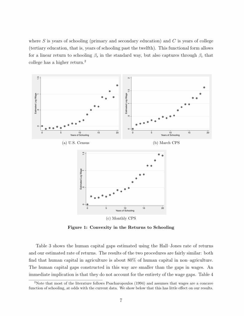
where S is years of schooling (primary and secondary education) and C is years of college
(tertiary education, that is, years of schooling past the twelfth). This functional form allows
for a linear return to schooling βs in the standard way, but also captures through βc that
college has a higher return.2
0.5
11.
5Es
timat
ed L
og-W
age
0 5 10 15 20Years of Schooling
(a) U.S. Census
0.5
11.
52
Estim
ated
Log
-Wag
e
0 5 10 15 20Years of Schooling
(b) March CPS
0.5
11.
5Es
timat
ed L
og-W
age
0 5 10 15 20Years of Schooling
(c) Monthly CPS
Figure 1: Convexity in the Returns to Schooling
Table 3 shows the human capital gaps estimated using the Hall–Jones rate of returns
and our estimated rate of returns. The results of the two procedures are fairly similar: both
find that human capital in agriculture is about 80% of human capital in non–agriculture.
The human capital gaps constructed in this way are smaller than the gaps in wages. An
immediate implication is that they do not account for the entirety of the wage gaps. Table 4
2Note that most of the literature follows Psacharopoulos (1994) and assumes that wages are a concavefunction of schooling, at odds with the current data. We show below that this has little effect on our results.
7

Table 3: Standard Estimates of Human Capital Gaps (U.S. 1980–2011)
U.S. Census March CPS Monthly CPS
Hall–Jones Rate of Return 0.80 0.81 0.80
Estimated Rate of Return 0.80 0.79 0.80
Table 4: Wage Gaps Adjusted for Standard Human Capital Gaps(U.S. 1980–2011)
U.S. Census March CPS Monthly CPS
Hall–Jones Rates of Return 0.72 0.70 0.69
Estimated Rates of Return 0.72 0.67 0.69
makes this point precise. The line entitled “estimated rate of return” shows the unaccounted
for wage gaps, that is, the remaining gaps in the level of wages between agriculture and
non–agriculture after netting out the effects of schooling. Agriculture is still estimated to
offer roughly 30% lower wages than non–agriculture. To understand why, we now develop
a simple model of sectoral wages and human capital which is going to guide the next steps
of our empirical analysis.
3 Model
3.1 Environment
Consider a static environment with L > 0 individuals. Each individual is endowed with
one unit of time, an innate ability x and non–negative numbers of years of schooling s ≥ 0.
Denote by Ω the two–dimensional set of individual characteristics.
There is an agricultural and non–agricultural consumption good. Individual preference
over the consumption of the two goods are represented by the following utility function:
u(ca, cn) = α log(ca) + (1− α) log(cn) (1)
where the superscripts indicate the sector and α ∈ (0, 1) is a relative weight. For simplicity,
we will assume that individuals do not value leisure, implying that in equilibrium they will
allocate their full time endowment to work.
The two goods are produced according to linear production functions that use labor as
8

the only input factor:
Y i = AiH i (2)
Ai denotes TFP, which here is the same as labor productivity, and H i denotes human
capital in sector i:3
H i =
∫Ω
νi(x, s)hi(x, s)dµ(x, s) (3)
where νi(x, s) is an indicator function that equals one if individual (x, s) works in sector
i. hi(x, s) is the human capital of individual (x, s) in sector i. For future reference, we
denote the number of individuals in sector i by Li. Note that when we estimated H i above,
we imposed that the returns to schooling are the same in both sectors. This is the case
if ha(x, s) = hn(x, s). In general, however, there is no reason to restrict hi(x, s) to be the
same in both sectors, so we don’t impose this on the model from the start.
The development literature considers barriers/wedges that prevent the free movement
of labor from agriculture to non–agriculture and distort the efficient allocation of labor
between the two sectors. A simple way of capturing the effects of such barriers on the
allocation of labor is to assume that there is a government that imposes a tax τ on wages
in non–agriculture and redistributes the proceeds through a lump–sum transfer T to all
individuals. This is similar to the way in Restuccia et al. (2008) modeled barriers.
3.2 Equilibrium definition
A competitive equilibrium in this model world is goods prices (P a, P n) (one of which is set
to one reflecting the choice of numeraire), rental rates (W a,W n), a tax rate τ , choices of
consumption and sector (ca, cn, νa, νn)(x, s)(x,s)∈Ω, output and labor in each sector Y i, H i
such that:
• ∀(x, s) ∈ Ω, (ca, cn, νa, νn)(x, s) solve the individual problem:
maxca,cn,νa,νn
α log(ca) + (1− α) log(cn) (4)
s.t. P aca + P ncn = W aha(x, s)νa + (1− τ)W nhn(x, s)νn + T
3Note that Hi is sometimes referred to as efficiency units in sector i.
9

• (Y i, H i) solve the firm problem in sector i:
maxY,H
P iY −W iH s.t. Y = AiH (5)
• Markets clear:
Y i =
∫Ω
ci(x, s)dµ(x, s) (6)
H i =
∫Ω
νi(x, s)hi(x, s)dµ(x, s) (7)
One might be tempted to start solving this model by requiring that the rental rates
of human capital are equalized across sectors, W a = W n. For two reasons this is not
necessarily an equilibrium property of our simple model. The first one is that the W i’s
have to adjust in such a way that the labor market clears and the “right” number of
individuals chooses each sector. The second reason is that we have assumed that only W n
is taxed, implying that W n > W a even if the net wages were equalized across sectors,
(1− τ)W n = W a.
3.3 Equilibrium sorting
Since in the data individuals in non–agriculture have more years of schooling, we are in-
terested in equilibria in which individuals sort according to their characteristics. To ensure
that such an equilibrium exists and is unique in our model, we need to impose more struc-
ture on the environment. Suppose, first, that schooling is a continuous and increasing
function of the innate ability, s(x), s′(x) ≥ 0. This would result endogenously in a dynamic
version of this model where individuals optimally choose schooling.
If positive measures of individuals work in each sector, then there must at least be
one individual xl who weakly prefers agriculture and one individual xh who prefers non–
agriculture:
W aha(xl, s(xl)) ≥ (1− τ)W nhn(xl, s(xl)) (8)
W aha(xh, s(xh)) ≤ (1− τ)W nhn(xh, s(xh)) (9)
Continuity then implies that there must be an indifferent individual (x∗, s(x∗)) with:
W aha(x∗, s(x∗)) = (1− τ)W nhn(x∗, s(x∗))
10

Note that if
ha(x∗, s(x∗)) 6= hn(x∗, s(x∗))
then
W a 6= (1− τ)W n
that is, the rental rates of efficiency units may differ in our model even if there is no tax
distortion. The reason for this, of course, is that if the technologies that translate individual
characteristics into human capital differ across sectors, then the net wage per efficiency unit
needs to be higher in the sector in which individual (x∗, s(x∗))’s human capital is lower.
This is important to keep in mind, particularly since some contributors to the literature act
as if efficiency (here τ = 0) was the same as the equalization of the rental rates of efficiency
units across sectors.
Given the evidence collected in the previous section, it is natural to focus on a sorting
equilibrium in which all individuals with x < x∗ choose agriculture and all individuals with
x > x∗ choose non–agriculture. Sufficient conditions for the existence of such a sorting
equilibrium are that:4
dhi(x, s(x))
dx≥ 0 (10)
and that for each indifferent individual
dha(x∗, s(x∗))
dx≤ dhn(x∗, s(x∗))
dx(11)
where dhi/dx is the total derivative of hi with respect to x. Condition (10) will typically be
satisfied in dynamic models in which individuals choose their years of schooling optimally,
trading off the return to an additional year of schooling against the foregone return of
an additional year of experience. (11) is more restrictive, as it depends on the specific
properties of the hi functions.
Without going into further detail in this regard, we are now in a position to state several
properties of sorting equilibria in our model that will help us interpret what we find in the
data and guide our further analysis. Suppose that positive numbers of individuals choose
each sector and that
ha(x, s(x)) ≤ hn(x, s(x)) (12)
4Uniqueness follows if all inequalities are strict.
11

i.e., for each ability x human capital is at least as high in non–agriculture than in agriculture.
Then it must be that
W a = W n ⇐⇒ ha(x, s(x)) = hn(x, s(x)) and τ = 0 (13)
that is, the rental rates of human capital are the same in both sectors if and only if the
technologies that translate characteristics into human capital are the same in both sectors
and the allocation of labor is efficient. In this case, all individuals are indifferent in our
model. We can still sort them such that individuals with x < x∗ work in agriculture and
individuals with x > x∗ work in non–agriculture. In such a sorting equilibrium, the average
wage is larger in non–agriculture than in agriculture:
W aHa
La<W nHn
Ln(14)
As we will see in the next section, this case accounts for the wage gap between non–
agriculture and agriculture in the U.S. In order to establish this, we will estimate W i and
show that W a = W n. The next proposition summarizes the results derived thus far:
Proposition 1. Suppose that (8)–(12) hold and that τ ≥ 0. If W a = W n, then:
(i) ha(x, s(x)) = hn(x, s(x))
(ii) Ha < Hn
(iii) W aHa/La < W nHn/Ln
(iv) τ = 0
In the other case, i.e. W a 6= W n and ha(x, s(x)) ≤ hn(x, s(x)), it is impossible in general
to make statements about hi(x, s(x)) and τ . However, if the technologies are the same, then
we have the following useful result:
Proposition 2. Suppose that (8)–(11) hold and ha(x, s(x)) = hn(x, s(x)). Then:
(i) (1− τ) = W a/W n
(ii) If W a < W n, then τ = (W n −W a)/W n ∈ (0, 1).
This Proposition will have important implications for interpreting the international findings
below.
12
4 Further Facts about Sectoral Wages and Human
Capital in the U.S.
4.1 Mincer returns by sectors (U.S. 1980–2011)
The standard way of constructing human capital, which we followed when we estimated
adjusted wage gaps in section 2, assumes that the value of a year of schooling is the same
in agriculture and non–agriculture. The model section above suggests that this may be
overly restrictive. We therefore assess now whether the Mincer returns to education differ
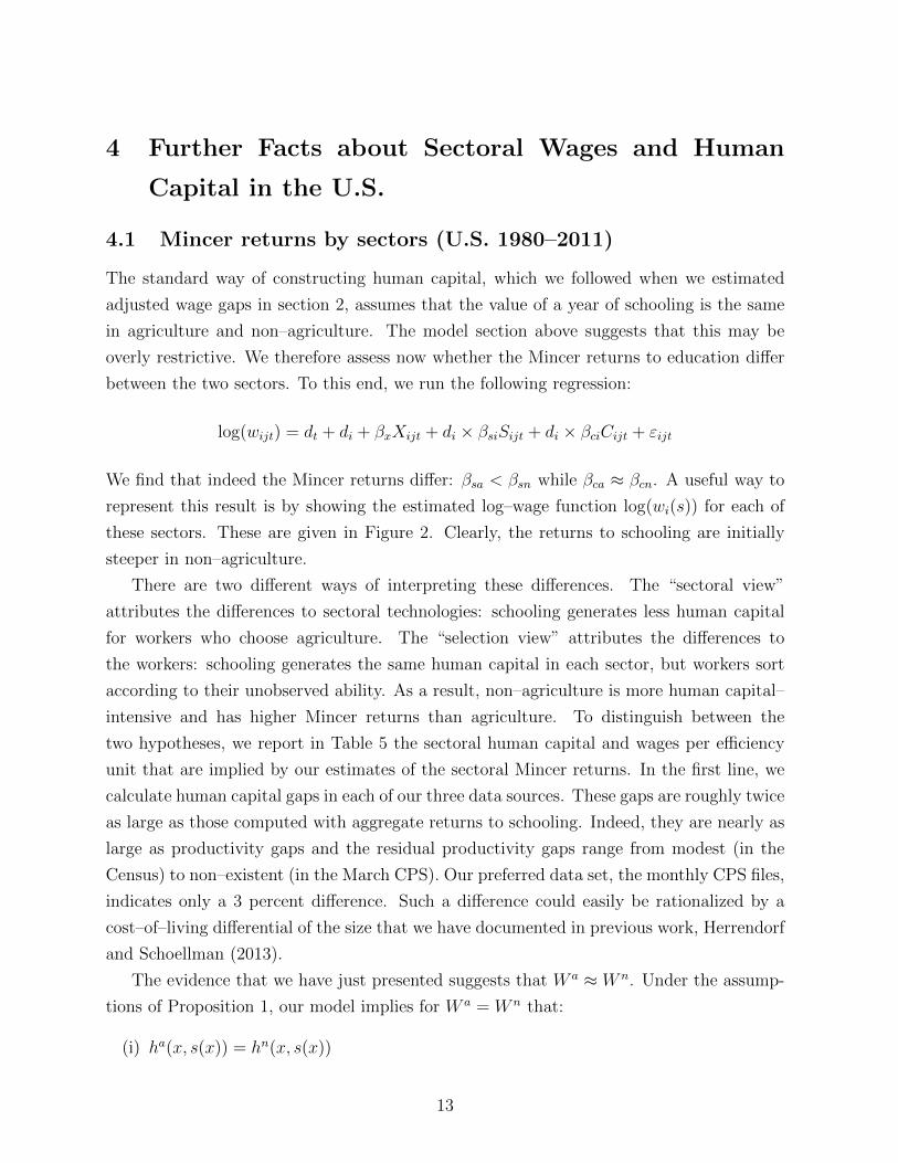
between the two sectors. To this end, we run the following regression:
log(wijt) = dt + di + βxXijt + di × βsiSijt + di × βciCijt + εijt
We find that indeed the Mincer returns differ: βsa < βsn while βca ≈ βcn. A useful way to
represent this result is by showing the estimated log–wage function log(wi(s)) for each of
these sectors. These are given in Figure 2. Clearly, the returns to schooling are initially
steeper in non–agriculture.
There are two different ways of interpreting these differences. The “sectoral view”
attributes the differences to sectoral technologies: schooling generates less human capital
for workers who choose agriculture. The “selection view” attributes the differences to
the workers: schooling generates the same human capital in each sector, but workers sort
according to their unobserved ability. As a result, non–agriculture is more human capital–
intensive and has higher Mincer returns than agriculture. To distinguish between the
two hypotheses, we report in Table 5 the sectoral human capital and wages per efficiency
unit that are implied by our estimates of the sectoral Mincer returns. In the first line, we
calculate human capital gaps in each of our three data sources. These gaps are roughly twice
as large as those computed with aggregate returns to schooling. Indeed, they are nearly as
large as productivity gaps and the residual productivity gaps range from modest (in the
Census) to non–existent (in the March CPS). Our preferred data set, the monthly CPS files,
indicates only a 3 percent difference. Such a difference could easily be rationalized by a
cost–of–living differential of the size that we have documented in previous work, Herrendorf
and Schoellman (2013).
The evidence that we have just presented suggests that W a ≈ W n. Under the assump-
tions of Proposition 1, our model implies for W a = W n that:
(i) ha(x, s(x)) = hn(x, s(x))
13

0.5
11.
52
Estim
ated
Log
-Wag
e
0 5 10 15 20Years of Schooling
Non-Agriculture Agriculture
(a) U.S. Census
0.5
11.
52
Estim
ated
Log
-Wag
e
0 5 10 15 20Years of Schooling
Non-Agriculture Agriculture
(b) March CPS
0.5
11.
52
Estim
ated
Log
-Wag
e
0 5 10 15 20Years of Schooling
Non-Agriculture Agriculture
(c) Monthly CPS
Figure 2: Returns to Schooling Vary by Sector
(ii) Ha < Hn
(iii) W aHa/La < W nHn/Ln
(iv) τ = 0
That is, in this case our model accounts for the key features in the U.S. data. Interestingly,
(iv) implies in the context of our model that the allocation of labor between non–agriculture
and agriculture is efficient, which is what the literature on structural transformation as-
sumes, at least for the U.S. Implication (i) that ha(x, s(x)) = hn(x, s(x)) is rather restrictive.
In the next subsection, we provide evidence from individuals who switch sector (“switch-
ers”) that is broadly consistent with (i).
14

Table 5: Gaps Measured with Sector–specific Returns to School-ing (U.S. 1980–2011)
U.S. Census March CPS Monthly CPS
Human Capital Gaps 0.65 0.52 0.57
Residual Wage Gaps 0.88 1.00 0.97
4.2 Mincer returns for switchers (U.S. 1980–2011)
We now study the wage patterns of workers who switch sectors (“switchers”). If workers
who switch sectors experience large changes in the return on their education, this indicates
that the differences are intrinsic to the sectoral technology. This would contradict the
conclusions derived so far. If workers who switch sectors do not experience large changes
in the return on their education, this indicates that they are intrinsic to the workers. This
would support the conclusions derived so far.
Our ideal data set has a panel dimension so that we can compare the wages and wage
structure before and after switching industries for the same worker. Our ideal data set
also has a large sample so that we can observe a sufficient number of switchers, given the
relatively small size of the agricultural labor force in the U.S. today. The only dataset
that we are aware of that satisfies these requirements is the CPS. The CPS provides the
sample size that we need and includes a short panel structure: households are in the CPS
for four months, then out for eight months, before returning for four more months. We
focus on matching the fourth month of each spell, when extra data are collected (the so–
called “outgoing rotation groups”). These two observations are separated by one year. We
can study the changes in wages and wage structure for workers who switch sectors in the
intervening year.
Matching workers over time in the CPS is well known to be challenging. The basic
problem stems from two points. First, the CPS is really a survey of addresses, not persons
or households. That is, the CPS samples dwellings based on address and surveys whoever
lives in that dwelling. In some cases, the family in that dwelling will differ over time. In
principle the CPS carefully denotes when such of household change within a dwelling occurs.
However, the second point is that the within–dwelling household and person identifiers are
known to have coding errors. Fortunately, there is a well-established procedure for dealing
with these issues and matching the CPS that we follow here (Madrian and Lefgren 1999,
Madrian and Lefgren 2000). The basic idea is to start by matching all persons who share
the same dwelling, household, and person identifiers. We then check whether the match
15

Table 6: Wage Gaps for Matched and Unmatched Sam-ples (U.S. 1980–2011)
Monthly CPS Matched CPS
Raw Wage Gap 0.58 0.53
Adjusted Wage Gap 0.55 0.49
Standard Human Capital 0.69 0.63
Sector-Specific Returns 0.97 0.96
is valid by checking whether variable responses are logically consistent across time within
a match. Here, there is a tradeoff. If one checks more variables and/or requires stricter
agreement over time, then one excludes more false matches, but also excludes some valid
matches where a code is misreported. We adopt a fairly strict check by requiring that age,
sex, and race all agree.5
The matching process excludes a number of observations. Before analyzing the data,
we want to make certain that the same basic facts apply also in the sample of matched
workers. If so, then we can be reassured at least that workers we can match do not differ
in obvious ways from the workers we exclude. We focus on two moments that are of the
most interest to our analysis. First is the wage gap. Table 6 shows the raw wage gap that
prevails in the monthly CPS and the matched CPS. The two should agree closely because
they start with the same observations; the only difference is that the matched file contains
only households that can be matched across years. Indeed the gap is close in size. The Table
also shows the gap after making a series of adjustments for state and gender; for schooling,
using the observed aggregate return; and for schooling, using the observed sectoral return.
Throughout the estimates are close. This is reassuring because it says that the matching
process yields a dataset with wage gaps similar to the baseline data.
Given our interest in the sectoral return to schooling we also check whether the basic
patterns are the same for matched and unmatched data sets. We estimate the same equation
allowing for sectoral returns to schooling in each dataset and plot the resulting wage as a
function of schooling profiles in Figure 3. The two profiles are indeed quite similar, again
reassuring us that the results we find for the matched CPS will apply to the other U.S.
data sets discussed in the previous section.
Having established that the matched CPS appears to be a useful dataset to study, we
5Agreement here means that the gender is the same; that the race report of white or non–white is thesame; and that the age in the later period is between the same and two years older than the age in theearlier period. Note that since the CPS is not necessarily asked on the exact same date of the month eachtime, this is the strictest agreement on age that one can check.
16

0.5
11.
52
Estim
ated
Log
-Wag
e
0 5 10 15 20Years of Schooling
Non-Agriculture Agriculture
(a) Monthly CPS
0.5
11.
52
Estim
ated
Log
-Wag
e
0 5 10 15 20Years of Schooling
Non-Agriculture Agriculture
(b) Matched CPS
Figure 3: Sectoral Return to Schooling in Matched and Unmatched CPS Data
Table 7: Wage Changes for Stayers and Switchers(U.S. 1980–2011)
a→a a→n n→a n→n
0.05 0.22 -0.08 0.07
now turn to analyzing the experiences of switchers and non–switchers. We define four
groups: those who work in agriculture both years; those who work in non–agriculture both
years; those who switch from agriculture to non–agriculture; and those who switch from
non–agriculture to agriculture. We focus on the determinants of the annual changes in
wages. That is, we want to understand for worker i who works in sectors j and j′ in periods
t and t − 1 the determinants of ∆ log(wijj′t) ≡ log(wijj′t) − log(wijj′t−1). As a simple
exploratory regression we try:
∆ log(wijj′t) = βdjj′djj′ + βddt + εijj′t.
where jj′ denotes a sector pair; for example, jj′ = a, a denotes workers who stay in agricul-
ture, and jj′ = n, a denotes workers who switch from non–agriculture to agriculture. The
idea of this regression is simply to capture the mean effect of staying in the same sector
versus switching, controlling for trend wage growth with dt.
Table 7 shows the resulting estimates. Workers who remain in agriculture and non–
agriculture gain roughly 5 and 7 percent higher wages. The more interesting figure is for
switchers: workers who switch from agriculture to non–agriculture gain roughly 22 percent
17

higher wages, while workers who switch in the opposite direction lose roughly 8 percent
of their wages. These figures are quite small relative to the total agricultural wage gap of
roughly 40 percent. We view these results as providing evidence that most of wage gaps
represent selection of workers of different types. When an identical worker is moved, the
wage gap moves by (on average) just 15 percent.
A common concern is selection. One can imagine that all workers have the chance to
switch sectors and that there is some heterogeneity in the wage gain or loss to switching
sectors. In most models, workers with larger gains (or smaller losses) will be more likely
to switch. This logic suggests (for example) that the 8 percent wage loss from moving to
agriculture from non–agriculture may understate the wage loss that would occur if a random
sample of workers were moved. Note, however, that the same logic works in reverse: the
22 percent wage gain from moving from agriculture to non-agriculture is probably higher
than the wage gain that would occur if a random sample of workers were moved. A simple
bounding argument suggests that the underlying wage difference between agriculture and
non–agriculture is between 8 and 22 percent.
We now ask how switching affects the market value of education. Recall that the
cross–sectional estimates indicate higher returns to education than in non–agriculture in
agriculture. The estimated wage–schooling relationship for the two sectors is given in Figure
4a. The relationships in the matched CPS data suggest large differences in the return to
education. In Figure 4b we add the returns to education for those who switch, as observed
before the switch. We can see already that switchers are different even before they switch:
their wage–return on their education is between that of workers who stay in agriculture
and workers who stay in non-agriculture. This evidence suggests that selection may play a
role. In Figure 4c, we confirm this suspicion: the value of education after switching is still
between the two sectors, and not too different from the value of education before switching.
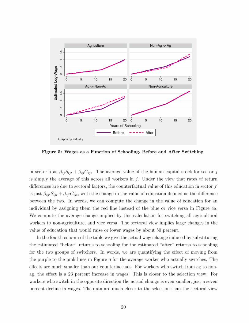
This last fact may be better represented by Figure 5, which shows, group by group,
the value of education before and after. For workers who remain in agriculture or non–
agriculture throughout the value is essentially unchanged. For workers who switch sectors,
the changes are modest: workers who exit agriculture earn somewhat higher returns on
their schooling, while workers who switch to agriculture experience almost no change in the
relevant region. These two figures indicate that much of the gap in the return to schooling
is attributable to selection: workers who are going to switch are already different from
non–switchers in the same sector. Further, when switchers switch, their returns change
little.
It may be useful to provide a quantitative sense of how much the data support the
18

0.5
11.
52
Estim
ated
Log
-Wag
e
0 5 10 15 20Years of Schooling
Non-Agriculture Agriculture
(a) Stayers
0.5
11.
52
Estim
ated
Log
-Wag
e
0 5 10 15 20Years of Schooling
Non-Agriculture AgricultureNon-Ag -> Ag Ag -> Non-Ag
(b) Stayers and Switchers (Before)
0.5
11.
52
Estim
ated
Log
-Wag
e
0 5 10 15 20Years of Schooling
Non-Agriculture AgricultureNon-Ag -> Ag Ag -> Non-Ag
(c) Stayers and Switchers (After)
Figure 4: Sectoral Return to Schooling for Switchers and Stayers
“sectoral differences” versus “selection” views of why returns to schooling differ across
sectors. We can perform a simple calculation that gives such a sense. The idea is to
quantify the total change in the value of education that one would observe under each of
these theories; to compute the actual change observed in the data; and then to compare
the three values to assess how close the data is to each theory.
For the “selection” view, the answer is straightforward: rates of return differences reflect
differences in the workers who select into the two sectors. When workers switch they take
their returns with them. Hence, switchers would experience no change in the value of their
education. This value is reported in column 2 of Table 8.
For the “sectoral” view, the answer requires some calculation. We observe in the data
Sijt, Cijt, βsj, and βcj. We can compute the total value of the schooling for a worker i
19
0.5
11.
50
.51
1.5
0 5 10 15 20 0 5 10 15 20
0 5 10 15 20 0 5 10 15 20
Agriculture Non-Ag -> Ag
Ag -> Non-Ag Non-Agriculture
Before After
Estim
ated
Log
-Wag
e
Years of Schooling
Graphs by Industry
Figure 5: Wages as a Function of Schooling, Before and After Switching
in sector j as βsjSijt + βcjCijt. The average value of the human capital stock for sector j
is simply the average of this across all workers in j. Under the view that rates of return
differences are due to sectoral factors, the counterfactual value of this education in sector j′
is just βsj′Sijt + βcj′Cijt, with the change in the value of education defined as the difference
between the two. In words, we can compute the change in the value of education for an
individual by assigning them the red line instead of the blue or vice versa in Figure 4a.
We compute the average change implied by this calculation for switching all agricultural
workers to non-agriculture, and vice versa. The sectoral view implies large changes in the
value of education that would raise or lower wages by about 50 percent.
In the fourth column of the table we give the actual wage change induced by substituting
the estimated “before” returns to schooling for the estimated “after” returns to schooling
for the two groups of switchers. In words, we are quantifying the effect of moving from
the purple to the pink lines in Figure 6 for the average worker who actually switches. The
effects are much smaller than our counterfactuals. For workers who switch from ag to non-
ag, the effect is a 23 percent increase in wages. This is closer to the selection view. For
workers who switch in the opposite direction the actual change is even smaller, just a seven
percent decline in wages. The data are much closer to the selection than the sectoral view
20
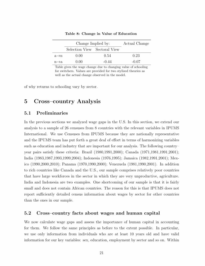
Table 8: Change in Value of Education
Change Implied by: Actual Change
Selection View Sectoral View
a→n 0.00 0.54 0.23
n→a 0.00 -0.44 -0.07
Table gives the wage change due to changing value of schoolingfor switchers. Values are provided for two stylized theories aswell as the actual change observed in the model.
of why returns to schooling vary by sector.
5 Cross–country Analysis
5.1 Preliminaries
In the previous sections we analyzed wage gaps in the U.S. In this section, we extend our
analysis to a sample of 26 censuses from 8 countries with the relevant variables in IPUMS
International. We use Censuses from IPUMS because they are nationally representative
and the IPUMS team has put forth a great deal of effort in terms of harmonizing variables
such as education and industry that are important for our analysis. The following country–
year pairs satisfy these criteria: Brazil (1980,1991,2000); Canada (1971,1981,1991,2001);
India (1983,1987,1993,1999,2004); Indonesia (1976,1995); Jamaica (1982,1991,2001); Mex-
ico (1990,2000,2010); Panama (1970,1990,2000); Venezuela (1981,1990,2001). In addition
to rich countries like Canada and the U.S., our sample comprises relatively poor countries
that have large workforces in the sector in which they are very unproductive, agriculture.
India and Indonesia are two examples. One shortcoming of our sample is that it is fairly
small and does not contain African countries. The reason for this is that IPUMS does not
report sufficiently detailed census information about wages by sector for other countries
than the ones in our sample.
5.2 Cross–country facts about wages and human capital
We now calculate wage gaps and assess the importance of human capital in accounting
for them. We follow the same principles as before to the extent possible. In particular,
we use only information from individuals who are at least 10 years old and have valid
information for our key variables: sex, education, employment by sector and so on. Within
21
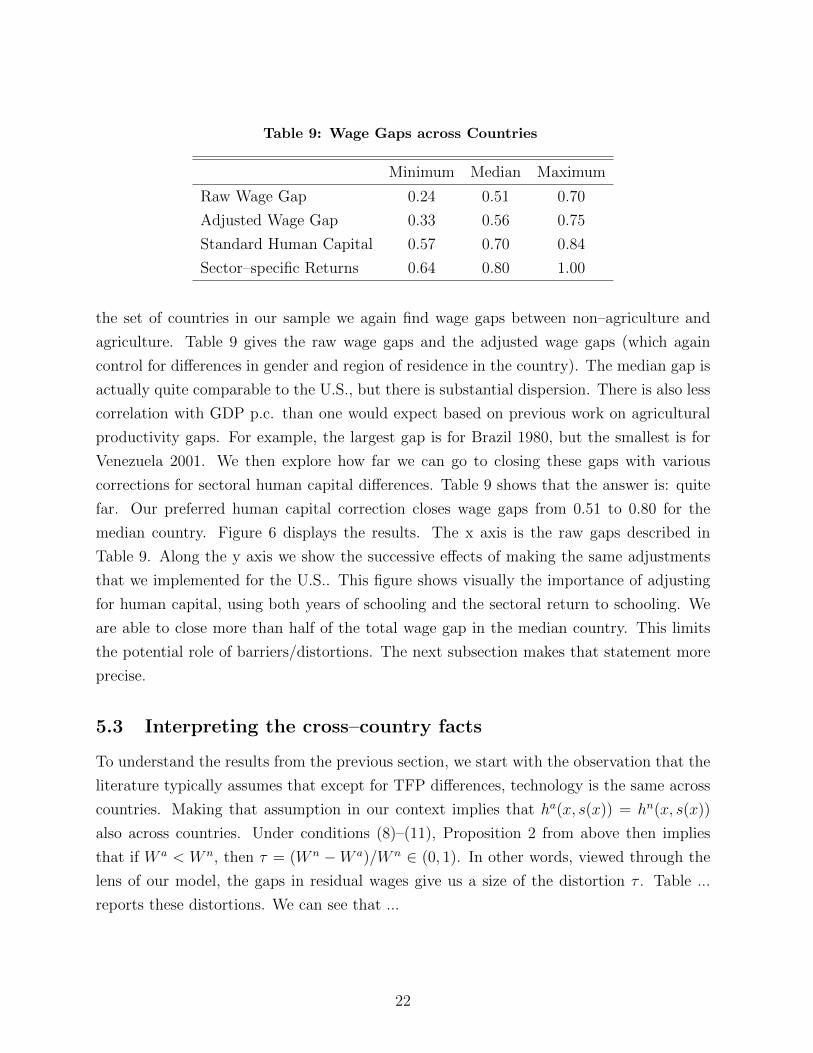
Table 9: Wage Gaps across Countries
Minimum Median Maximum
Raw Wage Gap 0.24 0.51 0.70
Adjusted Wage Gap 0.33 0.56 0.75
Standard Human Capital 0.57 0.70 0.84
Sector–specific Returns 0.64 0.80 1.00
the set of countries in our sample we again find wage gaps between non–agriculture and
agriculture. Table 9 gives the raw wage gaps and the adjusted wage gaps (which again
control for differences in gender and region of residence in the country). The median gap is
actually quite comparable to the U.S., but there is substantial dispersion. There is also less
correlation with GDP p.c. than one would expect based on previous work on agricultural
productivity gaps. For example, the largest gap is for Brazil 1980, but the smallest is for
Venezuela 2001. We then explore how far we can go to closing these gaps with various
corrections for sectoral human capital differences. Table 9 shows that the answer is: quite
far. Our preferred human capital correction closes wage gaps from 0.51 to 0.80 for the
median country. Figure 6 displays the results. The x axis is the raw gaps described in
Table 9. Along the y axis we show the successive effects of making the same adjustments
that we implemented for the U.S.. This figure shows visually the importance of adjusting
for human capital, using both years of schooling and the sectoral return to schooling. We
are able to close more than half of the total wage gap in the median country. This limits
the potential role of barriers/distortions. The next subsection makes that statement more
precise.
5.3 Interpreting the cross–country facts
To understand the results from the previous section, we start with the observation that the
literature typically assumes that except for TFP differences, technology is the same across
countries. Making that assumption in our context implies that ha(x, s(x)) = hn(x, s(x))
also across countries. Under conditions (8)–(11), Proposition 2 from above then implies
that if W a < W n, then τ = (W n −W a)/W n ∈ (0, 1). In other words, viewed through the
lens of our model, the gaps in residual wages give us a size of the distortion τ . Table ...
reports these distortions. We can see that ...
22

.2.4
.6.8
1Ad
just
ed W
age
Gap
.2 .4 .6 .8 1Raw Wage Gap
Cumulative Adjustment for: Geography and GenderSchooling Sector-Specific Return
Figure 6: Wage Gaps and Adjusted Wage Gaps
6 Discussion
6.1 Relation to the literature
Our results are related to Gollin, Lagakos and Waugh (2011), who seek to measure and
account for gaps between non–agricultural and agricultural productivity. The main differ-
ence between the two papers is that Gollin et al. focus on a much larger set of countries
including the poorest ones from Africa. While that makes their sample more representative
than ours, the wage data by sector from population censuses that we use here do not exist
for most of their countries. They therefore use Mincer returns that are common across all
countries to construct measures of human capital gaps across sectors. Since we have wage
data by country and sector, we use the estimated Mincer returns by sector instead. We find
that the human capital gaps constructed with estimated Mincer returns are considerably
larger than those constructed with the Mincer returns used by Gollin et al. (2011).
Our results are also related to Young (2013), who documented for 65 poor and middle–
income countries that migration flows go in both directions: while on average one in five
individuals born in rural areas moves to urban areas as an adult, one in four individuals born
in urban areas moves to rural areas as an adult. Young develops a location model in which
23

people sort depending on observed characteristics such as schooling and on unobserved
characteristics such as skills that are acquired after leaving school. The basic idea is that if
observed and unobserved characteristics are positively correlated and are more important
as an input in production in urban areas, then sorting implies that on average individuals
with higher observed and unobserved characteristics locate in urban areas and individuals
with lower observed and unobserved characteristics locate in rural areas. Since our concept
of human capital is broad in the sense that it includes the stocks of observed and unobserved
characteristics, this prediction of Young is consistent with our finding that most of the wage
gaps between non–agriculture and agriculture are accounted for by the fact that workers in
non–agriculture have considerably more human capital (broadly measured).
6.2 Implications for the Macro–Development Literature
Our work has several important implications for the macro–development literature. First,
it implies that to construct human capital at the sectoral level one needs to use Mincer
returns that are estimated at the sector level, instead of Mincer returns that are estimated
at the aggregate level. The reason for this is that Mincer returns that are estimated
at the sectoral level capture that unobserved characteristics differ across sectors, which
Mincer returns that are estimated at the aggregate level miss by construction. Second, our
result that in the U.S. wages per efficiency unit are equalized between non–agriculture and
agriculture is a necessary condition for the efficient allocation of labor between the two
sectors, which the literature on structural transformation assumes. Note, however, that
it is not a sufficient condition for efficiency because it does not rule out distortions that
indirectly affect the allocation of labor without affecting wages, an example being value
added taxes or subsidies that affect the two sectors different. Third, our result that even
in the poorer countries of our sample the potential role for distortions/barriers is relatively
small limits the quantitative importance of surplus labor in agriculture ...
7 Conclusion
We have documented for eight countries ranging from rich (Canada, U.S.) to poor (India,
Indonesia) that average wages are considerably higher in non–agriculture than in agricul-
ture. We have proposed a measure of human capital at the sector level that accounts for
the entire wage gap in the U.S. and most of the wage gaps elsewhere. The key feature of
this measure has been that Mincer returns to schooling were estimated at the sectoral level,
24

instead of at the aggregate level. We have developed a multi-sector model that explains
these finding if: (i) Mincer returns to schooling are equal in both sectors; (ii) more able
workers sort into non–agriculture; (iii) distortions to the allocation of labor between sectors
are zero in the U.S. and small elsewhere. We have argued that (iii) implies that the role
for misallocation of labor between non–agriculture and agriculture is rather limited.
Our work opens several interesting avenues for future research ...
References
Bils, Mark and Peter J. Klenow, “Does Schooling Cause Growth?,” American Eco-
nomic Review, December 2000, 90 (5), 1160–1183.
Binelli, Chiara, “How the Wage-Education Profile got More Convex: Evidence from
Mexico,” 2012. mimeo, University of Southampton.
Caselli, Francesco, “Accounting for Cross-Country Income Differences,” in Philippe
Aghion and Steven N. Durlauf, eds., Handbook of Economic Growth, Vol. 1A, Elsevier,
2005, chapter 9, pp. 679–741.
Gollin, Doug, David Lagakos, and Mike Waugh, “The Agricultural Productivity Gap
in Developing Countries,” 2011. mimeo, Arizona State University.
Hall, Robert E. and Charlies I. Jones, “Why Do Some Countries Produce So Much
More Output Per Worker Than Others?,” Quarterly Journal of Economics, February
1999, 114 (1), 83–116.
Herrendorf, Berthold and Todd Schoellman, “Why is Measured Productivity So Low
in Agriculture?,” 2013. mimeo, Arizona State University.
, Richard Rogerson, and Akos Valentinyi, “Growth and Structural Transforma-
tion,” in Philippe Aghion and Steven N. Durlauf, eds., Handbook of Economic Growth,
Vol. 2, Elsevier, 2013, pp. 855–941.
Kuznets, Simon, “Modern Economic Growth: Findings and Reflections,” Amercian Eco-
nomic Review, 1973, 63, 247–258.
Lemieux, Thomas, “The Mincer Equation Thirty Years After Schooling, Experience, and
Earnings,” in S. Grossbard, ed., Jacob Mincer, A Pioneer of Modern Labor Economics,
Springer Verlag, 2006, pp. 127–145.
25

Madrian, Brigitte C and Lars John Lefgren, “An approach to longitudinally match-
ing Current Population Survey (CPS) respondents,” Journal of Economic and Social
Measurement, 2000, 26 (1), 31–62.
and Lars Lefgren, “A note on longitudinally matching Current Population Survey
(CPS) respondents,” 1999. NBER Working Paper t0247.
Psacharopoulos, George, “Returns to Investment in Education: A Global Update,”
World Development, 1994, 22, 1325–1343.
Restuccia, Diego, Dennis T Yang, and Xiaodong Zhu, “Agriculture and Aggregate
Productivity: A Quantitative Cross-Country Analysis,” Journal of Monetary Eco-
nomics, March 2008, 55 (2), 234–250.
Young, Alwyn, “Inequality, the Urban-Rural Gap, and Migration,” The Quarterly Jour-
nal of Economics, 2013, 128 (4), 1727–1785.
Data Appendix
26