Vulnerability of wetlands to climate change in the Southern Interior Ecoprovince: a preliminary assessment1

Final Report

Fred L. Bunnell Ralph Wells Arnold Moy

Centre for Applied Conservation Research, University of British Columbia, Vancouver, B.C.

March 2010

1 This project was funded by BC Forest Sciences Program Y102120, Ducks Unlimited Canada and Environment Canada.

i

EXECUTIVE SUMMARY

As well as providing significant ecosystem services, small lakes and wetlands provide important habitat for many species, including some that are considered at risk. Wetlands also are vulnerable to the continuing effects of climate change, particularly drying trends. Relative vulnerability to climate change was assessed for 31,877 wetlands covering about 35,000 ha in the Southern Interior Ecoprovince. The drying index used to estimate vulnerability incorporated snowpack (and index of water input) and the summer heat moisture index (an approximate surrogate for evapotranspiration and water output). Using ECHAM-5 to project climate under two plausible scenarios produced strong effects on the relative vulnerability of wetlands to climate change. Likely outcomes are illustrated by shifts in deciles of the drying index values. Deciles are calculated over the entire range of projected values for a given IPCC scenario. IPCC scenario A2 is “status quo”; the B1 scenario includes efforts at mitigating greenhouse gas emissions. For both area and number of wetlands, values of the drying index shift from lower to higher deciles in future time periods. More extreme (and non-linear) shifts occur under the A2 scenario than under the B1 scenario. During ‘climate normal’ (1960s through 1990s), about 98% of the area for the smallest wetlands (<1 ha) is in deciles 1 through 4. Under the A2 projection, that proportion has declined to <40% by 2080. Over the same period, the number of small wetlands in deciles 1 through 4 declines from about 91% to 39%. Future conditions are less severe under the B1 scenario, illustrating the projected importance of mitigation efforts. By 2080, under the A2 scenario, the majority of both number and area of small wetlands are projected to experience drying indices in the 5th decile or higher; there is no longer any representation in decile 1. We expect that wetlands in deciles 8 through 9 will vanish and those in decile 7 are extremely threatened. The projected outcomes are troubling because the smallest wetlands are the most vulnerable and these comprise 67.7% of current wetlands. At least two species at risk, Great Basin Spadefoot and Tiger Salamander, exploit small, shallow wetlands. More broadly, about 80 bird species rely on wetlands as their primary breeding habitat.

The simple projection employed permits refinements that would be useful in guiding conservation efforts. Chief among these are incorporating local data, teasing apart the relative impacts on snowpack and drying by geographical strata and incorporating a vegetative layer to clarify potential management options. That is, to focus more closely on particular wetland areas and the associated feasibility and opportunity for conservation action.

ii

TABLE OF CONTENTS Abstract............................................................................................................................ 1 Introduction ..................................................................................................................... 2 Study Area ....................................................................................................................... 2 Methods ........................................................................................................................... 4 Results and Discussion.................................................................................................. 6 Conclusions................................................................................................................... 12 Acknowledgements ...................................................................................................... 13 Literature Cited…..…. ................................................................................................... 13 TABLES Table 1. Area and number of wetlands and lakes found in the SIE study area by size class. .................................................................................................................................6 FIGURES Figure 1. Southern Interior Ecoprovince study area (protected areas in green). ............3 Figure 2. Lakes and wetlands in the Southern Interior Ecoprovince. ..............................4 Figure 3. Relative contribution (%) of different size classes of wetlands to total number and total area (ha) of wetlands within the Southern Interior Ecoprovince. Adjacency not invoked………………………………..……………………………………………………….….7 Figure 4. Relative distribution of Southern Interior wetlands by elevation class in terms of: a) total area and b) total number. Wetlands discrete; adjacency not invoked…………………………………………………………………………………………....8 Figure 5. Maps of the projected climate drying index for wetlands of 10 ha and less in the Southern Interior Ecoprovince for climate normal, 2020, 2050 and 2080. Projections employ ECHAM5 under the A2 scenario……………………………………………………..9 Figure 6. Maps of the projected climate drying index for wetlands of 10 ha and less in the Southern Interior Ecoprovince for climate normal, 2020, 2050 and 2080. Projections employ ECHAM5 under the B1 scenario……………………………………………….…...10 Figure 7. Area of small Southern Interior wetlands (0 – 1 ha) by drying index decile (1 = lowest risk; 10 = highest). Deciles calculated over all years of a scenario. 10th decile not shown…………………………………………………………………………………….…….11 Figure 8. Number of small Southern Interior wetlands (0 – 1 ha) by drying index decile (1 = lowest risk; 10 = highest). Deciles calculated over all years of a scenario. 10th decile not shown.…..………………………………………………………………….…….………..11

1

ABSTRACT As well as providing significant ecosystem services, small lakes and wetlands provide important habitat for many species, including some that are considered at risk. Wetlands also are vulnerable to the continuing effects of climate change, particularly drying trends. We evaluated potential future consequences for wetlands in the Southern Interior Ecoprovince (SIE) by projecting climate variables (precipitation as snow and summer heat-moisture index) that are expected to influence small lake and wetland persistence. Climate variables were projected for the study area using ClimateBC software for two scenarios developed by the IPCC (Intergovernmental Panel on Climate Change). Results indicate that small lakes and wetlands in the Southern Interior Ecoprovince will experience drying trends due to declining snow levels and increased summer drying. Drying trends were greater under the ‘status quo’ CO2 intensive scenario (A2 of IPCC), than those projected under the CO2 mitigation scenario (B1 of IPCC). The fate of wetlands in the study area depends greatly on the success of international policies to mitigate CO2 emissions. The methodology applied here extends that developed by Wells et al. (2009) for the Central Interior Ecoprovince to better expose the components of climate having the greatest effect. The approach does not address how potential effects of local topography, forest cover and other geographic variables might modify climate variables that affect the water balance of wetlands in the study area. Some suggestions for further evaluation are offered.

2

INTRODUCTION British Columbia is experiencing similar climate trends to those documented elsewhere in western North America (Mote 2003; Taylor 2005) and more globally (IPCC 2007). There are, however, significant differences in the relative rates of change among provincial Ecoprovinces; for example, northern Ecoprovinces have shown more dramatic changes in winter minimum temperatures than have southern Ecoprovinces. Some bird species already have responded to changing climate by altering their arrival and departure times, their duration in the province, the northward extension of their range and shifting their relative abundance northward (Bunnell and Squires 2005; Bunnell et al. 2005; Bunnell et al. 2010). Current warming trends are expected to continue into the future (BCWLAP 2002; Taylor 2005; IPCC 2007). As climate has changed differently within Ecoprovinces, so have the organisms’ responses to climate (Bunnell et al. 2010). Of the 9 terrestrial Ecoprovinces in British Columbia, the Southern Interior Ecoprovince has the largest number of species ranking highly within the provincial Conservation Framework (see Bunnell et al. 2009) or formally designated ‘at risk’ by CoSEWIC. Several of these (e.g., Great Basin spadefoot toad, tiger salamander, western painted turtle) are dependent on wetlands, as are many species less threatened, including numerous waterbirds. Analyses underway for waterfowl in the well-documented Central Interior wetlands suggest that the smallest wetlands and lakes in that Ecoprovince also are the most productive for waterfowl. Small, shallow wetlands and lakes are expected to be highly vulnerable to drying trends simply because they contain the least water. Actual losses will be subject to water inputs through precipitation, rivers and ground water, much of it resulting from snowpack. The Southern Interior Ecoprovince currently contains some of the warmest and driest areas of the province. Both warming and drying are likely to increase with climate change. That is cause for concern for the species populations that depend on wetlands. This study has three objectives: 1) Develop a framework that credibly links geo-referenced wetlands of the Southern Interior Ecoprovince (as described in the B.C. Watershed Atlas or the B.C. Corporate Watershed data sources) to historical and projected climate. 2) Apply climate risk factors developed in 2008-2009 to wetlands of the Southern Interior Ecoprovince, refining where possible. 3) Provide maps illustrating relative degrees of risk across wetlands of the Southern Interior Ecoprovince.

STUDY AREA The study area for evaluating the drying index is the Southern Interior Ecoprovince (SIE), a 5.8 million hectare region found in southcentral British Columbia (Figure 1). Because the Ecoprovince lies in the rain shadow of the Coast and Cascade Mountains it contains some of the warmest and driest areas of the province in summer. Air moving into the area has already lost most of its moisture on the west-facing slopes of the coastal mountains. Vegetation is dominated by three drier Biogeoclimatic zones – the Bunchgrass Zone in the lower slopes of the large basins, the Interior Douglas-fir Zone on the lower elevations of the plateau surface, and the Montane Spruce Zone on the higher elevations of the plateaus. The topography creates conditions for smaller areas of other zones: the Engelmann Spruce-Subalpine Fir Zone occurs on the higher elevation of the plateaus and highlands, the Alpine Tundra Zone occurs on the highest slopes of the Okanagan and Clear ranges, the Ponderosa Pine Zone occurs sporadically on middle slopes of

3

the large, dry basins, and the Interior Cedar - Hemlock zone occurs on the upper slopes in the northeastern area of the Ecoprovince. See Meidinger and Pojar (1991) for a description of BEC zones. Figure 1. Southern Interior Ecoprovince study area (protected areas in green). The region is rich in small lakes and wetlands (Figure 2), which provide habitat for many species, including some designated ‘at risk’. For waterfowl, Breault et al. (2007) concluded that the smaller wetlands were the most productive. We currently are re-analyzing those data to separate other potential factors, including elevation. The relationship of greater productivity in smaller wetlands (up to about 2 ha) holds across regions within the Central Interior Ecosystem – Cariboo Basin, Chicotin Plateau and Nazko Uplands. In the Southern Interior Ecosystem, small shallow ponds appear critical to species at risk. For example, the tiger salamander, breeds, and juveniles metamorphose, in water bodies sufficiently shallow that they often are semi-permanent. This may not always have been true. Fish introductions into deeper water bodies formerly used by the salamander have made those areas ineffective as rearing spots. There are clear limitations on how long the water must be available. It takes 3 to 4 months for tiger salamanders to acquire lungs and become terrestrial. Under changing climate, existing vernal water bodies could become too short-lived to contribute effectively.

4

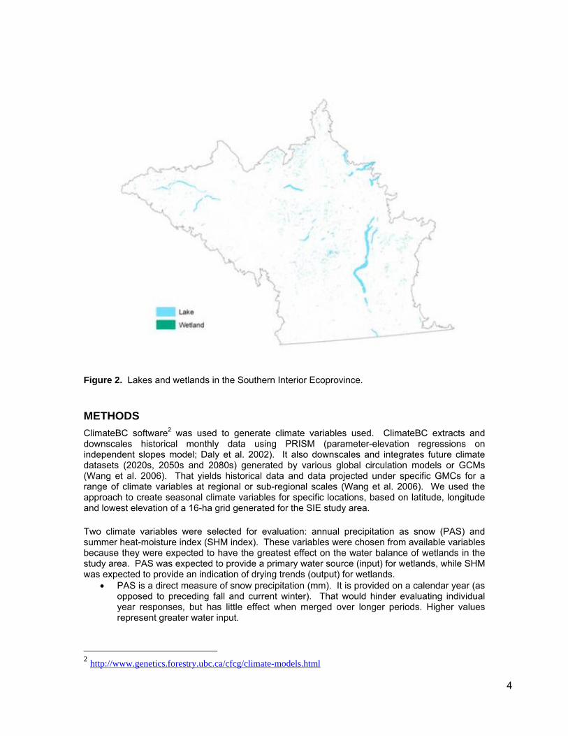
Figure 2. Lakes and wetlands in the Southern Interior Ecoprovince.

METHODS ClimateBC software2 was used to generate climate variables used. ClimateBC extracts and downscales historical monthly data using PRISM (parameter-elevation regressions on independent slopes model; Daly et al. 2002). It also downscales and integrates future climate datasets (2020s, 2050s and 2080s) generated by various global circulation models or GCMs (Wang et al. 2006). That yields historical data and data projected under specific GMCs for a range of climate variables at regional or sub-regional scales (Wang et al. 2006). We used the approach to create seasonal climate variables for specific locations, based on latitude, longitude and lowest elevation of a 16-ha grid generated for the SIE study area. Two climate variables were selected for evaluation: annual precipitation as snow (PAS) and summer heat-moisture index (SHM index). These variables were chosen from available variables because they were expected to have the greatest effect on the water balance of wetlands in the study area. PAS was expected to provide a primary water source (input) for wetlands, while SHM was expected to provide an indication of drying trends (output) for wetlands.

• PAS is a direct measure of snow precipitation (mm). It is provided on a calendar year (as opposed to preceding fall and current winter). That would hinder evaluating individual year responses, but has little effect when merged over longer periods. Higher values represent greater water input.

2 http://www.genetics.forestry.ubc.ca/cfcg/climate-models.html

5

• SHM is generated by ClimateBC using the equation: (MWMT * 1000)/MSP, where MWMT is the Mean Warmest Month Temperature (°C) and MSP is Mean Summer (May – Sept) Precipitation (mm). SHM index is a derived variable, used as a limited proxy for direct measures of humidity or evaporation and transpiration, which are often unavailable (Tuhkanen 1980). Higher values of the SHM index represent a stronger drying tendency relative to lower values (due to less precipitation and/or higher temperature).

For use as a qualitative drying index, PAS and SHM data were normalized on a 0 – 1 scale, with higher values representing a higher risk of drying (PAS was normalized on an inverse scale, as high PAS confers low risk). Before normalizing, PAS data were log-transformed because limited amounts of very high snow levels (e.g., upper elevation areas) resulted in a highly skewed distribution of PAS data. These 2 normalized values were then combined multiplicatively √(PAS x SHM) to yield a single normalized value representing a measure of the risk of drying, ranging from 0 to 1. Multiplicative combination permits either drying or lack of snowpack to have a dominating effect. For example, an area with almost no snowpack or very high heat moisture index may be under much greater drying stress than an area with average levels of both variables. An additive index would not distinguish between these two conditions. When deciles are presented they are calculated for all time periods within a particular scenario. To assess vulnerability PAS and SHM variables were projected for a baseline ‘climate normal’ period (1960-1990) using downscaled PRISM data, and for two future scenario’s representing differing levels of future global CO2 production. Future scenarios selected for projection were the Intergovernmental Panel on Climate Change (IPCC) A2 and B1 scenarios. A2 describes a very heterogeneous world. The underlying theme is self-reliance and preservation of local identities. Fertility patterns across regions converge very slowly, which results in a continuously increasing global population. Economic development is primarily regionally oriented and per capita economic growth and technological change are more fragmented and slower than other storylines. The B1 scenario describes a convergent world with the global population peaking mid-century and declining thereafter, but with rapid change in economic structures toward a service and information economy, with reductions in material intensity and the introduction of clean and resource-efficient technologies. The emphasis is on global solutions to economic, social and environmental sustainability, including improved equity, but without additional climate initiatives. Green house gas emissions and temperature change are substantially lower under B1 than under A2. Currently, either of these outcomes appears possible. . The Pacific Climate Impacts Consortium (PCIC) provided scenario data for the ECHAM-5 General Circulation Model. The A2 and B1 scenarios were then downscaled to provincial conditions using ClimateBC for three time periods: 2020 (representing the period 2010-2039), 2050 (representing 2040-2069) and 2080 (representing 2070-2099). ECHAM-5 is the fifth generation of a general circulation or climate projection model developed by the Max Planck Institute for Meteorology and the German Climate Computing Centre (DKRZ; see Roeckner et al. 2003). It is one of the suite of models used by IPCC (2007) for scenario projections. ECHAM-5 ranked first in tests of ability to predict for northern regions.3 Lake and wetland spatial data used in this study were derived from British Columbia Corporate Watershed Base (CWB) data4. We tallied wetlands, ponds and lakes in two different ways, reflecting potential differences in selecting management options. The first approach treats each water body as discrete; the second combines or merges lake and wetland polygons when they share a polygon boundary, following the suggestion of A. Breault for analyses in the Central Interior Ecoprovince. For this study, only wetlands and lakes 10 ha or smaller were considered and they are collectively referred to as wetlands for the remainder of this report. 3 http://www.snap.uaf.edu/files/gis-metadata/echam5_prc_a1b_meta.htm#quality.3 4 http://www.ilmb.gov.bc.ca/bmgs/products/mapdata/corporate_watershed_base_products.htm

6

Climate and index data from the 16-ha grid were overlaid with wetland polygons and values were assigned to wetland polygons based on a ‘biggest wins’ rule: where more than one 16-ha climate grid intersected with a wetland, the value for the largest intersecting climate grid was assigned to the wetland polygon.

RESULTS AND DISCUSSION Wetlands Following the discrete approach, we tallied 31,877 small wetlands representing 35,347 ha in total area in the study area (Table 1). For tabulation, we defined wetlands as 10 ha or smaller and lakes as >10 ha (size class 5 of Table 1). Wetlands were stratified by size class because impacts of climate are expected to vary with size, particularly depth (Table 1). The large majority (70.2%) of these were in the small size class (< 1 ha), accounting for 22.4% of the wetland area (Table 1). Overall water bodies, including larger lakes (>10 ha), a substantial majority (67.7%) occurred in the smallest size class (< 1 ha), but these account for only 5.1% of fresh water area in the study area (Figure 3). Conversely, wetlands and lakes >5 ha represent 83.6% of the area in only 8% of the water bodies present. Table 1. Area and number of wetlands and lakes found in the SIE study area by size class.

    All discrete  With adjacency Size Class  Size Range  Area(ha)  Number  Area(ha)  Number 

1 0-1 ha 7929.47 22385 7255.42 21215 2 1-2 ha 6230.22 4435 5162.8 3685 3 2-5 ha 11170.79 3605 8429.623 2743 4 5-10 ha 10016.45 1452 7320.337 1062 Subtotal 35347.0 31877 28168.1 28795

5 >10 ha 119199.2 1203 113089.3 918 Total 154546.2 33080 141257.4 29623

The second approach, invoking adjacency, naturally yields fewer wetlands (Table 1). In total, 3,457 (10.5%) water bodies comprising 3,288.8 ha (8.6% of the area) are eliminated from analysis by invoking adjacency. Invoking adjacency tends to remove an increasingly large portion of larger wetland; the relative numbers removed are: 0-1 ha- 5.2%, 1-2 ha – 16.9%, 2-5 ha – 23.9%, 5-10 ha – 26.7%. That suggests that invoking adjacency tends to remove larger, likely more shallow and more vulnerable wetlands, often abutting lakes, from analysis.

The fact that so many of the wetlands are <1 ha (Figure 3) makes them more vulnerable than the drying index suggests. The drying index simply reflects potential evapo-transpiration and does not incorporate depth or total water volume contained in a particular area of wetland. We currently are attempting to calibrate effects of the drying index on wetlands of different depth and size classes in the Riske Creek area. If that proves successful, ways of extending broad relations to the Southern Interior Ecoprovince should be evaluated. It is likely that depth and area are at least loosely correlated. If smaller wetlands also are more shallow that suggests a mechanism for the higher productivity of small wetlands apparent for waterfowl (data of Breault et al. 2007). Simply, smaller water volumes warm more rapidly encouraging more primary and secondary production, thus more forage for waterfowl. The fact that one plausible mechanism underlying relations between productivity and wetland size incorporates depth emphasizes the importance of incorporating depth into the vulnerability index.

7

Figure 3. Relative contribution (%) of different size classes of wetlands to total number and total area (ha) of wetlands within the Southern Interior Ecoprovince. Adjacency not invoked. Elevation is expected to influence vulnerability to drying, with higher elevations being less susceptible because of greater snowpack and cooler temperatures. Wetlands are distributed unevenly across elevation classes (Figure 4). The total number of wetlands is distributed approximately normally over elevation. Numbers peak in the 1200-1400 m elevation band, with about 23% of the wetlands occurring at those elevations (Figure 4a). The total area of small wetlands (<10 ha) is distributed similarly (Figure 4.b), with somewhat more than 23% occurring in the 1200-1400 m elevation band. The fact that almost 69% of small wetlands occur above 1200 m elevation will act to delay climatic impacts on their condition, but will be of little reprieve to wetland species at risk that do not disperse well.

a)

b)

8

Figure 4. Relative distribution of Southern Interior wetlands by elevation class in terms of: a) total area and b) total number. Wetlands discrete; adjacency not invoked. Projected climate Maps of the projected climatic effects are illustrated in Figures 5 and 6. A halo of 100 m is placed around each wetland to permit visualization of otherwise tiny dots. For each climate scenario (A2 and B1), four maps are depicted – climate normal (1960 to 1990), and projections for the periods designated 2020, 2050 and 2080 (see methods). Note that ‘climate normal’ is a convention used by ClimateBC to establish a base line. There was nothing normal about species’ responses to climate change during that period. Bunnell et al. (2010) documented that for bird species there were significant, and sometimes dramatic, shifts in range, relative density, arrival and departure times, amount of overwintering and reproductive measures.

b)

a)

9

 

Climate Normal 2020

2050 2080

ECHAM5 – A2

Figure 5. Maps of the projected climate drying index for wetlands of 10 ha and less in the Southern Interior Ecoprovince for climate normal, 2020, 2050 and 2080. Projections employ ECHAM5 under the A2 scenario.

10

 

Climate Normal 2020

2050 2080

ECHAM5 – B1

Figure 6. Maps of the projected climate drying index for wetlands of 10 ha and less in the Southern Interior Ecoprovince for climate normal, 2020, 2050 and 2080. Projections employ ECHAM5 under the B1 scenario.

2050 2080

11

Broadly, the climate drying index increased substantially for portions of the landscape under both A2 and B1 scenarios (Figures 7 and 8). Only 9 of the 10 deciles are illustrated in Figures 7 and 8. Over all the projections for a given scenario, the extreme values of the 10th decile represent only 48 wetlands comprising 13 ha at 2080 in the A2 scenario and are not shown.

0

2,000

4,000

6,000

8,000

Normal A2 2020 A2 2050 A2 2080 B1 2020 B1 2050 B1 2080

Are

a (H

a)

9

8

7

65

4

3

2

1

Figure 7. Area of small Southern Interior wetlands (0 – 1 ha) by drying index decile (1 = lowest risk; 10 = highest). Deciles calculated over all years of a scenario. 10th decile not shown.

0

5,000

10,000

15,000

20,000

25,000

Normal A2 2020 A2 2050 A2 2080 B1 2020 B1 2050 B1 2080

Num

ber o

f Wet

land

s

9

8

7

6

5

4

3

2

1

Figure 8. Number of small Southern Interior wetlands (0 – 1 ha) by drying index decile (1 = lowest risk; 10 = highest). Deciles calculated over all years of a scenario. 10th decile not shown. For both area and number of wetlands, the drying index values shift from lower to higher deciles in future time periods. Deciles are calculated over the entire range of projected values for a given scenario. More extreme (and non-linear) shifts occur under the A2 scenario than the B1 scenario. During ‘climate normal’ for the smallest wetlands (<1 ha), about 98% of the area is in deciles 1 through 4 (Figure 7). Under the A2 projection to 2080 that proportion declines to <40%. Over the same period, the number of small wetlands in deciles 1 through 4 declines from about 91% to 39% (Figure 8). By 2080, under the A2 scenario, the majority of both number and area of small

12

wetlands are projected to experience drying indices in the 5th decile or higher; there is no longer any representation in decile 1. The pattern is similar within the B1 scenario, but is less pronounced. Comparison of 2080 values for the A2 and B1 scenarios illustrates the strong effect of mitigation. The most noteworthy feature of the projection is that the most extreme drying indices (8th through 10th deciles) do not occur during the climate normal period, but are attained by 2050, expanding considerably by 2080. This pattern is general across all wetland size classes suggesting that the different size classes have similar spatial distributions in the study area. That is, they are experiencing similar frequencies of current and projected climate variables across the range of size classes. Realized consequences of these projections are not clear, and very much dependent on depth of the wetlands. We expect, however, that wetlands in deciles 8 through 10 will vanish and those in decile 7 are extremely threatened.

POTENTIAL REFINEMENTS During the study, several potential refinements were apparent that could not be accommodated within the period of study. Major ones include:

1) Incorporating locally collected data. All analyses reported here used the Corporate Watershed Base. Incorporating fine-scaled, regional data (such as those collected by Kristina Robbins) would increase the utility of the tool for guiding management decisions. Incorporation of digital data, or even recorded latitudes and longitudes, should not prove difficult.

2) Incorporating a vegetation layer into the GIS base would facilitate examination of management alternatives. Elsewhere, for example, we have shown how applying buffers to S4 streams (not required by FRPA regulation) would be beneficial.

3) Analyzing the relative impacts of input (snow) and summer drying (SHM index) on the resultant vulnerability. For most wetlands, efforts will have to be made to both retain as much input as possible and reduce output. Knowing the relative impact of each on the vulnerability would help expose where initial efforts are likely to be most profitable; e.g., vegetative buffers around wetlands, vegetative buffers around feeder streams, negotiated reductions of draw downs, deepening the wetland. It also would help to determine whether mitigation of effects is potentially feasible or not, thus helping guide resource allocation. Using the multiplicative index makes analyses relatively straightforward; there was insufficient time to do it. Maps of PAS and SHM would be helpful.

4) Calibrating the index to estimate the rate of impact, thus helping assess feasibility of mitigation. We have had some success with this in the Central Interior Ecoprovince. Requirements include serial depth measures of specific wetlands. We had insufficient time to explore potential data sources. Even lake levels could prove helpful.

5) Incorporating organism data. The data we originally sought was not electronic, but could be made so. Undoubtedly there are sources of which we are unaware.

There is no priority implicit in this list. Any or all of these would make this preliminary approach more useful in guiding decisions. There likely are others that we are unaware of that would arise in discussion with local biologists or managers.

CONCLUSIONS Based on ECHAM-5 projections of climate, there will be a considerable increase in both area and number of wetlands receiving lower snow fall and greater summer drying. These results project

13

that many small or shallow wetlands will continue to experience significant drying trends. That in turn is likely to impact species dependent upon these wetlands, including some species at risk. The findings have important implications to climate change policy: the CO2 intensive scenario (A2, ‘status quo’) showed a more substantial drying trend than did the scenario that was based on global efforts to mitigate CO2 production (B1), particularly over longer time periods. Moreover, the rate of drying trends appears to accelerate with time under the A2 scenario. That suggests that the success of national and international policies designed to reduce CO2 emissions will do much to determine the long-term fate of small wetlands in the southern interior of BC and elsewhere. While projection of climate change is growing more accurate, there are potential problems with accuracy. The downscaling algorithm of ClimateBC provides localized climate variables from much coarser historical data and GCMs, which allows an assessment at a scale relevant to wetland distribution in the study area. We caution that while downscaling has been shown to be accurate where climate data are available, the accuracy of downscaled results have not been assessed for many areas of the province and topographic strata (e.g., high elevation sites) where limited climate data are available (Hamann and Wang 2005). We note that there are many GCMs (IPCC 2007) and we evaluate only one here, the ECHAM-5. While ECHAM-5 has been shown to work well in northern regions, others (such as HADGEN-3) may be more applicable to the Southern Interior Ecoprovince. Future studies could consider the outcomes of a range of models, many of which are available through ClimateBC. This preliminary analysis reveals readily implemented ways in which they could be made more informative in guiding conservation efforts. These are summarized above under ‘potential refinements’. Key refinements include incorporating local data, teasing apart the relative impacts on snowpack and drying by geographical strata and incorporating a vegetative layer to clarify potential management options.

ACKNOWLEDGEMENTS This project was supported by the BC Forest Sciences Program and Environment Canada through funding to Fred Bunnell at the Centre for Applied Conservation Research, University of British Columbia. Trevor Murdock of the Pacific Climate Impacts Consortium provided source climate data for ECHAM-5. The project was greatly facilitated by the availability of ClimateBC software developed by the Centre for Forest Conservation Genetics at the University of British Columbia.

LITERATURE CITED [BCWLAP] British Columbia Ministry of Water Land and Air Protection 2002. Indicators of

Climate Change for British Columbia (2002). Victoria, B.C. 48pp Breault, A, Harrison, B., Kroeker, D., Shisko, S., and Watts, P. 2007. Waterfowl Breeding

Population Survey of the Central Interior Plateau of British Columbia. Canadian Wildlife Service report. Delta, B.C.

Bunnell, F.L. and Squires, K. A. 2005. Evaluating potential influences of climate change on

historical trends in bird species. Report to Ministry of Land, Water and Air Protection, Victoria, BC. 50 pp.

14

Bunnell, F.L., Squires, K. A., Preston, M. I, and Campbell, R.W. 2005. Towards a general model of avian response to climate change. Pp. 59-70 In Implications of climate change in BC’s southern interior forests. Workshop, April 26-27,2005, Revelstoke, BC, Columbia Mountains Institute of Applied Ecology. URL: http://www.cmiae.org/pdf/ImpofCCinforestsfinal.pdf

Bunnell, F.L., Fraser, D.F., and Harcombe, A.P. 2009. Increasing effectiveness of conservation

decisions: a system and its application. Natural Areas Journal 29:79-90. Bunnell, F.L., Preston, M.I., and Farr, A.C.M. 2010. Avian response to climate change in British

Columbia – towards a general model. Paper 11 in Smithsonian Scholarly Publication Series. (in press).

Daly, C., Gibson. W.P., Taylor, G.H., Johnson, G.L., Pasteris, P. 2002. A knowledge-based

approach to the statistical mapping of climate. Climate Research 22: 99-113. Hamann, A. and T.L. Wang. 2005. Models of climatic normals for genecology and climate

change studies in British Columbia. Agricultural and Forest Meteorology 128: 211221. [IPCC] Intergovernmental Panel on Climate Change 2007. Climate Change 2007: Impacts,

Adaptation and Vulnerability. Contribution of Working Group II to the Fourth Assessment Report of the Intergovernmental Panel on Climate Change M.L. Parry, O.F. Canziani, J.P. Palutikof, P.J. van der Linden and C.E. Hanson, Eds., Cambridge University Press, Cambridge, UK, 976pp.

Meidinger, D. and Pojar, J. (Editors). 1991. Ecosystems of British Columbia. British Columbia

Ministry of Forests, Victoria, B.C. Res. Branch Spec. Rep. Ser. 6. 330 pp. Mote, P.W. 2003. Trends in temperature and precipitation in the Pacific Northwest during the

twentieth century. Northwest Science 77: 271-282. Roeckner, E., Bäuml, G., Bonaventura, L., Brokopf, R., Esch, M., Giorgetta, M., Hagemann, S.,

Kirchner, I., Kornblueh, L., Manzini, E., Rhodin, A., Schlese, U., Schulzweida, U., and Tompkins. A. 2003. The atmospheric general circulation model ECHAM5. Part 1. climateMax-Planck-Institut für Meteorologie. Report No. 349. www.mpimet.mpg.de/fileadmin/models/echam/mpi_report_349.pdf

Taylor, B. 2005. Climate change and variability. In Implications of climate change in British

Columbia’s southern interior forests April 26-27, 2005 Revelstoke, BC. Conference proceedings. Columbia Mountains Institute of Applied Ecology. Revelstoke, BC

Tuhkanen S. 1980. Climatic parameters and indices in plant geography. Acta Phytogeographica

Suecica 67: 1-105. Wang, T., Hamann, A., Spittlehouse, D., and Aitken, S. N. 2006. Development of scale-free

climate data for western Canada for use in resource management. International Journal of Climatology 26(3): 383-397.

Wells, R., Bunnell, F.L., Breault, A. 2009. Effects of Climate Change on Wetlands important to

Waterfowl in the Central Interior of British Columbia: A Preliminary Assessment. Report to Canadian Wildlife Service, Delta, BC. 14 pp. plus appendices.