VSP Structural Analysis Module - Wing

Design and Analysis

Users Guide

Primary Authors:

Sarah Brown, Undergraduate Research Assistant

Armand Chaput, Principal Investigator

Reviewed By: Jose Galvan, Undergraduate Research Assistant

Tejas Kulkarni, Undergraduate Research Assistant

Approved By:

Armand J. Chaput, Ph.D.

Director, Air System Laboratory

Aerospace Engineering and Engineering Mechanics

University of Texas at Austin

10 October 2012

1

1

Table of Contents 1.0 Overview pg. 2-3 2.0 VSP Structural Wing Definition pg. 4-12 VSP Wing Model Definition pg. 4-9 VSP Wing Structural Definition pg. 10-13 3.0 Running VSP SAM (VSPtoCalculiX) pg. 14-30 User Inputs pg. 15-25 Running CalculiX and Results pg. 25-30 4.0 Limits and Constraints pg. 31-32 5.0 Load Case Methodology pg. 33-35 6.0 Node Thickness Sizing pg. 36-37 7.0 Mass Generation Methodology pg. 38 8.0 Appendix pg. 39-42

2

2

1.0 Overview

1.1 Introduction. Substantive engineering application of Finite Element Methods (FEM) of structural analysis to conceptual design (CD) has been limited1. Some reasons are well known; FEM design and analysis depends on definition of internal and external geometry, and internal details not typically available during CD. Other reasons are less well-known including data latency and staffing constraints. Regardless, the outcome is that CD projects typically defer substantive FEM analysis until Preliminary Design (PD) and sometimes later. As a consequence, significant structural issues associated with otherwise well-designed concepts may not surface until late in a program. The Air System Laboratory at the University of Texas at Austin (UT) with support from NASA Langley Research Center has been involved in methodology research and development for the Vehicle Sketch Pad (VSP) structural analysis module since 2009. The effort has resulted in development of an enhanced conceptual-level structural design capability that has been applied to representative transport aircraft wings2. The initial objective of the research was to provide conceptual and preliminary air vehicle designers with high-fidelity, user-friendly structural analysis methods applicable to a fast-paced conceptual design environment. The end objective, however, is to apply FEM design and analysis methods to structural mass property estimation. FEM based methods are expected to generate higher-fidelity estimates than are possible with current regression based mass estimation parametrics. The focus of the associated software development effort is the VSP Structural Analysis Module (VSP SAM), a user-friendly FEM interface for CD phase structural analysis and mass property estimation. 1.2 VSP SAM consists of a set of UT developed Java Scripts that prepare VSP output files for input to the CalculiX FEM solver and post-process CalculiX output for user evaluation and mass calculation. It is compatible with VSP version 2.1.0 and CalculiX version 2.3 for Windows. The primary function of VSP SAM is to facilitate CD-level FEM structural analysis and mass estimation without requiring in-depth FEM tool-specific user knowledge. Once the user has completed the definition of required inputs, VSP SAM runs through all pre-processing tasks, executes CalculiX, calculates FEM thickness required to achieve an input static stress sizing objective, and generates a FEM-based mass estimate, all with a single click in the GUI. As a result, CD-level users now have a capability to do high-fidelity structural analysis during CD with data preparation and turn-around times measured in minutes instead of days and weeks. Included among the tool-specific processes simplified by VSP SAM are the importation of VSP structural mesh data files, user-definition of load and boundary conditions, initial thickness and component material definitions, structural box "trim" definitions and export of the results to

1 Chaput, Akay, E, Rizo-Patron, S, “Vehicle Sketch Pad Structural Layout Tool“, AIAA - 2011-0357, 2011, 49th AIAA Aerospace Sciences Meeting, Orlando, Florida2 Chaput, Rizo-Patron, “Vehicle Sketch Pad Structural Analysis Module Enhancements for Wing Design“, AIAA-2012-0357, 2012, 50th AIAA Aerospace Sciences Meeting, Orlando, Florida

3

3

CalculiX as an input file. Consistent with current VSP wing structure capabilities, VSP SAM is limited to analysis of single swept trapezoidal (including rectangular) wing planform geometries. Boundary conditions are defined for user input rib pairs that restrain translation and rotation in the appropriate x-y, y-z, and z-x planes. Spars, ribs and skins can be assigned different material properties including minimum gage and design stress objectives. Loads are defined by traditional linear, elliptical, or Schrenk approximations applied along a constant chord line or by discrete point loads3. In its current form VSP SAM does one (1) CalculiX iteration to generate FEM stress results and calculate a FEM-based mass estimate for a user-defined von Mises design stress objective4. The mass estimate is based on a volume calculation of a thickness resized FEM model where nodal thickness is sized to achieve a user input design stress objective for the part class (spar, rib or skin). The mass solution applies a user input minimum gauge criteria to limit calculated thickness to realistic values. Future VSP SAM versions will iterate the CalculiX solutions to a defined mass convergence criterion. 1.3 NASA's Vehicle Sketch Pad (VSP) parametric air vehicle CAD system is the enabler for VSP SAM5. VSP has a parametric geometry model architecture, and every time a design change is made, a new geometry database is automatically generated. This fundamental architectural feature allows VSP to facilitate rapid configuration development, and even more importantly, to accommodate rapid change. Once a VSP configuration is generated (or uploaded), the VSP Wing Structure FEA module automatically links to the wing model to enable parametric placement of wing spars, ribs, and skins. After defining the components, the user defines a mesh element size and VSP computes and exports a compatible mesh that is post-processed by VSP SAM as described in 1.2 above. Note to users - The VSP FEA module requests user input of material thicknesses and densities but they are not used by VSP SAM and can be ignored. 1.4 CalculiX is an open-source 3-D finite element method (FEM) program from the Free Software Foundation6. CalculiX is a good tool, but it is complex for non-FEM specialist users. Achieving proficiency on input file conventions and preparing input data is time-consuming and CalculiX tool specific; therefore, one objective of VSP SAM is to push CalculiX tool specific processes into the background and to translate otherwise arcane FEM input requirements into user-friendly terms. CalculiX FEM analysis generates a variety of stress, strain, force and displacement outputs including von Mises stress maps. The CalculiX output file structure and interactive tool set is reasonably user friendly for CD-level users and required no VSP SAM code development except that required for FEM mass calculation and, for later releases, static stress-based sizing solution iteration.

3 Schrenk, O, "A Simple Approximation Method For Obtaining the Spanwise Lift Distribution", NACA TM 948, Apr 19404von Mises, R.. Mechanik der festen Körper im plastisch deformablen Zustand. Göttin. Nachr. Math. Phys., vol. 1, pp. 582–592, 19135 Fredericks, W., Antcliff, K., Costa, G., Deshpande, N., Moore, M., San Miguel, E., Snyder, A., "Aircraft Conceptual Design Using Vehicle Sketch Pad", AIAA 2010-657, 48th AIAA Aerospace Sciences Meeting, Florida, 20106 Anon, CalculiX, A Free Software Three-Dimensional Structural Finite Element Program, http://www.calculix.de/

4

4

2.0 VSP Wing Structural Definition 2.1 Advanced Composite Technology (ACT) Wing Model. The geometry for the example used in this users guide is based on a previous NASA supported McDonnell-Douglas (now Boeing) wing design for the NASA Advanced Subsonic Technology program7. The ACT wing structural geometry drawing is shown below in Figure 2.1. The original wing was constructed using advanced graphite–epoxy materials and manufacturing techniques. For the purposes of simplicity, the ACT Wing is approximated as a single section wing trimmed to a simple wing box. This is necessary because the VSP structural module is currently limited to a single swept trapezoidal planform wing geometry. The ACT wing structure is shown below.

Figure 2.1 Original drawing depicting ACT wing box structure

Note to users - Due to the extensive use of graphics in this section, the page layout groups task specific instructions and graphics on a single page. The layout approach results in gaps at the bottom of many pages but hopefully makes the guide easier to use for design and analysis.

7Jegley, Bush, “Structural Response and Failure of a Full-Scale Stitched Graphite–Epoxy Wing“, AIAA Journal of Aircraft, Vol. 40, No. 6, November–December 2003

5

5

2.2 Creating the VSP Model. For the purposes of explanation in this section, The ACT wing model used for the users guide example was imported as a JPEG (.jpg) template and flipped longitudinally to represent a starboard wing (note the text reversal). JPEG template input is not a requirement; a viable VSP SAM model can be generated by any design technique available to VSP users.

2.2.1 Import the background image ACT JPEG Template as shown below in Figure 2.2:

a. The Background menu is reached through: Window > Background. b. A JPEG Image can be chosen by clicking on “JPEG Image” and selecting a file in

the resulting file browser window. c. The Background window also has several options to move or resize the image

according to user preference.

Figure 2.2 The background selection Window (Left) and the background template picture of the ACT wing (Right)

6

6

2.2.2 In the Geometry Browser Window, select MS Wing and select “Add”, as shown in Figure 2.3 (Left):

d. Click on the MS_Wing_0 that appears in the selection window to open the “Multi Section Wing Geom” Window.

2.2.3 Now in the Multi Section Wing Geom Window:

e. In the “Sect” tab, delete all but a single section of the wing. (so only Sect 0 will be left). Also, adjust the sweep so that the VSP wing and template wings have the same leading edge sweep. For the ACT example it is 28.5 deg. as shown in Figure 2.3 (Center).

f. In the “Dihed” tab, define dihedral (zero for the example). g. In the “Plan” tab, the ACT wing span is set to 115.3 ft as shown in Figure 2.3

(Right). The background image used shows the swept span of the semi-span wing box, where the wing box sweep is found to be approximately 28.5o (by method in step e). The total wingspan can then be calculated from this information.

Figure 2.3 Geometry Browser (Left): Select part to bring up the Multi-Section Wing Geom (Center and Right); Section tab (defined for semi-span): Sections can be added or deleted and

sweep can be adjusted (Center); Planform tab: Total span of the wing is adjusted (Right)

7

7

2.2.4 In the window displaying the wing:

h. Use the mouse to position the wing over the background template picture, and zoom such that span of the VSP wing and the template wing match as shown below in Figure 2.4. Note that the VSP wing model is aligned span-wise with the inboard rib of the ACT wing consistent with current VSP wing structure limitations to single section, trapezoidal and rectangular wing planform geometries.

Figure 2.4 The wing adjusted to the correct span and laid on top of the background template

8

8

2.2.5 In the Multi-Section Wing Geom window shown in Figure 2.5

i. In the “Sect” tab, set “Section Planform” to “Span-TC-RC”. j. Adjust the TC and RC so the VSP wing matches the background template wing. k. DO NOT adjust the span (this was set in step 2.2.4 and should already by correct). l. The ACT wing has a supercritical airfoil section. In the “Foil” tab, select “Read

File” and select the “sc2_0404” airfoil from the airfoil file downloaded with VSP as an approximation. Do this for airfoil 0 (root) and airfoil 1 (tip) and increase the airfoil 0 and airfoil 1 thickness to chord ratios to 0.1. If greater detail in airfoil selection is desired, create a new airfoil file, as outlined in the general use VSP manual.

The final wing section and airfoil definitions are shown in Figure 2.5

Figure 2.5 The defined wing section menu and the airfoil selection menu

m. The finished wing geometry is shown in Figure 2.6 on the next page

9

9

Figure 2.6 The finished geometry of the ACT wing

2.3 Save the model

10

10

2.4 VSP Wing Structure Definitions Open the “Wing Structure” menu in the “Geom” tab in the display screen. The wing structure menu options are shown below in Figure 2.7.

m. Under “Spars” add the number of spars to be defined (3 for the ACT example). n. Position spar 0 at a chord fraction line along which loads will be applied.

Conceptual level loads are typically defined along the quarter (0.25) chord but it is not a requirement. However, VSP SAM does require that a loading spar be defined as a spar in the VSP model even if it does not physically exist. Therefore, in the materials input section (see 3.6), a capability is provided to define a loading spar that is not load carrying as "paper" to ensure that it does not carry loads.

o. For spar 1, click “Rel” for the spar sweep and adjust the position slider to align the spar with the background image forward spar.

p. For spar 2, click “Rel” for the spar sweep and adjust the position slider to align the spar with the background image aft spar.

q. Under “Ribs”, add the appropriate number of ribs and align them with the background template in the same manner as the spars. Ribs should be in numerical order, beginning with the 0th rib at the root and numbered sequentially going outboard.

i. Check relative or absolute sweep as appropriate and adjust it accordingly

Figure 2.7 Spars and Ribs are added by clicking the indicated buttons. Also note the area used to adjust the element size

11

11

r. Check in model with the background image. The model with the wing structure defined is shown below in Figure 2.8.

Figure 2.8 The ACT wing with the spars and ribs added

2.5 Save the model. 2.6 Define, generate and export the mesh.

2.6.1 While still in the Wing Structure window:

s. Set the Default Element Size to desired size. A smaller mesh size results in a more accurate analysis, but will increase run time and/or crash fail depending on computer specs. Here, we will set the default element size to 1.0 ft.

t. VSP 2.1.0 allows the user to also define the minimum element size, maximum

gap between elements, num circle segments, and growth ratio option to refine the mesh. These are used to define the curvature based mesh.8

8R. McDonald, “VSP File Types & Surface Meshing”, OpenVSP Inaugural Workshop, August 2012, http://www.openvsp.org/wiki/lib/exe/fetch.php?media=vsp_file_types_meshing.pdf

12

12

v. Select “Compute Mesh”.

i. VSP will generate the mesh. Depending on the wing, mesh size, and your computer specs, this can take less than a minute or several minutes.

ii. The thickness extends inwards and outwards from the mesh surface. This should be taken into account when generating the wing model in VSP.

iii. Upon completion, inspect the mesh to ensure there are no odd meshing errors. If there are, select a smaller element size and try computing the mesh again. See Figure 2.8 for an example of a faulty mesh.

Figure 2.8 A mesh with failure in the spar mesh generation

w. Select “Export Mesh”.

iv. During this step, leave the default paths as they are and make sure that the geom and thick files are selected for export. Use the default format

Wingname_calculix_geom.dat and Wingname_calculix_thick.dat

where Wingname is the name of the .vsp model saved, or whichever name is specified in VSP. The name used should be noted for later use (note that when the VSP model is saved, the default name remains “VspAircraft”). Once the file is closed and reopened, the default file name is changed to the saved .vsp file name. Check the name before continuing to verify that the correct wing is run.

v. If you have trouble in the external structural module, check to ensure that the file destination is set to the module folder defined at the start of VSP SAM. The default export path is the folder where VSP is located. If the file is moved, a new path should be specified for the run.

13

13

2.6.2 Some computers may have problems generating a mesh for such a complex structure. In that case, a simplified version may be used, as shown below.

Figure 12 A simplified version of the ACT wing model: Internal structure definition (Right), With FEM mesh generated (Left)

2.7 The VSP model is now complete. The VSP file is ready to run in VSP SAM and generate a

CalculiX solution and a FEM based mass estimate.

14

14

3.0 Running VSP SAM (VSPtoCalculiX)

3.1 Installation Instructions

1. Download the VSP Structural Analysis Module (VSP SAM.Xcute.zip) from the OpenVSP website. The file will include executables for VSP and CalculiX, a Java Development Kit (JDK), and a VSPtoCalculiX executable. Once downloaded, run the “Install.bat” file to install CalculiX and JDK. Use the default locations for installation simplicity. A ReadMe file provides more detailed information if needed

2. Once the programs are successfully installed, click on VSPtoCalculiX.exe and the initial

GUI will pop up. 3. If you already have a wing model created with mesh files exported, you can run those

files from the folder. 4. Details on running VSP SAM using GUI inputs is provided in the following sections.

15

15

3.2 Initial GUI Definitions: The first GUI defines the options for importing new or previous VSPtoCalculiX input definitions for trim, initial thickness, material properties, and load case. The section also allows the user to define the units for the input definitions and for the model units. See figure 3.1 below for a layout of the initial GUI.

Use default settings: Use default GUI inputs based on selected input units. Currently, the options for GUI input units are “Pounds, inches”, “Pounds, feet”, or “Other, consistent”. The initially generated inputs will be in the corresponding units. For “Other, consistent” units, a blank GUI will be generated.

Use previous settings: Use GUI inputs from previous session. Options include using the most recently used inputs (“Use most recent inputs”) or any saved input file (“Use any saved inputs”). If “Use any saved inputs” is selected, enter the file name saved in the space next to “Select input file to load”.

Select input units: Select the units for the GUI inputs. Currently, the options are “Pounds, inches”, “Pounds, feet”, or “Other, consistent”.

Input Path: Select path to save and read GUI input files to and from. This is typically the same path to where the VSP mesh files are saved.

Save input file: Input the name to save the input file as for future use. This name is used in the “Select input file to load” space to load the GUI inputs.

Accept: Hit the select button when you are ready to run the software with the selected input settings. If you don't want to use existing settings, click the “Run New” button.

Run New: Runs the software with a clear input screen. Use this option if you would like to run the software without uploading initial inputs.

Figure 3.1 Initial GUI Setting Options: Unit-based defaults (Left), Most recent inputs (Center), or Any saved input file (Right)

16

16

3.3 Top Level Inputs: The top level inputs are used to define the file locations and properties and to run or stop the program after the inputs are defined. A graphic of the top level GUI is shown below in Figure 3.2.

Input Path: Define the path to the installed VSP folder or working folder where VSP mesh is exported.

CalculiX Path: Define the path to the location where CalculiX is installed on your computer. The default path shown corresponds to the default installation location.

Wing Name: Specify the name of the wing, as saved in VSP. This should correspond to the name of the model saved in VSP. In VSP, if the model was saved but never closed before mesh generation and exportation, the default name “VspAircraft” is used. Once the saved file is closed and re-opened and the mesh is generated, the mesh will be saved with the saved name of the model. Run Button: After all inputs have been made, click the run button to start.

StopButton:Endprogram.Note:closingthewindowonlyhidesthewindow.Unlessthestopbuttonispressed,theprogramwillcontinuerunninguntiltheruniscompleteandfinalmassresultwindowisclosed.

Figure3.2TopLevelGUIInputsx

17

17

3.4 Trim Options: The trim option allows users to trim out control surfaces and other devices that do not carry wing primary loads. After the wing is trimmed, loads associated with the control surfaces or devices can be applied at a defined attachment location. The trim method can trim chord-wise and span-wise, but it is limited to trimming between ribs and forward or aft of the spars. The user can define a leading edge and trailing edge spar from which the user can choose to trim the entire leading or trailing edge or define rib numbers between which to trim. The trim result can be seen in the CalculiX results in Figure 3.3.

Figure 3.3 Untrimmed ACT Wing (Top), Entire LE and TE Trim (Bottom Left), Entire LE Trim and Two TE Trimmed Devices (Bottom Right) shown in CalculiX

18

18

3.4.1 The trim GUI inputs are shown in Figure 3.4. Trim: Choose the trim leading edge (LE) and trailing edge (TE) option: “YES”

selects a LE or TE trim condition, “NO” selects no LE or TE trim.

Spar Number: Specifies the number of the forward spar (LE) and aft spar (TE) for the trim conditions. The input values should correspond to the VSP spar number for the LE and TE trim (between 0 and the maximum spar number). There is no requirement that the LE spar must be the forward-most spar included in VSP or that the TE spar must be the aft-most spar included in VSP, but this is generally the case. The input TE spar must be different than the input LE spar.

Number of Devices: Choose the number of LE and TE devices to trim; currently the maximum is 2. Input of “0” trims the entire LE or TE from root to tip as shown in Figure 3.4a, “1” trims to one LE or TE surface or device, “2” trims to two LE or TE surfaces or devices as shown in Figure 3.4.

Device Rib Number (start, end): Input starting and ending rib numbers for the first and second (when applicable) leading edge devices. The starting rib is the inboard rib for the device, and the ending rib is the outboard rib. The input is only applicable if “1” or “2” is selected for Number of Devices. The format for one device should be the starting and ending rib number, separated by a comma, defining the span-wise location of the device. Similarly, for two devices, the format should be the starting and ending rib numbers for device 1 and 2 separated by commas.

Figure 3.4 Trim Device GUI Inputs – Multiple LE and TE Devices

19

19

3.5 Initial Thickness: User input of structural thickness is required to define a CalculiX FEM stiffness matrix. The GUI, shown in Figure 3.5, inputs thickness for the first CalculiX solution, which are defined parametrically. The parametric thickness definitions for spars, ribs and skins vary linearly along the span; therefore, only two (2) thickness inputs are required per component. After the first CalculiX solution, new spar, rib and skin thicknesses are calculated to achieve an input design nominal stress objectives by component. The second set of thicknesses is calculated node by node using methodology described in Section 6.0. Figure 3.5 shows the GUI inputs associated with the initial thickness definitions.

Root Thickness: The thickness of the component at the wing root; defined for the spars, upper skin, lower skin, and ribs. Thickness must be in model consistent units. Thicknesses along the span for these components are interpolated between the root thickness and the tip thickness.

Tip Thickness: The thickness of the component at the wing tip; defined for the spars, upper skin, lower skin, and ribs. Thickness must be in model consistent units. Thicknesses along the span for these components are interpolated between the root thickness and the tip thickness.

Figure 3.5 Initial Thickness GUI Inputs

20

20

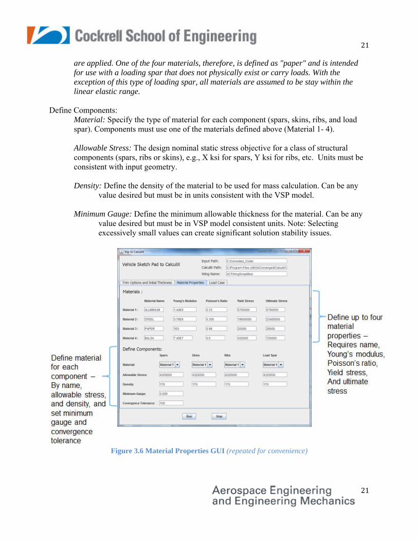
3.6 Material Properties: The materials GUI, shown in Figure 3.6a and repeated in Figure 3.6b, allows input of up to four different kinds of materials. Materials are defined by material name, Young’s Modulus, and Poisson’s Ratio. One of the defined material types is applied to each of four structural component types (skins, spars, ribs, and loading spar). Future VSP SAM releases will include additional material and structural component options.

Figure 3.6 Material Properties GUI Inputs

Materials: Material(1-4): Define up to four different materials. Only the materials defined for the

spars, skins, ribs, and loading spar are necessary; defining additional materials will not impact the run.

Material Name: Input the name of the material to be defined. This name is used when specifying the material used for the spars, skins, ribs, and load spar.

Young’s Modulus: The Young’s Modulus corresponding to the associated material (1-4). Can be any value desired, should be in units consistent with model.

Poisson’s Ratio: The Poisson’s Ratio corresponding to the associated material (1-4). Can be any value desired, should be in units consistent with model.

Yield Stress: The yield stress corresponding to the associated material (1-4). Can be any value desired, should be in units consistent with model.

Ultimate Stress: The ultimate stress corresponding to the associated material (1-4). Can be any value desired, should be in units consistent with model.

Note - As described in Section 2.4, a "loading spar" is defined as a spar in the VSP structural model whether or not a spar is physically located along the line where loads

21

21

are applied. One of the four materials, therefore, is defined as "paper" and is intended for use with a loading spar that does not physically exist or carry loads. With the exception of this type of loading spar, all materials are assumed to be stay within the linear elastic range.

Define Components:

Material: Specify the type of material for each component (spars, skins, ribs, and load spar). Components must use one of the materials defined above (Material 1- 4).

Allowable Stress: The design nominal static stress objective for a class of structural components (spars, ribs or skins), e.g., X ksi for spars, Y ksi for ribs, etc. Units must be consistent with input geometry.

Density: Define the density of the material to be used for mass calculation. Can be any

value desired but must be in units consistent with the VSP model.

Minimum Gauge: Define the minimum allowable thickness for the material. Can be any value desired but must be in VSP model consistent units. Note: Selecting excessively small values can create significant solution stability issues.

Figure 3.6 Material Properties GUI (repeated for convenience)

22

22

3.7 Load Cases and Boundary Conditions: Loads can be applied on the top or bottom surfaces of the wing. Future options will allow simultaneous loads on the top and bottom surfaces as well as other types of loads including inertia and pressure (internal and external)

3.7.1 Five types of design load cases are currently provided. As summarized below, three (3) represent distributed 2-D loads applied along a constant chord fraction line from root to tip. The constant chord line is defined as a loading "spar" and is typically located along a 25% chord line. The 4th type is a set of discrete point loads that can be defined at any number of span and chord fraction locations. The 5th type is for loads applied on or along the front and rear spars at previously trimmed locations.

1. Linear wing load - distributed load varying linearly from wing root to tip 2. Elliptical wing load - theoretical symmetrical elliptical wing load defined by

vehicle weight and load factor. 3. Schrenk’s wing load approximation - Symmetrical elliptical and planform area

averaged running load, also defined by weight and load factor 4. User-defined point loads applied at any number of span and chord fractions.

Loads are defined normal to the surface. 5. Constant distributed loads and/or point loads along a front and/or rear spar are

intended to represent loads from leading and/or trailing edge devices trimmed out (Section 3.4) including loads at the hinge/attachment locations (defined as point forces or moments in any vehicle coordinate direction).

3.7.2 Fixed boundary conditions are applied at user defined inboard rib pairs to approximate wing attach structure as shown in Figure 3.7a. The boundary conditions restrain translation and rotation at the rib pairs.

Fixed Rib Number: The VSP rib number defined as the fixed rib pair.

Figure 3.7a Load Case GUI Inputs – Wing Loading

23

23

3.7.3 GUI inputs associated for the load cases are shown in figures 3.7a, 3.7b, and 3.7c.

Side: Indicates whether the load is applied to the upper or lower wing surface

Figure 3.7a Load Case GUI Inputs – Wing Loading (repeated for convenience)

3.7.4 (Distributed) Wing Loads: Note - See Section 5.0 for wing load methodology

Load Case: Select loading to apply at the loading spar. Choose between: no loading

(NONE), linear load distribution from the root to the tip (LINEAR), elliptical load distribution from the root to the tip (ELLIPTICAL), or Schrenk’s approximation from root to tip (SCHRENK’S).

Load Spar: Input the spar corresponding to the VSP spar number used as the loading spar for the selected load case.

Weight of Aircraft: Gross weight of the aircraft to be used to generate elliptical and Schrenk’s loadings. Use units consistent with other inputs.

Load Factor: Load factor ηz or “g loading” that defines symmetric maneuver load case (i.e. symmetric 2-g pull up corresponds to a load factor of 2).

Root Load: For the linear load case, input the magnitude of the distributed load (in units of force per unit length). Starting at the wing root. The load is applied along a load spar, typically located at the quarter chord. Be sure to use units consistent with the model and other inputs.

Tip Load: For the linear load case, input the magnitude of the distributed load at the tip. Fixed End Moment: An additional external moment can be applied at the wing root (units

of force x length) about the root chord axis independent of the reaction moment. Be sure to use units consistent with the model and other inputs.

24

24

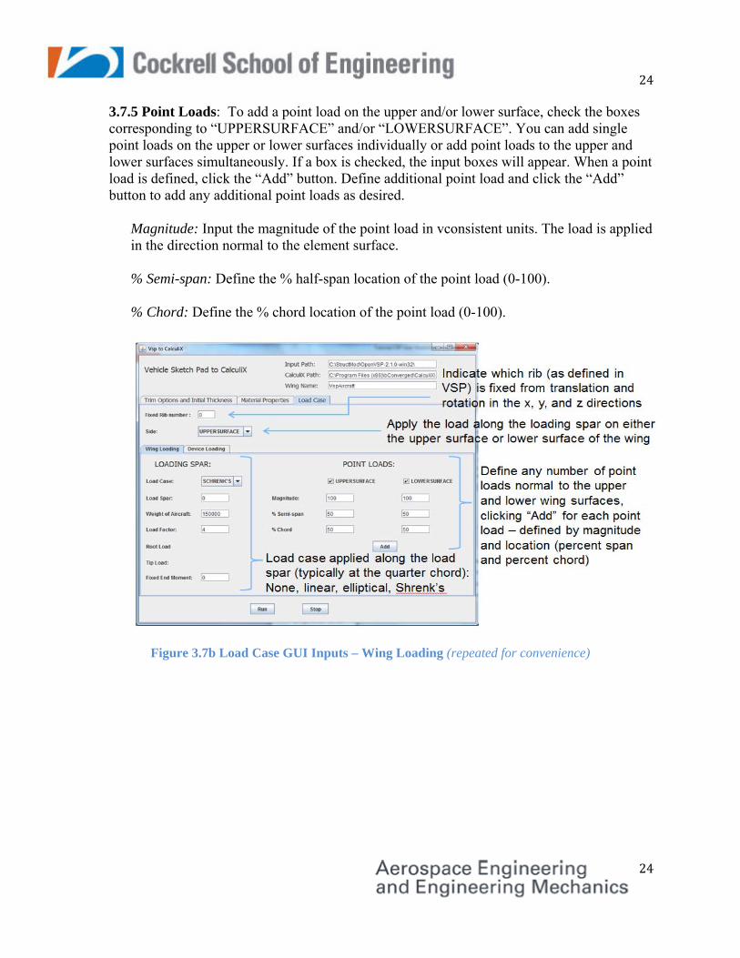
3.7.5 Point Loads: To add a point load on the upper and/or lower surface, check the boxes corresponding to “UPPERSURFACE” and/or “LOWERSURFACE”. You can add single point loads on the upper or lower surfaces individually or add point loads to the upper and lower surfaces simultaneously. If a box is checked, the input boxes will appear. When a point load is defined, click the “Add” button. Define additional point load and click the “Add” button to add any additional point loads as desired.

Magnitude: Input the magnitude of the point load in vconsistent units. The load is applied in the direction normal to the element surface.

% Semi-span: Define the % half-span location of the point load (0-100). % Chord: Define the % chord location of the point load (0-100).

Figure 3.7b Load Case GUI Inputs – Wing Loading (repeated for convenience)

25

25

3.7.6 Device Loads are applied on or along the front and rear spars at previously trimmed locations.

Load Case: Define the load case for each device present. Only devices defined in trim

options will appear. Options include no load (“NONE”), constant distributed load (“LINEAR”), or point loads (“POINT LOADS”).

Linear: Define the magnitude of the constant distributed load, if applicable. Use consistent units.

Point Load: Define the magnitude of the point load, if applicable. When a point load is defined, click the “Add” button. Define an additional point load and click the “Add” button to add any additional point loads as desired. Use consistent units.

% Device Length: Define the % half-span location of the device point load (0-100). Degree of Freedom: Define the direction of the point load. Select between

a force in the x, y, or z direction (Fxx, Fyy, Fzz) or a moment about the x, y, or z axes (Mxx, Myy, Mzz). Apply multiple point loads in different directions at the same point to define a point load in any direction.

Figure 3.7c Load Case GUI Inputs – Device Loading

Note: These inputs are saved as defined in the initial input settings GUI when the “Run” button is pressed. To start a new analysis, click the “Stop” button, and run the software again (See Section 3.2). 3.8 Run CalculiX - Click the Run button. Run times will vary depending on the complexity of the model. Simple models typically run in 1 minute or less

26

26

3.9 Viewing CalculiX Results. When the analysis is complete, the CalculiX post-processor will appear with the finished model and loads/stress/strains available for analysis, as shown in figure 3.8.

a. Put the mouse cursor in the graphic display area, left-click to rotate the model, right click to translate the model, and use the scroll wheel to zoom in and out.

b. To adjust the viewing options, left-click anywhere on the border of the display (i.e. the white part excluding the graphics display). This will bring up a menu with many options, including analysis results labeled as “Datasets”, “Viewing” options, “Animate” options, and the option to select the display “Orientation”.

c. The initial CalculiX display will show the geometry of the analyzed wing only. To return to this view at any point, left-click on the window, select the “Viewing” option in the menu, and choose “Show All Elements With Light”.

d. To view stress distribution, left-click again in the white section, and highlight the “Dataset” option. In this menu, select the “STRESS” option. The menu will close after you click on “STRESS”. Left-click on the background to open the menu again, select “Datasets” again, and highlight the “-Entity-“ option to access the menu for types of stresses to display, including principle stresses, von Mises stresses, and Tresca stresses. We select von Mises stress which is used by VSP SAM to calculate node thicknesses required to meet the user defined design nominal stress objective.

Figure 3.8 A finished CalculiX analysis showing stress results

27

27

e. Using the same method, use the “Datasets” menu to view the displacements (in the x, y, z, or all directions), strains (principle, von Mises, Tresca), and external forces (x, y, z, or all directions). Note - we have found CalculiX issues associated with viewing external force that we have been unable to resolve.

f. Left-click in the background area again, and select the “Viewing” option. The

menu includes the options to: i. “Show All Elements With Light”: View the geometry of the model only.

ii. “Show Bad Elements”: If there is an error in analysis, select this option to view the elements where failure occurred.

iii. “FILL” shows the shaded model iv. “LINES” shows the model as lines corresponding to the boundaries of

elements. This view is useful for viewing internal stress distribution on the ribs and spars.

v. “DOTS” shows the model as dots corresponding to the nodes of the elements.

vi. “Toggle Culing Back/Front”, “Toggle Model Edges”, “Toggle Element Edges”, “Toggle Surfaces/Volumes”, “Toggle Move-Z/Zoom”, and “Toggle Background Color” changes the way in which the model is highlighted and displayed.

vii. “Toggle Vector-Plot”: Plot “needles” to point in the direction of the vectors to display the entity option selected.

viii. “Toggle Add-Displacement”: Visually applies the displacement distribution to see the displacements.

g. Left-click in the background area again and go into the “Animate” menu. Select

“Start” to animate the entity. Animation only works for deflections and external forces.

h. “Frame” is used to adjust the zoom automatically to fit the screen. i. “Zoom” is used to zoom in as an alternative to using the mouse scroll wheel. j. See following section on successfully viewing internal stresses on a CalculiX

model for a description of the “Cut” tool. k. In the menu, select the “Orientation” option to select the view orientation. The

options include “+x view”, “-x view”, “+y view”, “-y view”, “+z view”, and “-z view”. The x, y, and z orientation help view the spars, ribs, and skin surfaces, respectively.

l. See the following CalculiX website for more information on viewing options:

http://www.bconverged.com/calculix/doc/cgx/html/cgx.html

28

28

3.8.1 Viewing CalculiX displayed internal structure

Figure 3.9 CalculiX results display Notation:

LMB = Left-mouse button RMB = Right-mouse button Menu: The menu is accessed by a left click on the “white area” outside the box inside which the wing is being displayed. Then proceed as below:

m. Choose an internal component to visualize (rib, spar, etc) as shown in Figure 3.9. n. Go to : Menu “Orientation” “+z” o. Go to: Menu Viewing Dots. Dots will draw the wing using dots allowing

the user to view internal parts. p. Zoom into and center onto the component you wish to visualize (two mouse

buttons will be required: the RMB and the center scroll wheel). i. Zoom in by pressing down the scrolling wheel, and moving the mouse

upwards (moving the mouse down, i.e. towards the user, zooms out). ii. Press the RMB to translate the model.

q. Go to Menu Cut Node 1 (the element edges will become visible on the model)

i. Once the node is selected, the next mouse click will store it. Be careful not to press any mouse buttons until instructed to do so.

r. Move the cursor to the wing and using LMB select an intersection of the elements (a node) which lies as close to the center of the desired wing component as possible.

s. Go to Menu Cut Node 2

Boxinsidewhichwingisshown

“whitearea”or“backgroundarea”–leftclickingherewillbringupthemenu

Wing

29

29

t. Move the cursor to the wing and using LMB select an intersection of the elements which lies as close to the center of the desired wing component as possible. This must be a node different than the one chosen in step 6.

u. Go to Menu Orientation -z (the model will flip). v. Go to Menu Cut Node 3 w. Move the cursor to the wing and using LMB select an intersection of the elements

which lies as close to the center of the desired wing component as possible. x. Go to Menu Viewing Fill y. Go to Menu Datasets (select the desired data to display and click it). z. Go to Menu Datasets Entity (choose the subset of the data to view) aa. The data is now displayed for the desired component. However, the user may be

required to move the model so that it can be seen. This can be done through the LMB (rotation), RMB (translation), scrolling wheel (zoom), or the orientation option in the menu (see step 2).

3.9 Mass Estimates. When finished viewing the CalculiX output, close the window.

bb. Closing the window will cause the program to go through the mass generation

method and display the mass results based on the initial thickness inputs. cc. Next, VSP SAM will recalculate node thickness required to achieve the desired

input design nominal working stress based on calculated nodal von Mises stress. dd. FEM mass is recalculated again using the design nominal stress based node

thicknesses. The new mass estimate will be displayed as shown in figure 3.10.

Figure 3.10 Mass Estimation Results: Initial (Left) and Calculated (Right)

30

30

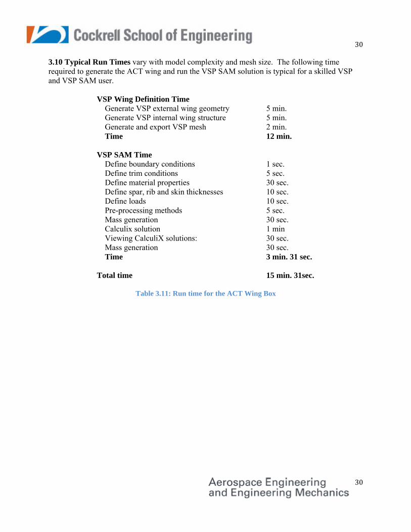
3.10 Typical Run Times vary with model complexity and mesh size. The following time required to generate the ACT wing and run the VSP SAM solution is typical for a skilled VSP and VSP SAM user.

VSP Wing Definition Time Generate VSP external wing geometry 5 min. Generate VSP internal wing structure 5 min. Generate and export VSP mesh 2 min. Time 12 min. VSP SAM Time Define boundary conditions 1 sec. Define trim conditions 5 sec. Define material properties 30 sec. Define spar, rib and skin thicknesses 10 sec. Define loads 10 sec. Pre-processing methods 5 sec. Mass generation 30 sec. Calculix solution 1 min Viewing CalculiX solutions: 30 sec. Mass generation 30 sec. Time 3 min. 31 sec. Total time 15 min. 31sec.

Table 3.11: Run time for the ACT Wing Box

31

31

4.0 VSP SAM Issues and Cautions 4.1 Overall. The following is a list of currently known issues and cautions for VSP SAM users:

1. Running excessively large ( > 5 Mb) VSP mesh files significantly increases run time and in some cases will cause a memory allocation failure when running CalculiX. Simplification of the model or a larger mesh will be required to fix the problem.

2. VSP SAM must be run in VSP consistent units (i.e. if the VSP model is defined in feet,

then all inputs must be in feet to include material properties and allowables). 3. Wing trim is restricted to defined spar and rib locations. For a trim to take place, a

leading edge and/or trailing edge spar must exist and ribs located at span-wise trim locations must exist, unless the entire leading edge/trailing edge is trimmed.

4. Trimming of leading and trailing edge devices is limited to two devices each along the leading edge and trailing edges.

5. A paper spar may be defined for the loading spar if the user wishes to apply a line load where a spar does not physically exist.

6. Up to four materials may be defined by the user and applied to four structural component types (spars, ribs, skins, and loading spar). Future releases may have a larger material library to include orthotropic and composite materials.

7. Point loads on the upper and lower surfaces of the wing can be defined only in the

direction normal to the element surface as a load across an entire element. Along the trim devices, however, the point loads can be applied to elements as forces in the x, y, or z direction or moments in the x, y, or z direction. Future releases will accommodate applied forces in x,y,z directions along spars and ribs.

4.2 Structural Sizing Methodology Limitations Users are cautioned that the practical result of the static FEM stress based sizing methodology developed for VSP SAM is a highly idealized structural representation of a wing or empennage component. The FEM model makes no allowance for fasteners, damage tolerance, fatigue or other "real world" effects. In its current form, the model also does not address buckling; although, we have an initiative under way to do so. Sizing is also based on a single load case, which is another issue that will be addressed by future releases. In essence, the sizing methodology generates a purely static stress based, idealized structure that requires application of a significant design nominal stress "knock down" to account for factors not included. Research currently underway at UT will provide quantitative guidance on recommended knock down factors. In the meantime, users are advised to limit application of the methodology to trade studies that are performed around well-developed structural baseline representations.

32

32

Other limitations in the current methodology include:

Above the elastic range of the material, the stresses calculated by the FEM analysis are invalid and local yielding will occur to redistribute the internal loads. Our current thickness methodology analysis does not make allowance for abnormally high localized stresses. A refined methodology is under development and will be described in future releases of VSP SAM. The current thickness sizing methodology is based on a single sizing iteration and represents a non-converged stress solution since stress changes will result from redistribution of internal loads. An iterative method is currently under development and will be described in future releases of VSP SAM. Multiple design load case analysis is required to size realistic structure. Load cases are typically not additive and require multiple sequential load case analyses for sizing. Methodology for multiple load case analysis is under development. Rib-rib and spar-spar defined bays are not sized for buckling. Methodology is under development to include buckling in the sizing methodology.

33

33

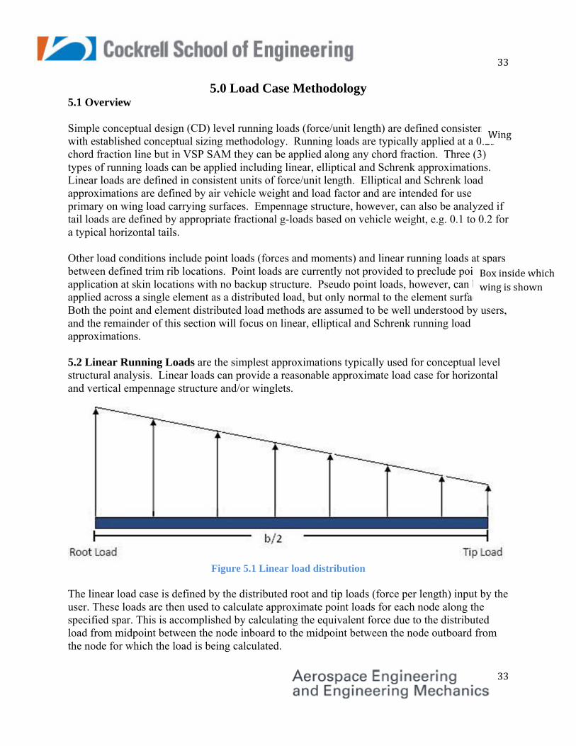
5.0 Load Case Methodology 5.1 Overview Simple conceptual design (CD) level running loads (force/unit length) are defined consistent with established conceptual sizing methodology. Running loads are typically applied at a 0.25 chord fraction line but in VSP SAM they can be applied along any chord fraction. Three (3) types of running loads can be applied including linear, elliptical and Schrenk approximations. Linear loads are defined in consistent units of force/unit length. Elliptical and Schrenk load approximations are defined by air vehicle weight and load factor and are intended for use primary on wing load carrying surfaces. Empennage structure, however, can also be analyzed if tail loads are defined by appropriate fractional g-loads based on vehicle weight, e.g. 0.1 to 0.2 for a typical horizontal tails. Other load conditions include point loads (forces and moments) and linear running loads at spars between defined trim rib locations. Point loads are currently not provided to preclude point load application at skin locations with no backup structure. Pseudo point loads, however, can be applied across a single element as a distributed load, but only normal to the element surface. Both the point and element distributed load methods are assumed to be well understood by users, and the remainder of this section will focus on linear, elliptical and Schrenk running load approximations. 5.2 Linear Running Loads are the simplest approximations typically used for conceptual level structural analysis. Linear loads can provide a reasonable approximate load case for horizontal and vertical empennage structure and/or winglets.

Figure 5.1 Linear load distribution

The linear load case is defined by the distributed root and tip loads (force per length) input by the user. These loads are then used to calculate approximate point loads for each node along the specified spar. This is accomplished by calculating the equivalent force due to the distributed load from midpoint between the node inboard to the midpoint between the node outboard from the node for which the load is being calculated.

Boxinsidewhichwingisshown

Wing

34

34

5.3 Elliptical Loading Approximation. Elliptical load approximations are standard practice for conceptual-level modeling of static wing loads at a defined normal load factor (nz). The load is typically applied along the wing quarter chord, but it is not required in VSP SAM (any constant chord line can be defined). The magnitude of the elliptical load is calculated from aircraft weight and load factor as described below. Loads are converted to equivalent forces at defined node locations and averaged across adjacent elements.

Figure 5.2 Elliptical load distribution

VSP wing models are defined in symmetrical left and right hand pairs, and Figure 5.2 shows a half-span representation with an elliptical running load, where the maximum is at the root and goes to zero at the tip. For a given air vehicle of gross weight (w) at a constant defined load factor ( ) he equation for an elliptical distribution for the semi-span is given as

2 ∙ ∙

∙ 2

1

2

where is the distributed load (force per length) is the total wing span (length)

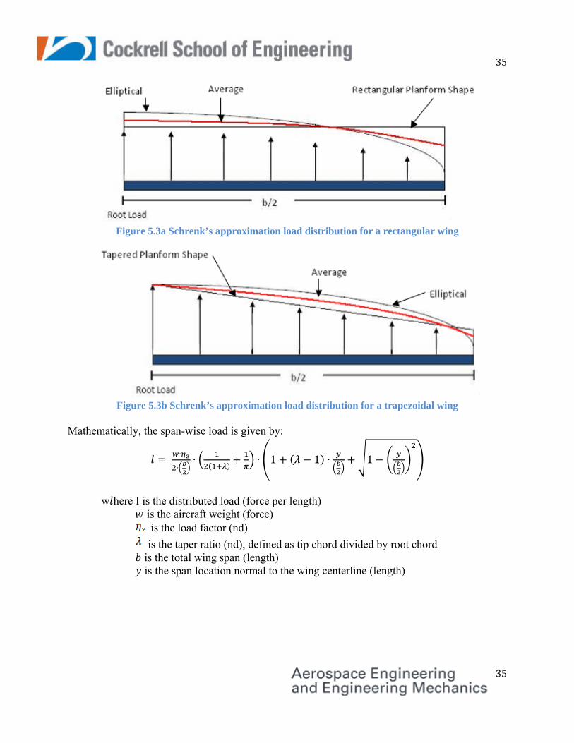
is span location (length) From the defined elliptical distribution, point loads are calculated for each node along the specified spar. The running load is converted to equivalent forces acting on nodes. 5.4 Schrenk’s Approximation is a semi-empirical span-wise load distribution for non-elliptical wing planforms. The method assumes the load distribution is equivalent to the average of the elliptical load distribution and the actual planform shape distribution of the wing. The method requires calculation of the average of the chord variation and the elliptical load variation at a defined span location, as shown in Figures 5.3 below, for rectangular and trapezoidal planforms. Similar to elliptical load distributions, Schrenk loads are typically applied along the quarter chord line, but it is not a VSP SAM requirement.

35

35

Figure 5.3a Schrenk’s approximation load distribution for a rectangular wing

Figure 5.3b Schrenk’s approximation load distribution for a trapezoidal wing

Mathematically, the span-wise load is given by:

∙

∙∙ ∙ 1 1 ∙ 1

w here I is the distributed load (force per length) is the aircraft weight (force) is the load factor (nd)

is the taper ratio (nd), defined as tip chord divided by root chord is the total wing span (length) is the span location normal to the wing centerline (length)

36

36

6.0 Thickness Sizing Methodology 6.1 Overview A simple static stress-based structural thickness methodology is used to size FEM components to achieve an overall input design nominal stress level across the model. Thickness sizing is based on FEM calculated nodal von Mises stress. The method is applied to node, instead of element, thickness to avoid thickness discontinuities between elements. Design nominal stress objectives are currently input for three (3) classes of structural components (spars, ribs and skins). Minimum gage thickness constraints are also defined. The current version of VSP SAM does one thickness sizing iteration at the end of a single CalculiX stress solution. Future versions will iterate solutions to convergence. The current sizing methodology produces a highly-idealized static stress sized model suitable for structural trade studies. If used for point design analysis, users are cautioned to use significant design nominal stress knock-down factors to account for real-world design considerations not currently included in the methodology. 6.2 Node Thickness Sizing Methodology VSP FEM methodology sizes the FEM model to achieve a constant overall design nominal stress level across the structure. The VSP SAM FEM model is based on shell elements of fixed grid size where, by definition, structural components are one (1) element thick. Stress sizing, therefore, reduces to a single design variable, thickness. The stress sizing method compares the FEM calculated von Mises stress at each node to the input design nominal working stress objective and recalculates node thickness to achieve the desired stress level. Thickness required to achieve a desired stress level at any element node of known thickness (t1) for an arbitrary 3D element is defined by the ratio of the calculated stress (1) to a desired node stress objective (obj). The basis for the relationship is shown in Figure 5.1 and is derived below:

Figure 5.1 3D element with a plane on a principal stress axis

The blue plane represents a plane lying in one of the 3 principal stress axes, showing that the element can be arbitrarily oriented. The stress acting on the plane, which has a defined area and length (L), is defined by the relationship:

∙

Thickness 

37

37

Since element length is defined by input mesh size and the force is defined for the node, we see that 1 1/t1 or 1 t1 = constant and the thickness (t1) associated with a given stress (1) is related to any other stress and thickness combination (2, t2) by

∙ ∙ Therefore, node thickness required to achieve a design nominal stress objective σ σ

is given by ∙

The thickness relationship is valid anywhere within the elastic range of the material. At low stress levels, however, node thickness will be defined my material minimum gage, which is another required material property input. 6.3 Thickness Methodology Limitations Users are cautioned that the practical result of the static FEM stress based sizing methodology described above is a highly idealized structural representation of an airframe component. The FEM model makes no allowance for fasteners, damage tolerance, fatigue or other "real world" effects. In its current form it also does not address buckling; although, we have an initiative under way to do so. Sizing is also based on a single load case, which is another issue that will be addressed by future releases. So in essence, the sizing methodology generates a purely static stress based, idealized structure that requires application of a significant design nominal stress "knock down" factors to account for factors not included. Research currently underway at UT will provide quantitative guidance on recommended knock down factors. In the meantime, users are advised to limit application of the methodology to trade studies that are performed around well-developed structural baseline representations. Other limitations in the current methodology include:

Above the elastic range of the material, the stresses calculated by the FEM analysis are not valid and local yielding will occur to redistribute the internal loads. Our current thickness methodology analysis does not make allowance for abnormally high, localized stresses. A refined methodology is under development and will be described in future releases of VSP SAM. The current thickness sizing methodology is based on a single sizing iteration and represents a non-converged stress solution since thickness changes will result in a redistribution of internal loads. An iterative method is currently under development and will be described in future releases of VSP SAM. Multiple design load case analysis is required to size realistic structure. The load cases are typically not additive and require multiple sequential load case analyses sizing. Methodology for multiple load case analysis is under development. Rib-rib and spar-spar defined bays are not sized for buckling. Methodology is under development to include buckling in the sizing methodology.

38

38

7.0 Mass Estimation Methodology 6.1 Overview

VSP SAM estimates structural mass from finite element model (FEM) volume and input material density. Spar, rib and skin FEM volumes are calculated separately based on the sum of the mesh elements for each part component class. Element volume is defined by the thickness of the nodes that define each element. Node thickness is calculated as described in Section 5. 6.2 Element Volume The VSP generated mesh, as input to VSP SAM, is a zero-thickness surface to which a user input thickness distribution is applied across nodes. The starting FEM mass, therefore, is a little more than a calculated value that reflects user defined estimates of node thickness required to react internal loads (stresses) or to meet deflection requirements. After the first von Mises stress calculation, node thickness required to meet input defined nominal stress objectives are calculated and the volume of the resulting FEM model will represent the amount of material required to meet structural requirements. FEM mesh elements can be either triangular or trapezoidal shape, as defined by VSP. From the VSP defined shape, the area of each element can be calculated using standard method for any arbitrary triangle or rectangle given by:

, , , , , , , ,

where and are the position vectors between two points using x, y, and z coordinates. From these areas, the volume is calculating by multiplying the element area by the average thickness for the element. Using the user-defined material densities from the inputs, the masses are then generated.

∗3

∗4

∙

39

39

8.0 Appendix

8.1 Verification of CalculiX Results: A VSP wing is generated with a rectangular airfoil and analyzed as a rectangular cross-section beam. Thewingisanalyzedasacantileverrectangularbeamloadedalongthe50%chordlineandfixedattherootrib.

The cross sectional geometry is shown below.

Figure 8.1 Rectangular Cross-Section Beam with geometric definitions

The stress results generated by CalculiX are shown below.

Figure 8.2 Top view of beam with stress results in CalculiX

0.05 ,

2.0

0.25

10

40

40

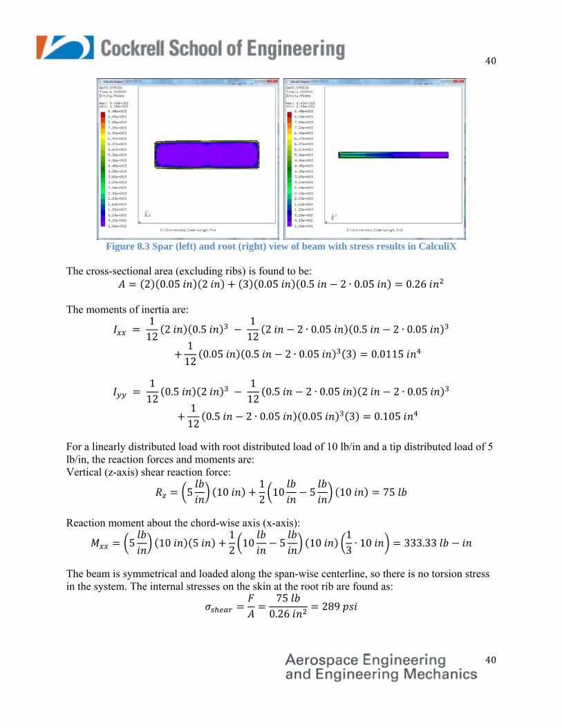
Figure 8.3 Spar (left) and root (right) view of beam with stress results in CalculiX

The cross-sectional area (excluding ribs) is found to be:

2 0.05 2 3 0.05 0.5 2 ∙ 0.05 0.26 The moments of inertia are:

112

2 0.5 112

2 2 ∙ 0.05 0.5 2 ∙ 0.05

112

0.05 0.5 2 ∙ 0.05 3 0.0115

112

0.5 2 112

0.5 2 ∙ 0.05 2 2 ∙ 0.05

112

0.5 2 ∙ 0.05 0.05 3 0.105

For a linearly distributed load with root distributed load of 10 lb/in and a tip distributed load of 5 lb/in, the reaction forces and moments are: Vertical (z-axis) shear reaction force:

5 101210 5 10 75

Reaction moment about the chord-wise axis (x-axis):

5 10 51210 5 10

13∙ 10 333.33

The beam is symmetrical and loaded along the span-wise centerline, so there is no torsion stress in the system. The internal stresses on the skin at the root rib are found as:

750.26

289

41

41

, ,

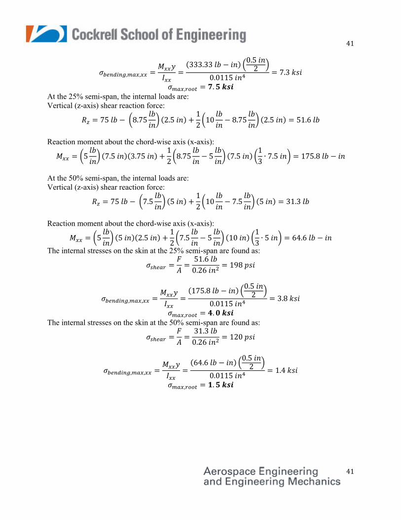
333.33 0.52

0.01157.3

, . At the 25% semi-span, the internal loads are: Vertical (z-axis) shear reaction force:

75 8.75 2.51210 8.75 2.5 51.6

Reaction moment about the chord-wise axis (x-axis):

5 7.5 3.75128.75 5 7.5

13∙ 7.5 175.8

At the 50% semi-span, the internal loads are: Vertical (z-axis) shear reaction force:

75 7.5 51210 7.5 5 31.3

Reaction moment about the chord-wise axis (x-axis):

5 5 2.5127.5 5 10

13∙ 5 64.6

The internal stresses on the skin at the 25% semi-span are found as: 51.60.26

198

, ,

175.8 0.52

0.01153.8

, . The internal stresses on the skin at the 50% semi-span are found as:

31.30.26

120

, ,

64.6 0.52

0.01151.4

, .

42

42

8.3 Verification of mass generation results: The volume is calculated as

2 3 10 0.05 3 0.3 10 0.055 3 0.3 0.05 3.68

The material is defined as aluminum, so the density of the material is 0.1 . The mass of

the beam is then found to be

3.68 0.1 0.368

Figure 8.4 Mass generation results from the VSP to CalculiX software