Embed Size (px)
Citation preview

Confronting climate change: Adaptation vs. migration strategies in
Small Island Developing States
Lesly Cassin, Paolo Melindi Ghidi, Fabien
Prieur
WP 2020.09
Suggested citation: L. Cassin, P. Melindi Ghidi, F. Prieur (2020). Confronting climate change: Adaptation vs. migration strategies in Small Island Developing States. FAERE Working Paper, 2020.09.
ISSN number: 2274-5556
www.faere.fr

Confronting climate change: Adaptation vs.migration strategies in Small Island Developing States
Lesly Cassin∗ Paolo Melindi Ghidi † Fabien Prieur‡
Abstract
This paper examines the optimal adaptation policy of Small Island Developing
States (SIDS) to cope with climate change. We build a dynamic optimization prob-
lem to incorporate the following ingredients: (i) local production uses labor and
natural capital, which is degraded as a result of climate change; (ii) governments
have two main policy options: control migration and/or conventional adaptation
measures ; (iii) migration decisions drive changes in the population size; (iv) expa-
triates send remittances back home. We show that the optimal policy depends on
the interplay between the two policy instruments that can be either complements or
substitutes depending on the individual characteristics and initial conditions. Using
a numerical analysis based on the calibration of the model for different SIDS, we
identify that only large islands use the two tools from the beginning, while for the
smaller countries, there is a substitution between migration and conventional adap-
tion at the initial period.
Keywords: SIDS, climate change, adaptation, migration, natural capital.
JEL classification: Q54, Q56, F22.
∗EconomiX, University Paris Nanterre; 200, Avenue de la République 92000, Nanterre, France. E-mail:[email protected].†EconomiX, University Paris Nanterre & AMSE, Aix-Marseille University, e-mail:
[email protected].‡CEE-M, University of Montpellier, CNRS, INRAE, Montpellier SupAgro, Montpellier, France. Email:
1

1 Introduction
Climate change affects regions all around the world. The effects of climate change onindividual regions are heterogeneous and depend on the ability of different societal andenvironmental systems to respond to it. Two main (policy) responses are commonly putforward: mitigation and adaptation. Mitigation consists in limiting the extent of thechange by reducing greenhouse gas emissions. Adaptation refers to all the measures –investment in protective infrastructure, management of endangered ecosystems, changesin production and consumption habits, etc. – intended to absorb the impact of climatechange. In general, a combination of these two strategies seems warranted in order toaddress the climate issue in the most efficient way. But there is no one-fits-all solution:the best mix between adaptation and mitigation significantly differs across regions becauseof their heterogeneity.
The case of Small Island Developing States (SIDS) is emblematic of the inability torest on these two pillars. This can be explained by their two unique characteristics.First, SIDS are not responsible for the ongoing increase in temperatures and have nomeans to stamp it out on their own. Second, they are among the most vulnerable to itsrepercussions.1 This implies that SIDS have no other option but to rely on adaptationmeasures. According to the Intergovernmental Panel on Climate Change (IPCC), climatechange damages for these countries will be so large that adaptation is a necessary conditionfor a sustainable economic development (see for instance UN-OHRLLS (2017)).2
In this paper, we focus on the situation of SIDS and consider a third possible strategyto cope with climate change: migration, as a specific form of adaptation. If migration is adirect consequence of the worsening of living conditions due to climate change, then thisprocess should be accompanied and eased by the design of appropriate public policies.
1Indeed SIDS will face an increase in the occurrence of extreme weather events (more frequent andsevere storms and hurricanes, etc.), a rise in sea level accompanied by the degradation of natural capital,and health problems including infectious diseases (Nurse et al. (2014), Klöck and Nunn (2019)).
2http://unohrlls.org/custom-content/uploads/2017/09/SIDS-In-Numbers_Updated-Climate-Change-Edition-2017.pdf
2

In other words, we want to adopt the perspective of a policy maker in SIDS who triesto figure out how to turn climate migration, which would otherwise be the last resortoption, into a deliberate long term policy. The basic cost-benefit analysis is as follows.Climate-induced migration is, of course, disruptive on many grounds, as any form ofmigration. Nevertheless, in the context of SIDS, it also comes with benefits. On theone hand, migration is a means to release the pressure on scarce natural resources. Onthe other, migration will likely trigger financial transfers directed toward the SIDS, asmigrants provide financial support to their family, in the form of remittances.
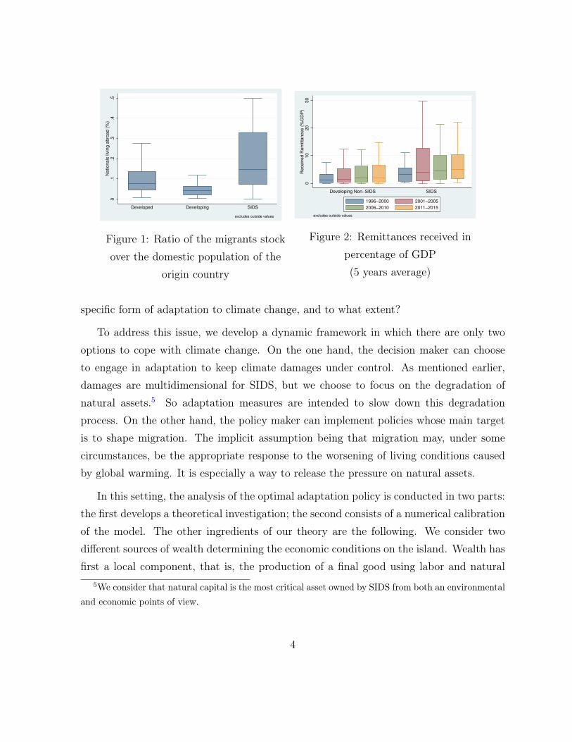
There is a tradition of studying the impact of climate change on migration (see amongothers Barrios et al. (2006), Marchiori and Schumacher (2011), Gray and Mueller (2012);Marchiori et al. (2012), Thiede et al. (2016)). We depart from this literature since ourapproach is normative, by construction. It is motivated by two observations. First, gov-ernments in SIDS are already considering migration as a credible adaptation strategy.For example, the “Migration with dignity” program by the Kiribati government aims atincreasing investments in public education and schooling in order to make Kiribati mi-grants more attractive to receiving countries.3 Moreover, international organizations suchas the World Bank, the United Nations and more specifically the International Orga-nization for Migration (IOM), present migration as an explicit tool to foster economicdevelopment. Here the emphasis is on the financial role of migration that endows origincountries with additional resources thanks to remittances (Agunias and Newland (2012),Clemens (2017)).4 Second, migration is an important dimension of the demography ofSIDS, that shapes their economic performance. For instance, Figure 1 displays the longterm average–between 2000-2015–of the share of nationals living abroad by region. Fig-ure 2 depicts the evolution of remittances in the percentage of GDP in SIDS and otherdeveloping countries. Both figures show that migration is massive and that it generatesrelevant economic returns for these developing islands.
Based on these observations, our main research question is: What is the optimaladaptation policy for SIDS? A corollary question being: Should they use migration as a
3http://www.climate.gov.ki/category/action/relocation/.4http://publications.iom.int/system/files/pdf/mecc_outlook.pdf.
3
0.1
.2.3
.4.5
Nation
als
liv
ing
ab
road
(%
)
Developed Developing SIDS
excludes outside values
Figure 1: Ratio of the migrants stockover the domestic population of the
origin country
010
20
30
Re
ce
ive
d R
em
itta
nces (
%G
DP
)
Developing Non−SIDS SIDS
excludes outside values
1996−2000 2001−2005
2006−2010 2011−2015
Figure 2: Remittances received inpercentage of GDP(5 years average)
specific form of adaptation to climate change, and to what extent?
To address this issue, we develop a dynamic framework in which there are only twooptions to cope with climate change. On the one hand, the decision maker can chooseto engage in adaptation to keep climate damages under control. As mentioned earlier,damages are multidimensional for SIDS, but we choose to focus on the degradation ofnatural assets.5 So adaptation measures are intended to slow down this degradationprocess. On the other hand, the policy maker can implement policies whose main targetis to shape migration. The implicit assumption being that migration may, under somecircumstances, be the appropriate response to the worsening of living conditions causedby global warming. It is especially a way to release the pressure on natural assets.
In this setting, the analysis of the optimal adaptation policy is conducted in two parts:the first develops a theoretical investigation; the second consists of a numerical calibrationof the model. The other ingredients of our theory are the following. We consider twodifferent sources of wealth determining the economic conditions on the island. Wealth hasfirst a local component, that is, the production of a final good using labor and natural
5We consider that natural capital is the most critical asset owned by SIDS from both an environmentaland economic points of view.
4

capital. An active migration policy induces a contraction of the output thanks to theassociated decrease in the labor force. However, as the local population decreases, thepopulation of emigrants increases, which is associated with more remittances receivedfrom abroad. This yields the second external source of wealth. In line with the evidenceprovided earlier, remittances are large enough to involve a real economic trade-off in themanagement of the population. Overall, migration affects welfare both directly (cf. thetotal utility criterion), and indirectly by changing the amount of per capita consumption.As far as adaptation is concerned, there is a direct cost of adaptation in terms of foregoneconsumption. At the same time, the benefit stems from the capacity to maintain thestock of natural capital to a higher level and for a more extended time.
The analysis of the intertemporal decision problem is quite challenging because itgenerically produces a four-dimension dynamical system and can exhibit four differentregimes, depending on whether the two instruments, migration and adaptation, are oper-ative or not. To circumvent these difficulties, we first have a look at regimes in which thepolicy relies on one instrument only, and then combine our main findings to understandwhat is going on in the regime where both instruments are used. Considering first aregime with no adaptation, the SIDS suffers from the impacts of climate change and hasno option but to adjust its population size. We find a critical condition on the funda-mentals of the economy under which there exist migration incentives at the beginning ofthe planning period. In this situation, the optimal migration policy is characterized bya monotonically decreasing emigration rate, that vanishes eventually when the optimalpopulation size is reached. When there is no migration incentive initially, but the SIDSbears an increasing environmental constraint because of climate change, we identify acondition that tells us if a switch to a positive migration regime will occur in finite time.
Next, we study a regime with no migration along the same line. In the absence ofmigration, the only possibility left is to undertake adaptation expenditures. We then findanother critical condition, that also involves most of the economy’s fundamental, underwhich the SIDS starts to adapt from the origin. When the regime with positive adaptationis permanent, during the convergence to the saddle point, adaptation expenditures de-
5

crease monotonically over time but remain positive, which in turn ensures that the SIDSwill enjoy a higher level of natural capital in the long run. Finally, merging both analyses,we conduct a formal discussion on the features of the optimal policy in general terms.When there is no adaptation initially but positive migration, the incentives to switch onthe second instrument increase over time as the decrease in the population size reducesthe marginal cost of adaptation. In the symmetric situation where there is adaptationbut no migration initially, we highlight the condition that triggers a switch to positivemigration in finite time. Moreover, if the regime with positive adaptation and migrationhosts a steady state, then we show that the SIDS manages to stabilize natural assets to aconstant and higher level than in the absence of adaptation. As a result, the populationsize is also larger in the long run.
To sum up, from the theoretical investigation, we obtain two critical conditions thatshed some light on the SIDS preferred policy to deal with climate change. Using aspecification of the model, we discuss which instrument the SIDS will deploy in priority tomanage the damages optimally due to global warming, and how this choice depends on thecritical parameters. To dig further into the analysis of the nature of the optimal policy, wefinally resort to a calibration of the model to real-world data. This calibration is a meansto emphasize the role of the initial conditions, that is, the initial size of the populationand the initial endowment in natural capital. More importantly, this exercise ultimatelyhelps us to understand which policy is optimal for which SIDS, given its characteristics.Last but not least, it allows us to explain when adaptation and migration, both seen aspolicy instruments, prove to be complements or substitutes.
The paper is organized as follows. In Section 2 we briefly review the literature onclimate change damages and migration. Section 3 displays the model, which is thenanalyzed in Section 4. Section 5 is devoted to the calibration, while Section 6 concludes.
6

2 Related Literature
SIDS show a strong heterogeneity politically, economically, socially or culturally, however,according to the IPCC they face common constraints in terms of vulnerability and adap-tation to climate change (Nurse et al., 2014). First of all, due to their high density ofpopulation, even spatially limited degradations may impact a large share of the popula-tion. Second, while the topology of these islands vary a lot according to their location ortheir geological formation, they all show a high concentration of their economic activitieson the coastal areas. Finally, the weight of the natural assets in their economies is morelikely to be high compared to other developing states. This is due to their specializationin tourism or fisheries (Nurse et al., 2014). Therefore, even if the various climate changerisks do not affect the different SIDS in the same way, they all exhibit a high vulnerabilityto them. In order to cope with those risks, adaption is crucial. Klöck and Nunn (2019)propose a literature review on SIDS adaptation to climate change. Most of the articlesdescribed in this paper focus on a region, an island or a sector and show that adaptationefforts were inefficient (Dey et al., 2016b,a; Rosegrant et al., 2016; Valmonte-Santos et al.,2016; Weng et al., 2015; Mercer et al., 2012; Middelbeek et al., 2014; Vergara et al., 2015).Moreover, more general studies such as those of Scobie (2016) and Thomas and Benjamin,2018 also find that the adaptation strategies in the SIDS are far from sufficient and thatthey lack of coherence. All in all, this seems to be accounted for by the technical andfinance limits.
Besides conventional adaptation investments, migration seems to be a very plausiblesolution for small countries. Theoretical works such as Marchiori and Schumacher (2011),show that human displacements increase if no mitigation strategies are implemented bylarge emitters of GHG. According to this result, empirical papers try to predict the evo-lution of migration with climate change. They base their work on the past variations inhuman deplacements according to environmental factors such as the rainfall variability,the precipitations volume or the temperature. Among others, Nawrotzki et al. (2015) pre-dicts a climate-induced increase in the international out-migration from Mexico. Thiedeet al. (2016) find that depending on the region, migration is correlated to climate vari-
7

ability for eight South-American countries. Moreover, papers as Marchiori et al. (2012)or Barrios et al. (2006) find a positive correlation between weather anomalies or climatechange and migration in Sub-Saharan countries. Farbotko and Lazrus (2012), predicts aclimate induced increase in the out-migration from Tuvalu, a Pacific island.
In all those papers, however, the effects of environmental degradations on economicoutcomes and investments are neglected. Consequently, these works fail to take into ac-count both optimization strategies to cope with climate change and the trade-off betweenadaptation and migration in order to adapt. On the contrary, Lilleor and den Broeck(2011) introduce the interaction between climate change and economic outcomes high-lighting the demographic response to this interaction. They find a positive correlationbetween the loss of revenue due to climate change and migration, but no effects from theincome variability due to the increasing weather variability.
A third group of papers explicitly introduces economic gains from migration for thesending economies. First, migration is a means to reduce the demographic pressure onthe environment (Birk and Rasmussen (2014)). Second, migration could enhance invest-ments in adaptation, especially in protective infrastructures, because remittances can helpfinance adaptation measures (Ng’ang’a et al. (2016)). In the same vein, Julca and Pad-dison (2010) concludes that migration and remittances are valuable levers for the SIDSeconomies. However, on the downside, the authors stress the dependence from remittancesas a potential growing issue.6 More generally, in these papers migration and adaptationare seen as complements. Nevertheless, there is a bunch of papers that support the oppo-site view by observing that when migration is (already) very high, the need for adaptationactions is less urgent (see for instance Barnett and Adger (2003)). Embracing this ar-gument boils down to considering migration and adaptation as substitutes. In any case,since the 1990s, the management of the diaspora strategy by the originating country ispresented as a new policy tool that has been studied in the political geography literature.De Haas (2010) emphasizes that migration based on individual decisions could be ineffi-
6Hugo (2011) take a more nuanced position by claiming that sending areas might experiment manydifferent economic, demographic and social adjustments that are difficult to anticipate.
8

cient. In this view, increases in the migration gains could be obtained thanks to publictransnational policies based on the coordination (and the cooperation) with the diaspora(Faist (2008), De Haas (2010), Agunias and Newland (2012), Mullings (2012)). While allthese papers are not directly in line with our approach, they acknowledge the existenceof tools to shape migration. Of course, these tools are more relevant in the context ofcountries experiencing large scale migration like the SIDS.
In this paper, we depart from those three branches of the literature by developing anormative approach on migration as an alternative strategy to cope with climate change.The novelty of our work is to highlight both the potential complementarity and substi-tutability between migration and conventional adaptation strategies.
3 Model
We consider an infinite horizon SIDS economy and adopt a centralized perspective. Timeis continuous and indexed by t ∈ [0,∞). Assuming away demographic growth, any changein the population size, N(t), is the result of migration, with m(t) = 0 the emigration level:
N(t) = −m(t). (1)
The emigration rate simultaneously determines the evolution of the population ofexpatriates, M(t):
M(t) = m(t). (2)
Three main ingredients are needed to characterize the SIDS: the definition of its wel-fare, the composition of its wealth, and the impacts of climate change.
Social welfare of the SIDS, V (c(t),m(t)N(t)), is made of two components. The firstis total utility, N(t)U(c(t)), where c(t) represents per capita consumption and U(.) isincreasing and concave. The second is the cost of migration, D(m(t)), withD(.) increasingand strictly convex. If migration becomes a deliberate strategy to deal with climatechange, then the decision maker should take into account the costs borne by those who
9

embark on the resettlement process. These costs are typically linked to the culturaldifferences, travel distance, and immigration policy in the destination country.7 Puttingtogether these two elements, we get:
V (c(t),m(t), N(t)) = N(t)U(c(t))−D(m(t)). (3)
Two comments are in order here. First, according to this formulation, the plannercares about the local inhabitants while migrants no longer matter once their resettlementprocess is completed. The planner’s priority is to deal with the local situation that de-teriorates thanks to the impacts of climate change. In this context, migration representsa form of long term adaptation. In other words, it is a specific instrument among thetools available to solve the problem. This characteristic prevails over the socio-economicdimension of migration (that encompasses the situation of migrants as individuals). Inthe literature review, we emphasized that international organizations present migrationas a tool to foster economic development. This is not very different from the perspectivewe adopt here. Second, the question of how society should allocate its resources when thepopulation is not constant is an old and important one. In welfare economics, utilitar-ianism allows to address this issue. In the utilitarian theory, there exist two conflictingapproaches. According to the Benthamite view, society should care about the total utilityof the members of the society. This is in contrast to the Millian perspective accordingto which this is the average utility, not the total utility, that matters. Neither classicalnor average utilitarianism provides a satisfactory answer to the issue of how to choose thepopulation size optimally.8 And both have their advocates and opponents.
Our purpose is not to enter this debate, though quite thrilling. The reason why wechoose to use the classical version is the following. Let C be aggregate consumption.Other things equal, the average utility U(C
N) is decreasing in N whereas if we take the
7Defining D(.) more generally in terms of m and M(t) would allow us to also account for the socialdamage from migration in the origin country whose origin is the loss of social interactions, culturaltransmission and family links that come with migration. This is left for future research.
8Under fairly general conditions, they have implications that are ethically unacceptable, see Razinand Sadka, 2001, and references therein.
10

derivative of the total utility NU(CN
) w.r.t N , we get:
∂NU(CN
)
∂N= U
(C
N
)(1− σu) with σu =
CNU ′(C
N)
U(CN
).
Assuming that σu < 1, we get that total utility is increasing in N . Coming back toour motivation, given that we want to study migration driven by environmental (andfinancial) motives, it seems quite natural and logical to neutralize the other drivers ofmigration (and population change), and in particular the one related to the way societyvalues the population size. Unlike average utilitarianism, classical utilitarianism allowsus to do that since in the absence of remittances and climate change, the SIDS economywould not be willing to experience a decrease in the population thanks to migration.
Wealth in the SIDS, W (K(t), N(t)), has two origins. It locally produces a uniquefinal good, Y (t), by means of a constant returns to scale technology using natural capital,K(t), and labor, N(t): Y (t) = F (K(t), N(t)), with Fi > 0, Fii < 0 for i = K,N , andFKN > 0. What is worth noticing at this stage is that production capacities are limited bythe amount of available natural assets, this is referred to as the environmental constraint.This constraint is expected to be increasing across time, as the negative repercussionsof climate change will materialize. The SIDS also receives remittances, R(M(t)), fromabroad. They are supposed to be increasing and concave with respect to this population.
Combining (1)-(2), we get a direct connection between the two populations: M(t) =
N0 +M0−N(t) for all t, with N0 > 0 andM0 ≥ 0 the initial population size of respectivelyinsular people and the diaspora. This allows us to express total wealth as follows:
W (K(t), N(t)) = F (K(t), N(t)) +R(N0 +M0 −N(t)). (4)
Under fairly general conditions, the wealth function is either monotone increasing inN , or inverted U-shaped, for K positive and given.9 We consider the latter case. Denoteby N∗(K) the wealth maximizing population size, for K given. At the initial condition,we impose that
9Take its first derive w.r.t. N : WN (K,N) = FN (K,N)−R′(N0−N). Assuming limN→0 FN (K,N) =
∞ > R′(N0 + M0), W is either always increasing in N on (0, N0), or ∃!N∗(K) ∈ (0, N0) /WN (K,N∗(K)) = 0, with N∗′(K) > 0.
11

Assumption 1 N0 > N∗(K0)⇔ WN(K0, N0) < 0. This is also equivalent to FN(K0, N0) <
R′(M0).
This condition means that at the beginning of the planning program, the combinationof the environmental constraint and the opportunity to resort the external funding of theeconomy through remittances is such that there exist incentives to undertake positivemigration. This does not mean however that SIDS necessarily finds it optimal to go forpositive migration from the origin because Assumption 1 only captures wealth motives,whereas migration is also accompanied by welfare effects. Since, everything else beingequal, welfare is increasing in N , the SIDS has no incentive to decrease its populationsize. In other words, Assumption 1 provides a necessary condition for a regime withpositive migration.
This assumption seems to be the most appropriate, especially if one wants to describethe optimal migration policy (even) in the absence of climate damage.10 A glance athistory shows us that the SIDS display a long tradition of migration, whose fundamentalcauses are partly environmental but not linked to climate change. We by no way claim thatthe migration flows that have been observed in these islands for decades can be attributedto any sort of optimal policy. Still, historical evidence suggests that positive migrationmay have been optimal for some SIDS. The key factor here is not the initial populationsize but the endowment of natural capital per capita. Thus we find it reasonable to givean account of the heterogeneity of SIDS, and resulting differences in migration patterns,which is what Assumption 1 allows.
Climate impacts show themselves in the degradation of the stock of natural asset, ata constant rate δ > 0. Natural capital typically refers to the amount of arable lands,freshwater reserves, the endowment of the SIDS in marine and terrestrial ecosystems etc.To preserve these natural assets, the SIDS can by no way rely on mitigation since it hasno capacity to affect the pattern of worldwide emissions on its own. Besides migration,the only option left to cope with climate change is then to invest in adaptation measures.For simplicity, we model adaptation as a decision variable, s(t) ≥ 0, which suitably
10This corresponds to the case in which K0 is constant.
12

captures adaptation expenditures in ecosystems maintenance for instance.11 Adaptationis a means to slow down the ongoing process of deterioration of K(t). It however comesat an increasing and strictly convex cost, G(s(t)). Defining as ε(s(t)) the returns onadaptation, ε(.) being decreasing and convex with ε(0) = 1, the law of motion of K(t) isgiven by:
K(t) = −δε(s(t))K(t) + δK∞. (5)
Absent any climate change, K(t) would remain constant and equal to K0. Under ongoingclimate change but without public adaptation, K(t) decreases exponentially at rate δ,going asymptotically to a strictly positive, though potentially very low, value K∞.
Before summarizing the decision problem, it is worth formulating a general remarkregarding our approach. In the literature review, we emphasized that the emigration pol-icy has been considered as a tool for economic development for a long time. Moreover,we provided support for the perspective we adopt in this work, that consists in consid-ering migration as an extreme form of adaptation. This of course supposes that decisionmakers can affect migration decisions and flows through targeted public policies.12 Thatbeing said, rather than modeling explicitly the education sector or interactions with theexpatriates population and how they relate to migration, we make a shortcut by assumingthat the decision maker directly chooses the number of emigrants, m(t).13
In the end, the intertemporal decision problem can be written as follows:
max{s(t),m(t)}
∫ ∞t=0
V (c(t),m(t), N(t))e−ρtdt, (6)
11Therefore, by construction, our model is not designed to account for investments in adaptationinfrastructure such as sea walls and dikes.
12Policies that seem particularly relevant are the ones that deal with education and the managementof the diaspora.
13The assumption is made for simplicity and conveys the idea that governments in SIDS can ultimatelycontrol the decision to migrate. This is admittedly an oversimplified description of the real world. Wehowever believe that this is the appropriate way to address the problem, especially because our aim isto study the optimal adaptation policy for SIDS. The alternative approach would have gone through theexplicit modeling of individual migration decisions and their links with relevant public policies. This isan interesting extension of the current research that is left for future work.
13

with ρ > 0 the rate of pure time preference, subject to the resource constraint, c(t) =W (K(t),N(t))−G(s(t))
N(t), (1), (3), (4), and (5). Consumption is strictly positive whereas we
have to account for the non-negativity constraints on m(t) and s(t). Finally, for theproblem to be meaningful, we must focus on the situation where K(t) ≤ 0, i.e., there isno man-made natural capital. This would normally require to add another constraint tothe optimization. For simplicity, we do not explicitly incorporate this constraint. But wewill take care of it in the coming analysis.
4 Optimal policy
The optimization program above is a two-state two-control variable control problem.Taking into account the non-negativity constraints, the Lagrangian is:14
L = NU
(W (K,N)−G(s)
N
)−D(m)− λNm+ λK(−δε(s)K + δK∞) + µmm+ µss,
with λN and λK the co-state variables associated with N and K, and µm, µs ≥ 0 theLagrange multipliers for m and s.
Denote the elasticity of utility with respect to consumption and the elasticity of con-sumption with respect to N respectively by σu and σc:
σu =cU ′(c)
U(c)and σc(N ;K, s) = −NcN
c,
where the elasticity σu is assumed to be constant with σu ∈ (0, 1).
The set of (necessary) optimality conditions is given by:
D′(m) + λN ≥ 0, m(D′(m) + λN) = 0
G′(s)U ′(c(N,K, s)) + ε′(s)δλKK ≥ 0, s(G′(s)U ′(c(N,K, s)) + ε′(s)δλKK) = 0
λN = ρλN − U(c(N,K, s)) (1− σc(N ;K, s)σu)
λK = (ρ+ δε(s))λK − FK(K,N)U ′(c(N,K, s))
N = −mK = δ(K∞ − ε(s)K)
(7)
14The time index is omitted when there is no danger of confusion.
14

where c(N,K, s) is the compact notation for the consumption function.
The first condition in (7) is related to the choice ofm, and we immediately observe thatλN must be negative for experiencing a regime with m > 0. We come back to this point ina moment. The second optimality condition refers to the adaptation strategy. Adaptationinvolves the following trade-off. A marginal increase in adaptation expenditures is a meansto slow down the deterioration of natural capital, a benefit that is measured at its socialvalue. However, such an increase also implies that the economy has less resources availablefor consumption, this cost being measured in (marginal) utility terms
Overall the optimality conditions in (7) define a four-dimension dynamical systemthat may encompass four regimes depending on whether m, s = 0. This kind of systemis hardly manageable in general due to the dimensionality and non-linearity problems.Our aim in the following analysis is to get as much insight from the theoretical analysisas possible. For that purpose, we choose to work with projections in plans composed ofa state variable and its corresponding control – or co-state – variable, taking the othervariables as given. With the support of graphical illustrations, this should allow us toaddress the following questions: which regime can arise along the optimal solution? Whatare the dynamic features of these regimes? Is it possible for the economy to experiencea switch from one regime to the other? We ultimately want to identify some criticalconditions that may help us to understand which policy, in terms of the combination andtiming of implementation of the two instruments, is optimal for which SIDS, based on itscharacteristics.
4.1 Insights from the theoretical analysis
We start with the analysis of a regime with no adaptation, s = 0, which means thatthe SIDS incurs the impacts of climate change and has no other option but to designits migration policy optimally in order to adapt to them. All proofs are gathered in theAppendix.
15

4.1.1 Regime with no adaptation
We first study the dynamics of population and migration when assuming that s = 0.Then we look at the joint evolution of the stock of natural capital and its shadow value.
The migration decision comes with a direct (marginal) cost, captured by D′(m), andpotential benefits through the adjustment of the population size, that are captured bythe shadow value of N . Consider the interior solution first (m > 0, µm = 0). Combiningthe first condition in (7) with the one characterizing the dynamics of the shadow valueλN yields the following dynamic system in the (N,m) plan: m = mσ−1
d
(ρ+ U(c(N,K(t),0))
D′(m)(1− σuσc(N ;K(t), 0))
),
N = −m.
with σd = mD′′(m)D′(m)
> 0 the elasticity of the marginal damage, also assumed constant, andK(t) = (K0 −K∞)e−δt +K∞.
Take K as given, and for the ease of discussion, equal to K0. This means that thereis no impact of climate change on the SIDS. In this situation, it is relatively easy to showthat the condition
σuσc(N0, K0, 0) > 1 (8)
is necessary and sufficient to get a permanent regime with m(t) > 0 for t < ∞ (see theAppendix A.1.1). This condition involves both wealth and welfare effects. Wealth effectsare captured by the elasticity σc(N0;K0) since σc(N0;K0) = 1 + σw(N0;K0) and σw isthe elasticity of wealth w.r.t the population size. They have been discussed in detailfollowing Assumption 1 that states that there exist migration incentives (as far as wealthis concerned). Welfare effects have to do with σu. The size of σu, which belongs to (0, 1),tells us about how strongly society is affected by a change in the population size. Indeed,remember that ∂NU(C
N)
∂N= U
(CN
)(1−σu) > 0. Now the inequality above indicates that the
optimal policy features positive migration when the wealth benefit from migration (andthe decrease in the population size) exceeds the welfare costs associated with it. Notethat this is most likely to be true when σu is close to one, which means that society barelyfeels the impact of the decrease in population (as ∂NU(C
N)
∂Nis close to zero in this case).
16

Under condition (8), it cannot be optimal to switch to m = 0 in finite time. Startingfrom a positive level of migration, migration flows decrease monotonically. The migrationprocess ends up eventually when the population size approaches its steady state valueN(K0), that solves σuσc(N,K0, 0) = 1.
Considering the exogenous degradation of K makes the dynamic analysis a bit morecomplex but does not change the main conclusion (see the Appendix A.1.2). Logically,and still assuming that condition (8) holds, as the burden imposed by the environmentalconstraint gets stronger and so is the dependence on remittances, the incentives to under-take positive migration are higher at any instant. The optimal migration policy displaysthe same qualitative features as the one depicted earlier. In the long run, natural capitalconverges to its degraded stationary value, K∞. This in turn means that the populationsize has to decrease further in order to adapt to the much lower level of natural capi-tal available to the SIDS. It will stabilize in the long run to the level N(K∞) such thatσc(N(K∞);K∞, 0) = σ−1
u . See Figure 3 for an illustration.
When σc(N0;K0, 0) < σ−1u , there is no migration incentive originally. Considering a
constant K, we would get a trivial stationary solution with no population change. Herehowever considering the degradation of the stock of natural capital (because of climatechange) may lead to a different conclusion. Indeed, provided that the initial emigrationratio is low enough,
M0
N0
<σr(M0)
σ−1u − 1
(9)
with σr(M) = MR′(M)R(M)
> 0 the elasticity of remittances w.r.t. the stock of expatriates,15
there exists a (unique) critical stock of natural capital such that it becomes optimal toinitiate the migration process: let K(N0) be this stock, which solves σc(N0;K, 0) = σ−1
u .Therefore a switch to migration will occur in finite time if and only if K∞ < K(N0). Theintuition of this result is quite simple. Under climate change, the environmental constraintincurred by the SIDS may become so high that at some point it is optimal to undertakepositive migration in order to release the pressure imposed on natural assets. From that
15This elasticity is equal to one – and the RHS of (9) does not depend on M0 – when remittances areproportional to the size of the diaspora, R(M) = rM , a specification that will be used later.
17

date on, migration follows an inverted-U shaped trajectory until the convergence to thesame steady state. See Figure 4 for an illustration.
Figure 3: Positive migration always
m
N·N = 0N(K0) N0N(K∞)
·m = 0 |K=K∞
·m = 0 |K=K0
Figure 4: From m = 0 to m > 0
m
N·N = 0N(K∞)
H(N; K∞)
N0H(N; K0)
H(N; K(N0))
Let us now examine what is going on in the (K,λK) plan. In this regime, the dynamicsare simply given by: {
λK = (ρ+ δ)λK − FK(K,N)U ′(c(K,N, 0))
K = δ(K∞ −K)
Replacing s = 0 in the second condition in (7) and assuming that it holds with anequality, we can characterize the critical geometric locus that divides the (K,λK) into twodomains, the one with s = 0 and the one with s > 0: λK = ξ(K;N), with ξK(K;N) < 0
and s = 0 when λK < ξ(K;N).
Working first with N given, the locus λK = 0 defines another relationship between λKand K, which is parameterized by N : λK = ζ(K;N), with ζK(K;N) < 0, and λK > 0 forλK > ζK(K;N). Then we immediately obtain that the regime with no adaptation expen-diture hosts a unique steady state with K∞ = K∞ and λK∞(N) =
FK(K∞,N)U ′(c(K∞,N))
ρ+δ.
During the convergence to the steady state, as the stock of natural capital deteriorates,its shadow value increases monotonically (see Figure 5 and the Appendix A.1.3).
Starting from the initial condition (N0, K0), such a trajectory is feasible if and only ifthe domain where s = 0 and λK > 0 is non-empty. Defining K(N0) as the unique solution
18

to ξ(K;N0) = ζK(K;N0), this boils down to imposing:
K(N0) > K0. (10)
This condition captures the initial trade-off embodied in the choice of going for adap-tation, or not. It basically compares the marginal benefit from the first unit of adaptationwith its marginal cost.
Considering the decrease in population size resulting from an active migration policy,things get more complicated. The two critical loci ξ(K;N) and ζ(K;N) move down,which results in an increase in K(N), and it proves difficult to assess the feasibility of apath featuring s = 0 for all t. One can however observe that as N decreases the regionof the (K,λK) plan in which it is optimal not to adapt shrinks. This also comes as nosurprise. Other things equal, with the decrease in N , the SIDS incentives to undertakes get bigger as the opportunity cost of adaptation, in terms of foregone consumption,becomes lower.16 This means that we cannot in general rule out the occurrence of aregime change from s = 0 to s > 0. As a rough illustration, Figure 6 depicts the optimaltrajectory, in red, obtained for N constant and equal to N0. With N decreasing and thefrontiers moving down, it is possible that by following such a trajectory, the SIDS lies inthe domain associated with s > 0 at a finite point in time and starts adapting to climatechange thanks to this specific instrument.
We now turn to the analysis of the regime with positive adaptation.
4.1.2 Regime with positive adaptation
For the sake of simplicity, we continue the ongoing analysis by making use of specificfunctional forms: U(c) = σ−1
u cσu , σu ∈ (0, 1); D(m) = 11+σd
m1+σd , σd ≥ 1; Y = AKαN1−α,A > 0, α ∈ (0, 1); R(M) = rM , r > 0; G(s) = γs, γ > 1; and ε(s) = e−ηs, η > 0. Fortechnical elements, refer to the Appendix A.2.
16Indeed, per capita consumption increases and marginal consumption increases when N decreases.
19

Figure 5: Regime s = 0, N0 constant
λK
K
( ·K = 0)
ζ(K; N0)
K∞
ξ(K; N0)
K0 K(N0)
s>0
s=0
Figure 6: Regime s = 0, N decreasing
λK
K
( ·K = 0)
ζ(K; N0)
K∞
ξ(K; N0)
K0 K(N )K(N0)
ξ(K; N )ζ(K; N )
Using these specifications, we can define:
Φ(K;N) =η
γαAKαN1−α − 1,
and express the dynamical system as follows:{λK = [ρ− δε(s)Φ(K;N)]λK
K = δ(K∞ − ε(s)K)
Let us work with N constant, and equal to N0 first. Noticing that the critical levelK(N0), defined just before, is also the solution to Φ(K;N0) = ρ
δ, the condition
K(N0) < K0 (11)
is necessary and sufficient for the existence of a well-behaved regime with positive adap-tation expenditures. If we further impose:{
K(N0) < K∞,
Φ(K0;N0) < ρδK0
K∞,
(12)
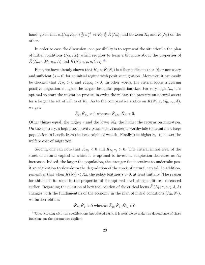
then there exists a unique steady state parameterized by N0, (K∞(N0), s∞(N0)), withK∞(N0) ∈ [K∞, K0], K ′∞(N) > 0 and s′∞(N) > 0. During the transition to the steadystate, the natural capital decreases monotonically and so do adaptation expenditures. We
20
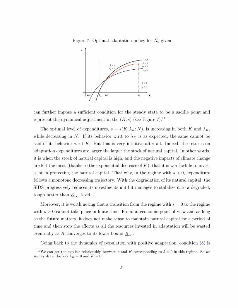
Figure 7: Optimal adaptation policy for N0 given
s
KK(N ) K∞ K(N ) K0
·K > 0·K < 0
·K < 0
·λK > 0·λK > 0
·λK < 0
φ(K )
ϵ(K; N )
can further impose a sufficient condition for the steady state to be a saddle point andrepresent the dynamical adjustment in the (K, s) (see Figure 7).17
The optimal level of expenditures, s = s(K,λK ;N), is increasing in both K and λK ,while decreasing in N . If its behavior w.r.t to λK is as expected, the same cannot besaid of its behavior w.r.t K. But this is very intuitive after all. Indeed, the returns onadaptation expenditures are larger the larger the stock of natural capital. In other words,it is when the stock of natural capital is high, and the negative impacts of climate changeare felt the most (thanks to the exponential decrease of K), that it is worthwhile to investa lot in protecting the natural capital. That why, in the regime with s > 0, expenditurefollows a monotone decreasing trajectory. With the degradation of its natural capital, theSIDS progressively reduces its investments until it manages to stabilize it to a degraded,tough better than K∞, level.
Moreover, it is worth noting that a transition from the regime with s = 0 to the regimewith s > 0 cannot take place in finite time. From an economic point of view and as longas the future matters, it does not make sense to maintain natural capital for a period oftime and then stop the efforts as all the resources invested in adaptation will be wastedeventually as K converges to its lower bound K∞.
Going back to the dynamics of population with positive adaptation, condition (8) is17We can get the explicit relationship between s and K corresponding to s = 0 in this regime. So we
simply draw the loci λK = 0 and K = 0.
21

no longer necessary to have positive migration. Besides the usual wealth and welfareeffects associated with migration, devoting a positive amount of resources to adaptationgives higher incentives to adjust the population size to get the highest possible income.In such a context, we expect that the dynamics in the (N,m) remain similar to what weget in Section 4.1.1. In particular, as long as the SIDS starts with positive migration, theemigration rate should vanish only asymptotically.
The reverse inequality, σc(N0;K0, 0) < σ−1u , is now necessary (but not sufficient) for a
regime with m = 0 together with s > 0 to take place initially. In this case, it is relativelyeasy to provide a necessary and sufficient condition for a switch to m > 0 in finite time:
σc(N0;K∞(N0), s∞(N0)) > σ−1u (> σc(N0;K0, 0)). (13)
A last remark can be formulated. It is difficult to go further in the study of the dynamicbehavior of the SIDS when located in the regime with positive adaptation and positive –but asymptotically going to zero – migration. A complete analysis would especially requireto deal carefully with the issue of existence of a steady state for the general system (7).Rather, we simply want to make the following observation, assuming that a steady stateexists. When the SIDS economy devotes resources to adaptation, it manages to maintainthe stock of natural capital to a level above the lowest bound K∞, which is compatiblewith a larger population size than in the absence of such expenditures. Not surprisingly,monitoring the speed at which natural capital deteriorates and managing to stabilize itslevel in the long run ultimately provides the SIDS economy with more latitude for ensuringa good enough standard of living for a larger number of inhabitants.
4.2 Discussion
Let us now put together all the pieces of information we get so far. As far as the optimalpolicy is concerned, our analysis reveals that the SIDS has two qualitatively differentoptions to cope with the negative repercussions of climate change. Interestingly, twoconditions on the fundamentals of the economy help to explain which policy is optimal inwhich context. These conditions involve the ranking between K0 and K(N0) on the one
22
hand, given that σc(N0;K0, 0) R σ−1u ⇔ K0 Q K(N0), and between K0 and K(N0) on the
other.
In order to ease the discussion, one possibility is to represent the situation in the planof initial conditions (N0, K0), which requires to learn a bit more about the properties ofK(N0; r,M0, σu, A) and K(N0; γ, ρ, η, δ, A).18
First, we have already shown that K0 < K(N0) is either sufficient (s > 0) or necessaryand sufficient (s = 0) for an initial regime with positive migration. Moreover, it can easilybe checked that KN0 > 0 and KN0N0 > 0. In other words, the critical locus triggeringpositive migration is higher the larger the initial population size. For very high N0, it isoptimal to start the migration process in order the release the pressure on natural assetsfor a larger the set of values of K0. As to the comparative statics on K(N0; r,M0, σu, A),we get:
Kr, Kσu > 0 whereas KM0 , KA < 0.
Other things equal, the higher r and the lower M0, the higher the returns on migration.On the contrary, a high productivity parameter A makes it worthwhile to maintain a largepopulation to benefit from the local origin of wealth. Finally, the higher σu, the lower thewelfare cost of migration.
Second, one can note that KN0 < 0 and KN0N0 > 0. The critical initial level of thestock of natural capital at which it is optimal to invest in adaptation decreases as N0
increases. Indeed, the larger the population, the stronger the incentives to undertake pos-itive adaptation to slow down the degradation of the stock of natural capital. In addition,remember that when K(N0) < K0, the policy features s > 0, at least initially. The reasonfor this finds its roots in the properties of the optimal level of expenditures, discussedearlier. Regarding the question of how the location of the critical locus K(N0; γ, ρ, η, δ, A)
changes with the fundamentals of the economy in the plan of initial conditions (K0, N0),we further obtain:
Kγ, Kρ > 0 whereas Kη, Kδ, KA < 0.
18Once working with the specifications introduced early, it is possible to make the dependence of thesefunctions on the parameters explicit.
23

So, we can conclude that the larger γ and/or the lower A, the higher the cost of theadaptation policy. In the same vein, the lower η, the lower the returns on adaptationexpenditures. Finally, when ρ is high, people attach less value to what happens in thelong run, while a low δ means that climate change translates into a slow degradation ofthe natural capital. This all points to the fact that the set of initial conditions for whichit is optimal to choose s = 0 expands.
Overall, we can conclude that there exist two main policy alternatives for the SIDS.Either the SIDS implements – at least initially and possibly permanently – a policy relyingon only one of the two instruments, which makes them substitutes. Or the SIDS adoptsa policy combining adaptation and migration from the origin, the two instruments beingcomplements. Figure 8 provides a representation of the different possible combinations ofthe two instruments in the special case where M0 = 0.19 For a large enough N0 (largerthan the intersection between K(N0) and K(N0)), we see that there are three possibilitiesdepending on the initial endowment in natural capital. For a large enough K0, it isoptimal to go for adaptation first, while not using the migration tool. Migration maybecome operative at some later date, depending on whether condition (13) is met. Quiteon the contrary, for K0 low enough, there is no point at spending resources in adaptationand the only option left is migration. Finally in intermediate situations, the optimalpolicy consists of a mix between adaptation and migration right from the beginning.
Figure 8: Different optimal policies in the (N0, K0) plan
N0
K0
K(N0)
K(N0)
s ≧ 0, m > 0
s > 0, m ≧ 0
s, m > 0s ≧ 0, m ≧ 0
19In this case, condition (9) is always fulfilled.
24

5 Calibration
In this section, we bring the model to the data in order to complement the theoreticalanalysis presented in the previous section. We calibrate the different parameters as well asthe initial conditions for the main variables. In the coming exercise, a particular emphasiswill be placed on international comparisons.
5.1 Parameters calibration
Among the parameters some values common to all the SIDS are taken from the economicliterature or computed. In the theoretical analysis, we assume that the cost of infrastruc-ture expenditure is linear: G(s) = γs, with γ > 1. The parameter γ can be interpretedas the marginal cost of public funds. To our knowledge, there is no paper providing anestimation of γ for SIDS countries. We therefore use a value in line with the estimationscalculated by Auriol and Warlters (2012) using a sample of African countries, that isγ = 1.2.20 The share of labor in production–i.e. parameter (1 − α) in our model–is notthe same in all countries. Therefore, we consider the average of values for SIDS given inthe Pennsylvania World Table (PWT) (Feenstra et al. (2015)), (1− α) = 0.55.21
The choice of the value of ρ, the rate of pure time preference, has led to an intensedebate in the literature (Tol (2006), Nordhaus (2007), Dasgupta (2008)). We use 0.04,but we have performed the numerical analysis for values ranging between 0.04 and 0.2to be consistent with the literature (see Appendix A.4 for the robustness checks). Forthe sake of simplicity, we choose a quadratic function for the marginal cost of migration,which implies that σd = 1. As for the utility function, we take σu = 0.95, which meansthat we work with a function that displays features close to a linear one. We implement
20Note that the results are not very sensitive to the value of γ, when varying between 1 and 2. Thisclaim has been tested in the supplementary comparative statics analysis provided in Appendix A.4.
21Another solution would be to evaluate the value of α accordingly to the natural capital stock valueswhich are retained. However, in this case, the calibration of the rest of the model, especially for remit-tances function, would be less accurate. The robustness tests for the calibration with different definitionsof natural capital stock are available upon request.
25

robustness tests for σu = {0.9; 0.95; 0.99}.22 The other parameters are determined usingthe following method:
• The total factor productivity (TFP): A
The value of the Total Factor Productivity (TFP), A, is calibrated on data fromthe PWT and the World Development Indicators (WDI). We compute the Cobb-Douglas function of the model using the following data from the PWT: population,country level labor share and output stock in Purchasing Power Parity (PPP). More-over, we define the natural capital stock as the sum of the value added from tourismas well as agriculture, forestry and fisheries (AFF) in the World Development Indi-cators (WDI).23 Note that tourism is incorporated in order to capture the economicgains from landscapes on these islands. We apply the standard growth accountingframework to our production function. According to it, economic growth can bedecomposed into contributions from inputs, here labor and natural capital. There-fore, in order to obtain annual growth rate of the TFP for country i, we computethe following equations:
giTFP = gioutput − (1− α)gilabor − αgicapitalTFPi = 1 + giTFP
where the growth rate of the variable x is defined as: gx = (x(t + 1) − x(t))/x(t).We use long-term average for SIDS, which is 1.01. Note that we conduct robustnesstests on the value of the TFP according to the minimum and the maximum valuecomputed for the SIDS, which are respectively 0.96 and 1.08 (cf. Appendix A.4).
• Initial Values22Robustness results are given in the Appendix A.4.23We have also conducted a calibration where the natural capital is defined as the sum of the capital
stock from the PWT and the value added from tourism and the AFF. For developing countries the lattermethodology gives output that are less correlated to the GDP than the retained method, while for SIDS,the results remain the same (cf. Appendix A.4).
26

We define the diaspora size as the average of the emigrant stock between 2000 and2015, using the data-set of the United Nations, Department of Economic and SocialAffairs, Population Division (POP/MIG). However, in order to have a better com-parison between countries as well as to respect the scale of the model, we divide thevalues from the different dataset by 106 to get the initial conditions for population(Ni0), the stock of natural capital (Ki0) and the stock of migrants (Mi0).
• The remittances coefficient: r
Next we want to compute the value of r, given the linear specification used: R(M(t)) =
rM(t). A preliminary step is to compute the level of remittances perceived in theeconomy. The total amount received from the diaspora is obtained using the vari-able “remittances perceived in percentage of GDP” from the WDI data-set, thisvariable is denoted by Ri(t) in our calibration. First, we calibrate the value of theremittances, Ri(t), according to the following equation:
Yi(t) = TFPi(t)×Ki(t)α ×Ni(t)
1−α
Ri(t) = Ri(t)× Yi(t)
Then, we regress Ri(t) on the computed values of the diaspora size to get the valueof r. The value of this coefficient for the SIDS is reported in Table 1.24 Note thatthe results displayed in the table tend to support our choice for the definition ofnatural capital. Indeed, the coefficient of correlation between the migrants stockand the remittances perceived is higher if capital is computed as the sum of theAFF and tourism added values than with the alternative definition.
Table 2 summarizes the parameters values used to calibrate the model.25 Table 3gives the long term average values retained for the local population, the diaspora and the
24This calibration works quite well for islands, with a R2 = 0.72, while the correlation is not as goodfor other developing countries or developed countries, for the reasons explained above.
25The values retained for σu, γ, δ, η, and ρ are in bold print, while the other computations are givenin A.4.
27
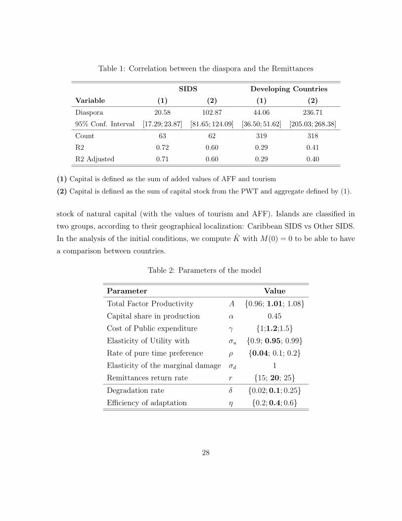
Table 1: Correlation between the diaspora and the Remittances
SIDS Developing Countries
Variable (1) (2) (1) (2)
Diaspora 20.58 102.87 44.06 236.71
95% Conf. Interval [17.29; 23.87] [81.65; 124.09] [36.50; 51.62] [205.03; 268.38]
Count 63 62 319 318
R2 0.72 0.60 0.29 0.41
R2 Adjusted 0.71 0.60 0.29 0.40
(1) Capital is defined as the sum of added values of AFF and tourism
(2) Capital is defined as the sum of capital stock from the PWT and aggregate defined by (1).
stock of natural capital (with the values of tourism and AFF). Islands are classified intwo groups, according to their geographical localization: Caribbean SIDS vs Other SIDS.In the analysis of the initial conditions, we compute K with M(0) = 0 to be able to havea comparison between countries.
Table 2: Parameters of the model
Parameter Value
Total Factor Productivity A {0.96; 1.01; 1.08}Capital share in production α 0.45Cost of Public expenditure γ {1;1.2;1.5}Elasticity of Utility with σu {0.9; 0.95; 0.99}Rate of pure time preference ρ {0.04; 0.1; 0.2}Elasticity of the marginal damage σd 1Remittances return rate r {15; 20; 25}
Degradation rate δ {0.02;0.1; 0.25}Efficiency of adaptation η {0.2;0.4; 0.6}
28

Table 3: Initial Conditions
Countriesa Populationb Mig. Stockc AFFd Tourisme Nat. cap.f
Other SIDS
COM 653,547.13 97,925.75 471,785,696 54,433,940 526,219,648
CPV 487,067.75 145,873.25 224,986,560 553,566,592 778,553,152
FJI 844,610.19 168,499 684,939,776 1,424,057,600 2,108,997,376
GNB 1,480,094 90,425 890,059,712 30,794,654 920,854,336
MDV 344,131.75 2,139.75 240,465,408 2,589,127,936 2,829,593,344
MUS 1,231,074.25 141,176.75 770,540,736 2,943,838,464 3,714,379,264
STP 165,723.25 30,233 45,970,536 34,740,660 80,711,200
SYC 89,187.75 10,377.75 45,081,308 633,793,280 678,874,560
Caribbean SIDS
ABW 99,813 13,666.75 15,343,271 1,876,686,592 1,892,029,824
ATG 91,951.88 57,153.75 30,930,550 612,512,640 643,443,200
BHS 344,067.44 35,616.25 116,810,920 2,218,210,560 2,335,021,568
BLZ 302,807.06 53,181.25 298,639,648 438,550,592 737,190,272
BRB 276,888.25 94,207 67,785,448 1,050,887,680 1,118,673,152
CUW 145,550.55 65,692.75 13,903,565 938,107,072 952,010,624
DMA 71,116.94 63,148.5 79,620,696 131,192,264 210,812,960
DOM 9,560,993 1,083,748.25 6,067,153,920 9,270,968,320 15,338,122,240
GRD 103,934 63,629.5 56,855,876 219,942,768 276,798,656
HTI 9,631,816 1,009,448 3,009,077,248 716,374,976 3,725,452,288
JAM 2,776,172.25 940,470.75 1,257,011,456 3,692,628,992 4,949,640,192
LCA 167,849.06 47,970.75 60,580,300 574,474,560 635,054,848
SUR 512,644.13 248,161.25 575,558,464 162,111,264 737,669,760
TTO 1,312,901.5 330,561.5 218,717,136 1,186,257,792 1,404,974,976
VCT 108,885.81 56,054.25 62,329,152 182,764,736 245,093,888
aLegend: COM: Comoros, CPV: Cabo Verde, FJI: Fiji, GNB: Guinea-Bissau, MDV: Maldives,MUS: Mauritius, STP: Sao Tome and Principe, SYC: Seychelles, ABW: Aruba, ATG: Antigua andBarbuda, BHS: Bahamas, The, BLZ: Belize, BRB: Barbados, CUW: Curacao, DMA: Dominica,DOM: Dominican Republic, GRD: Grenada, HTI: Haiti, JAM: Jamaica, LCA: Saint-Lucia, SUR:Suriname, TTO: Trinidad and Tobago, VCT: Saint-Vincent and the Grenadines
bSource: PWTcMigrant Stock, source: UNSDdSoure: WDI. Value added, PPP 2011$eSource: WDI. International receipt, PPP 2011$fSum of AFF and Tourism
29

5.2 Results
The first objective of our numerical analysis is to understand the position of each SIDSin the plan of the initial conditions and thus to answer to the following question: whatis the optimal strategy of each island to cope with climate change? Figure 9 displays,in logarithmic scale plots, the position of each island according to their initial values forcapital and population. We also represent on the same plan the two critical loci, K(N)
and K(N), derived in the theoretical analysis, that are given by the following equations:
K(N0) =
(γ(ρ+ δ)
δηA(1− σF )Nα−1
0
) 1α
, (14)
K(N0) =
(rNα−1
0 (N0 −M0(σ−1u − 1))
A(σ−1u − α)
) 1α
. (15)
Note that these two curves are drawn by assuming that SIDS share what we call thecommon parameters, i.e., all the parameters except the initial conditions. We choose tofocus on the heterogeneity with respect to the initial conditions because of the insightsgiven by theoretical investigation. In particular, it has been emphasized that they arecrucial to understand SIDS potential development path in a world with climate change.
Remind that if a country is located above the curve K, optimal migration can be nil,while if it is below the curve, it will always be positive. Moreover, if the country positionis below the curve K, investments in adaptation measures can be zero, while if it is abovethe curve there will be positive adaptation expenditures.
Several remarks arise from the observation of Figure 9. First of all, there exists acritical threshold for the population size, 1.5 million inhabitants, that determines whetherit is optimal to systematically go for adaptation. When the population is larger than thisthreshold, the optimal policy is based on adaptation, that may be complemented withmigration. On the contrary, if the population is very small, the island is likely locatedbelow the curve of K. In this scenario, using adaptation measures is optimal only forcountries with very large stock of natural. For example, Barbados and the Bahamas areabove the curve K because of their large endowment in natural capital. Indeed, their
30

amount of natural capital, or the economic gains linked to this capital, is almost equal tocountries’ capital which are ten times larger.
Second, what we can learn from these two figures is that half of the islands are inthe region where neither adaptation measures nor migration are undertaken from thebeginning and forever. However, most of these islands are very close to the frontiersdefined by K and K. Put differently, switches to situations where migration and/oradaptation measures are implemented is very likely. Indeed, only countries with quitelarge population and stock of natural capital, combine both adaptation and migrationfrom the origin, with no change expected in their optimal policy. This second group iscomposed of Dominican Republic, Haiti, Jamaica, Trinidad and Tobago, Suriname, PapuaNew Guinea, Cabo Verde and Comoros. For them, both tools will be used to cope withclimate change. Finally, it appears that a supplementary analysis is necessary for smallislands, those where investments in adaptation measures can be null or positive.
Figure 9: Distribution of the SIDS according to their initial conditions
10-1
100
101
Population
102
103
104
Natu
ral C
apital
Other SIDS
COM
CPV
FJI
GNB
MDV
MUS
STP
SYC
K tilde
K hat
10-1
100
101
Population
102
103
104
Natu
ral C
apital
Caribbean SIDS
ABW
ATG
BHS
BLZ
BRBCUW
DMA
DOM
GRD
HTI
JAM
LCASUR
TTO
VCT
K tilde
K hat
Our analysis also contains robustness tests related to climate change parameters, suchas the degradation rate, δ, and the effect of the effectiveness of adaptation measures η.Figure 10 illustrates the effect of a change in δ on the curve K. It appears that whenthe degradation rate is high, almost all the countries implement adaptation measuresin order to slow down the pace of natural capital degradation. If the degradation rate
31

is high, the gains from investing in adaptation are large compared to the cost of thispolicy. Figure 11 displays the effect of a change in η on the curve K. As expected, thelarger the effectiveness of the adaptation measures, the larger the incentives to undertakeinvestments in adaptation.
Figure 10: Analysis of the effects of the parameter δ
10-1
100
101
Population
102
103
104
Natu
ral C
apital
Other SIDS
COM
CPV
FJI
GNB
MDV
MUS
STP
SYC
K hat
δ=0.02
δ=0.1
δ=0.25
10-1
100
101
Population
102
103
104
Natu
ral C
apital
Caribbean SIDS
ABW
ATG
BHS
BLZ
BRBCUW
DMA
DOM
GRD
HTI
JAM
LCASUR
TTO
VCT
K hat
δ=0.02
δ=0.1
δ=0.25
Figure 11: Analysis of the effects of the parameter η
10-1
100
101
Population
102
103
104
Natu
ral C
apital
Other SIDS
COM
CPV
FJI
GNB
MDV
MUS
STP
SYC
K hat
η=0.2
η=0.4
η=0.6
10-1
100
101
Population
102
103
104
Natu
ral C
apital
Caribbean SIDS
ABW
ATG
BHS
BLZ
BRBCUW
DMA
DOM
GRD
HTI
JAM
LCASUR
TTO
VCT
K hat
η=0.2
η=0.4
η=0.6
Overall, the analysis of the impact of environmental parameters shows that the climatechange scenario plays a critical role in understanding the dynamics of smallest islands.Indeed, because of their proximity with the two loci, a change in these parameters may
32

have a substantial impact on the characterization of their optimal strategy.
The last parameter that deserves a particular attention is r. Changes in r induce largechanges in the computation of K. In the present analysis, we have tested values of thecoefficient r obtained in the regression according to approximately the 95% confidenceinterval. The interpretation of this parameter is not easy because we obtain very differentvalues depending on the method to calibrate the production function. Here we haveselected the values of r which give the highest correlation with the remittances, knowingthat they are the most conservative ones. However, r might be larger with anotherdefinition of natural capital stock as shown in table 1. In that case, the model predictsthat all the islands will implement migration to cope with climate change. Knowingthe weight of migration for these islands, this is a plausible conclusion. In this context,the main question is whether or not it is optimal to use adaptation in complement withmigration.
Figure 12: Analysis of the effects of the parameter r (1)
10-1
100
101
Population
102
103
104
Natu
ral C
apital
Other SIDS
COM
CPV
FJI
GNB
MDV
MUS
STP
SYC
K tilde
r=15
r=20
r=25
10-1
100
101
Population
102
103
104
Natu
ral C
apital
Caribbean SIDS
ABW
ATG
BHS
BLZ
BRBCUW
DMA
DOM
GRD
HTI
JAM
LCASUR
TTO
VCT
K tilde
r=15
r=20
r=25
33

6 Conclusion
In this paper we adopted a centralized perspective to assess the optimal policy of a SIDSfacing the negative repercussions of climate change on its natural capital. We developed adynamic framework in which economic conditions on the island are directly derived fromtwo sources of wealth: production and remittances. To produce, the economy uses laborand natural capital, while remittances are sent by the diaspora. Therefore, under climatechange and in the absence of any intervention, production follows an exogenous decreasingtrend. Welfare in the SIDS is defined over the total utility derived from consumption.In this centralized model, the policy maker has two means to cope with climate-relateddamages: migration strategy in order to receive remittances or adaptation strategy, inorder to slow the degradation process. Migration induces a social cost for the migrantand a contraction of the output because of a decreasing labor force. In this context,reducing the population size might be good for wealth at the origin, but it affects totalwelfare both directly (cf. the total utility criterion), and indirectly (by changing theamount of per capita consumption). The adaptation strategy, generates a direct cost interms of foregone consumption, while the benefit stems from the capacity to maintain thestock of natural capital to a higher level, and for a longer period of time.
Our analysis of the optimal policy was conducted in two phases, the first one beingdevoted to a theoretical investigation, the second one consisting of a calibration of themodel. From the theoretical investigation, we obtained two conditions that shed somelight on the SIDS’s preferred policy to deal with climate change. When only migrationis possible, we found a critical condition on the fundamentals of the economy underwhich there were migrations incentives at the beginning of the planning period. In thissituation, migration decreases and vanishes only when the optimal population size isreached. In the absence of migration incentive initially, the increasing environmentalconstraint could lead to a switch to positive migration, according to another condition.On the contrary when only adaptation expenditures are possible, we found another criticalcondition under which the SIDS starts to adapt from the origin. When the regime withpositive adaptation is permanent, adaptation expenditures decrease monotonically over
34

time but remains positive. Consequently, the natural capital remains at a higher levelthan in the case without adaptation measures.
Finally, merging both regimes analysis, we found that on one hand, if there is noadaptation initially but positive migration, the incentives to switch on the second instru-ment increase over time as the decrease in the population size reduces the marginal costof adaptation. Moreover, if both tools are implemented, SIDS could stabilize naturalassets to a constant and higher level than in the absence of adaptation. As a result, thepopulation size is also larger in the long run.
In a second step, we calibrated the model. The main objective is to describe the initialconditions on the islands–i.e. the initial size of the population and the initial endowmentin natural capital–and thus to determine their potential strategy. We found that SIDScould be distinguished in two groups. The first one, composed by countries with verysmall populations, that is the majority of the islands. The second group is composed ofa few islands with larger population. For the latter, the calibration exercise suggests thatat each period of time both policy tools should be implemented. In smaller islands resultsare however ambiguous. In this case, an analysis of the dynamics at a country levelshould be implemented to define what the optimal paths of these islands are. Indeed,while migration is always implemented during the transition, the adaptation measurescould be positive or not.
35

References
Agunias, D. R. and Newland, K. (2012). Developing a road map for engaging diaspo-ras in development: A handbook for policymakers and practitioners in home and hostcountries. International Organization for Migration.
Auriol, E. and Warlters, M. (2012). The marginal cost of public funds and tax reform inAfrica. Journal of Development Economics, 97(1):58 – 72.
Barnett, J. and Adger, W. N. (2003). Climate dangers and atoll countries. Climaticchange, 61(3):321–337.
Barrios, S., Bertinelli, L., and Strobl, E. (2006). Climatic change and rural-urban mi-gration: The case of sub-Saharan Africa. Journal of Urban Economics, 60(3):357 –371.
Birk, T. and Rasmussen, K. (2014). Migration from atolls as climate change adaptation:Current practices, barriers and options in Solomon Islands. In Natural Resources Forum,volume 38, pages 1–13. Wiley Online Library.
Clemens, M. A. (2017). Migration is a form of development: The need for innovation toregulate migration for mutual benefit. Technical Report 2017/8, Population Division,United Nations Department of Economic and Social Affairs.
Dasgupta, P. (2008). Discounting climate change. Journal of risk and uncertainty, 37(2-3):141–169.
De Haas, H. (2010). Migration and Development: A Theoretical Perspective. InternationalMigration Review, 44(1):227–264.
Dey, M. M., Gosh, K., Valmonte-Santos, R., Rosegrant, M. W., and Chen, O. L. (2016a).Economic impact of climate change and climate change adaptation strategies for fish-eries sector in Fiji. Marine Policy, 67:164 – 170.
36

Dey, M. M., Gosh, K., Valmonte-Santos, R., Rosegrant, M. W., and Chen, O. L. (2016b).Economic impact of climate change and climate change adaptation strategies for fish-eries sector in Solomon Islands: Implication for food security. Marine Policy, 67:171 –178.
Faist, T. (2008). Migrants as transnational development agents: an inquiry into thenewest round of the migration-development nexus. Popul. Space Place, 14(1):21–42.
Farbotko, C. and Lazrus, H. (2012). The first climate refugees? Contesting global narra-tives of climate change in Tuvalu. Global Environmental Change, 22(2):382–390.
Feenstra, R. C., Inklaar, R., and Timmer, M. P. (2015). The Next Generation of the PennWorld Table. American Economic Review, 105(10):3150–82.
Gray, C. and Mueller, V. (2012). Drought and Population Mobility in Rural Ethiopia.World Development, 40(1):134 – 145.
Hugo, G. (2011). Future demographic change and its interactions with migration andclimate change. Global Environmental Change, 21:S21–S33. Migration and GlobalEnvironmental Change-Review of Drivers of Migration.
Julca, A. and Paddison, O. (2010). Vulnerabilities and migration in Small Island Devel-oping States in the context of climate change. Natural Hazards, 55(3):717–728.
Klöck, C. and Nunn, P. D. (2019). Adaptation to Climate Change in Small Island Devel-oping States: A Systematic Literature Review of Academic Research. The Journal ofEnvironment & Development, 0(0):1070496519835895.
Lilleor, H. B. and den Broeck, K. V. (2011). Economic drivers of migration and climatechange in LDCs. Global Environmental Change, 21:S70 – S81. Migration and GlobalEnvironmental Change – Review of Drivers of Migration.
Marchiori, L., Maystadt, J.-F., and Schumacher, I. (2012). The impact of weather anoma-lies on migration in sub-Saharan Africa. Journal of Environmental Economics andManagement, 63(3):355–374.
37

Marchiori, L. and Schumacher, I. (2011). When nature rebels: international migration,climate change, and inequality. Journal of Population Economics, 24(2):569–600.
Mercer, J., Kelman, I., Alfthan, B., and Kurvits, T. (2012). Ecosystem-Based Adaptationto Climate Change in Caribbean Small Island Developing States: Integrating Local andExternal Knowledge. Sustainability, 4(8):1908–1932.
Middelbeek, L., Kolle, K., and Verrest, H. (2014). Built to last? Local climate changeadaptation and governance in the Caribbean - The case of an informal urban settlementin Trinidad and Tobago. Urban Climate, 8:138 – 154.
Mullings, B. (2012). Governmentality, Diaspora Assemblages and the Ongoing Challengeof ’Development’. Antipode, 44(2):406–427.
Nawrotzki, R. J., Riosmena, F., Hunter, L. M., and Runfola, D. M. (2015). Amplificationor suppression: Social networks and the climate change – migration association in ruralMexico. Global Environmental Change, 35:463 – 474.
Ng’ang’a, S. K., Bulte, E. H., Giller, K. E., McIntire, J. M., and Rufino, M. C. (2016).Migration and Self-Protection Against Climate Change: A Case Study of SamburuCounty, Kenya. World Development, 84:55 – 68.
Nordhaus, W. D. (2007). A review of the Stern review on the economics of climate change.Journal of economic literature, 45(3):686–702.
Nurse, L., McLean, R., Agard, J., Briguglio, L., Duvat-Magnan, V., Pelesikoti, N., Tomp-kins, E., and Webb, A. (2014). Small islands Climate Change 2014: Impacts, Adapta-tion, and Vulnerability. Part B: Regional Aspects. Contribution of Working Group IIto the Fifth Assessment Report of the Intergovernmental Panel on Climate Change edVR Barros et al.
Rosegrant, M. W., Dey, M. M., Valmonte-Santos, R., and Chen, O. L. (2016). Economicimpacts of climate change and climate change adaptation strategies in Vanuatu andTimor-Leste. Marine Policy, 67:179 – 188.
38

Scobie, M. (2016). Policy coherence in climate governance in Caribbean Small IslandDeveloping States. Environmental Science & Policy, 58:16 – 28.
Thiede, B., Gray, C., and Mueller, V. (2016). Climate variability and inter-provincialmigration in South America, 1970–2011. Global Environmental Change, 41:228 – 240.
Thomas, A. and Benjamin, L. (2018). Policies and mechanisms to address climate-inducedmigration and displacement in pacific and caribbean small island developing states.International Journal of Climate Change Strategies and Management, 10(1):86–104.
Tol, R. S. J. (2006). The Stern Review of the Economics of Climate Change: A Comment.Energy & Environment, 17(6):977–981.
UN-OHRLLS (2017). Small island developing states in numbers: Updated climate change.Technical report, Office of the High Representative for the Least Developed Countries,Land locked Developing Countries and Small Island Developing States.
Valmonte-Santos, R., Rosegrant, M. W., and Dey, M. M. (2016). Fisheries sector underclimate change in the coral triangle countries of Pacific Islands: Current status andpolicy issues. Marine Policy, 67:148 – 155.
Vergara, W., Rios, A. R., Galindo, L. M., and Samaniego, J. (2015). Physical damagesassociated with climate change impacts and the need for adaptation actions in latinamerica and the caribbean. Handbook of climate change adaptation, pages 479–491.
Weng, K. C., Glazier, E., Nicol, S. J., and Hobday, A. J. (2015). Fishery management,development and food security in the Western and Central Pacific in the context ofclimate change. Deep Sea Research Part II: Topical Studies in Oceanography, 113:301– 311. Impacts of climate on marine top predators.
39

Appendix
A Facts
Total wealth is given byW (K,N) = F (K,N)+R(N0+M0−N), with first derive w.r.t. N :WN(K,N) = FN(K,N)−R′(N0 −N). For a given K, assuming limN→0 FN(K,N) =∞,W is either always increasing in N on (0, N0) or ∃!N∗(K) ∈ (0, N0) /WN(K,N∗(K)) = 0,with N∗′(K) > 0. For an interesting problem, we consider the second case and furtherimpose: N0 > N∗(K0) (cf. Assumption 1).
The set of optimality conditions corresponding to the general problem is given by:
D′(m) + λN ≥ 0, m(D′(m) + λN) = 0
G′(s)U ′(c(N,K, s)) + ε′(s)δλKK ≥ 0, s(G′(s)U ′(c(N,K, s)) + ε′(s)δλKK) = 0
λN = ρλN − (U(c(N,K, s)) +NU ′(c(N,K, s))cN(N,K, s))
λK = (ρ+ δε(s))λK − FK(K,N)U ′(c(N,K, s))
N = −mK = δ(K∞ − ε(s)K)
(16)with c(N,K, s) = W (K,N)−G(s)
N, and λK the shadow value of the stock of natural capital.
The system may go through four different regimes depending on whether m = 0 ands = 0. In any regime, we have to deal with four-dimension systems that are not easy tohandle in general. To circumvent the difficulties posed by the analysis, we work hereafterwith projections of these systems in two-dimension (sub)spaces, respectively in the plan(K,λK) (for s = 0) or (K, s) (for s > 0) by taking (m,N) as given, and (N, λN) (form = 0) or (N,m) (for m > 0) by taking (s,K) as given. We then merge the results tocharacterize the overall solution.
Let us start the analysis of the dynamics in the regime with no adaptation: s = 0.First, we take a look at the population dynamics. Next, we consider the evolution of thepair (K,λK).
40

A.1 Regime with no adaptation
A.1.1 Population dynamics under a constant K
For K constant and equal to K0, the FOCs are given by:D′(m) + λN = 0,
λN = ρλN − (U(c(N ;K0, 0)) +NU ′(c(N ;K0, 0))cN(N ;K0, 0)) ,
N = −m.
where λN is the shadow price of the population size and c(N ;K0, 0) = W (N,K0)N
the con-sumption rate, with cN = NWN−W
N2 < 0← N > N∗(K0). Note that m > 0⇔ λN < 0.26
Denote by σu, the elasticity of the utility function w.r.t c: σu = cU ′(c)U(c)
∈ (0, 1), constant.Denote also by σc(N ;K0) (respectively σw(N ;K0)) the elasticity of consumption (resp.wealth) w.r.t N : σc(N ;K0, 0) = −NcN
c(resp. σw(N ;K0) = −NWN
W). σw(N ;K0) > 0 on
the interval (N∗(K0), N0). Given that σc(N ;K0, 0) = 1 + σw(N ;K0), σc(N ;K0, 0) > 1
on this interval. Finally define σd as the elasticity of the marginal damage w.r.t m:σd = mD′′(m)
D′(m)> 0; also assumed to be constant.
Consider first a regime with m > 0. From the associated dynamics m = mσ−1d
(ρ+ U(c(N ;K0)))
D′(m)(1− σuσc(N ;K0))
),
N = −m,
we can define the locus m = 0, for positive m, (if) only if 1 ≤ σuσc(N ;K0, 0). It thenyields a relationship between m and N :
m = H(N ;K0) with H(N,K0) = (D′)−1
(−U(c(N ;K0, 0))
ρ(1− σuσc(N ;K0, 0))
).
The derivative of σw (and σc) w.r.t N are:
∂σw∂N
= − 1
W(WN(1 + σw(N ;K0)) +NWNN) > 0,
26For the sake of exposition, we omit the arguments of the functions (especially the derivatives) whenthey are unnecessary.
41

because WNN = FNN +R′′(N0 +M0 −N) < 0.
Now imposing
σc(N0;K0, 0) > σ−1u ⇔ σu(1 + σw(N0;K0)) > 1 (17)
is necessary and sufficient for the existence of this regime with m > 0. Noticing thatσc(N
∗(K0);K0, 0) = 1,27 we can also define a unique N(K0) ∈ (N∗(K0), N0) that solvesσc(N(K0);K0, 0) = σ−1
u . The next step is to study the features of H(N ;K0). We get
∂H∂N
= U(c)σuρND′′(m)
(σc(1− σuσc) +N ∂σc
∂N
),
⇔ ∂H∂N
= U(c)σuσcρND′′(m)
(σc(1− σu)− NWNN
W
)> 0.
In addition, we get that H(N(K0);K0) = 0.
Starting from a positive level of migration below the locus H(N ;K0), migration flowsdecrease monotonically until either H(N ;K0) is hit in finite time, which would then leadto the second corner regime (m = 0), or it approaches asymptotically the critical levelN(K0) at which m = m = 0. It is easy to show that the first option cannot coincide withthe optimal policy. Suppose that there exists T < ∞ such that m(T ) = 0 ⇔ λN(T ) = 0
and m(t) = 0, N(t) = N > N(K0) for all t ≥ T . Solving for the differential equationin λN in the corner regime, we get: λN(t) = U(c(N ;K0,0)(1−σuσc(N ;K0,0))
ρ
(1− eρ(t−T )
). But
then, the transversality condition, limt→∞ e−ρtλN(t)N = 0, cannot hold. So we get a
contradiction.
Under (17), there exists a permanent regime with m > 0. Under the opposite of (17),
σc(N0;K0) < σ−1u , (18)
we get the trivial solution with m = 0, N = N0 and λN = U(c(N0;K0,0))(1−σuσc(N0;K0,0))ρ
> 0
for all t.27Actually σc(N∗(K);K, s) = 1 whatever s.
42
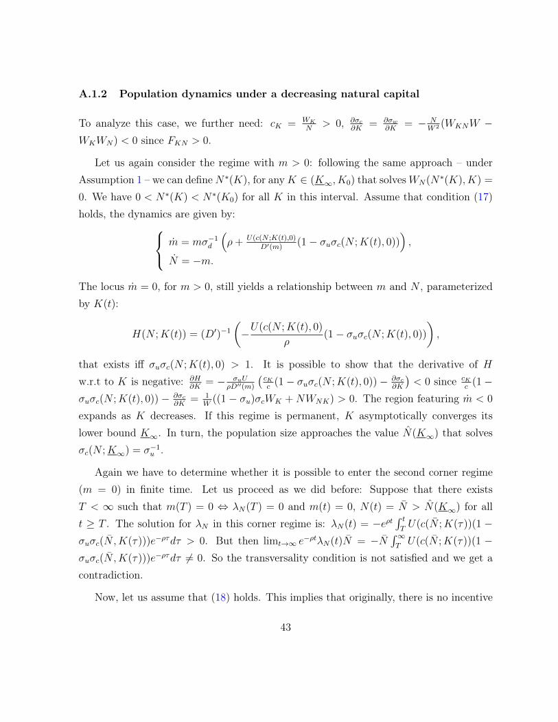
A.1.2 Population dynamics under a decreasing natural capital
To analyze this case, we further need: cK = WK
N> 0, ∂σc
∂K= ∂σw
∂K= − N
W 2 (WKNW −WKWN) < 0 since FKN > 0.
Let us again consider the regime with m > 0: following the same approach – underAssumption 1 – we can defineN∗(K), for anyK ∈ (K∞, K0) that solvesWN(N∗(K), K) =
0. We have 0 < N∗(K) < N∗(K0) for all K in this interval. Assume that condition (17)holds, the dynamics are given by: m = mσ−1
d
(ρ+ U(c(N ;K(t),0)
D′(m)(1− σuσc(N ;K(t), 0))
),
N = −m.
The locus m = 0, for m > 0, still yields a relationship between m and N , parameterizedby K(t):
H(N ;K(t)) = (D′)−1
(−U(c(N ;K(t), 0)
ρ(1− σuσc(N ;K(t), 0))
),
that exists iff σuσc(N ;K(t), 0) > 1. It is possible to show that the derivative of Hw.r.t to K is negative: ∂H
∂K= − σuU
ρD′′(m)
(cKc
(1− σuσc(N ;K(t), 0))− ∂σc∂K
)< 0 since cK
c(1−
σuσc(N ;K(t), 0)) − ∂σc∂K
= 1W
((1 − σu)σcWK + NWNK) > 0. The region featuring m < 0
expands as K decreases. If this regime is permanent, K asymptotically converges itslower bound K∞. In turn, the population size approaches the value N(K∞) that solvesσc(N ;K∞) = σ−1
u .
Again we have to determine whether it is possible to enter the second corner regime(m = 0) in finite time. Let us proceed as we did before: Suppose that there existsT < ∞ such that m(T ) = 0 ⇔ λN(T ) = 0 and m(t) = 0, N(t) = N > N(K∞) for allt ≥ T . The solution for λN in this corner regime is: λN(t) = −eρt
∫ tTU(c(N ;K(τ))(1 −
σuσc(N ,K(τ)))e−ρτdτ > 0. But then limt→∞ e−ρtλN(t)N = −N
∫∞TU(c(N ;K(τ))(1 −
σuσc(N ,K(τ)))e−ρτdτ 6= 0. So the transversality condition is not satisfied and we get acontradiction.
Now, let us assume that (18) holds. This implies that originally, there is no incentive
43

to undertake migration: m = 0 and N = N0. The evolution of λN is given by:
˙λN = ρλN − U(c(N0;K(t), 0)(1− σuσc(N0;K(t), 0))
The locus ˙λN = 0 gives a relationship:
H(N0;K) =U(c)(1− σuσc)
ρ
withHN0 = 1ρ
(cNU
′(c)(1− σuσc)− σuU(c)∂σc∂N
)= U(c)σu
ρW(WN(1− σc(σu − 1)) +N0WNN) <
0 and ˙λN > 0 for λN > H(N0;K). Under (18), this locus satisfies H(N0;K0) > 0. Now,with K decreasing, noticing that ∂σc
∂K< 0, we have σc ≤ σ−1
u ⇔F (K,N0)
N0(σ−1
u − 1 + σf ) ≥R′(M0) − (σ−1
u − 1)R(M0)N0
, with σf = NFNF
the share of labor in production. Let us workwith technologies exhibiting a constant σf ∈ (0, 1). Then, either M0 is so large that theRHS is negative and the inequality is always satisfied: the regime with m = 0 is perma-nent and has the same features as the ones studied in Appendix A.1.1. Or, M0 is lowenough – and the initial emigration ratio satisfies: M0
N0< σr(M0)
σ−1u −1
with σr(M) = MR′(M)R(M)
– for the RHS to be positive. In this case, there exists a unique K(N0) that solves theequation above and σc R σ−1
u ⇔ K Q K(N0). In turn and provided that K(N0) > K∞,this implies that the economy will experience a switch in finite time to the regime withm > 0. For K given, in a regime with m = 0, the shadow value of N should be constantand equal to H(N0;K). Now, given the continuous decrease in K, this shadow value willdecrease too still while being given by λN(t) = H(N0;K(t)).28 Let T be the date at whichλN is equal to 0: λN(T ) = 0, or equivalently K(T ) = K(N0). From T onwards, we expectthat λN(t) < 0 first, experiences a phase where it decreases and then becomes increasingand behaves according to the interior solution analyzed above. This would in turn resultsin a non-monotone trajectory for m, m being increasing first before it starts to decreaseto asymptotically approach 0.
28This confirms that the system cannot start in the regime where m > 0 (which features λN < 0 and˙λN > 0) in this case.
44

A.1.3 Dynamics of natural capital and its shadow value
Take first N as given. In the regime with s = 0, the dynamics are:{λK = (ρ+ δ)λK − FK(K,N)U ′(c(K,N, 0))
K = δ(K∞ −K)(19)
The steady state of this regime is located at the (unique) intersection between thevertical line K = K∞ and the locus λK = 0, which now defines a relation betweenK and λK : λK = FK(K,N)U ′(c)
ρ+δ≡ ζ(K;N), with ζK(K;N) = FKKU
′(c)+FKcKU′′(c)
ρ+δ< 0,
ζN(K;N) > 0, and λK ≥ 0 ⇔ λK ≥ ζ(K;N). In addition, it is quite easy to check thatthis steady state is saddle point stable. This means that convergence can occur only alongthe part of the stable branch originating in the domain where λK > 0 and K < 0. Thismakes sense: as natural capital depreciates, its social value increases during the transitionto the StS.
The next question is: can a transition from s = 0 to s > 0 occur in finite time?To provide an answer, we have to define the critical locus that divides the (K,λK) intotwo domains, one with s = 0, the other with s = 0. To do so, simply replace s = 0 inthe second FOC of system (16), and suppose that it holds with an equality. This givesanother relation between K and λK : λK = −G′(0)U ′(c)
δε′(0)K≡ ξ(K;N), with ξK(K;N) =
G′(0)U ′(c)δε′(0)K2 (1 − KcK
ccU ′′(c)U ′(c)
) < 0 and ξN(K;N) = −G′(0)cNU′′(c)
δε′(0)K> 0. Moreover, we get that
s = 0 when λK < ξ(K;N).
Then we obtain ζ(K;N) ≤ ξ(K;N) ⇔ KFK ≤ −G′(0)(ρ+δ)δε′(0)
. Given that the LHSof this inequality is equal to (1 − σf )F (K,N), so increasing in K, this is equivalent toK ≤ K(N) with K(N) = F−1
(− G′(0)(ρ+δ)
(1−σf )δε′(0);N). In addition, as it also decreasing in N ,
we can conclude that: K ′(N) < 0.
Suppose that K∞ < K(N0) < K0, then the economy with no adaptation must beoriginally located in the region with λK < 0 and K < 0, which is not compatible withthe existence of an optimal trajectory leading to the corner steady state. In other words,K(N0) > K0 is a necessary and sufficient condition for the existence of a corner solutionwith K∞ = K∞. This also implies that a transition from the corner regime with s = 0 to
45

the interior regime with s > 0 cannot take place ever.
With N decreasing, that is under positive migration, all the critical loci go downsince ζN(K;N), ξN(K;N) > 0 while K(N) moves up because of the different speeds ofadjustment of ζ(K;N) and ξ(K;N). This first means that the region where it is optimalnot to adapt shrinks over time. Clearly, in this situation, starting within the regime withs = 0, it may be possible that a switch to s > 0 occurs in finite time. But it proves verydifficult to provide formal conditions that guarantee such a transition.
A.2 Regime with positive adaptation
A.2.1 Dynamics of natural capital and adaptation
We first work with for N given. Consider the dynamics in the regime with s > 0,represented in the (K, s) plan: λK =
[ρ+ δε(s)
(1 + KFK(K,N)
G′(s)ε′(s)ε(s)
)]λK ≡ [ρ− δε(s)φ(K, s;N)]λK
K = δ(K∞ − ε(s)K)(20)
whereφ(K, s;N) = −ε
′(s)
ε(s)
1
G′(s)KFK − 1.
For a tractable analysis, from now on we consider a specification of the model withthe following functional forms: U(c) = σ−1
u cσu , σu ∈ (0, 1); D(m) = 11+σd
m1+σd , σd ≥ 1;Y = AKαN1−α, A > 0, α ∈ (0, 1); R(M) = rM , r > 0; G(s) = γs, γ > 1; andε(s) = e−ηs, η > 0.
This expression above then reduces to:
Φ(K;N) =η
γαAKαN1−α − 1,
with ΦK = ηγα2AKα−1N1−α > 0 for K ∈ [K∞, K0].
We want to deal with the features of the K = 0 and λK = 0 loci, (from which we caninfer those of s = 0 locus) given that the latter is parameterized by N . This leads to the
46

definition of two relations between s and K: λK = 0⇔ s = ε−1(ρδΦ(K;N)−1
)≡ ε(K;N),
K = 0⇔ s = ε−1(K∞K
)≡ ϕ(K).
(21)
Define K(N) such that Φ(K(N);N) = 0; K(N) =(
γηαA
Nα−1) 1α , with K ′(N) < 0. We
have K(N) > K(N0) for all N < N0. For the first relation to exist, we must focuson the interval [K(N), K0], which is non-empty only if the following condition holds:K(N0) < K0. Moreover, by definition ε(s) ∈ [0, 1] for s ≥ 0, and ε(0) = 1. This imposesa stronger restriction on the domain of definition of K: for a solution with s > 0 to be
well-defined, K should belong to [K(N), K0], with K(N) =(
γ(ρ+δ)δη(1−σF )A
Nα−1) 1α> K(N)
for the functional forms used.29 This interval is non-empty only if K(N0) < K0, as K(.)
is decreasing in N . So we impose
K(N0) < K0. (22)
Remind that K is necessarily non-increasing in our problem,30 so we must restrictthe analysis to pairs (K, s) such that K ≤ 0 ⇔ s ≤ ϕ(K). The K = 0 satisfies:ϕ′(K) = 1
ε′(.)× −K∞
K> 0. For our specification we actually get ϕ(K) = 1
ηln( K
K∞);
thus ϕ(K∞) = 1η, ϕ′(K) = 1
ηK> 0, and ϕ′′(K) = − 1
ηK2 < 0. As to the other locus,ε′(K;N) = 1
ε′(.)× −ΦK(K;N)
Φ(K;N)2> 0. Again, referring to the functional forms we use, we
obtain ε(K;N) = 1η
ln( δΦ(K;N)ρ
), εK(K;N) = ΦKΦ> 0 and εKK(K;N) = 1
ηΦKKΦ−(φK)2
Φ2 < 0.Both loci are increasing in concave inK. Given that from the second FOC in (16), λK ≥ 0,we further have λK ≥ 0 ⇔ s ≥ ε(K;N). We can finally observe that as N increases, sodoes ε(K;N) because εN(K;N) = ΦN
ηΦ> 0.
Assume for now that ϕ(K) and ε(K;N) have a unique intersection. By construction,this steady state belongs to the s = 0 locus. By differentiating the second FOC in (16),that defines the optimal s as s = s(λK , K;N), we get(
ε′′(s)
ε′(s)− cU ′′(c)
U ′(c)
csc
)ds = −
(1− cU ′′(c)
U ′(c)
KcKc
)dK
K− dλK
λK,
29Indeed, K(N) solves Φ(K(N);N) = ρδ ⇔ ε(K(N);N) = 0 and it must hold that Φ(K(N);N) ≥ ρ
δ .30A restriction that we didn’t incorporate in the optimization program for simplicity, but that has to
be verified ex-post.
47

noticing that ε′′(s)ε′(s)
= −η, − cU ′′(c)U ′(c)
= 1 − σu and using the specifications, this expressionssimplifies to:
ds =
(η +
γ(1− σu)Nc
)−1 [(1 +
KFK(1− σu)Nc
)dK
K+dλKλK
], (23)
which means that sK > 0, sλK > 0 and sN < 0. From that, we directly obtain theexpression of s, whose sign is undetermined when λK > 0, given that K < 0 (exceptat the steady state). We come back to this later on. In the meantime, the steady stateanalysis is conducted.
We still work for N given and look at the conditions for the existence of a steadystate (K∞(N), s∞(N)). From (21), a steady state solves: ϕ(K) = ε(K;N). This boilsdown to finding the solution to: ρ
δKK∞
= Φ(K;N). Under (22), given that ΦK > 0 and
Φ(K(N), N) = ρδ< ρ
δK(N)K∞⇔ K(N) > K∞, if we impose:{
K(N0) < K∞,
Φ(K0;N0) < ρδK0
K∞,
(24)
then we know that there exists a unique K∞(N) ∈ (K(N), K0) solving the equationabove. Actually, K∞(N) must be larger than K∞: K∞(N) ∈ (K∞, K0). In addition,K∞(N)′(N) > 0 as ΦN(K;N) > 0. We finally obtain s∞(N) by replacing K with K∞(N)
in for instance ϕ(K), with s′∞(N) = ϕ′(K)K ′∞(N) > 0.
Let us now assess the local stability conditions, for N given. Equation (23) yieldss = 0 in terms of λK and K, replacing them with the corresponding law of motion, weget:
s = δ
(η +
γ(1− σu)Nc
)−1(Λ(K;N) +
(1− σu)(1− σf )F (K,N)
Nc
(K∞K− ε(s)
))(25)
with Λ(K, s) = ρδ
+K∞K
+(1−σf )ε′(s)F (K,N)
γ. Combining this equation with the expression
for K, and linearizing around the steady state, we obtain the Jacobian matrix, J :
J =
− δ(1−σf )ε′(s)F (K,N)
γ
δ(η+γ(1−σu)Nc )
−1
K
((1−σf )2ε′(s)F (K,N)
γ− (1 +
(1−σu)(1−σf )F (K,N)
Nc)K∞K
)−δε′(s)K −δε(s)
48

Direct calculations yield:
det J = δ2ε′(s∞(N))ε(s∞(N)) (σf (1 + Φ(K∞(N);N))− 1) < 0⇔ Φ(K∞(N);N)) >1− σfσf
,
and under this condition, the steady state (K∞(N), s∞(N)) is a saddle point.
The convergence to the steady state takes place along the stable branch, which meansthat both s andK follow a monotone path. Note that the second term between parenthesisin (25) is always negative. Now assume that s > 0 for all t. We have Λ(K∞(N), s∞(N)) =
0, and s < s∞(N) and K > K∞(N) for any pair (K, s) in the neighborhood of the steadystate. Given that ΛK < 0 and λs > 0, Λ(K, s) < Λ(K∞(N), s∞(N)) = 0. This inturn implies that s < 0 at the instant when the pair (K, s) is achieved, which yields acontradiction. So we can claim that s is monotone decreasing over time.
A.2.2 Migration and population dynamics
From here, we do not really provide a formal proof but rather a discussion on the possibleoutcomes.
In the last step of the resolution, we move back to the analysis in the (N, λN), or(N,m), plan. Following the same lines as in the Appendices A.1.1 and A.1.2, we alreadyknow that the properties of σc are decisive to characterize the solution. Before we proceed,it is worth noticing that the general definition of σc has changed:
σc(N ;K, s) = − 1
Nc(G(s)−W (1 + σw(N,K)))⇔ σc(N ;K, s) = 1 +
Wσw(N,K)
W −G,
with
∂σc∂N
= − cNc
(σc − 1 + WNN
CN
)> 0,
∂σc∂K
= − 1(Nc)2
(GWKσw + N(W−G)
W(WNKW −WKWN)
)= − N
(Nc)2((W −G)WNK −WKWN) < 0,
∂σc∂s
= G′(s)Wσw(Nc)2
= −γNWN
(Nc)2> 0.
(26)
We observe that σc(N ;K, s) > σc(N ;K, 0) for all s > 0. Assume that condition(17) holds. This implies that σc(N0;K0, s0) > σ−1
u : there will be incentive to migrate
49

initially. For s > 0 and K given, we further know that ∃! N∗(K) ∈ (0, N0) such thatσc(N
∗(K);K) = 1 < σ−1u . Taking the pair (K, s) as given, it must exists a unique
solution to σc(N ;K, s) = σ−1u . Denote this solution as N(K, s). But this does not
solve the existence issue: we want to be sure that there exists N ∈ (0, N0) that solvesσc(N ;K∞(N), s∞(N)) = σ−1
u . This is not obvious as if we know that σc may be varyingfor at least some period of time in the interval (1, σ−1
u ) and is continuous w.r.t. t, it isdifficult to understand how it will change over time because it depends on N , K and s.To be completed.
Next we can use the relation s = ϕ(K) ≡ s(K) to define the steady state populationsize as a function of K only: N(K) = N(K, s(K)). Then, we compute
N ′(K) = −(∂σc∂K
+ ∂σc∂ss′(K)
)∂σc∂N
Direct manipulations give:
∂σc∂K
+∂σc∂s
s′(K) < − γΦ(K;N)
ηK(W −G)2≤ 0 for K ≥ K(N).
Thus, the numerator above is non-negative, which means that a necessary and sufficientcondition for N ′(K) > 0 is ∂σc
∂N> 0, which is indeed the case. There is a clear parallel to
draw between the current analysis and the one conducted in the Appendix A.1.2. Indeed,the solution we get in this benchmark case can be rewritten (with slight abuse of notation)as N(K∞, 0). Moreover, the solution is clearly continuous in (K, s). As N is increasingin s but decreasing in K we then conclude that N(K, s(K)) > N(K∞, 0) for K > K∞
and s(K) > 0.
Now consider that condition (18) holds. Compared to the benchmark, this is onlynecessary for a regime m = 0 to take place initially. Assume that this is indeed the case,which requires s(0) be low enough: σc(N ;K, s(0)) < σ−1
u . Then the question is: would atransition in finite time be possible in this situation? In other words, we want to check towhich extent the analysis conducted in the Appendix A.1.2 can still apply to the generalcase. With N constant and equal to N0 initially (as m = 0), we have to study the impactsof the dynamic adjustments in (K, s) on migration incentives. Basically, this boils down
50

to tracking the evolution of σc across time, given that: σc = ∂σc∂KK + ∂σc
∂ss. Rearranging
(that is, using the expression of s, K and of the partial derivatives), we get
σc =− NK
(Nc)2
(η +
γ(1− σu)
Nc
)−1
×
[((W −G)
(η +
γ(1− σu)
Nc
)− γWN
KΦ(K,N)
)K
K+γWN
K
λKλK
]
This expression is positive if λK > 0 in this regime. The steady state, analyzed in the(K,λK), is a saddle point, which implies that λK must be monotone. In addition, it isclear that K > 0 in the neighborhood of the steady state, with
K =− δε(s)K
(−ηs+
K
K
)
= δε(s)K
(η +
γ(1− σu)
Nc
)−1(ηλKλK
+γ(1− σu)Φ(K,N)
Nc
K
K
),
a necessary condition for this to be true is limt→∞ λK > 0. Thus λK > 0 for all t < ∞.In sum, σc is increasing over time in this regime. The last question is, will it reach thethreshold σ−1
u , that triggers migration, in finite time? The answer depends on the featuresof the steady state (K∞(N0), s∞(N0)). Actually, we can conclude that a transition to theregime with m > 0 will occur in finite time if and only if
σc(N0;K∞(N0), s∞(N0)) > σ−1u . (27)
A.3 Further elements
A.3.1 Natural capital dynamics, with and without adaptation
Denote respectively by Ks and K0 the stock of capital corresponding to a situation withpermanent adaptation and no adaptation at all. We want to show that Ks(t) > K0(t)
for all t. Let us work by contradiction.
51

We know that Ks∞ = K∞(N) > Ks
∞ = K∞ and Ks(0) = K0(0) = K0. MoreoverKs(0) = δ(K∞ − ε(s(0))K0) > Ks(0) = δ(K∞ − K0) because ε(s(0)) < 1 for s(0) > 0.So in the neighborhood of t = 0, Ks > K0. If there exist instants at which Ks and K0
take the same value, the number of such instants must be even. Assume that there existstwo instants (t1, t2), with t1 < t2 such that Ks(t1) = K0(t1) and Ks(t2) = K0(t2). Wenecessarily have Ks(t1) < K0(t1). This is equivalent to ε(s(t1)) > 1, which is impossible.This yields the contradiction and we can claim that Ks(t) > K0(t) for all t.
A.3.2 Critical threshold K(N0) for the specified model
For our specifications, we get:
K(N0) =
[r (N0 − (σ−1
u − 1)M0)Nα−10
A(σ−1u − α)
] 1α
,
it is linear in N0 forM0 = 0, and well defined forM0 > 0 provided that M0 is low enough.
A.4 Calibration
In this section we provide details on the calibration of the theoretical analysis
developed in section 5.
A.4.1 Model Specification
The functional forms used at the different stages of the analysis are the following:
• Power functions with D(m) = 11+σd
m1+σd , σd ≥ 1, and U(c) = 1σucσu , σu ∈ (0, 1).
• Cobb-Douglas technology:Y = AKαN1−α, and linear remittances: R(M) = rM .Then σF = 1− α, σR = N
N0−N , and σ′R = N0
N0−N = (1+σR)N0−N > 0.
• Linear cost of infrastructure expenditure G(s) = γs, with γ > 1 the cost of publicfunds, and ε(s) = e−ηs.
52

A.4.2 Parameters description
A.4.3 Comparative statics
In this section we show that the model is robust to changes in the parameters, and thatthe conclusion for the analysis of the initial conditions are the same for reasonable changesin the parameters values.
Figure 13: Analysis of the effects of the parameter A on K
10-1
100
101
Population
102
103
104
Natu
ral C
apital
Other SIDS
COM
CPV
FJI
GNB
MDV
MUS
STP
SYC
K hat
A=0.99
A=1
A=1.02
10-1
100
101
Population
102
103
104
Natu
ral C
apital
Caribbean SIDS
ABW
ATG
BHS
BLZ
BRBCUW
DMA
DOM
GRD
HTI
JAM
LCASUR
TTO
VCT
K hat
A=0.99
A=1
A=1.02
Figure 14: Analysis of the effects of the parameter σu
10-1
100
101
Population
102
103
104
Natu
ral C
apital
Other SIDS
COM
CPV
FJI
GNB
MDV
MUS
STP
SYC
K tilde
σu=0.9
σu=0.95
σu=0.99
10-1
100
101
Population
102
103
104
Natu
ral C
apital
Caribbean SIDS
ABW
ATG
BHS
BLZ
BRBCUW
DMA
DOM
GRD
HTI
JAM
LCASUR
TTO
VCT
K tilde
σu=0.9
σu=0.95
σu=0.99
53

Table 4: Country level of the TFP
Cap. (AFF and Tourism) Cap. (All Stocks)
Countries (1) (2) (1) (2)
Comoros 1 1 1.01 1.01Cabo Verde 1.01 1.02 1.01 1.01Fiji 1.01 1.02 0.98 0.99Guinea-Bissau 1.00 1.00 1.00 1.01Maldives 1.02 1.04 1.00 1.02Mauritius 1.00 1.01 0.98 0.98Sao Tome and Principe 1.02 1.02 1.00 1.00Seychelles 1.03 1.03 1.02 1.03Aruba 0.99 0.99 0.97 0.97Antigua and Barbuda 1.10 1.02 1.04 1.01Bahamas, The 0.98 0.99 0.92 0.92Belize 1.00 1.01 0.98 0.99Barbados 0.96 0.96 0.94 0.93Curacao 0.99 0.98Dominica 0.83 0.97 0.8 0.96Dominican Republic 1.03 1.03 1.01 1.01Grenada 0.98 0.99 0.98 1.00Haitit 0.97 0.97 0.96 0.97Jamaica 1.02 1.02 0.97 0.98Saint-Lucia 1.01 1.01 0.98 0.99Suriname 1.03 1.03 1.00 1.00Trinidad and Tobago 1.08 1.08 0.99 0.99Saint-Vinc. and the Gren. 0.99 1.00 0.95 0.96
Average 1.00 1.01 0.98 0.99Maximum 1.10 1.08 1.04 1.03Minimum 0.83 0.96 0.8 0.92
Legend: (1): Labor is given by Employment (PWT), (2) Labor is given by the Popula-tion (PWT) 54

Table 5: Correlation coefficient between computed output and observed output (PWT)
Cap. (All stocks) Cap. (AFF and Tourism)
Countries group (1) (2) (1) (2)
SIDS 0.93 0.92 0.93 0.89Developing Countries 0.6 0.8 0.61 0.78Developed Countries 0.85 0.89 0.86 0.89
Legend: (1): Labor is defined as the Employment from the PWT, (2): Labor is definedas the Population from the PWT.
Figure 15: Analysis of the effects of the parameter γ
10-1
100
101
Population
102
103
104
Natu
ral C
apital
Other SIDS
COM
CPV
FJI
GNB
MDV
MUS
STP
SYC
K hat
γ=1
γ=1.2
γ=1.5
10-1
100
101
Population
102
103
104
Natu
ral C
apital
Caribbean SIDS
ABW
ATG
BHS
BLZ
BRBCUW
DMA
DOM
GRD
HTI
JAM
LCASUR
TTO
VCT
K hat
γ=1
γ=1.2
γ=1.5
55

Figure 16: Analysis of the effects of the parameter ρ
10-1
100
101
Population
102
103
104
Natu
ral C
apital
Other SIDS
COM
CPV
FJI
GNB
MDV
MUS
STP
SYC
K hat
ρ=0.04
ρ=0.1
ρ=0.2
10-1
100
101
Population
102
103
104
Natu
ral C
apital
Caribbean SIDS
ABW
ATG
BHS
BLZ
BRBCUW
DMA
DOM
GRD
HTI
JAM
LCASUR
TTO
VCT
K hat
ρ=0.04
ρ=0.1
ρ=0.2
Figure 17: Analysis of the effects of the parameter A on K
10-1
100
101
Population
102
103
104
Natu
ral C
apital
Other SIDS
COM
CPV
FJI
GNB
MDV
MUS
STP
SYC
K hat
A=0.99
A=1
A=1.02
10-1
100
101
Population
102
103
104
Natu
ral C
apital
Caribbean SIDS
ABW
ATG
BHS
BLZ
BRBCUW
DMA
DOM
GRD
HTI
JAM
LCASUR
TTO
VCT
K hat
A=0.99
A=1
A=1.02
56