Vortex Mode Bifurcation and Lift Force of a Plunging ...people.bath.ac.uk/en3djc/AIAA FINAL PAPER - David Cleaver (10_01).pdf · vortex strength, nor at larger angles ... The LEV

1

American Institute of Aeronautics and Astronautics

Vortex Mode Bifurcation and Lift Force of a Plunging

Airfoil at Low Reynolds Numbers

D.J. Cleaver*, Z. Wang

†, and I. Gursul

‡

University of Bath, Bath, BA2 7AY, United Kingdom

Force and supporting particle image velocimetry measurements were performed on a

plunging NACA 0012 airfoil at a Reynolds number of 10,000, at pre-stall, stall, and post-stall

angles of attack. The lift coefficient for pre-stall and stall angles of attack at larger

amplitudes showed abrupt bifurcations with the branch determined by initial conditions.

With the frequency gradually increasing, very high positive lift coefficients were observed,

this was termed mode A. At the same frequency with the airfoil impulsively started, negative

lift coefficients were observed, this was termed mode B. The mode A flow field is associated

with trailing-edge vortex pairing near the bottom of the plunging motion causing an

upwards deflected jet, and a resultant strong upper surface leading-edge vortex. The mode B

flow field is associated with trailing-edge vortex pairing near the top of the plunging motion

causing a downwards deflected jet, and a resultant weak upper surface leading-edge vortex.

The bifurcation was not observed for small amplitudes due to insufficient trailing-edge

vortex strength, nor at larger angles of attack due to greater asymmetry in the strength of

the trailing-edge vortices, which creates a natural preference for a downward deflected

mode B wake.

Nomenclature

a = amplitude of plunging motion

Cl = time-averaged lift coefficient

c = chord length

d = trailing-edge vortex separation distance

f = frequency

Re = Reynolds number, ρU∞c/ µ

Src = Strouhal number based on chord, fc/U∞

SrA = Strouhal number based on amplitude, 2fa/U∞

UP = peak plunge velocity, 2πfa t = time, 0 is top of motion

T = plunge period

U∞ = free stream velocity

V = velocity magnitude

α = angle of attack

αeff,min = minimum effective angle of attack

αeff,max = maximum effective angle of attack

αvortex = trailing-edge vortex trajectory angle

Γ = vortex circulation

ΓT- = clockwise trailing-edge vortex circulation

ΓT+ = counter-clockwise trailing-edge vortex circulation

µ = viscosity

ρ = density

* Postgraduate Student, Department of Mechanical Engineering, Student Member AIAA. † RCUK Academic Fellow, Department of Mechanical Engineering, Member AIAA. ‡ Professor, Department of Mechanical Engineering, Associate Fellow AIAA.

2


I. Introduction

atural flight presents an excellent example of the type of performance desirable for Micro Air Vehicles1, i.e.,

the ability to cruise efficiently, maneuver, and hover at low Reynolds numbers in restricted space. This

performance is inexplicable through steady-state aerodynamic theory; instead birds and insects rely on unsteady

aerodynamic phenomenon2. Therefore for MAVs to achieve similar performance man must likewise look to

unsteady aerodynamics for the solution3.

Within nature the primary unsteady aerodynamic phenomenon responsible for lift augmentation is the Leading Edge

Vortex (LEV)4-7. The LEV is a region of highly three-dimensional recirculation produced during the wing’s

downstroke. It acts to create a region of low pressure over the upper surface of the wing, although it can also be

considered as augmenting the circulation around the wing, and thus increases lift. To produce the LEV natural flyers

rely on a complex combination of flexing, twisting, bending, rotating or feathering during the flapping cycle2. Due

to actuator, sensor, and control limitations creating similar wing kinematics on a practical aircraft will be very

challenging.

A potential intermediate solution is instead of using the large-amplitude low-frequency flapping motion suited to

muscular actuators, to use small-amplitude high-frequency pure plunging motion as is suited to electrical actuators.

This design would combine both the controllability of fixed-wing designs with the enhanced performance of

flapping-wing unsteady aerodynamics allowing for improved cruise and gust performance. This idea was originally

derived from delta wing aerodynamics research8 where small-amplitude roll oscillations, and latterly passively

induced vibrations resultant from wing flexibility9, were shown to improve performance. When applied to a NACA

0012 airfoil at a fixed post-stall angle of attack this type of motion has been shown to produce significant lift

enhancement10,11

(~ three times the steady-state lift coefficient) in addition to being thrust producing12. The lift

enhancement was attributed to greater circulation of the upper surface LEV relative to the lower surface LEV. In

essence the asymmetry created by the fixed angle of attack creates asymmetry in the vortex strengths and thus lift.

Correspondingly, if one was to plunge an airfoil at zero degrees angle of attack one would presume that the flow

field over upper and lower surface would be symmetrical and therefore produce zero time-averaged lift. However

previous results13-17

have demonstrated that this may not be true at higher plunge velocities because pairing of the

trailing-edge vortices causes the wake to become deflected upwards or downwards creating an asymmetric flow

field, and therefore presumably non-zero time-averaged lift. The direction of the jet is determined by the initial

conditions13 (moving upwards or downwards), and this direction may switch periodically

15 (with a period on the

order of 100/f). These previous studies13-17

were limited to symmetric variations in angle of attack.

For an asymmetric variation in angle of attack (nonzero mean), this paper presents experiments that demonstrate a

similar deflected jet for small-amplitude (a/c < 0.20) plunging motion at pre-stall and stall angles of attack (α = 5°

and 10°). For the first time lift force measurements are presented along with accompanying PIV results, and a new

set of criteria are presented for the onset of jet deflection.

II. Experimental Apparatus and Procedures

Force and PIV measurements were conducted on a plunging NACA 0012 airfoil mounted vertically in a closed-loop

water tunnel. For a review of parameters studied, see Table 1; uncertainties are calculated based on the methods of

Moffat18 taking into account both bias and precision errors.

Table 1 Experimental Parameters

Parameter Range Considered Uncertainty

Re 10,000 – 40,000 +/- 200

α 5° to 15° +/- 0.5°

a/c 0.025 to 0.200 +/- 0.003

Src 0 to 3 +/- 2.3%

A. Experimental Setup The experiments were conducted in a free-surface closed-loop water tunnel (Eidetics Model 1520) at the University

of Bath. The water tunnel is capable of flow speeds in the range 0 to 0.5 m/s and has a working section of

dimensions 381 mm x 508 mm x 1530 mm. The turbulence intensity has previously19 been measured by LDV to be

less than 0.5%.

N

3


A NACA 0012 airfoil of dimensions 0.1 m chord x 0.3 m span was mounted vertically in a 'shaker' mechanism, see

Fig. 1. The airfoil was constructed by rapid prototyping from SLS Duraform Prototype PA. It was placed between an

upper and lower splitter plate, clearances were maintained at 2 mm. The oscillations were supplied via a Motavario

0.37 kW three-phase motor, 5:1 wormgear and IMO Jaguar Controller. The position of the root of the airfoil was

measured through a rotary encoder attached to the spindle of the worm gear shaft. The rotary encoder was also used

to trigger the PIV system.

B. Force Measurements The forces applied in both the x and y directions were measured via a two-component aluminium binocular strain

gauge force balance20. The measured forces included both time-dependent aerodynamic forces as well as inertia

forces, however the inertia forces do not contribute to the time-averaged force. Two force balances were used, a

more rigid (less sensitive) one for the dynamic cases, and a more flexible (more sensitive) one for the stationary

cases. The signal from the strain gauges was amplified by a Wheatstone bridge circuit and sampled at either 2 kHz

for 20,000 samples (stationary cases), or 360 per cycle for a minimum of 50 cycles (dynamic cases). The forces

were then calculated from the average voltage through linear calibration curves. To minimize uncertainty the

calibration curves consisted of twenty three points, and were performed daily before and after testing. Each data set

was repeated at least once and then averaged. The mean lift coefficient uncertainty for the stationary case is ± 0.03.

C. PIV Measurements A TSI 2D-PIV system was used to measure the velocity field in the vicinity of the airfoil. For measurements over

the upper surface of the airfoil, the laser was positioned behind as shown in Fig. 1. The shadow created by the airfoil

therefore obscured the lower surface. For measurements over the lower surface the laser was positioned near the side

wall of the tunnel. In both cases, the camera was located under the tunnel as shown in Fig. 1. The PIV images were

analyzed using the software Insight 3G. A recursive FFT correlator was selected to generate a vector field of

199x148 vectors giving approximately a 1.2 mm spatial resolution for the upper surface, and 0.9 mm for the lower

surface. The time-averaged data is derived from 500 pairs of images, the phase-averaged from 100 pairs for the

upper surface and between 100 and 250 pairs (as required) for the lower surface. The upper and lower surface data

were later merged through interpolation of the lower surface data onto the upper surface grid in MATLAB.

To calculate the circulation from the phase-averaged data, first the vortex is located using a vortex identification

algorithm21,22

with the search centered on the point of maximum / minimum vorticity as appropriate. The radius of

the vortex is then determined by continually expanding from the centre, one spatial resolution unit at a time, until the

increase in circulation is negative or small (<1%). The circulation calculation itself is done using both line integral

and vorticity surface methods17. The agreement between the two was generally very good. All circulation results

presented herein are derived from the average of the two methods.

III. Results and Discussion

A. Stationary Airfoil As a comparative case the force measurements for the stationary two-dimensional NACA 0012 airofil are presented

in Fig. 2a. Also shown are two comparative sets from the literature. The data of Sunada et al.23 is for a lower

Reynolds number, finite wing. The aspect ratio in this case was AR = 6.75, and it can therefore be considered as a

good approximation to the two-dimensional case23. Likewise the data of Schluter

24 is for a finite wing, however the

aspect ratio is large (AR = 5), and the tip clearance small (1/6 c). It can therefore also be considered as a good

approximation to the two-dimensional case.

Comparing the current data set for Re = 3x104 with that from Schluter at Re = 3.1x10

4 one can see reasonable

agreement between the two sets. At small angles of attack both curves are nonlinear with the current data

consistently lower, perhaps due to freestream turbulence or surface roughness affecting the behaviour of the laminar

separation bubble. The curve of Schluter stalls at α = 9° whereas for the current data the stall angle is α = 10°. In

both cases stall is abrupt suggesting leading edge stall. Comparing the data set for Re = 1x104 with that of Sunada et

al. for Re = 0.4x104 there are very large differences. The lower Reynolds curve of Sunada et al. is consistently

lower. This is part of a general trend of decreasing lift curve slope with decreasing Reynolds number for Re < 2x104.

Furthermore, the type of stall is very different for Re < 2x104. The peak is much more rounded and the drop much

less abrupt, suggesting trailing-edge stall. This is in agreement with the flow visualization results of Huang & Lin25

4


for a NACA 0012 airfoil. They showed that for Re < 2x104 trailing-edge stall commences at angles of attack in the

region of 1°, becoming fully stalled once the angle of attack exceeds ~10°. When the Reynolds number is increased,

at a critical value the separated laminar flow will trip into turbulence and therefore reattach forming the laminar

separation bubble typical of leading-edge stall. Hence the curves for Re ≥ 2x104 are typical of leading-edge stall,

and those for Re < 2x104 are typical of laminar trailing-edge stall (as confirmed through the time-averaged flow for

α = 5 ° in Fig. 2b), with a variable gradient due to the Reynolds dependence of the laminar separation point.

Regardless of the type of stall, the location of stall is relatively consistent: α = 10°±1. The angles of attack under

consideration in this paper can therefore be classified as: α = 5° is pre-stall, α = 10° is stall, and α = 15° is fully

stalled. Corresponding time-averaged velocity fields supporting this description are shown in Fig. 2b.

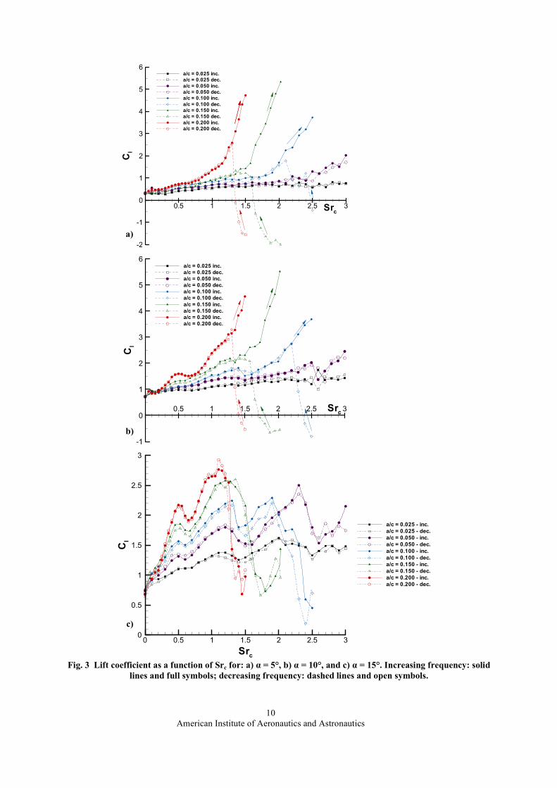
B. Force Bifurcations of Oscillating Airfoil Shown in Fig. 3 are the time-averaged lift coefficients for five different plunge amplitudes for each of the three

angles of attack considered. For each amplitude there are two separate curves, increasing (inc.) and decreasing

(dec.). Increasing represents the lift coefficients obtained when the airfoil starts at Src = 0 and the Strouhal number is

gradually increased accumulating data along the way. Decreasing represents the lift coefficients obtained when the

airfoil is impulsively started at the maximum Strouhal number and then the Strouhal number gradually decreased

accumulating data along the way.

For the majority of cases the curves for increasing and decreasing frequency are identical to within the bounds of

experimental uncertainty and can therefore be considered as the same. They all show an amplitude-dependent

increase, and share a common peak at Src = 0.45 as previously described10, with further peaks in certain cases.

However for α = 5° and α = 10° (Fig 3a and 3b) when a/c ≥ 0.100 there are very large and significant differences

between the increasing and decreasing curves. Initially both curves are identical, however at a critical Strouhal

number the two curves diverge significantly. The gradient of the increasing frequency curve becomes steeper

resulting in a maximum recorded lift coefficient of Cl = 5.5; simultaneously the gradient of the decreasing frequency

curve becomes negative resulting in a minimum recorded lift coefficient of Cl = -2.0. The values of lift coefficient

(in the case of decreasing frequency) were found to be insensitive to changes in the airfoil starting position (top,

middle or bottom). No switching between the two branches of lift coefficient was observed.

It is important to note that this bifurcation is not ubiquitous. It is only observed for α ≤ 10° (α = 12.5° and α = 20°

have also been tested but are not shown here), and a/c ≥ 0.100. Amplitude also has a very strong effect in

determining the point of bifurcation, i.e., from Fig 3a, for a/c = 0.025 and 0.050 there is no bifurcation, for a/c =

0.100 it is at Src ≈ 2, for a/c = 0.150 it is at Src ≈ 1.5, and for a/c = 0.200 it is at Src ≈ 1.3. This implies a dependence

on constant plunge velocity which shall be considered later in this paper.

Although not presented here the same bifurcations are observed in the time-averaged drag coefficient but the effect

is not as severe. Typical values for Src = 2.025 and α = 5° are Cd = -1.5 for increasing frequency, compared to Cd = -

2.5 for decreasing frequency. Even though this may seem large it is important to remember that the difference in

drag coefficient of ∆Cd ≈ 1 accompanies a difference in lift coefficient of ∆Cl ≈ 7.5, the effect on drag is therefore

comparatively small.

C. Flow Field The time-averaged flow field for a typical bifurcating case is shown in Fig. 4. Mode A refers to the flow field

associated with increasing frequency; and mode B refers to the flow field associated with decreasing frequency. This

terminology is only applicable after the point of bifurcation. Before the point of bifurcation the terminology ‘pre-

bifurcation’ shall be used.

Fig. 4 demonstrates very clearly the difference between the two modes. Mode A is associated with a time-averaged

jet that is deflected upwards and a region of high velocity magnitude over the upper surface, thus explaining the

high lift coefficient. Conversely mode B is associated with a downwards deflected jet and a region of high velocity

magnitude over the lower surface, thus explaining the negative lift coefficient. When comparing the two modes

with the pre-bifurcation flow field, it is clear that the mode A wake bears a closer resemblance (high velocity

magnitude over upper surface and jet inclined slightly upwards), implying that the mode A wake is the continuation

of the pre-bifurcation wake. This is discussed in more detail later. An interesting feature of Fig. 4 is that the mode A

upwards deflected jet is associated with high lift and the downwards deflected jet is associated with low / negative

lift.

5


To understand the underlying flow physics behind the time-averaged flow field it is necessary to look to the phase-

averaged flow field. Fig. 5 shows phase-averaged vorticity contour plots for four points in the cycle for the same

cases as in Fig. 4. The most significant difference between modes is the trailing-edge vortex behavior. In the case of

mode A the clockwise trailing-edge vortex after shedding remains near the trailing-edge, causing premature

formation of the counter-clockwise trailing-edge vortex (see phase a). Consequently the two pair near the bottom of

the motion (phases b & c) and due to their respective positions convect in an upwards direction. In the case of mode

B this process is inverted, i.e., the counter-clockwise vortex remains near the trailing-edge causing premature

formation of the clockwise trailing-edge vortex (phase c), the two pair and convect downwards (phases d & a). The

crucial parameter in determining the direction of the deflected jet is therefore the timing of the vortex-pairing

process. Once the vortex pairing starts in a particular manner it will then be ‘locked-in’ since at high plunge

velocities only two trailing-edge vortices are created per cycle, and the manner in which they pair (clockwise to

counterclockwise or vice-versa) determines which vortex is created first in the next cycle and thus the next cycle’s

pairing process. The flow field is therefore ‘locked-in’ to that mode.

At the leading-edge, the region of high velocity magnitude observed in the time-averaged data is shown to be due to

strong leading-edge vortices. The circulation of these leading-edge vortices is quantified in Fig. 6. Note that for

convenience the pre-bifurcation data is treated as an extension of the mode A although it is common to both. Even

though there is a difference in the strength of all the vortices between a mode A and B flow field, it is the circulation

of the upper surface clockwise leading-edge vortex which changes most dramatically. At Src = 2.025 the mode A

upper surface leading-edge vortex is approximately twice the circulation of the mode B. This is also evident in Fig.

5c. Furthermore the mode B flow field is associated with a stronger lower surface leading-edge vortex, explaining

both the regions of high time-averaged velocity magnitude, and low values of lift coefficient. The difference in

leading-edge vortex strength can be attributed to the deflection of the jet. When upward deflected (mode A) it will

draw fluid from the upper surface thereby enhancing the upper surface leading-edge vortex; conversely when

downwards deflected (mode B) it will draw fluid form the lower surface thereby enhancing the lower surface

leading-edge vortex.

From consideration of Fig. 6 it is suggested that the Mode A wake is a continuation of the pre-bifurcation wake.

This is also reflected in the similarity of the pre-bifurcation flow field to the mode A flow field in both Fig. 4 and

Fig. 5. Indeed this is entirely plausible as before the point of bifurcation the jet is consistently deflected upwards.

The pre-existing wake therefore acts as an initial condition creating a natural ‘preference’ for the mode A flow field.

The general trends shown in Fig.s 4, 5, and 6 are repeatable for all bifurcating amplitudes and angles of attack. Fig.

7 and Fig. 8 demonstrate the effect of angle of attack on the mode A and mode B flow field. Both figures show the

same pattern as previously described. Mode A is characterized by trailing-edge vortex pair formation near the

bottom of the motion resulting in vortex convection in an upward direction which reinforces the upper surface

leading-edge vortex. Mode B is characterized by trailing-edge vortex pair formation near the top of the motion

resulting in vortex convection in a downward direction that inhibits the upper surface leading-edge vortex.

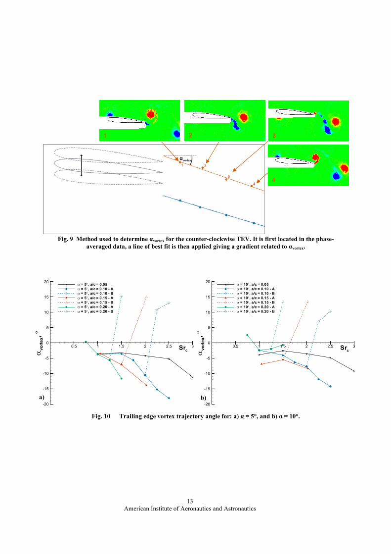
The effect of amplitude can be demonstrated through the trailing-edge vortex pair convection angle. This is derived

by tracking the trailing edge vortex position in the phase-averaged data and applying a line of best fit. The gradient

of this line then gives the angle of the convecting vortices relative to the horizontal (see Fig. 9). This is repeated for

both the clockwise and counter-clockwise trailing-edge vortices, and the average of the two is shown in Fig. 10. It

shows that across different amplitudes the pattern is similar. The pre-bifurcation wake is associated with an upwards

deflected jet and the mode A wake is a continuation of this, whereas the mode B wake is associated with a

downwards deflected jet.

D. Bifurcation Criteria An interesting feature of Fig. 3 is the amplitude dependence of the point of bifurcation suggesting the possibility that

the point of bifurcation depends upon a constant plunge velocity. Fig. 11 shows SrA (effectively plunge velocity)

versus the maximum and minimum effective angle of attack. The points of bifurcation for the different amplitudes

are shown as symbols. These points fall within a band of SrA = 0.40 ± 0.05. It can therefore be said that a minimum

plunge velocity is required for bifurcation to occur. This potentially explains why there is no bifurcation for a/c =

0.025 and a/c = 0.050 as in both cases the plunge velocity is too small, SrA < 0.30. This is however not a universal

criteria since, as shown in Fig. 11, the required SrA increases with increasing amplitude. In addition, neither plunge

6


velocity nor effective angle of attack give an adequate explanation as to why there is no bifurcation at greater angles

of attack (α > 10°).

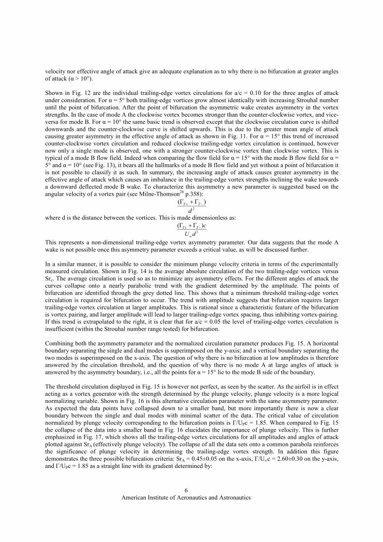
Shown in Fig. 12 are the individual trailing-edge vortex circulations for a/c = 0.10 for the three angles of attack

under consideration. For α = 5° both trailing-edge vortices grow almost identically with increasing Strouhal number

until the point of bifurcation. After the point of bifurcation the asymmetric wake creates asymmetry in the vortex

strengths. In the case of mode A the clockwise vortex becomes stronger than the counter-clockwise vortex, and vice-

versa for mode B. For α = 10° the same basic trend is observed except that the clockwise circulation curve is shifted

downwards and the counter-clockwise curve is shifted upwards. This is due to the greater mean angle of attack

causing greater asymmetry in the effective angle of attack as shown in Fig. 11. For α = 15° this trend of increased

counter-clockwise vortex circulation and reduced clockwise trailing-edge vortex circulation is continued, however

now only a single mode is observed, one with a stronger counter-clockwise vortex than clockwise vortex. This is

typical of a mode B flow field. Indeed when comparing the flow field for α = 15° with the mode B flow field for α =

5° and α = 10° (see Fig. 13), it bears all the hallmarks of a mode B flow field and yet without a point of bifurcation it

is not possible to classify it as such. In summary, the increasing angle of attack causes greater asymmetry in the

effective angle of attack which causes an imbalance in the trailing-edge vortex strengths inclining the wake towards

a downward deflected mode B wake. To characterize this asymmetry a new parameter is suggested based on the

angular velocity of a vortex pair (see Milne-Thomson26 p.358):

2

)(

d

TT −+Γ+Γ

where d is the distance between the vortices. This is made dimensionless as:

2

)(

dU

cTT

∞

−+Γ+Γ

This represents a non-dimensional trailing-edge vortex asymmetry parameter. Our data suggests that the mode A

wake is not possible once this asymmetry parameter exceeds a critical value, as will be discussed further.

In a similar manner, it is possible to consider the minimum plunge velocity criteria in terms of the experimentally

measured circulation. Shown in Fig. 14 is the average absolute circulation of the two trailing-edge vortices versus

Src. The average circulation is used so as to minimize any asymmetry effects. For the different angles of attack the

curves collapse onto a nearly parabolic trend with the gradient determined by the amplitude. The points of

bifurcation are identified through the grey dotted line. This shows that a minimum threshold trailing-edge vortex

circulation is required for bifurcation to occur. The trend with amplitude suggests that bifurcation requires larger

trailing-edge vortex circulation at larger amplitudes. This is rational since a characteristic feature of the bifurcation

is vortex pairing, and larger amplitude will lead to larger trailing-edge vortex spacing, thus inhibiting vortex-pairing.

If this trend is extrapolated to the right, it is clear that for a/c = 0.05 the level of trailing-edge vortex circulation is

insufficient (within the Strouhal number range tested) for bifurcation.

Combining both the asymmetry parameter and the normalized circulation parameter produces Fig. 15. A horizontal

boundary separating the single and dual modes is superimposed on the y-axis; and a vertical boundary separating the

two modes is superimposed on the x-axis. The question of why there is no bifurcation at low amplitudes is therefore

answered by the circulation threshold, and the question of why there is no mode A at large angles of attack is

answered by the asymmetry boundary, i.e., all the points for α = 15° lie to the mode B side of the boundary.

The threshold circulation displayed in Fig. 15 is however not perfect, as seen by the scatter. As the airfoil is in effect

acting as a vortex generator with the strength determined by the plunge velocity, plunge velocity is a more logical

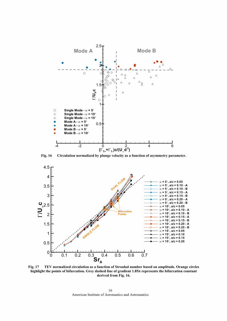
normalizing variable. Shown in Fig. 16 is this alternative circulation parameter with the same asymmetry parameter.

As expected the data points have collapsed down to a smaller band, but more importantly there is now a clear

boundary between the single and dual modes with minimal scatter of the data. The critical value of circulation

normalized by plunge velocity corresponding to the bifurcation points is Γ/UPc = 1.85. When compared to Fig. 15

the collapse of the data into a smaller band in Fig. 16 elucidates the importance of plunge velocity. This is further

emphasized in Fig. 17, which shows all the trailing-edge vortex circulations for all amplitudes and angles of attack

plotted against SrA (effectively plunge velocity). The collapse of all the data sets onto a common parabola reinforces

the significance of plunge velocity in determining the trailing-edge vortex strength. In addition this figure

demonstrates the three possible bifurcation criteria: SrA = 0.45±0.05 on the x-axis, Γ/U∞c = 2.60±0.30 on the y-axis,

and Γ/UPc = 1.85 as a straight line with its gradient determined by:

7


85.1=Γ

=Γ

∞cSrUcU AP π

therefore,

ASrcU

π85.1=Γ

∞

This line therefore passes through the points of bifurcation with the values above being dual mode and the values

below single mode. All the available data confirms the importance of this variable, however given that the data has

collapsed into a relatively small band further results are necessary to substantiate this. It has previously been

suggested27-30

that Γ/Upc can be interpreted as a dimensionless vortex formation time. This is derived from the idea

that Γ is the peak value of circulation at shedding and therefore a size quantity, and Up is the shear-layer feeding

velocity and therefore a rate of growth quantity. Using this interpretation, it is implied that the existence of dual flow

and bifurcation requires a minimum vortex formation time. To answer why will require further results and analysis.

IV. Conclusions

Experiments were performed to measure the lift force and flow field associated with small-amplitude plunging

motion of an airfoil at pre-stall, stall and post-stall angles of attack at low Reynolds numbers. For pre-stall and stall

angles of attack at larger amplitudes (a/c ≥ 0.10) it was possible to produce two entirely different flow fields with

two different values of lift coefficient at the same oscillation frequency. The mode A flow field is associated with

trailing-edge vortex pairing near the bottom of the plunge motion, resulting in an upwards deflected jet that

reinforces the upper surface leading-edge vortex and thus creates high lift. The mode B flow field is associated with

trailing-edge vortex pairing near the top of the plunge motion, resulting in a downwards deflected jet, a weak upper

surface leading-edge vortex and thus low or negative lift. The difference between the two modes was due to the

initial conditions. To produce mode A it was necessary to start with a stationary airfoil, gradually increasing the

frequency so as to create a pre-existing wake which is already inclined upwards. To produce the mode B flow field it

is necessary to impulsively start the wing at the maximum frequency.

Analysis of the trailing edge vortices lead to two parameters which describe the wake behavior. Firstly, an

asymmetry parameter is derived from the difference in circulation of the clockwise and counter-clockwise trailing-

edge vortex. This parameter determines whether the flow field is mode A or B. Secondly a strength parameter is

derived from the average of the circulations of the trailing edge vortices. This parameter can be expressed as a

minimum Strouhal number based on amplitude, or a minimum normalized circulation. It was shown that a minimum

value of the strength parameter is necessary for bifurcation to occur. The bifurcation was therefore not observed at

small amplitudes due to insufficient trailing-edge vortex strength, nor at larger angles of attack due to greater

asymmetry in the effective angle of attack causing an imbalance in the trailing-edge vortices which gives a natural

tendency for a downward deflected mode B wake.

Acknowledgments

The authors would like to acknowledge the support from an EPSRC studentship, and the RCUK Academic

Fellowship in Unmanned Air Vehicles.

V. References

1Ho, S., Nassef, H., Pornsinsirirak, N., Tai, Y.C., and Ho, C.M., "Unsteady Aerodynamics and Flow Control for Flapping Wing

Flyers," Progress in Aerospace Sciences, Vol. 39, No. 8, 2003, pp. 635-681.

2Shyy, W., Berg, M., and Ljungqvist, D., "Flapping and Flexible Wings for Biological and Micro Air Vehicles," Progress in

Aerospace Sciences, Vol. 35, No. 5, 1999, pp. 455-505.

3Pines, D.J., and Bohorquez, F., "Challenges Facing Future Micro-Air-Vehicle Development," Journal of Aircraft, Vol. 43, No.

2, 2006, pp. 290-305.

4Ellington, C.P., vandenBerg, C., Willmott, A.P., and Thomas, A.L.R., "Leading-Edge Vortices in Insect Flight," Nature, Vol.

384, No. 6610, 1996, pp. 626-630.

5Liu, H., Ellington, C.P., Kawachi, K., Van den Berg, C., and Willmott, A.P., "A Computational Fluid Dynamic Study of

Hawkmoth Hovering," Journal of Experimental Biology, Vol. 201, No. 4, 1998, pp. 461-477.

6Miller, L.A., and Peskin, C.S., "When Vortices Stick: An Aerodynamic Transition in Tiny Insect Flight," Journal of

Experimental Biology, Vol. 207, No. 17, 2004, pp. 3073-3088.

8


7Birch, J.M., and Dickinson, M.H., "The Influence of Wing-Wake Interactions on the Production of Aerodynamic Forces in

Flapping Flight," Journal of Experimental Biology, Vol. 206, No. 13, 2003, pp. 2257-2272.

8Gursul, I., Gordnier, R., and Visbal, M., "Unsteady Aerodynamics of Nonslender Delta Wings," Progress in Aerospace

Sciences, Vol. 41, No. 7, 2005, pp. 515-557.

9Taylor, G., Wang, Z., Vardaki, E., and Gursul, I., "Lift Enhancement over Flexible Nonslender Delta Wings," AIAA Journal,

Vol. 45, No. 12, 2007, pp. 2979-2993.

10Cleaver, D.J., Wang, Z.J., and Gursul, I. "Lift Enhancement on Oscillating Airfoils," 39th AIAA Fluid Dynamics Conference,

AIAA-2009-4028, AIAA, 2009.

11Visbal, M.R., "High-Fidelity Simulation of Transitional Flows Past a Plunging Airfoil," AIAA Journal, Vol. 47, No. 11, 2009,

pp. 2685-2697.

12Cleaver, D.J., Wang, Z.J., and Gursul, I. "Delay of Stall by Small Amplitude Airfoil Oscillation at Low Reynolds Numbers,"

47th AIAA Aerospace Sciences Meeting, AIAA 2009-392, AIAA, 2009.

13Jones, K.D., Dohring, C.M., and Platzer, M.F., "Experimental and Computational Investigation of the Knoller-Betz Effect,"

AIAA Journal, Vol. 36, No. 7, 1998, pp. 1240-1246.

14Lewin, G.C., and Haj-Hariri, H., "Modelling Thrust Generation of a Two-Dimensional Heaving Airfoil in a Viscous Flow,"

Journal of Fluid Mechanics, Vol. 492, 2003, pp. 339-362.

15Heathcote, S., and Gursul, I., "Jet Switching Phenomenon for a Periodically Plunging Airfoil," Physics of Fluids, Vol. 19, No.

2, 2007.

16von Ellenrieder, K.D., and Pothos, S., "Piv Measurements of the Asymmetric Wake of a Two Dimensional Heaving

Hydrofoil," Experiments in Fluids, Vol. 44, No. 5, 2008, pp. 733-745.

17Godoy-Diana, R., Marais, C., Aider, J.L., and Wesfreid, J.E., "A Model for the Symmetry Breaking of the Reverse Benard-

Von Karman Vortex Street Produced by a Flapping Foil," Journal of Fluid Mechanics, Vol. 622, 2009, pp. 23-32.

18Moffat, R.J., "Using Uncertainty Analysis in the Planning of an Experiment," Journal of Fluids Engineering-Transactions of

the ASME, Vol. 107, No. 2, 1985, pp. 173-178.

19Heathcote, S. "Flexible Flapping Airfoil Propulsion at Low Reynolds Numbers," Ph.D. Dissertation, Dept of Mechanical

Engineering, University of Bath, Bath, 2006.

20Frampton, K.D., Goldfarb, M., Monopoli, D., and Cveticanin, D. "Passive Aeroelastic Tailoring for Optimal Flapping

Wings," Proceedings of Conference on Fixed, Flapping and Rotary Wing Vehicles at Very Low Reynolds Numbers, 2000, pp.

473-482.

21Graftieaux, L., Michard, M., and Grosjean, N., "Combining Piv, Pod and Vortex Identification Algorithms for the Study of

Unsteady Turbulent Swirling Flows," Measurement Science & Technology, Vol. 12, No. 9, 2001, pp. 1422-1429.

22Morgan, C.E., Babinsky, H., and Harvey, J.K. "Vortex Detection Methods for Use with Piv and Cfd Data," 47th AIAA

Aerospace Sciences Meeting, AIAA-2009-74, AIAA, 2009.

23Sunada, S., Sakaguchi, A., and Kawachi, K., "Airfoil Section Characteristics at a Low Reynolds Number," Journal of Fluids

Engineering-Transactions of the ASME, Vol. 119, No. 1, 1997, pp. 129-135.

24Schluter, J.U. "Lift Enhancement at Low Reynolds Numbers Using Pop-up Feathers," 39th AIAA Fluid Dynamics

Conference, AIAA-2009-4195, AIAA, 2009.

25Huang, R.F., and Lin, C.L., "Vortex Shedding and Shear-Layer Instability of Wing at Low-Reynolds Numbers," AIAA

Journal, Vol. 33, No. 8, 1995, pp. 1398-1403.

26Milne-Thomson, L.M., Theoretical Hydrodynamics, 5th ed., The Macmillan Press Ltd, London, 1968.

27Rival, D., Prangemeier, T., and Tropea, C., "The Influence of Airfoil Kinematics on the Formation of Leading-Edge Vortices

in Bio-Inspired Flight," Experiments in Fluids, Vol. 46, No. 5, 2009, pp. 823-833.

28Milano, M., and Gharib, M., "Uncovering the Physics of Flapping Flat Plates with Artificial Evolution," Journal of Fluid

Mechanics, Vol. 534, 2005, pp. 403-409.

29Dabiri, J.O., "Optimal Vortex Formation as a Unifying Principle in Biological Propulsion," Annual Review of Fluid

Mechanics, Vol. 41, 2009, pp. 17-33.

30Ringuettet, M.J., Milano, M., and Gharib, M., "Role of the Tip Vortex in the Force Generation of Low-Aspect-Ratio Normal

Flat Plates," Journal of Fluid Mechanics, Vol. 581, 2007, pp. 453-468.

9


Fig. 1 Experimental setup.

Fig. 2 a) Lift coefficient as a function of angle of attack for the stationary NACA 0012 airfoil; b) time-

averaged velocity magnitude at α = 5°, α = 10°, and α = 15° for Re = 10,000.

α,°-20 -10 0 10 20

-1.0

-0.8

-0.6

-0.4

-0.2

0.2

0.4

0.6

0.8

1.0NACA 0012, Re = 10k

NACA 0012, Re = 20k

NACA 0012, Re = 30k

NACA 0012, Re = 40k

Cl

++

++

+

+

+

+

++

+

++

+

+

+ ++

+ +

Sunada et al., Re = 4k+

⊗

⊗

⊗

⊗

⊗

⊗⊗

⊗

Schluter, Re = 31k⊗

a) b)

2.0

1.5

1.0

0.5

0.0

V/U∞

α =

5°

α =

10

° α

= 1

5°

CAMERA

POSITION

OSCILLATIONS

LASER

SHEET

FREESTREAM

VELOCITY

10


Fig. 3 Lift coefficient as a function of Src for: a) α = 5°, b) α = 10°, and c) α = 15°. Increasing frequency: solid

lines and full symbols; decreasing frequency: dashed lines and open symbols.

Src

Cl

0 0.5 1 1.5 2 2.5 30

0.5

1

1.5

2

2.5

3

a/c = 0.025 - inc.

a/c = 0.025 - dec.

a/c = 0.050 - inc.

a/c = 0.050 - dec.

a/c = 0.100 - inc.

a/c = 0.100 - dec.

a/c = 0.150 - inc.

a/c = 0.150 - dec.

a/c = 0.200 - inc.

a/c = 0.200 - dec.

c)

Src

Cl

0.5 1 1.5 2 2.5 3

-2

-1

0

1

2

3

4

5

6a/c = 0.025 inc.

a/c = 0.025 dec.

a/c = 0.050 inc.

a/c = 0.050 dec.

a/c = 0.100 inc.

a/c = 0.100 dec.

a/c = 0.150 inc.

a/c = 0.150 dec.

a/c = 0.200 inc.

a/c = 0.200 dec.

a)

Src

Cl

0.5 1 1.5 2 2.5 3

-1

0

1

2

3

4

5

6a/c = 0.025 inc.

a/c = 0.025 dec.

a/c = 0.050 inc.

a/c = 0.050 dec.

a/c = 0.100 inc.

a/c = 0.100 dec.

a/c = 0.150 inc.

a/c = 0.150 dec.

a/c = 0.200 inc.

a/c = 0.200 dec.

b)

11


Fig. 4 Time-averaged velocity magnitude for a/c = 0.150, α = 5°, and: a) Src = 1.500 - pre-bifurcation, b) Src =

2.025 – mode A, and c) Src = 2.025 – mode B.

a) b) c)

2.0

1.5

1.0

0.5

0.0

V/U∞

a)

b)

c)

d)

MODE A MODE B PRE-BIFURCATION

Fig. 5 Phase-averaged vorticity contour plots for the same cases as in Fig. 4.

The points in the cycle are shown on the diagram to the left.

25

0

-25

ωc

/U∞

12


Fig. 6 Normalized peak circulation for both LEVs, and both TEVs for: a/c = 0.150, α = 5°.

Fig. 7 Phase-averaged vorticity contour plots at the top (left) and bottom (right) of the motion comparing the

mode A flowfield for a/c = 0.15, Src = 2.025 and: a) α = 5°, b) α = 10°.

Fig. 8 Phase-averaged vorticity contour plots at the top (left) and bottom (right) of the motion comparing the

mode B flowfield for a/c = 0.15, Src = 2.025 and: a) α = 5°, b) α = 10°.

Src

Γ/U

∞c

0 0.5 1 1.5 2

-5

-4

-3

-2

-1

0

1

2

3

4

5

Clockwise LEV - A

Clockwise LEV - B

Counter-Clockwise LEV - A

Counter-Clockwise LEV - B

Clockwise TEV - A

Clockwise TEV - B

Counter-Clockwise TEV - A

Counter-Clockwise TEV - B

b)

a)

100

50

0

-50

-100

ωc

/U∞

a)

b)

100

50

0

-50

-100

ωc

/U∞

13


Fig. 9 Method used to determine αvortex for the counter-clockwise TEV. It is first located in the phase-

averaged data, a line of best fit is then applied giving a gradient related to αvortex.

Fig. 10 Trailing edge vortex trajectory angle for: a) α = 5°, and b) α = 10°.

x xx

x

x

Src

αvortex,°

0.5 1 1.5 2 2.5 3

-20

-15

-10

-5

0

5

10

15

20α = 5°, a/c = 0.05

α = 5°, a/c = 0.10 - A

α = 5°, a/c = 0.10 - B

α = 5°, a/c = 0.15 - A

α = 5°, a/c = 0.15 - B

α = 5°, a/c = 0.20 - A

α = 5°, a/c = 0.20 - B

x

a)

x

xx

x

x

Src

αvortex,°

0.5 1 1.5 2 2.5 3

-20

-15

-10

-5

0

5

10

15

20α = 10°, a/c = 0.05

α = 10°, a/c = 0.10 - A

α = 10°, a/c = 0.10 - B

α = 10°, a/c = 0.15 - A

α = 10°, a/c = 0.15 - B

α = 10°, a/c = 0.20 - A

α = 10°, a/c = 0.20 - B

x

b)

2 3

4

1

14


SrA

αeff,°

0.1 0.2 0.3 0.4 0.5 0.6 0.7

-60

-40

-20

0

20

40

60

80

a/c = 0.10

a/c = 0.15

a/c = 0.20

α = 5°α = 10°α = 15°

α = 15°α = 10°α = 5°

Fig. 11 Effective angle of attack as a function of Strouhal number based on amplitude. Solid line: αeff,max,

dashed line: αeff,min. Symbols denote the point of bifurcation as determined from the force measurements.

Fig. 12 Normalized absolute circulation of the separate TEVs for a/c = 0.10 and: a) α = 5°, b) α = 10°, and

c) α = 15°.

Fig. 13 Vorticity contours showing the similarity of flowfields across different angles of attack for a/c =

0.150, Src=2.025 and: a) α = 5° - mode B, b) α = 10° - mode B, and c) α = 15°.

Src

Γ/U

∞c

0 0.5 1 1.5 2 2.5 30

1

2

3

4

Clockwise Vortex - A

Clockwise Vortex - B

Counter-Clockwise Vortex - A

Counter-Clockwise Vortex - B

a)

Src

Γ/U

∞c

0 0.5 1 1.5 2 2.5 30

1

2

3

4

Clockwise Vortex - A

Clockwise Vortex - B

Counter-Clockwise Vortex - A

Counter-Clockwise Vortex - B

b)

Src

Γ/U

∞c

0 0.5 1 1.5 2 2.5 30

1

2

3

4

Clockwise Vortex

Counter-Clockwise Vortex

c)

a) b) c)

100

50

0

-50

-100

ωc

/U∞

15


+

+

+

+

+

++

+

+

+

++

+

Src

Γ/U

∞c

0 0.5 1 1.5 2 2.5 30

0.5

1

1.5

2

2.5

3

3.5

4

4.5

α = 5°, a/c = 0.05

α = 5°, a/c = 0.10 - A

α = 5°, a/c = 0.10 - B

α = 5°, a/c = 0.15 - A

α = 5°, a/c = 0.15 - B

α = 5°, a/c = 0.20 - A

α = 5°, a/c = 0.20 - B

α = 10°, a/c = 0.05

α = 10°, a/c = 0.10 - A

α = 10°, a/c = 0.10 - B

α = 10°, a/c = 0.15 - A

α = 10°, a/c = 0.15 - B

α = 10°, a/c = 0.20 - A

α = 10°, a/c = 0.20 - B

α = 15°, a/c = 0.05

α = 15°, a/c = 0.10

α = 15°, a/c = 0.15

α = 15°, a/c = 0.20

+

+

+

Fig. 14 Average absolute TEV circulation as a function of Strouhal number.

Fig. 15 Normalized circulation as a function of asymmetry parameter.

(ΓT++Γ

T-)c/(U

∞d2)

Γ/U

∞c

-4 -2 0 2 4 6

1

2

3

4

Single Mode - α = 5°



Mode A - α = 5°

Mode A - α = 10°

Mode B - α = 5°

Mode B - α = 10°

Mode A Mode B

16


Fig. 16 Circulation normalized by plunge velocity as a function of asymmetry parameter.

Fig. 17 TEV normalized circulation as a function of Strouhal number based on amplitude. Orange circles

highlight the points of bifurcation. Grey dashed line of gradient 1.85π represents the bifurcation constant

derived from Fig. 16.

(ΓT++Γ

T-)c/(U

∞d2)

Γ/U

Pc

-4 -2 0 2 4 6

0.5

1

1.5

2

2.5




Mode A - α = 5°

Mode A - α = 10°

Mode B - α = 5°

Mode B - α = 10°

Mode A Mode B

+

+

+

+

+

++

+

+

+

++

+

SrA

Γ/U

∞c

0 0.1 0.2 0.3 0.4 0.5 0.6 0.70

0.5

1

1.5

2

2.5

3

3.5

4

4.5

α = 5°, a/c = 0.05

α = 5°, a/c = 0.10 - A

α = 5°, a/c = 0.10 - B

α = 5°, a/c = 0.15 - A

α = 5°, a/c = 0.15 - B

α = 5°, a/c = 0.20 - A

α = 5°, a/c = 0.20 - B

α = 10°, a/c = 0.05

α = 10°, a/c = 0.10 - A

α = 10°, a/c = 0.10 - B

α = 10°, a/c = 0.15 - A

α = 10°, a/c = 0.15 - B

α = 10°, a/c = 0.20 - A

α = 10°, a/c = 0.20 - B

α = 15°, a/c = 0.05

α = 15°, a/c = 0.10

α = 15°, a/c = 0.15

α = 15°, a/c = 0.20

+

+

+

SINGLEFLOW

DUALFLOW

BifurcationPoints

Documents

Vortex Mode Bifurcation and Lift Force of a Plunging ...people.bath.ac.uk/en3djc/AIAA FINAL PAPER - David Cleaver (10_01).pdf · vortex strength, nor at larger angles ... The LEV