George Kopasakis, Joseph W. Connolly, and Daniel E. PaxsonGlenn Research Center, Cleveland, Ohio

Peter MaUniversity of Florida, Gainesville, Florida

Volume Dynamics Propulsion System Modeling for Supersonics Vehicle Research

NASA/TM—2008-215172

May 2008

GT2008–50524

https://ntrs.nasa.gov/search.jsp?R=20080022415 2018-07-29T09:37:48+00:00Z

NASA STI Program . . . in Profi le

Since its founding, NASA has been dedicated to the advancement of aeronautics and space science. The NASA Scientifi c and Technical Information (STI) program plays a key part in helping NASA maintain this important role.

The NASA STI Program operates under the auspices of the Agency Chief Information Offi cer. It collects, organizes, provides for archiving, and disseminates NASA’s STI. The NASA STI program provides access to the NASA Aeronautics and Space Database and its public interface, the NASA Technical Reports Server, thus providing one of the largest collections of aeronautical and space science STI in the world. Results are published in both non-NASA channels and by NASA in the NASA STI Report Series, which includes the following report types: • TECHNICAL PUBLICATION. Reports of

completed research or a major signifi cant phase of research that present the results of NASA programs and include extensive data or theoretical analysis. Includes compilations of signifi cant scientifi c and technical data and information deemed to be of continuing reference value. NASA counterpart of peer-reviewed formal professional papers but has less stringent limitations on manuscript length and extent of graphic presentations.

• TECHNICAL MEMORANDUM. Scientifi c

and technical fi ndings that are preliminary or of specialized interest, e.g., quick release reports, working papers, and bibliographies that contain minimal annotation. Does not contain extensive analysis.

• CONTRACTOR REPORT. Scientifi c and

technical fi ndings by NASA-sponsored contractors and grantees.

• CONFERENCE PUBLICATION. Collected

papers from scientifi c and technical conferences, symposia, seminars, or other meetings sponsored or cosponsored by NASA.

• SPECIAL PUBLICATION. Scientifi c,

technical, or historical information from NASA programs, projects, and missions, often concerned with subjects having substantial public interest.

• TECHNICAL TRANSLATION. English-

language translations of foreign scientifi c and technical material pertinent to NASA’s mission.

Specialized services also include creating custom thesauri, building customized databases, organizing and publishing research results.

For more information about the NASA STI program, see the following:

• Access the NASA STI program home page at http://www.sti.nasa.gov

• E-mail your question via the Internet to help@

sti.nasa.gov • Fax your question to the NASA STI Help Desk

at 301–621–0134 • Telephone the NASA STI Help Desk at 301–621–0390 • Write to:

NASA Center for AeroSpace Information (CASI) 7115 Standard Drive Hanover, MD 21076–1320

George Kopasakis, Joseph W. Connolly, and Daniel E. PaxsonGlenn Research Center, Cleveland, Ohio

Peter MaUniversity of Florida, Gainesville, Florida

Volume Dynamics Propulsion System Modeling for Supersonics Vehicle Research

NASA/TM—2008-215172

May 2008

GT2008–50524

National Aeronautics andSpace Administration

Glenn Research CenterCleveland, Ohio 44135

Prepared for theTurbo Expo 2008 Gas Turbine Technical Congress and Expositionsponsored by the American Society of Mechanical EngineersBerlin, Germany, June 9–13, 2008

Acknowledgments

The authors would like to acknowledge Kevin J. Melcher and Clarence T. Chang from NASA Glenn for helpful discussions in the course of developing this model.

Available from

NASA Center for Aerospace Information7115 Standard DriveHanover, MD 21076–1320

National Technical Information Service5285 Port Royal RoadSpringfi eld, VA 22161

Available electronically at http://gltrs.grc.nasa.gov

Trade names and trademarks are used in this report for identifi cation only. Their usage does not constitute an offi cial endorsement, either expressed or implied, by the National Aeronautics and

Space Administration.

This work was sponsored by the Fundamental Aeronautics Program at the NASA Glenn Research Center.

Level of Review: This material has been technically reviewed by technical management.

NASA/TM—2008-215172 1

Volume Dynamics Propulsion System Modeling For Supersonics Vehicle Research

George Kopasakis, Joseph W. Connolly, and Daniel E. Paxson

National Aeronautics and Space Administration Glenn Research Center Cleveland, Ohio 44135

Peter Ma

University of Florida Gainesville, Florida 32611

Abstract

Under the NASA Fundamental Aeronautics Program the Su-personics Project is working to overcome the obstacles to super-sonic commercial flight. The proposed vehicles are long slim body aircraft with pronounced aero-servo-elastic modes. These modes can potentially couple with propulsion system dynamics; leading to performance challenges such as aircraft ride quality and stability. Other disturbances upstream of the engine gener-ated from atmospheric wind gusts, angle of attack, and yaw can have similar effects. In addition, for optimal propulsion system performance, normal inlet-engine operations are required to be closer to compressor stall and inlet unstart. To study these phe-nomena an integrated model is needed that includes both air-frame structural dynamics as well as the propulsion system dynamics. This paper covers the propulsion system component volume dynamics modeling of a turbojet engine that will be used for an integrated vehicle Aero-Propulso-Servo-Elastic model and for propulsion efficiency studies.

Nomenclature A area, m2 cp specific heat at constant pressure, J/(kg*K) cv specific heat at constant volume, J/(kg*K F thrust, N g gravitational constant, 1 (kg*m)/(N*sec2) h static enthalpy, J/kg I moment of inertial, (N*m)/sec2 J mechanical equivalent of heat, 1 (N*m)/J KA, KB combustor coefficients, unit less KC combustor coefficients, (N2*sec2)/(kg2*m4*K) Kb bleed flow coefficient, (kg*K1/2)/(N*sec) Knoz nozzle parameter, (kg*m2*K1/2)/(N*sec) l length, m M mach number Mair molecular weight of air, 0.02897 (kg/mol) Mfuel molecular weight of fuel (JP-4), 0.139 (kg/mol) Mca molecular weight of cooling air, 0.02897 (kg/mol) N rotational speed, rpm Nc corrected speed ratio P pressure, N/m2 Pr pressure ratio

R universal gas constant, 287 (N*m)/(kg*K) r rotor mean radius, m rT rotor tip radius, m T temperature, K U velocity, m/sec Uab volumetric flow rate of combustor air, m/sec V volume, m3 .W mass flow rate, kg/sec

.cmfW corrected mass flow rate, kg/sec .''fW externally acted upon fuel flow, kg/sec

Greek

γ ratio of specific heats, γcp = 1.4, γcb = γtb = γab = 1.31 η efficiency Θ molecular vibration energy constant associated with a

gas mixture, K ρ weight density, kg/m3 τ delay time τt delay time associated with fuel transport and mixing φ fuel to air ratio

Subscripts a variable associated with combustor acoustics ab variable associated with the afterburner amb variable associated with ambient conditions b variable associated with compressor bleed c variable associated with stage characteristics ca variable associated with cooling air cb variable associated with the combustor cp variable associated with the compressor d variable associated with designed value e variable associated with engine exit condition f variable associated with fuel fl variable associated with flame dynamics i index associated with nozzle volume element number j index associated with turbine stage number k number of compressor stages l index associated with inlet volume element number m number of turbine stages n index associated with compressor stage number noz variable associated with the nozzle

NASA/TM—2008-215172 2

o variable associated with engine entrance condition q number of inlet volume elements perf variable associated with a thermally perfect gas ref variable associated with reference value tb variable associated with the turbine s static condition sv static condition variable associated with stage volume tc total condition variable associated with stage charac-

teristics tv total condition variable associated with stage volume z variable associated with nozzle

Introduction In many aero-propulsion applications a relatively low fidelity

engine model (i.e., without volume dynamics), which includes speed and temperature dynamics with the appropriate component performance characteristics is adequate to design control laws. The actuation system, such as fuel actuation, is rather slow and as a result the control bandwidth is reduced, which makes such lower fidelity simulations (refs. 1 and 2) appropriate for controls design. In supersonics, the slim body structure of the vehicle excites structural dynamics, which can introduce upstream flow field disturbances at higher frequencies (up to 50 Hz or more). The vehicle control surfaces are actuated to suppress some of these structural modes associated with flutter (refs. 3 and 4).

Analysis needs to be carried out to understand how these aero-servo-elastic (ASE) excitations as well as other atmospheric disturbances impact the propulsion system in terms of thrust variations that can affect ride quality and vehicle stability. In addition, the coupling of the propulsion system to the vehicle ASE modes needs to be analyzed, and for that an integrated aero-propulso-servo-elastic system (APSE) simulation is needed. Due to the high frequencies of these modes the propulsion system simulation needs to incorporate 1D volume dynamics based on conservation equations modeling.

A propulsion system for a supersonic vehicle also differs from a conventional vehicle in that a supersonic vehicle utilizes a su-personic inlet with active controls for shock positioning, which can also excite higher frequency dynamics. In addition, how these upstream disturbances impact the inlet shock positioning, pres-sure recovery, as well as inlet distortion and its impact on thrust variations also needs to be analyzed. Also to achieve high per-formance, a supersonic vehicle would operate closer to compres-sor stall and inlet unstart. This necessitates modeling utilizing component volume dynamics in order to study the dynamic inter-action of these engine components. This paper covers the propul-sion system component volume dynamics modeling of a turbojet engine. The supersonic inlet dynamics and their effect on the rest of the propulsion system and the vehicle will be addressed in some future studies.

The propulsion system simulation described in this paper uses the architecture of a J85-13 turbojet engine; although it can be adapted to simulate different engines due to its generic architec-ture. The development of this engine simulation in MATLAB SIMULINK®

is partially based on a simulation developed years

ago at NASA Glenn Research Center (GRC) (ref. 5), using an analog computer and also referred herein as the Seldner simula-tion. In the engine simulation described here, some of the geome-tries are approximated, and the component performance maps are generic. The Seldner simulation was verified in both steady-state and dynamic modes by comparing analytical results with experi-mental data obtained from tests performed at GRC with a J85-13 engine. The simulation described in this paper has been verified by comparing it against simulation results provided in Seldner (ref. 5), and also from simulations that display expected engine responses based on experience.

The engine model presented is based on stage-by-stage com-ponent volume dynamics. The simulation results presented are based on component level volume dynamics. The component level volume dynamics model of the engine is envisioned to be a stepping stone towards eventually obtaining a stage-by-stage model with all the appropriate stage performance maps that may be required to address the thrust variations issue.

The paper is organized as follows. First, the engine dynamic model development is described in detail for each major compo-nent. This is followed by some simulation results to help verify the engine simulation, as well some preliminary thrust variation studies. Finally, future plans for upgrading the engine model, including plans for additional analysis and controls design are discussed, followed by concluding remarks.

Engine Model The Seldner (ref. 5) simulation technique was applied to the

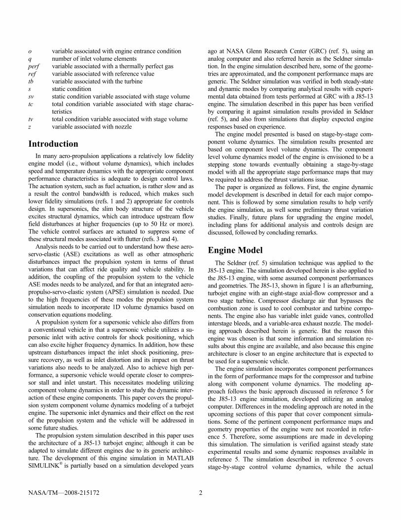
J85-13 engine. The simulation developed herein is also applied to the J85-13 engine, with some assumed component performances and geometries. The J85-13, shown in figure 1 is an afterburning, turbojet engine with an eight-stage axial-flow compressor and a two stage turbine. Compressor discharge air that bypasses the combustion zone is used to cool combustor and turbine compo-nents. The engine also has variable inlet guide vanes, controlled interstage bleeds, and a variable-area exhaust nozzle. The model-ing approach described herein is generic. But the reason this engine was chosen is that some information and simulation re-sults about this engine are available, and also because this engine architecture is closer to an engine architecture that is expected to be used for a supersonic vehicle.

The engine simulation incorporates component performances in the form of performance maps for the compressor and turbine along with component volume dynamics. The modeling ap-proach follows the basic approach discussed in reference 5 for the J85-13 engine simulation, developed utilizing an analog computer. Differences in the modeling approach are noted in the upcoming sections of this paper that cover component simula-tions. Some of the pertinent component performance maps and geometry properties of the engine were not recorded in refer-ence 5. Therefore, some assumptions are made in developing this simulation. The simulation is verified against steady state experimental results and some dynamic responses available in reference 5. The simulation described in reference 5 covers stage-by-stage control volume dynamics, while the actual

NASA/TM—2008-215172 3

Figure 1.—J85-13 engine.

simulation here is incorporated with component level lumped volume dynamics, and therefore, there could be some differ-ences in dynamic responses.

Compressor This section describes the compressor model based on the

individual compressor stages. In reference 5 the compressor maps were expressed in terms of normalized coefficients of pressure and temperature versus flow. Because it is rare at present to find performance maps expressed in these terms, a map generation routine is used to derive overall compressor maps in a more conventional form consisting of the pressure ratio versus corrected mass flow rate and compressor effi-ciency versus pressure ratio. The compressor maps would normally differ for inlet guide vane position and bleed flow. Certain geometrical properties of the compressor like cross section area, length, mean radius, and tip radius are not avail-able and are estimated.

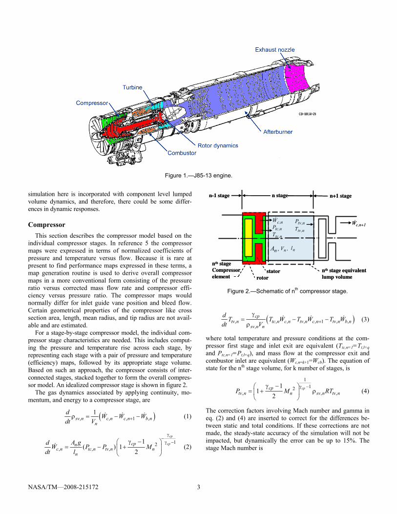
For a stage-by-stage compressor model, the individual com-pressor stage characteristics are needed. This includes comput-ing the pressure and temperature rise across each stage, by representing each stage with a pair of pressure and temperature (efficiency) maps, followed by its appropriate stage volume. Based on such an approach, the compressor consists of inter-connected stages, stacked together to form the overall compres-sor model. An idealized compressor stage is shown in figure 2.

The gas dynamics associated by applying continuity, mo-mentum, and energy to a compressor stage, are

( ), , , 1 ,1

sv n c n c n b nn

d W W Wdt V +ρ = − − (1)

12

, , ,1

( ) 12

cp

cpcpnc n tc n tv n n

n

A gd W P P Mdt l

γ−γ −γ −⎛ ⎞

= − +⎜ ⎟⎝ ⎠

(2)

n+1 stage

1n,cW +n,cWn,tcP

n,tvP

n,tcTn,tvT

,Vn,An nl

n-1 stage n stage

nth stage equivalentlump volume

nth stageCompressor element rotor

stator

n+1 stage

1n,cW +n,cWn,tcP

n,tvP

n,tcTn,tvT

,Vn,An nl

n-1 stage n stage

nth stage equivalentlump volume

nth stageCompressor element rotor

stator

Figure 2.—Schematic of nth compressor stage.

( ), , , , , 1 , ,,

cptv n tc n c n tv n c n tv n b n

sv n n

d T T W T W T Wdt V +

γ= − −ρ

(3)

where total temperature and pressure conditions at the com-pressor first stage and inlet exit are equivalent (Ttc,n=1=Tt,l=q and Ptc,n=1=Pt,l=q), and mass flow at the compressor exit and combustor inlet are equivalent (Wc,n=k+1=Wcb). The equation of state for the nth stage volume, for k number of stages, is

112

, , ,1

12

cpcptv n n sv n tv nP M RT

γ −γ −⎛ ⎞= + ρ⎜ ⎟⎝ ⎠

(4)

The correction factors involving Mach number and gamma in eq. (2) and (4) are inserted to correct for the differences be-tween static and total conditions. If these corrections are not made, the steady-state accuracy of the simulation will not be impacted, but dynamically the error can be up to 15%. The stage Mach number is

NASA/TM—2008-215172 4

,

, ,

c nn

sv n n cp s n

WM

A RT=ρ γ

(5)

where

2,

, , 2 2, ,2

c ns n tv n

sv n n p n

WT T

A c= −

ρ (6)

Bleed flow is extracted from some of the compressor stages. The bleed flow relation assumes choked flow condi-tions, were Kb, is the portion of the bleed flow effective area.

,, ,

,

tv nb n b b n

tv n

PW K A

T= (7)

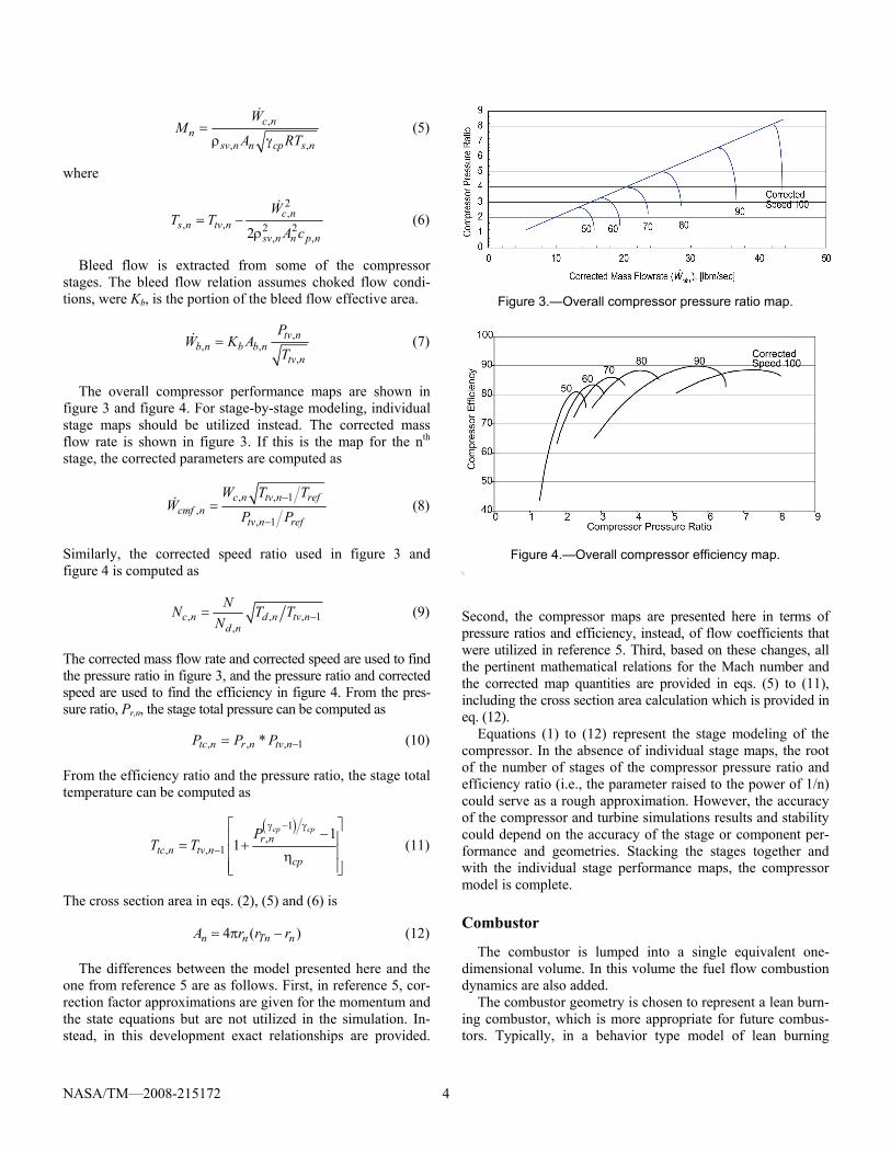
The overall compressor performance maps are shown in figure 3 and figure 4. For stage-by-stage modeling, individual stage maps should be utilized instead. The corrected mass flow rate is shown in figure 3. If this is the map for the nth stage, the corrected parameters are computed as

, , 1,

, 1

c n tv n refcmf n

tv n ref

W T TW

P P−

−= (8)

Similarly, the corrected speed ratio used in figure 3 and figure 4 is computed as

, , , 1,

c n d n tv nd n

NN T TN −= (9)

The corrected mass flow rate and corrected speed are used to find the pressure ratio in figure 3, and the pressure ratio and corrected speed are used to find the efficiency in figure 4. From the pres-sure ratio, Pr,n, the stage total pressure can be computed as

1,,, * −= ntvnrntc PPP (10)

From the efficiency ratio and the pressure ratio, the stage total temperature can be computed as

( )1,

, , 11

1cp cp

r ntc n tv n

cp

PT T

γ − γ

−

⎡ ⎤−⎢ ⎥= +⎢ ⎥η⎢ ⎥⎣ ⎦

(11)

The cross section area in eqs. (2), (5) and (6) is

4 ( )n n Tn nA r r r= π − (12)

The differences between the model presented here and the one from reference 5 are as follows. First, in reference 5, cor-rection factor approximations are given for the momentum and the state equations but are not utilized in the simulation. In-stead, in this development exact relationships are provided.

Figure 3.—Overall compressor pressure ratio map.

Figure 4.—Overall compressor efficiency map.

\\

Second, the compressor maps are presented here in terms of pressure ratios and efficiency, instead, of flow coefficients that were utilized in reference 5. Third, based on these changes, all the pertinent mathematical relations for the Mach number and the corrected map quantities are provided in eqs. (5) to (11), including the cross section area calculation which is provided in eq. (12).

Equations (1) to (12) represent the stage modeling of the compressor. In the absence of individual stage maps, the root of the number of stages of the compressor pressure ratio and efficiency ratio (i.e., the parameter raised to the power of 1/n) could serve as a rough approximation. However, the accuracy of the compressor and turbine simulations results and stability could depend on the accuracy of the stage or component per-formance and geometries. Stacking the stages together and with the individual stage performance maps, the compressor model is complete.

Combustor

The combustor is lumped into a single equivalent one-dimensional volume. In this volume the fuel flow combustion dynamics are also added.

The combustor geometry is chosen to represent a lean burn-ing combustor, which is more appropriate for future combus-tors. Typically, in a behavior type model of lean burning

NASA/TM—2008-215172 5

combustors (ref. 6), the combustion dynamics can be modeled as a self excitation system of a first order transfer function (TF) representing the flame dynamics, with a second order undamped TF representing the acoustics. But the acoustics here are represented with a first order TF. The assumption is that the unsteady combustion typical to lean burning combus-tors will be mitigated by some control approach like the one described in (ref. 6). The total combustion time delay is the sum of the delays of fuel transport and mixing, the flame dy-namics, and the acoustics as

cb t fl aτ = τ + τ + τ (13)

Given a combustor volume, Vcb, and a volumetric flow rate through the combustor, Ucb, the combustor time delay can be approximated as

cb cb cbV Uτ = (14)

The total combustion time delay is assumed to be in the order of 5 msec, with the fuel transport and mixing time delay ac-counting for the greater part of this delay. The overall fuel flow combustion dynamics are modeled as follows

)1)(1(

''

+τ+τ=

τ−

ssKe

W

W

afl

s

f

f t (15)

where K is a proportional TF gain, set to one. The combustor gas dynamics for continuity, momentum,

and energy are

( )", , 1

1s cb cb f c j

cb

d W W Wdt V =ρ = + − (16)

( ).

, , ,cb

cb tv n k t cb t cbcb

A gd W P P Pdt l == − − Δ (17)

'', , , , , 1

,

'',

,

cbt cb tv n k cb f t cb t cb c j

s cb cb

cbf c cb

p cb

d T T W W T T Wdt V

W hc

= =

⎛γ⎜= + −⎜ρ ⎝

⎞η⎟+⎟⎠

(18)

and the equation of state is

, , ,t cb s cb cb t cbP R T= ρ (19)

( )1cb

air fuel

RRM M

=− φ + φ

(20)

where a fuel/air ratio, φ, of about 0.02 was used that represents lean type combustion. Unlike the compressor, correction fac-

tors are not used in the combustor simulation due to the low Mach number in the combustor, which makes a negligible difference. The cp value in eq. (18) is not constant in the upper temperature range of the combustor, and for more accurate calculations eq. (44) that is provided later can be used.

In this development, hc was assumed to be a constant of 42.8e6 [J/kg] for JP-4 fuel, at about 1000 K (ref. 7). The com-bustor efficiency map (ref. 5), is shown in figure 5, where

, , ,t cb t cb tv n kT T T =Δ = − (21)

The pressure drop across the combustor is

( )2

, , ,,

C cbt cb A tv n k B t cb

tv n k

K WP K T K T

P ==

Δ = + (22)

where KA and KB are experimentally determined; KA is found from non-combustion flow tests; KB from combustion flow test. The proportionality constant, KC, is found by solving eq. (22) for KC, given the designed steady-state quantities in eq. (22) at different speeds. A table is provided in reference 5 for these values. Typical values for ΔPt,cb range from 0.05 to 0.1. In reference 5, KC has the same units as KA and KB, but KA and KB should be dimensionless.

The differences between the combustor model presented here and the Seldner model, reference 5, are as follows. First, the time delays in eqs. (13) to (15) are chosen for lean burning combustors and the relation of the overall combustor time delay, eq. (14), is provided here. Second, the equation of state is given here, where the specific gas constant is formulated for the combustion mixture. Third, the enthalpy, hc, was used as a constant here of about 1000 K. In the Seldner model, hc was determined using stage characteristics with the independent variable Tt,cb. Fourth, a correction is made to eq. (22) here that involves cbW computed from the combustor volume dynamics instead of the mass flow rate coming from the compressor.

Equations (13) through (22) complete the combustor model.

Figure 5.—Combustor efficiency representation.

NASA/TM—2008-215172 6

Turbine

In the Seldner model, reference 5, the entire turbine is mod-eled as a single lumped volume. Moreover, the turbine is combined with the non-combusting afterburner and the nozzle. This combined model was the result of having the turbine contributing to the energy conservation through the enthalpy change, the afterburner contributing to the momentum by dominating the total volume, and both the turbine and the afterburner sharing the continuity equation, with the nozzle governed by compressible flow and choked flow conditions. While the model in reference 5 may exhibit sufficient steady-state accuracy, it’s not anticipated that dynamically the fre-quencies of these components will be accurately represented. Therefore, the turbine and the subsequent afterburner models are different than those presented in reference 5.

An idealized turbine stage would be similar to the compressor stage shown in figure 2. The gas dynamics associated by applying continuity, momentum, and energy to a turbine stage are

. . .

, , 1,1 ( )c j ca c jsv j

j

d W W Wdt V

+ρ = + − (23)

. 12, , ,

1( ) 12

tb

tbj tbc j tc j tv j j

j

A gd W P P Mdt l

γ−γ −γ −⎛ ⎞= − +⎜ ⎟

⎝ ⎠ (24)

( ), , , , , , , 1,

tbtv j tc j c j t ca ca j tv j c j

sv j j

d T T W T W T Wdt V +

γ= + −ρ

(25)

where total temperature and pressure conditions at the turbine first stage and combustor exit are equivalent (Ttc,j=1=Tt,cb and Ptc,j=1=Pt,cb), and mass flow at the turbine exit and afterburner inlet are equivalent ( , 1c j m abW W= + = ). The equation of state for the jth stage volume is (for m-number of stages)

n,tvtbn,sv1tb

12

jtb

j,tv TRM2

11P ρ

γ γ −⎟⎠

⎞⎜⎝

⎛ −+= (26)

where

(1 )( )tb

air ca fuel

RRM M M

=− φ + + φ

(27)

and

,

, ,

c jj

sv j j tb tb s j

WM

A R T=ρ γ

(28)

2,

, , 2 2, ,2

c js j tv j

sv j j p j

WT T

A c= −

ρ (29)

Figure 6.—Overall turbine pressure ratio map.

Figure 7.—Overall turbine efficiency map.

The cp value in eq. (29) is not constant in the upper tempera-ture range of the turbine, and for more accurate calculations eq. (44) that is provided later can be used.

Performance maps are incorporated in this development that are more readily available, such as the ones shown in figure 6 and figure 7 for the overall turbine pressure ratio and efficiency.

The corrected mass flow rate and speed ratio are used in figure 6 and figure 7. If these are the maps for the jth stage, the corrected parameters would be computed as

ref1j,tv

ref1j,tvj,cj,cmf

.

P/P

T/TWW

−

−= (30)

1j,tvj,dj,d

j,c T/TN

NN −= (31)

From the pressure ratio, Pr,j, the stage total pressure can be computed as

jrjtvjtc PPP ,1,, −= (32)

From the efficiency ratio and the pressure ratio the stage total temperature can be computed as

11

, ,, 1

1 1 1tb

tbtc j tb r j

tv jT P

T

−γ −γ

−

⎡ ⎤⎛ ⎞⎢ ⎥⎜ ⎟= − η −⎢ ⎥⎜ ⎟⎜ ⎟⎢ ⎥⎝ ⎠⎣ ⎦

(33)

NASA/TM—2008-215172 7

The cross section area in eqs. (24), (28) and (29) is

4 ( )j j Tj jA r r r= π − (34)

Equations (23) to (34) represent the stage modeling of the turbine. Stacking the stages together and with the individual stage performance maps, the turbine model is complete.

Afterburner and Nozzle

A combined combusting afterburner and exhaust nozzle model is presented here, with the assumption that a supersonic cruise vehicle would likely employ an afterburner. It is assumed here that the large afterburner acts as a large filter, attenuating high frequency upstream disturbances, such that a detailed multi-finite element volume nozzle model will not impact dy-namic thrust calculations. With this assumption, in the com-bined model the afterburner volume dominates. Also, unlike the Seldner model, a combusting afterburner is modeled here, which also allows for temperature changes across the after-burner. Like the Seldner model, the nozzle is considered as a variable area compressible flow passage capable of choking.

Based on these assumptions, and by separating the after-burner from the turbine model as discussed in the turbine section, the gas dynamics associated by applying continuity, momentum, and energy to the afterburner and nozzle are

)(1 .,

., zabfuelab

ababs WWW

Vdtd

−+=ρ (35)

12, ,

1( ) 1

2

ab

abab abab tv j m t ab ab

ab

A gd W P P Mdt l

γ−γ −

=γ −⎛ ⎞= − +⎜ ⎟

⎝ ⎠ (36)

, , ,,

( )abt ab tv j m ab ab t ab z

s ab ab

d T T W Q T Wdt V =

γ= + −ρ

(37)

At some future point, the heat addition Qab will be consisting of two terms, similar to the combustor model. One term will be due to the heat addition of the afterburner fuel, and the other term will be due to the heat addition of the combusted fuel mixture with the associated fuel system dynamics. The equation of state is

ab,tabab,s1ab

12

abab

ab,t TRM2

11P ργ γ −

⎟⎠

⎞⎜⎝

⎛ −+= (38)

where Rab can be calculated similarly to eq. (20). The nozzle, with its mass flow rate, becomes the terminal boundary of the turbojet as

1 1

, , ,

, ,,1

ab

ab abz t ab s amb s ambz

t ab t abt ab

K P P PW

P PT

γ −γ γ⎛ ⎞ ⎛ ⎞

= −⎜ ⎟ ⎜ ⎟⎜ ⎟ ⎜ ⎟⎝ ⎠ ⎝ ⎠

(39)

The second and third multiplicative terms in eq. (39) represent the well known compressible flow function (ref. 5). The pa-rameter Kz is variable and proportional to the nozzle area. It represents the turbojet terminal impedance, and lumps the nozzle flow coefficient and nozzle area with other flow pa-rameters. This parameter, through the variable nozzle area, is scheduled as a function of engine speed to match the steady-state operating line. In the simulation, Kz was experimentally determined to better match expected results.

Equations (35) to (39) complete the afterburner and the nozzle model.

Rotor Dynamics The steady-state performance of a turbojet engine matches

the compressor with that of the turbine operating points. A mismatch in these components produces an unbalanced torque or acceleration, which is integrated through the dynamic rela-tions to seek a new steady-state match. The rotor dynamics are based on the changes of mass and enthalpy. Therefore, the change of rotor speed is a function of the energy differential between the work extracted by the turbine and the work done by the compressor a

( )( )

2

, 1

, , 1 1

30c j cb ca ca ab j m

c n k n k b b c n n

d JN W h W h W hdt NI

W h W h W h

= =

= = = =

⎛ ⎞ ⎡= + −⎜ ⎟ ⎣π⎝ ⎠⎤− + − ⎦

(40)

The enthalpies in eq. (40) can be computed as follows.

cb,tcb,pcb Tch = (41)

j,tvj,pj Tch = (42)

n,tvn,pn Tch = (43)

The specific heat at constant pressure, cp, is not constant and it varies as a function of temperature and gas mixture based on the following equation, for a thermally perfect gas.

,

,

2 /

, / 2,

1( ) 1

( 1)

x t x

x t x

Tperf x

p x p perf Tperf t x

ec cT e

θ

θ

⎧ ⎫⎡ ⎤γ − ⎛ ⎞Θ⎪ ⎪⎢ ⎥= + ⎜ ⎟⎨ ⎬⎜ ⎟⎢ ⎥γ −⎪ ⎪⎝ ⎠⎣ ⎦⎩ ⎭

(44)

The combustor and the turbine specific heat vary some in the order of 1000 K. But the specific heat will be different due to the addition of fuel. For a pure air mixture, Θ = 3056 K.

The differences between the rotor model presented here and the Seldner model, reference 5, are as follows. First, the Seld-ner model does not take into account the cooling air coming in the turbine. Second, in the Seldner model the enthalpies are not defined, and third, that model assumes a constant specific heat.

NASA/TM—2008-215172 8

Engine Thrust

Thrust was not included in the Seldner model, but it is esti-mated in this model as follows. In general, the net thrust is the sum of the momentum thrust and the pressure thrust as

,( ) ( )ze o e s amb e

WF U U P P Ag

= − + − (45)

and

1

,1

1(1 )

z

zze t ab

z zP P

γγ −⎡ ⎤− γ

= +⎢ ⎥η + γ⎣ ⎦ (46)

At steady-state, the engine thrust is primarily due to the momen-tum thrust; the pressure difference in eq. (45) is about zero by scheduling Kz (i.e., by adjusting the nozzle exit area) as a function of the speed, N. However, in the dynamic sense, for thrust calcu-lations, the pressure thrust in eq. (45) could be significant.

Engine Simulation Results In this section, selected results are presented for the whole

engine simulation running together at sea level static flight conditions. These are for the component level lumped volume dynamics engine model. All it takes to convert the compressor and turbine models presented earlier into component level lumped volumes is to drop the subscripts that represent the stage-by-stage model and also use the performance maps for the entire component. Some of the initial objectives are to analyze thrust variations and controls designs using the com-ponent level lumped volume dynamic model, and later to address whether a more detail model is needed that employs stage-by-stage volume dynamics.

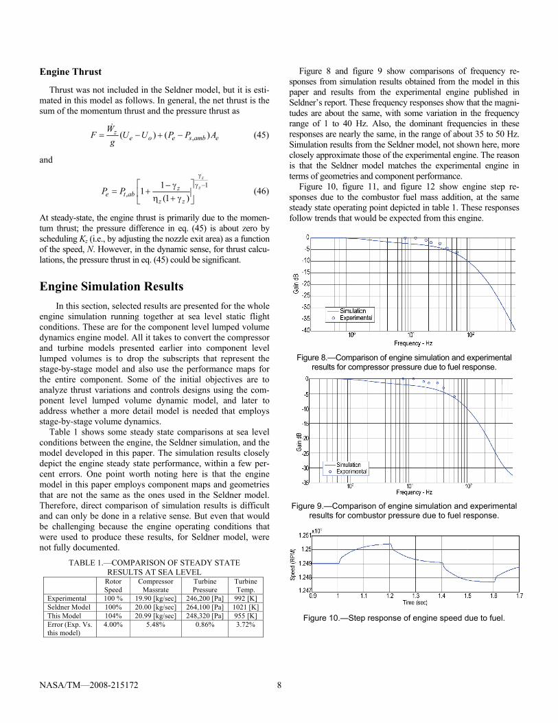
Table 1 shows some steady state comparisons at sea level conditions between the engine, the Seldner simulation, and the model developed in this paper. The simulation results closely depict the engine steady state performance, within a few per-cent errors. One point worth noting here is that the engine model in this paper employs component maps and geometries that are not the same as the ones used in the Seldner model. Therefore, direct comparison of simulation results is difficult and can only be done in a relative sense. But even that would be challenging because the engine operating conditions that were used to produce these results, for Seldner model, were not fully documented.

TABLE 1.—COMPARISON OF STEADY STATE RESULTS AT SEA LEVEL

Rotor Speed

Compressor Massrate

Turbine Pressure

Turbine Temp.

Experimental 100 % 19.90 [kg/sec] 246,200 [Pa] 992 [K] Seldner Model 100% 20.00 [kg/sec] 264,100 [Pa] 1021 [K] This Model 104% 20.99 [kg/sec] 248,320 [Pa] 955 [K] Error (Exp. Vs. this model)

4.00% 5.48% 0.86% 3.72%

Figure 8 and figure 9 show comparisons of frequency re-sponses from simulation results obtained from the model in this paper and results from the experimental engine published in Seldner’s report. These frequency responses show that the magni-tudes are about the same, with some variation in the frequency range of 1 to 40 Hz. Also, the dominant frequencies in these responses are nearly the same, in the range of about 35 to 50 Hz. Simulation results from the Seldner model, not shown here, more closely approximate those of the experimental engine. The reason is that the Seldner model matches the experimental engine in terms of geometries and component performance.

Figure 10, figure 11, and figure 12 show engine step re-sponses due to the combustor fuel mass addition, at the same steady state operating point depicted in table 1. These responses follow trends that would be expected from this engine.

Figure 8.—Comparison of engine simulation and experimental

results for compressor pressure due to fuel response.

Figure 9.—Comparison of engine simulation and experimental

results for combustor pressure due to fuel response.

Figure 10.—Step response of engine speed due to fuel.

NASA/TM—2008-215172 9

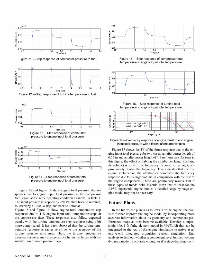
Figure 11.—Step response of combustor pressure to fuel.

Figure 12.—Step response of turbine temperature to fuel.

Figure 13.—Step response of combustor pressure to engine input total pressure.

Figure 14.—Step response of turbine total

pressure to engine input total pressure.

Figure 13 and figure 14 show engine total pressure step re-

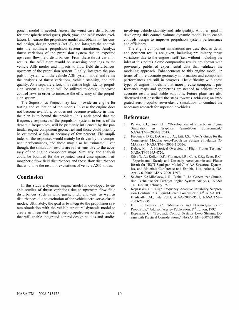
sponses due to engine input total pressure at the compressor face, again at the same operating condition as shown in table 1. The input pressure is stepped by 250 Pa, then back to nominal, followed by a –250 Pa step, and back to nominal. Figure 15 and figure 16 show engine total temperature step responses due to 1 K engine input total temperature steps at the compressor face. These responses also follow expected trends, with the turbine temperature step response being a bit more complicated. It has been observed that the turbine tem-perature response is rather sensitive to the accuracy of the turbine pressure ratio map. Thus, the turbine temperature transient response may change somewhat in the future with the substitution of more precise maps.

Figure 15.—Step response of compressor total temperature to engine input total temperature.

Figure 16.—Step response of turbine total

temperature to engine input total temperature.

Figure 17.—Frequency response of engine thrust due to engine

input total pressure with different afterburner lengths.

Figure 17 shows the TF of the thrust response due to the en-gine input total pressure for two cases; an afterburner length of 0.75 m and an afterburner length of 1.5 m (nominal). As seen in this figure, the effect of halving the afterburner length (halving its volume) is to shift the frequency response to the right, ap-proximately double the frequency. This indicates that for this engine architecture, the afterburner dominates the frequency response due to its large volume in comparison with the rest of the engine components. These are preliminary results. But if these types of trends hold, it could mean that at least for the APSE supersonic engine studies a detailed stage-by-stage en-gine model may not be necessary.

Future Plans In the future, the plan is as follows. For the engine, the plan

is to further improve the engine model by incorporating more accurate information about its geometry and component per-formance maps as they become available. Develop a super-sonic inlet 1-D finite element model in MATLAB that can be integrated to the rest of the engine simulation to arrive at an end-to-end integrated propulsion system simulation. Run analysis to find out whether a component level lumped volume dynamic model is accurate enough or if a stage-by-stage com-

NASA/TM—2008-215172 10

ponent model is needed. Assess the worst case disturbances for atmospheric wind gusts, pitch, yaw, and ASE modes exci-tation. Linearize the propulsion model and obtain TF for con-trol design, design controls (ref. 8), and integrate the controls into the nonlinear propulsion system simulation. Analyze thrust variations of the propulsion system due to expected upstream flow field disturbances. From these thrust variation results, the ASE team would be assessing couplings to the vehicle ASE modes and impacts to flow field disturbances, upstream of the propulsion system. Finally, integrate the pro-pulsion system with the vehicle ASE system model and refine the analyses of thrust variations, vehicle stability, and ride quality. As a separate effort, this relative high fidelity propul-sion system simulation will be utilized to design improved control laws in order to increase the efficiency of the propul-sion system.

The Supersonics Project may later provide an engine for testing and validation of the models. In case the engine does not become available, or does not become available in time, the plan is to bound the problem. It is anticipated that the frequency responses of the propulsion system, in terms of the dynamic frequencies, will be primarily influenced by the par-ticular engine component geometries and those could possibly be estimated within an accuracy of few percent. The ampli-tudes of the responses would mainly be driven by the compo-nent performances, and these may also be estimated. Even though, the simulation results are rather sensitive to the accu-racy of the engine component maps. Similarly, the analysis could be bounded for the expected worst case upstream at-mospheric flow field disturbances and those flow disturbances that would be the result of excitations of vehicle ASE modes.

Conclusion In this study a dynamic engine model is developed to en-

able studies of thrust variations due to upstream flow field disturbances, such as wind gusts, pitch, and yaw, as well as disturbances due to excitation of the vehicle aero-servo-elastic modes. Ultimately, the goal is to integrate the propulsion sys-tem simulation with the vehicle structural dynamic model to create an integrated vehicle aero-propulso-servo-elastic model that will enable integrated control design studies and studies

involving vehicle stability and ride quality. Another, goal in developing this control volume dynamic model is to enable controls design to improve propulsion system performance and efficiency.

The engine component simulations are described in detail and pertinent results are given, including preliminary thrust variations due to the engine itself (i.e., without including the inlet at this point). Some comparative results are shown with previously published experimental data that validates the modeling approach. Enhancements to this engine model, in terms of more accurate geometry information and component performances are still in progress. The difficulty with these types of engine models is that more precise component per-formance maps and geometries are needed to achieve more accurate results and stable solutions. Future plans are also discussed that described the steps towards achieving an inte-grated aero-propulso-servo-elastic simulation to conduct the necessary research for supersonic vehicles.

References 1. Parker, K.I.; Guo, T.H.: “Development of a Turbofan Engine

Simulation in Graphical Simulation Environment,” NASA/TM—2003-212543.

2. Frederick, D.K.; DeCastro, J.A.; Litt, J.S.: “User’s Guide for the Commercial Modular Aero-Propulsion System Simulation (C-MAPPS),” NASA/TM—2007-215026.

3. Kehoe, M.: “A Historical Overview of Flight Flutter Testing,” NASA/TM-1995-4720.

4. Silva W.A.; Keller, D.F.; Florance, J.R.; Cole, S.R.; Scott, R.C.: “Experimental Steady and Unsteady Aerodynamic and Flutter Result for HSCT Semispan Models,” AIAA Structural Dynam-ics, and Materials Conference and Exhibit, 41st, Atlanta, GA, Apr. 3-6, 2000, AIAA–2000–1697.

5. Seldner, K.; Mihaloew, J. R.; Blaha, R. J.: “Generalized Simula-tion Technique for Turbojet Engine System Analysis,” NASA TN D–6610, February 1972.

6. Kopasakis, G.: “High Frequency Adaptive Instability Suppres-sion Controls in a Liquid-Fueled Combustor,” 39th AIAA JPC, Huntsville, AL, July 2003, AIAA–2003–9581, NASA/TM—2003-212535.

7. Hill, P.; Peterson, C.: “Mechanics and Thermodynamics of Propulsion,” Addison Wesley Publication, 2nd Edition, 1992.

8. Kopasakis G.: “Feedback Control Systems Loop Shaping De-sign with Practical Considerations,” NASA/TM—2007-215007.

REPORT DOCUMENTATION PAGE Form Approved OMB No. 0704-0188

The public reporting burden for this collection of information is estimated to average 1 hour per response, including the time for reviewing instructions, searching existing data sources, gathering and maintaining the data needed, and completing and reviewing the collection of information. Send comments regarding this burden estimate or any other aspect of this collection of information, including suggestions for reducing this burden, to Department of Defense, Washington Headquarters Services, Directorate for Information Operations and Reports (0704-0188), 1215 Jefferson Davis Highway, Suite 1204, Arlington, VA 22202-4302. Respondents should be aware that notwithstanding any other provision of law, no person shall be subject to any penalty for failing to comply with a collection of information if it does not display a currently valid OMB control number. PLEASE DO NOT RETURN YOUR FORM TO THE ABOVE ADDRESS. 1. REPORT DATE (DD-MM-YYYY) 01-05-2008

2. REPORT TYPE Technical Memorandum

3. DATES COVERED (From - To)

4. TITLE AND SUBTITLE Volume Dynamics Propulsion System Modeling For Supersonics Vehicle Research

5a. CONTRACT NUMBER

5b. GRANT NUMBER

5c. PROGRAM ELEMENT NUMBER

6. AUTHOR(S) Kopasakis, George; Connolly, Joseph, W.; Paxson, Daniel, E.; Ma, Peter

5d. PROJECT NUMBER

5e. TASK NUMBER

5f. WORK UNIT NUMBER WBS 984754.02.07.03.20.02

7. PERFORMING ORGANIZATION NAME(S) AND ADDRESS(ES) National Aeronautics and Space Administration John H. Glenn Research Center at Lewis Field Cleveland, Ohio 44135-3191

8. PERFORMING ORGANIZATION REPORT NUMBER E-16415

9. SPONSORING/MONITORING AGENCY NAME(S) AND ADDRESS(ES) National Aeronautics and Space Administration Washington, DC 20546-0001

10. SPONSORING/MONITORS ACRONYM(S) NASA

11. SPONSORING/MONITORING REPORT NUMBER NASA/TM-2008-215172

12. DISTRIBUTION/AVAILABILITY STATEMENT Unclassified-Unlimited Subject Categories: 01, 02, 07, and 08 Available electronically at http://gltrs.grc.nasa.gov This publication is available from the NASA Center for AeroSpace Information, 301-621-0390

13. SUPPLEMENTARY NOTES

14. ABSTRACT Under the NASA Fundamental Aeronautics Program, the Supersonics Project is working to overcome the obstacles to supersonic commercial flight. The proposed vehicles are long slim body aircraft with pronounced aero-servo-elastic modes. These modes can potentially couple with propulsion system dynamics; leading to performance challenges such as aircraft ride quality and stability. Other disturbances upstream of the engine generated from atmospheric wind gusts, angle of attack, and yaw can have similar effects. In addition, for optimal propulsion system performance, normal inlet-engine operations are required to be closer to compressor stall and inlet unstart. To study these phenomena an integrated model is needed that includes both airframe structural dynamics as well as the propulsion system dynamics. This paper covers the propulsion system component volume dynamics modeling of a turbojet engine that will be used for an integrated vehicle Aero-Propulso-Servo-Elastic model and for propulsion efficiency studies. 15. SUBJECT TERMS Propulsion system modeling; Propulsion dynamics; Propulsion volume dynamics; Supersonics propulsion research

16. SECURITY CLASSIFICATION OF: 17. LIMITATION OF ABSTRACT UU

18. NUMBER OF PAGES

16

19a. NAME OF RESPONSIBLE PERSON STI Help Desk (email:help@sti.nasa.gov)

a. REPORT U

b. ABSTRACT U

c. THIS PAGE U

19b. TELEPHONE NUMBER (include area code) 301-621-0390

Standard Form 298 (Rev. 8-98)Prescribed by ANSI Std. Z39-18