VOLUME BOUNDS FOR WEAVING KNOTS Introductionjpurcell/papers/weaving.pdf · VOLUME BOUNDS FOR WEAVING KNOTS ABHIJIT CHAMPANERKAR, ILYA KOFMAN, AND JESSICA S. PURCELL Abstract. Weaving

VOLUME BOUNDS FOR WEAVING KNOTS

ABHIJIT CHAMPANERKAR, ILYA KOFMAN, AND JESSICA S. PURCELL

Abstract. Weaving knots are alternating knots with the same projection as torus knots,and were conjectured by X.-S. Lin to be among the maximum volume knots for fixed crossingnumber. We provide the first asymptotically correct volume bounds for weaving knots, andwe prove that the infinite weave is their geometric limit.

1. Introduction

The crossing number of a knot is one of the oldest knot invariants, and it has been usedto study knots since the 19th century. Since the 1980s, hyperbolic volume has also beenused to study and distinguish knots. We are interested in the relationship between volumeand crossing number. On the one hand, it is very easy to construct sequences of knotswith crossing number approaching infinity but bounded volume. For example, start witha reduced alternating diagram of an alternating knot, and add crossings by twisting twostrands in a fixed twist region of the diagram. By work of Thurston [16], the volume ofthe knots is bounded, but the crossing number increases with the number of crossings inthe twist region (see, e.g., [15]). On the other hand, since there are only a finite numberof knots with bounded crossing number, among all such knots there must be one (or more)with maximal volume. It is an open problem to determine the maximal volume of all knotswith bounded crossing number, and to find the knots that realize the maximal volume percrossing number.

In this paper, we study a class of knots that are candidates for those with the largest volumeper crossing number: weaving knots. For these knots, we provide explicit, asymptoticallysharp bounds on their volumes. We also prove that they converge geometrically to aninfinite link complement which asymptotically maximizes volume per crossing number. Thus,while our methods cannot answer the question of which knots maximize volume per crossingnumber, they provide evidence that weaving knots are among those with largest volume.

A weaving knot W (p, q) is the alternating knot or link with the same projection as thestandard p–braid (σ1 . . . σp−1)

q projection of the torus knot or link T (p, q). Thus, the crossingnumber c(W (p, q)) = q(p − 1). For example, W (5, 4) and W (7, 12) are shown in Figure 1.By our definition, weaving knots can include links with many components.

Xiao-Song Lin suggested in the early 2000s that weaving knots would be among the knotswith largest volume for fixed crossing number. In fact, W (5, 4) has the second largest volumeamong all knots with c(K) ≤ 16, which can be verified using Knotscape [8] or SnapPy [4].(Good guess among 1,701,954 hyperbolic knots with at most 16 crossings!)

It is a consequence of our main results in [3] that weaving knots are geometrically maximal.That is, they satisfy:

(1) limp,q→∞

vol(W (p, q))

c(W (p, q))= voct,

June 8, 2015.

1

2 A. CHAMPANERKAR, I. KOFMAN, AND J. PURCELL

(a) (b)

Figure 1. (a) W (5, 4) is the closure of this braid. (b) W (7, 12) figure from [12].

where voct ≈ 3.66 is the volume of a regular ideal octahedron, and vol(·) and c(·) denotevolume and crossing number, respectively. Moreover, it is known that for any link the volumedensity vol(K)/c(K) is always bounded above by voct.

What was not known is how to obtain sharp estimates on the volumes of W (p, q) in termsof p and q alone, which is needed to bound volume for fixed crossing number. Lackenbygave bounds on volumes of alternating knots [9], improved by Agol, Storm and Thurston [2].However, their bounds are not asymptotically correct for weaving knots; nor can they be usedto establish the limit of equation (1). Our methods in [3] also fail to give bounds on volumes ofknots for fixed crossing number, including W (p, q). Thus, it seems that determining explicit,asymptotically correct bounds for the volume density vol(K)/c(K) in finite cases is harderand requires different methods than proving the asymptotic volume density for sequences.

In this paper, for weaving knots W (p, q) we provide asymptotically sharp, explicit boundson volumes in terms of p and q alone.

Theorem 1.1. If p ≥ 3 and q ≥ 7, then

voct (p− 2) q

(1− (2π)2

q2

)3/2

≤ vol(W (p, q)) ≤ (voct (p− 3) + 4vtet) q.

Here vtet ≈ 1.01494 is the volume of the regular ideal tetrahedron, and voct is the same asabove. Since c(W (p, q)) = q (p− 1), these bounds provide another proof of equation (1).

The methods involved in proving Theorem 1.1 are completely different than those usedin [3], which relied on volume bounds via guts of 3–manifolds cut along essential surfaces asin [2]. Instead, the proof of Theorem 1.1 involves explicit angle structures and the convexityof volume, as in [14].

Moreover, applying these asymptotically sharp volume bounds for the links W (p, q), weprove that their geometric structures converge, as follows.

The infinite weave W is defined to be the infinite alternating link with the square gridprojection, as in Figure 2. In [3], we showed that there is a complete hyperbolic structureon R3 −W obtained by tessellating the manifold by regular ideal octahedra such that thevolume density of W is exactly voct.

Theorem 1.2. As p, q →∞, S3 −W (p, q) approaches R3 −W as a geometric limit.

Proving that a class of knots or links approaches R3 −W as a geometric limit seems tobe difficult. For example, in [3] we showed that many families of knots Kn with diagramsapproaching that of W, in an appropriate sense, satisfy vol(Kn)/c(Kn)→ voct. However, itis unknown whether their complements S3−Kn approach R3−W as a geometric limit, andthe proof in [3] does not give this information. Theorem 1.2 provides the result for W (p, q).

It is an interesting fact that every knot can be obtained by changing some crossings ofW (p, q) for some p, q, which follows from the proof for torus knots in [11]. We conjecture that

VOLUME BOUNDS FOR WEAVING KNOTS 3

Figure 2. The infinite alternating weave

Figure 3. Polygonal decomposition of cusp corresponding to braid axis. Afundamental region consists of four triangles and 2(p−3) quads. The exampleshown here is p = 5.

the upper volume bound in Theorem 1.1 applies to any knot or link obtained by changingcrossings of W (p, q). This is a special case of the following conjecture, which appears in [3].

Conjecture 1.3. Let K be an alternating hyperbolic knot, and K ′ be obtained by changingany proper subset of crossings of K. Then vol(K ′) < vol(K).

1.1. Acknowledgements. We thank Craig Hodgson for helpful conversations. The first twoauthors acknowledge support by the Simons Foundation and PSC-CUNY. The third authoracknowledges support by the National Science Foundation under grant number DMS–125687.

2. Triangulation of weaving knots

Consider the weaving knot W (p, q) as a closed p–braid. Let B denote the braid axis. Inthis section, we describe a decomposition of S3 − (W (p, q) ∪ B) into ideal tetrahedra andoctahedra. This leads to our upper bound on volume, obtained in this section. In Section 3we will use this decomposition to prove the lower bound as well.

Let p ≥ 3. Note that the complement of W (p, q) in S3 with the braid axis also removedis a q–fold cover of the complement of W (p, 1) and its braid axis.

Lemma 2.1. Let B denote the braid axis of W (p, 1). Then S3 − (W (p, 1) ∪ B) admits anideal polyhedral decomposition P with four ideal tetrahedra and p− 3 ideal octahedra.

Moreover, a meridian for the braid axis runs over exactly one side of one of the idealtetrahedra. The polyhedra give a polygonal decomposition of the boundary of a horoball neigh-borhood of the braid axis, with a fundamental region consisting of four triangles and 2(p− 3)quadrilaterals, as shown in Figure 3.

Proof. Obtain an ideal polyhedral decomposition as follows. First, for every crossing of thestandard diagram of W (p, 1), take an ideal edge, the crossing arc, running from the knotstrand at the top of the crossing to the knot strand at the bottom. This subdivides the


Figure 4. Left: dividing projection plane into triangles and quadrilaterals.Right: Coning to ideal octahedra and tetrahedra, figure modified from [10].

projection plane into two triangles and p − 3 quadrilaterals. This is shown on the left ofFigure 4 when p = 5. In the figure, note that the four dotted red edges shown at eachcrossing are homotopic to the crossing arc.

Now for each quadrilateral on the projection plane, add four ideal edges above the projec-tion plane and four below, as follows. Those edges above the projection plane run verticallyfrom the strand of W (p, 1) corresponding to an ideal vertex of the quadrilateral to the braidaxis B. Those edges below the projection plane also run from strands of W (p, 1) correspond-ing to ideal vertices of the quadrilateral, only now they run below the projection plane toB. These edges bound eight triangles, as follows. Four of the triangles lie above the pro-jection plane, with two sides running from a strand of W (p, 1) to B and the third on thequadrilateral. The other four lie below, again each with two edges running from strands ofW (p, 1) to B and one edge on the quadrilateral. The eight triangles together bound a singleoctahedron. This is shown in Figure 4 (right). Note there are p− 3 such octahedra comingfrom the p− 3 quadrilaterals on the projection plane.

As for the tetrahedra, these come from the triangular regions on the projection plane. Asabove, draw three ideal edges above the projection plane and three below. Each ideal edgeruns from a strand of W (p, 1) corresponding to an ideal vertex of the triangle. For eachideal vertex, one edge runs above the projection plane to B and the other runs below toB. Again we form six ideal triangles per triangular region on the projection plane. Thistriangular region along with the ideal triangles above the projection plane bounds one of thefour tetrahedra. The triangular region along with ideal triangles below the projection planebounds another. There are two more coming from the ideal triangles above and below theprojection plane for the other region.

These glue to give the polyhedral decomposition as claimed. Note that tetrahedra are gluedin pairs across the projection plane. Note also that one triangular face of a tetrahedron abovethe projection plane, with two edges running to B, is identified to one triangular face of atetrahedron below, again with two edges running to B. The identification swings the trianglethrough the projection plane. In fact, note that there is a single triangle in each region of theprojection plane meeting B: two edges of the triangle are identified to the single edge runningfrom the nearest strand of W (p, 1) to B, and the third edge runs between the nearest crossingof W (p, 1). This triangle belongs to tetrahedra above and below the projection plane. Allother triangular and quadrilateral faces are identified by obvious homotopies of the edgesand faces.

Finally, to see that the cusp cross section of B meets the polyhedra as claimed, we needto step through the gluings of the portions of polyhedra meeting B. As noted above, where


B meets the projection plane, there is a single triangular face of two tetrahedra. Notice thattwo sides of the triangle, namely the ideal edges running from W (p, 1) to B, are actuallyhomotopic in S3 − (W (p, 1) ∪ B). Hence that triangle wraps around an entire meridian ofB. Thus a meridian of B runs over exactly one side of one of the ideal tetrahedra. Now,two tetrahedra, one from above the plane of projection, and one from below, are gluedalong that side. The other two sides of the tetrahedron above the projection plane areglued to two distinct sides of the octahedron directly adjacent, above the projection plane.The remaining two sides of this octahedron above the projection plane are glued to twodistinct sides of the next adjacent octahedron, above the projection plane, and so on, untilwe meet the tetrahedron above the projection plane on the opposite end of W (p, 1), whichis glued below the projection plane. Now following the same arguments, we see the trianglesand quadrilaterals repeated below the projection plane, until we meet up with the originaltetrahedron. Hence the cusp shape is as shown in Figure 3. �

Corollary 2.2. For p ≥ 3, the volume of W (p, q) is at most (4vtet + (p− 3) voct) q.

Proof. The maximal volume of a hyperbolic ideal tetrahedron is vtet, the volume of a regularideal tetrahedron. The maximal volume of a hyperbolic ideal octahedron is at most voct, thevolume of a regular ideal octahedron. The result now follows immediately from the first partof Lemma 2.1, and the fact that volume decreases under Dehn filling [16]. �

2.1. Weaving knots with three strands. The case when p = 3 is particularly nice geo-metrically, and so we treat it separately in this section.

Theorem 2.3. If p = 3 then the upper bound in Corollary 2.2 is achieved exactly by thevolume of S3 − (W (3, q) ∪B), where B denotes the braid axis. That is,

vol(W (3, q) ∪B) = 4 q vtet.

Proof. Since the complement of W (3, q) ∪ B in S3 is a q–fold cover of the complement ofW (3, 1) ∪B, it is enough to prove the statement for q = 1.

We proceed as in the proof of Lemma 2.1. If p = 3, then the projection plane of W (3, 1)is divided into two triangles; see Figure 5. This gives four tetrahedra, two each on the topand bottom. The edges and faces on the top tetrahedra are glued to those of the bottomtetrahedra across the projection plane for the same reason as in the proof Lemma 2.1.

Thus the tetrahedra are glued as shown in Figure 5. The top figures indicate the toptetrahedra and the bottom figures indicate the bottom tetrahedra. The crossing edges arelabelled by numbers and the edges from the knot to the braid axis are labelled by letters.The two triangles in the projection plane are labelled S and T . Edges and faces are gluedas shown.

In this case, all edges of P are 6–valent. We set all tetrahedra to be regular ideal tetrahedra,and obtain a solution to the gluing equations of P. Since all links of tetrahedra are equilateraltriangles, they are all similar, and all edges of any triangle are scaled by the same factorunder dilations. Hence, the holonomy for every loop in the cusp has to expand and contractby the same factor (i.e. it is scaled by unity), and so it is a Euclidean isometry. This impliesthat the regular ideal tetrahedra are also a solution to the completeness equations. Thusthis is a geometric triangulation giving the complete structure with volume 4vtet. �

Remark 2.4. Since the volumes of S3− (W (3, q)∪B) are multiples of vtet, we investigatedtheir commensurability with the complement of the figure–8 knot, which is W (3, 2). UsingSnapPy [4], we verified that S3 − (W (3, 2) ∪B) is a 4–fold cover of S3 −W (3, 2). Thus, the


1

11

11

1

1

1

1

1 1

1 11

11

1

1

2

22

22

2 2

22

2

2

2 2

22

2 2

S

S

S

S

S

S

T

T

T

T

T

T

A

A

A

A

A AB

BB

B

B

B

2

Figure 5. The tetrahedral decomposition of S3 − (W (3, 1) ∪B).

= Borromean link ∪BW (3, 3) ∪B

W (3, 2) ∪B

W (3, 2) = 41

W (3, 1) ∪B = L6a2

W (3, 6) ∪B

3

2

24

Figure 6. The complement of the figure–8 knot and its braid axis, S3 −(W (3, 2)∪B), is a 4–fold cover of the figure–8 knot complement, S3−W (3, 2).

figure–8 knot complement is covered by its braid complement with the axis removed! Someother interesting links also appear in this commensurablity class, as illustrated in Figure 6.

3. Angle structures and lower volume bounds

In this section we find lower bounds on volumes of weaving knots. To do so, we use anglestructures on the manifolds S3 − (W (p, q) ∪B).

Definition 3.1. Given an ideal triangulation {∆i} of a 3–manifold, an angle structure is achoice of three angles (xi, yi, zi) ∈ (0, π)3 for each tetrahedron ∆i, assigned to three edges of∆i meeting in a vertex, such that


(1) xi + yi + zi = π;(2) the edge opposite the edge assigned angle xi in ∆i is also assigned angle xi, and

similarly for yi and zi; and(3) angles about any edge add to 2π.

For any tetrahedron ∆i and angle assignment (xi, yi, zi) satisfying (1) and (2) above, thereexists a unique hyperbolic ideal tetrahedron with the same dihedral angles. The volume ofthis hyperbolic ideal tetrahedron can be computed from (xi, yi, zi). We do not need the exactformula for our purposes. However, given an angle structure on a triangulation {∆i}, we cancompute the corresponding volume by summing all volumes of ideal tetrahedra with thatangle assignment.

Lemma 3.2. For p > 3, the manifold S3 − (W (p, 1) ∪ B) admits an angle structure withvolume voct (p− 2).

Proof. For the ideal polyhedral decomposition of S3− (W (p, 1)∪B) in Lemma 2.1, assign toeach edge in an octahedron the angle π/2. As for the four tetrahedra, assign angles π/4, π/4,and π/2 to each, such that pairs of the tetrahedra glue into squares in the cusp neighborhoodof the braid axis. See Figure 3.

We need to show the angle sum around each edge is 2π. Consider first the ideal edgeswith one endpoint on W (p, 1) and one on the braid axis. These correspond to vertices of thepolygonal decomposition of the braid axis illustrated in Figure 3. Note that many of theseedges meet exactly four ideal octahedra, hence the angle sum around them is 2π. Any suchedge that meets a tetrahedron either meets three other ideal octahedra and the angle in thetetrahedron is π/2, so the total angle sum is 2π, or it is identified to four edges of tetrahedrawith angle π/4, and two octahedra. Hence the angle sum around it is 2π.

Finally consider the angle sum around edges which run from W (p, 1) to W (p, 1). Thesearise from crossings in the diagram of W (p, 1). The first two crossings on the left side andthe last two crossings on the right side give rise to ideal edges bordering (some) tetrahedra.The others (for p > 4) border only octahedra, and exactly four such octahedra, hence theangle sum for those is 2π. So we need only consider the edges arising from two crossingson the far left and two crossings on the far right. We consider those on the far left; theargument for the far right is identical.

Label the edge at the first crossing on the left 1, and label that of the second 2. See Figure7. The two tetrahedra arising on the far left have edges glued as shown on the left of Figure8, and the adjacent octahedron has edges glued as on the right of that figure. We label thetetrahedra T1 and T ′1.

Note that the edge labeled 1 in the figure is glued four times in tetrahedra, twice in T1 andtwice in T ′1, and once in an octahedron. However, note that in the tetrahedra it is assigneddifferent angle measurements. In particular, in T1, the edge labeled 1, which is opposite theedge labeled B, must have angle π/2, because that is the angle on the edge labeled B. Theother edge of T1 labeled 1 must have angle π/4. Similarly for T ′1. Thus the angle sum aroundthe edge labeled 1 is 2π.

In both T1 and T ′1, the edge labeled 2 has angle π/4. Since the edge labeled 2 is also gluedto two edges in one octahedron, and one edge in another, the total angle sum around thatedge is also 2π. Hence this gives an angle sum as claimed.

Take our ideal polyhedral decomposition of S3 − (W (p, 1) ∪ B) and turn it into an idealtriangulation by stellating the octahedra, splitting them into four ideal tetrahedra. Moreprecisely, this is done by adding an ideal edge running from the ideal vertex on the braidaxis above the plane of projection, through the plane of projection to the ideal vertex on


3

12

2

2

23

3

3

1

1 1

Figure 7. Each edge 1 and 2 is a part of two tetrahedra arising from thetriangle, and an octahedron arising from the square as shown in Figure 8.The braid axis is shown in the center.

π4

2

1 1

2

1 1

A

AB A

C

A1

22

3π2

π4

π2

π4

π4

Figure 8. Edges are glued as shown in figure. From left to right, shown aretetrahedra T1, T

′1, and adjacent octahedron.

the braid axis below the plane of projection. Using this ideal edge, the octahedron is splitinto four tetrahedra. Assign angle structures to these four tetrahedra in the obvious way,namely, on each tetrahedron the ideal edge through the plane of projection is given angleπ/2, and the other two edges meeting that edge in an ideal vertex are labeled π/4. By theabove work, this gives an angle structure.

The volume estimate comes from the fact that a regular ideal octahedron has volume voct.Moreover, four ideal tetrahedra, each with angles π/2, π/4, π/4, can be glued to give an idealoctahedron, hence each such tetrahedron has volume voct/4. We have p − 3 octahedra andfour such tetrahedra, and hence the corresponding volume is (p− 2) voct. �

Lemma 3.3. Let P be an ideal polyhedron obtained by coning to ±∞ from any ideal quadri-lateral in the projection plane. Then for any angle structure on P , the volume of that anglestructure vol(P ) satisfies vol(P ) ≤ voct, the volume of the regular ideal octahedron.

Proof. Suppose the volume for some angle structure is strictly greater than voct. The dihedralangles on the exterior of P give a dihedral angle assignment ∆ to P , and so in the terminologyof Rivin [14], A(P,∆) is nonempty. By Theorem 6.13 of that paper, there is a unique completestructure with angle assignment ∆, and the proof of Theorem 6.16 of [14] shows that thecomplete structure occurs exactly when the volume is maximized over A(P,∆). Hence thevolume of our angle structure is at most the volume of the complete hyperbolic structure onP with angle assignment ∆.


On the other hand, for complete hyperbolic structures on P , it is known that the volumeis maximized in the regular case, and thus the volume is strictly less than the volume of aregular ideal octahedron. The proof of this fact is given, for example, in Theorem 10.4.8 andthe proof of Theorem 10.4.7 in [13]. This is a contradiction. �

Now consider the space A(P) of angle structures on the ideal triangulation P for S3 −(W (p, 1) ∪B).

Lemma 3.4. The critical point for vol : A(P)→ R is in the interior of the space A of anglestructures on P.

Proof. It is known that the volume function is concave down on the space of angle structures[14, 5]. We will show that the volume function takes values strictly smaller on the boundaryof A(P) than at any point in the interior. Therefore, it will follow that the maximum occursin the interior of A(P).

Suppose we have a point X on the boundary of A(P) that maximizes volume. Becausethe point is on the boundary, there must be at least one triangle ∆ with angles (x0, y0, z0)where one of x0, y0, and z0 equals zero. A proposition of Gueritaud, [7, Proposition 7.1],implies that if one of x0, y0, z0 is zero, then another is π and the third is also zero. (Theproposition is stated for once–punctured torus bundles in [7], but only relies on the formulafor volume of a single ideal tetrahedron, [7, Proposition 6.1].)

A tetrahedron with angles 0, 0, and π is a flattened tetrahedron, and contributes nothingto volume. We consider which tetrahedra might be flattened.

Let P0 be the original polyhedral decomposition described in the proof of Lemma 2.1.Suppose first that we have flattened one of the four tetrahedra which came from tetrahedrain P0. Then the maximal volume we can obtain from these four tetrahedra is at most 3 vtet,which is strictly less than voct, which is the volume we obtain from these four tetrahedrafrom the angle structure of Lemma 3.2. Thus, by Lemma 3.3, the maximal volume we canobtain from any such angle structure is 3 vtet + (p − 3)voct < (p − 2)voct. Since the volumeon the right is realized by an angle structure in the interior by Lemma 3.2, the maximum ofthe volume cannot occur at such a point of the boundary.

Now suppose one of the four tetrahedra coming from an octahedron is flattened. Then theremaining three tetrahedra can have volume at most 3 vtet < voct. Thus the volume of sucha structure can be at most 4 vtet + 3 vtet + (p− 4) voct, where the first term comes from themaximum volume of the four tetrahedra in P0, the second from the maximum volume of thestellated octahedron with one flat tetrahedron, and the last term from the maximal volumeof the remaining ideal octahedra. Because 7 vtet < 2 voct, the volume of this structure is stillstrictly less than that of Lemma 3.2.

Therefore, there does not exist X on the boundary of the space of angle structures thatmaximizes volume. �

Theorem 3.5. If p > 3, then

voct (p− 2)q ≤ vol(W (p, q) ∪B) ≤ (voct (p− 3) + 4vtet)q.

If p = 3, vol(W (3, q) ∪B) = 4q vtet.

Proof. Theorem 2.3 provides the p = 3 case.For p > 3, Casson and Rivin showed that if the critical point for the volume is in the

interior of the space of angle structures, then the maximal volume angle structure is realizedby the actual hyperbolic structure [14]. By Lemma 3.4, the critical point for volume is in theinterior of the space of angle structures. By Lemma 3.2, the volume of one particular angle


structure is voct (p− 2)q. So the maximal volume must be at least this. The upper bound isfrom Corollary 2.2. �

Lemma 3.6. The length of a meridian of the braid axis is at least q.

Proof. A meridian of the braid axis of W (p, q) is a q–fold cover of a meridian of the braidaxis of W (p, 1). The meridian of the braid axis of W (p, 1) must have length at least one[16, 1]. Hence the meridian of the braid axis of W (p, q) has length at least q. �

We can now prove our main result on volumes of weaving knots:

Proof of Theorem 1.1. The upper bound is from Corollary 2.2.As for the lower bound, the manifold S3−W (p, q) is obtained by Dehn filling the meridian

on the braid axis of S3 − (W (p, q) ∪B). When q > 6, Lemma 3.6 implies that the meridianof the braid axis has length greater than 2π, and so [6, Theorem 1.1] will apply. Combiningthis with Theorem 3.5 implies(

1−(

2π

q

)2)3/2

((p− 2) q voct) ≤ vol(S3 −W (p, q)).

For p = 3 note that voct < 4vtet, so this gives the desired lower bound for all p ≥ 3. �

Corollary 3.7. The links Kn = W (3, n) satisfy limn→∞

vol(Kn)

c(Kn)= 2vtet.

Proof. By Theorem 2.3 and the same argument as above, for q > 6 we have(1−

(2π

q

)2)3/2

(4q vtet) ≤ vol(S3 −W (3, q)) ≤ 4q vtet.

�

4. Geometric convergence of weaving knots

In this section, we will prove Theorem 1.2, which states that as p, q → ∞, the manifoldS3 −W (p, q) approaches R3 −W as a geometric limit.

A regular ideal octahedron is obtained by gluing two square pyramids, which we will callthe top and bottom pyramids. As discussed in more detail in [3, Section 3], R3 −W is cut

into X1 and X2, such that X1 is obtained by gluing top pyramids along triangular faces,and X2 by gluing bottom pyramids along triangular faces. The circle pattern in Figure 9(a)

shows how the square pyramids in X1 are viewed from infinity on the xy-plane.A fundamental domain PW for R3−W in H3 is explicitly obtained by attaching each top

pyramid of X1 to a bottom pyramid of X2 along their common square face. Hence, PW istessellated by regular ideal octahedra. An appropriate π/2 rotation is needed when gluingthe square faces, which determines how adjacent triangular faces are glued to obtain PW .Figure 10 shows the face pairings for the triangular faces of the bottom square pyramids,and the associated circle pattern. The face pairings are equivariant under the translations(x, y) 7→ (x ± 1, y ± 1). That is, when a pair of faces is identified, then the correspondingpair of faces under this translation is also identified.

The proof below provides the geometric limit of the polyhedra described in Section 2.We will see that these polyhedra converge as follows. If we cut the torus in Figure 4 inhalf along the horizontal plane shown, each half is tessellated mostly by square pyramids,as well as some tetrahedra. As p, q → ∞, the tetrahedra are pushed off to infinity, and the


square pyramids converge to the square pyramids that are shown in Figure 9. Gluing thetwo halves of the torus along the square faces of the square pyramids, in the limit we obtainthe tessellation by regular ideal octahedra.

(a) (b)

Figure 9. (a) Circle pattern for hyperbolic planes of the top polyhedron ofR3 −W. (b) Hyperbolic planes bounding one top square pyramid.

To make this precise, we review the definition of a geometric limit.

Definition 4.1. For compact metric spaces X and Y , define their bilipschitz distance to be

inf{| log lip(f)|+ | log lip(f−1)|}

where the infimum is taken over all bilipschitz mappings f from X to Y , and lip(f) denotesthe lipschitz constant. The lipschitz constant is defined to be infinite if there is no bilipschitzmap between X and Y .

a a

d

db

c c

b

Figure 10. Face pairings for a fundamental domain PW of R3 −W.


Definition 4.2. A sequence {(Xn, xn)} of locally compact complete length metric spaceswith distinguished basepoints is said to converge in the pointed bilipschitz topology to (Y, y)if for any R > 0, the closed balls BR(xn) of radius R about xn in Xn converge to the closedball BR(y) about y in Y in the bilipschitz topology.

Definition 4.3. For X, Y locally compact complete metric spaces, we say that Y is ageometric limit of Xn if there exist basepoints y ∈ Y and xn ∈ Xn such that (Xn, xn)converges in the pointed bilipschitz topology to (Y, y).

In order to prove Theorem 1.2, we will consider Mp,q := S3 − (W (p, q) ∪ B). SinceS3−W (p, q) is obtained by Dehn filling Mp,q along a slope of length at least q by Lemma 3.6,Thurston’s Dehn filling theorem implies that Mp,q is a geometric limit of S3−W (p, q). Thusit will suffice to show R3 −W is a geometric limit of Mp,q. To show this, we need to findbasepoints xp,q for each Mp,q so that closed balls BR(xp,q) converge to a closed ball in R3−W.We do this by considering structures on ideal polyhedra.

Let Pp,q denote the ideal polyhedra in the decomposition of Mp,q from the proofs ofLemma 2.1 and Lemma 3.2. We decomposed Pp.q into ideal tetrahedra and ideal octahedra,such that octahedra corresponding to non-peripheral squares of the diagram projection graphof W (p, q) satisfy the same local gluing condition on the faces as that for the fundamentaldomain PW for R3−W as illustrated in Figure 10. In particular, the faces of each octahedronare glued to faces of adjacent octahedra, with the gluings of the triangular faces of the topand bottom square pyramids locally the same as those for PW .

We find a sequence of consecutive octahedra in Mp,1 = S3 − (W (p, 1) ∪ B) with volumeapproaching voct, and then use the q–fold cover Mp,q → Mp,1 to find a grid of octahedra inMp,q all of which have volume nearly voct.

Lemma 4.4. There exist k → ∞, ε(k) → 0, and n(k) → ∞ such that for p ≥ n(k) thereexist at least k consecutive ideal octahedra in Pp,1 each of which has volume greater than(voct − ε(k)).

Proof. Let ε(k) = 1k and n(k) = k3. Suppose there are no k consecutive octahedra each of

whose volume is greater than voct − ε(k). This implies that there exist at least n(k)/k = k2

octahedra each of which has volume at most voct − ε(k). Hence for k > 12 and p > n(k),

vol(W (p, 1) ∪B) ≤ 4vtet + (p− k2)voct + k2(voct − 1/k)

= 4vtet + pvoct − k= (p− 2)voct + 4vtet + 2voct − k< (p− 2)voct.

This contradicts Theorem 3.5, which says that (p− 2)voct < vol(W (p, 1) ∪B). �

Corollary 4.5. For any ε > 0 and any k > 0 there exists N such that if p, q > N thenPp,q contains a k× k grid of adjacent ideal octahedra, each of which has volume greater than(voct − ε).

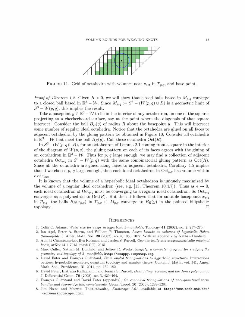
Proof. Apply Lemma 4.4, taking k sufficiently large so that ε(k) < ε. Then for any N > n(k),if p > N we obtain at least k consecutive ideal octahedra with volume as desired. Now letq > N , so q > k. Use the q–fold cover Mp,q → Mp,1. We obtain a k × q grid of octahedra,all of which have volume greater than (voct − ε(k)), as shown in Figure 11. �

We are now ready to complete the proof of Theorem 1.2.


Figure 11. Grid of octahedra with volumes near voct in Pp,q, and base point.

Proof of Theorem 1.2. Given R > 0, we will show that closed balls based in Mp,q convergeto a closed ball based in R3 −W. Since Mp,q := S3 − (W (p, q) ∪ B) is a geometric limit ofS3 −W (p, q), this implies the result.

Take a basepoint y ∈ R3−W to lie in the interior of any octahedron, on one of the squaresprojecting to a checkerboard surface, say at the point where the diagonals of that squareintersect. Consider the ball BR(y) of radius R about the basepoint y. This will intersectsome number of regular ideal octahedra. Notice that the octahedra are glued on all faces toadjacent octahedra, by the gluing pattern we obtained in Figure 10. Consider all octahedrain R3 −W that meet the ball BR(y). Call these octahedra Oct(R).

In S3−(W (p, q)∪B), for an octahedron of Lemma 2.1 coming from a square in the interiorof the diagram of W (p, q), the gluing pattern on each of its faces agrees with the gluing ofan octahedron in R3 −W. Thus for p, q large enough, we may find a collection of adjacentoctahedra Octp,q in S3 − W (p, q) with the same combinatorial gluing pattern as Oct(R).Since all the octahedra are glued along faces to adjacent octahedra, Corollary 4.5 impliesthat if we choose p, q large enough, then each ideal octahedron in Octp,q has volume withinε of voct.

It is known that the volume of a hyperbolic ideal octahedron is uniquely maximized bythe volume of a regular ideal octahedron (see, e.g. [13, Theorem 10.4.7]). Thus as ε → 0,each ideal octahedron of Octp,q must be converging to a regular ideal octahedron. So Octp,qconverges as a polyhedron to Oct(R). But then it follows that for suitable basepoints xp,qin Pp,q, the balls BR(xp,q) in Pp,q ⊂ Mp,q converge to BR(y) in the pointed bilipshcitztopology. �

References

1. Colin C. Adams, Waist size for cusps in hyperbolic 3-manifolds, Topology 41 (2002), no. 2, 257–270.2. Ian Agol, Peter A. Storm, and William P. Thurston, Lower bounds on volumes of hyperbolic Haken

3-manifolds, J. Amer. Math. Soc. 20 (2007), no. 4, 1053–1077, With an appendix by Nathan Dunfield.3. Abhijit Champanerkar, Ilya Kofman, and Jessica S. Purcell, Geometrically and diagrammatically maximal

knots, arXiv:1411.7915 [math.GT], 2015.4. Marc Culler, Nathan M. Dunfield, and Jeffrey R. Weeks, SnapPy, a computer program for studying the

geometry and topology of 3 -manifolds, http://snappy.computop.org.5. David Futer and Francois Gueritaud, From angled triangulations to hyperbolic structures, Interactions

between hyperbolic geometry, quantum topology and number theory, Contemp. Math., vol. 541, Amer.Math. Soc., Providence, RI, 2011, pp. 159–182.

6. David Futer, Efstratia Kalfagianni, and Jessica S. Purcell, Dehn filling, volume, and the Jones polynomial,J. Differential Geom. 78 (2008), no. 3, 429–464.

7. Francois Gueritaud and David Futer (appendix), On canonical triangulations of once-punctured torusbundles and two-bridge link complements, Geom. Topol. 10 (2006), 1239–1284.

8. Jim Hoste and Morwen Thistlethwaite, Knotscape 1.01, available at http://www.math.utk.edu/

∼morwen/knotscape.html.


9. Marc Lackenby, The volume of hyperbolic alternating link complements, Proc. London Math. Soc. (3) 88(2004), no. 1, 204–224, With an appendix by Ian Agol and Dylan Thurston.

10. Borut Levart, “Slicing a Torus” from the Wolfram Demonstrations Project,http://demonstrations.wolfram.com/SlicingATorus.

11. V. O. Manturov, A combinatorial representation of links by quasitoric braids, European J. Combin. 23(2002), no. 2, 207–212.

12. Skip Pennock, Turk’s-Head Knots (Braided Band Knots), A Mathematical Modeling, available athttp://www.mi.sanu.ac.rs/vismath/pennock1/index.html, 2005.

13. John G. Ratcliffe, Foundations of hyperbolic manifolds, Graduate Texts in Mathematics, vol. 149,Springer-Verlag, New York, 1994.

14. Igor Rivin, Euclidean structures on simplicial surfaces and hyperbolic volume, Ann. of Math. (2) 139(1994), no. 3, 553–580.

15. Morwen B. Thistlethwaite, A spanning tree expansion of the Jones polynomial, Topology 26 (1987), no. 3,297–309.

16. William P. Thurston, The geometry and topology of three-manifolds, Princeton Univ. Math. Dept. Notes,1979.

Department of Mathematics, College of Staten Island & The Graduate Center, City Uni-versity of New York, New York, NY

E-mail address: [email protected]

Department of Mathematics, College of Staten Island & The Graduate Center, City Uni-versity of New York, New York, NY

E-mail address: [email protected]

Department of Mathematics, Brigham Young University, Provo, UTE-mail address: [email protected]

Documents

VOLUME BOUNDS FOR WEAVING KNOTS Introductionjpurcell/papers/weaving.pdf · VOLUME BOUNDS FOR WEAVING KNOTS ABHIJIT CHAMPANERKAR, ILYA KOFMAN, AND JESSICA S. PURCELL Abstract. Weaving