Volume 10, Number 2, Pages 411–429 - ualberta.ca

INTERNATIONAL JOURNAL OF c© 2013 Institute for ScientificNUMERICAL ANALYSIS AND MODELING Computing and InformationVolume 10, Number 2, Pages 411–429

RESIDUAL-BASED A POSTERIORI ESTIMATORS FOR

THE T/Ω MAGNETODYNAMIC HARMONIC FORMULATION

OF THE MAXWELL SYSTEM

EMMANUEL CREUSE, SERGE NICAISE, ZUQI TANG, YVONNICK LE MENACH,

NICOLAS NEMITZ, AND FRANCIS PIRIOU

(Communicated by Mark Ainsworth)

Abstract. In this paper, we focus on an a posteriori residual-based error estimator for the T/Ωmagnetodynamic harmonic formulation of the Maxwell system. Similarly to the A/ϕ formulation[7], the weak continuous and discrete formulations are established, and the well-posedness ofboth of them is addressed. Some useful analytical tools are derived. Among them, an ad-hocHelmholtz decomposition for the T/Ω case is derived, which allows to pertinently split the error.Consequently, an a posteriori error estimator is obtained, which is proven to be reliable and locallyefficient. Finally, numerical tests confirm the theoretical results.

Key words. Maxwell equations, potential formulations, a posteriori estimators, finite elementmethod.

1. Introduction

Let us consider the electromagnetic fields, modeled by the well-known Maxwellsystem :

(1) curlE = −∂B∂t,

(2) curlH =∂D

∂t+ J,

where E is the electrical field, H the magnetic field, B the magnetic flux density,J the current flux density (or eddy current) and D the displacement flux densi-ty. Equation (1) is classically called Maxwell-Faraday equation and equation (2)Maxwell-Ampere one. In the low frequency regime, the quasistatic approximationcan be applied, which consists in neglecting the temporal variation of the displace-ment flux density with respect to the current density [12], such that the propagationphenomena are not taken into account. Consequently, equation (2) becomes :

(3) curlH = J.

Here, the current density J can be decomposed in two terms such that J = Js+Jec.Js is a known distribution current density generally generated by a coil, and Jec

represents the eddy current. Both equations (1) and (3) are linked by the materialconstitutive laws :

(4) B = µH,

(5) Jec = σE,

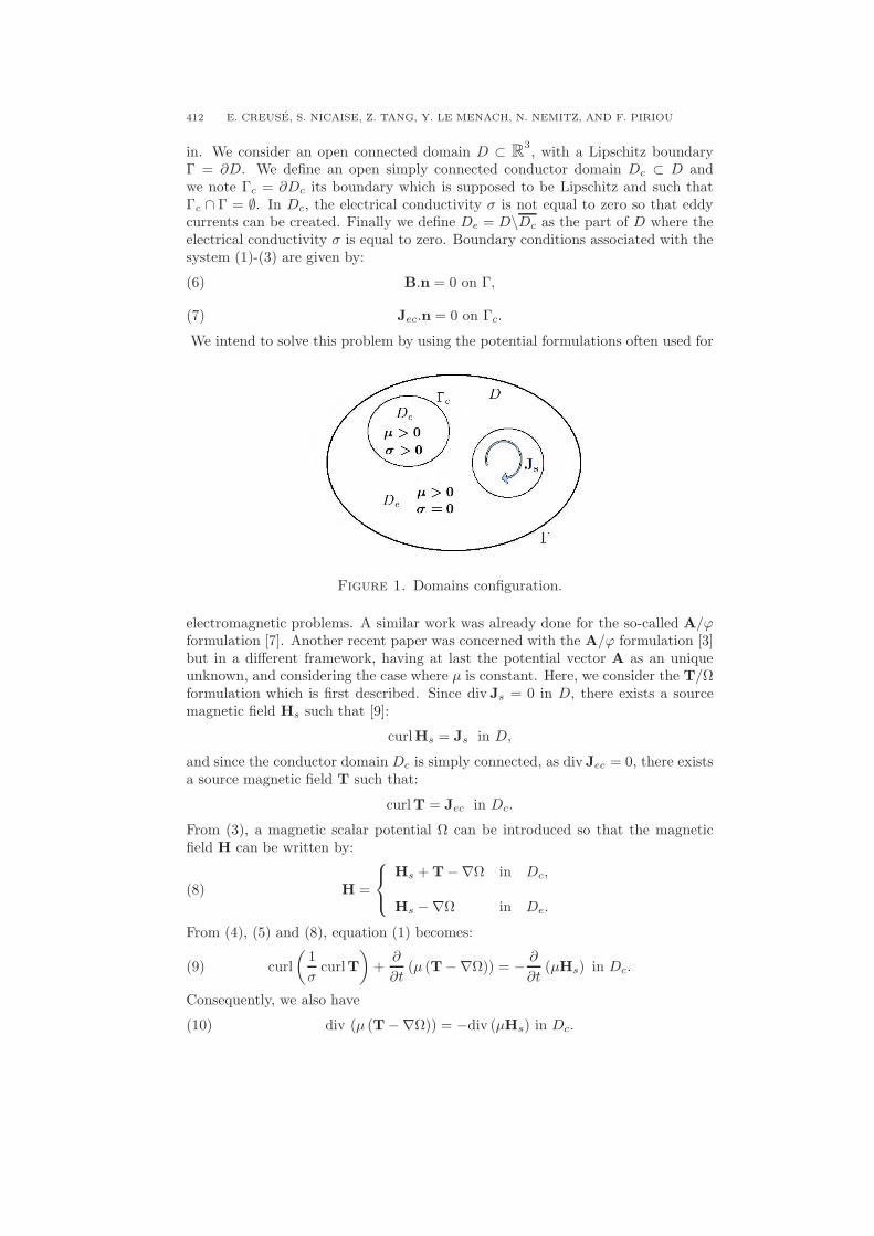
where µ stands for the magnetic permeability and σ for the electrical conductivityof the material. Figure 1 displays the domains configuration we are interested

Received by the editors and, in revised form, March 5, 2012.2000 Mathematics Subject Classification. 35Q61, 65N30, 65N15, 65N50.

411

412 E. CREUSE, S. NICAISE, Z. TANG, Y. LE MENACH, N. NEMITZ, AND F. PIRIOU

in. We consider an open connected domain D ⊂ R3, with a Lipschitz boundary

Γ = ∂D. We define an open simply connected conductor domain Dc ⊂ D andwe note Γc = ∂Dc its boundary which is supposed to be Lipschitz and such thatΓc ∩ Γ = ∅. In Dc, the electrical conductivity σ is not equal to zero so that eddycurrents can be created. Finally we define De = D\Dc as the part of D where theelectrical conductivity σ is equal to zero. Boundary conditions associated with thesystem (1)-(3) are given by:

(6) B.n = 0 on Γ,

(7) Jec.n = 0 on Γc.

We intend to solve this problem by using the potential formulations often used for

Figure 1. Domains configuration.

electromagnetic problems. A similar work was already done for the so-called A/ϕformulation [7]. Another recent paper was concerned with the A/ϕ formulation [3]but in a different framework, having at last the potential vector A as an uniqueunknown, and considering the case where µ is constant. Here, we consider the T/Ωformulation which is first described. Since div Js = 0 in D, there exists a sourcemagnetic field Hs such that [9]:

curlHs = Js in D,

and since the conductor domain Dc is simply connected, as div Jec = 0, there existsa source magnetic field T such that:

curlT = Jec in Dc.

From (3), a magnetic scalar potential Ω can be introduced so that the magneticfield H can be written by:

(8) H =

Hs +T−∇Ω in Dc,

Hs −∇Ω in De.

From (4), (5) and (8), equation (1) becomes:

(9) curl

(1

σcurlT

)+∂

∂t(µ (T−∇Ω)) = − ∂

∂t(µHs) in Dc.

Consequently, we also have

(10) div (µ (T−∇Ω)) = −div (µHs) in Dc.

A POSTERIORI ESTIMATORS FOR T − Ω FORMULATION 413

Moreover since divB = 0 in D, we get

(11) div (−µ∇Ω) = −div (µHs) in De.

The content of the paper is as follows. Section 2 establishes the weak formulationof the continuous and discrete problems, and the well-posedness of both of them isproven. In Section 3, we derive an ad-hoc Helmholtz decomposition of the error inthe conductor domain Dc. Section 3 is devoted to several analytical tools neededin the following of the paper. In Section 4, the reliability and the efficiency ofthe derived estimator are established. Finally, some numerical tests are treated inSection 5 to evaluate the estimator capabilities.

2. Weak formulation and discretization of the problem

2.1. Weak Formulation. From (9), (10) and (11), the T/Ω formulation of themagnetodynamic problem can be written:

(12)

curl

(1

σcurlT

)+∂

∂t(µ (T−∇Ω)) = − ∂

∂t(µHs) in Dc,

div (µ (T−∇Ω)) = −div (µHs) in Dc,

div (−µ∇Ω) = −div (µHs) in De.

We suppose that µ ∈ L∞(D) and that there exists µmin ∈ R∗+ such that µ > µmin

on D. We also assume that σ ∈ L∞(D), that there exists σmin ∈ R∗+ such that

σ > σmin on Dc, and we recall that σ|De≡ 0. Taking the associated boundary

conditions (6) and (7) into account, the harmonic formulation of the system (12)is given by: Find (T,Ω) ∈ V such that for all (T′,Ω′) ∈ V , we have

(13)

∫

Dc

1

σcurlT · curlT′ +

∫

Dc

jωµ (T−∇Ω) ·T′ =

∫

Dc

−jωµHs ·T′,

−∫

Dc

µ (T−∇Ω) · ∇Ω′ +

∫

De

µ∇Ω · ∇Ω′ =

∫

D

µHs · ∇Ω′,

where j2 = −1 and V = X0(Dc)× H1(D) with:

X(Dc) = H0(curl, Dc) =T ∈ L2(Dc); curlT ∈ L2(Dc) and T× n = 0 on Γc

,

X0(Dc) =

T ∈ X(Dc);

∫

Dc

T .∇ξ dx = 0, ∀ξ ∈ H10 (Dc)

,

H1(D) =

Ω ∈ H1(D);

∫

D

Ω = 0

.

In the following, on a given domain D, the L2(D) norm will be denoted by || · ||D,and the corresponding L2(D) inner product by (·, ·)D. The usual norm and semi-norm of H1(D) will be denoted by || · ||1,D and | · |1,D respectively. Now, X(Dc) isequipped with its usual norm :

‖T‖2X(Dc)= ‖T‖2L2(Dc)

+ ‖ curlT‖2L2(Dc),

and the natural norm ||.||V associated with the Hilbert space V is given by :

‖(T,Ω)‖2V = ||T||2X(Dc)+ |Ω|21,D.


It can be directly obtained that an equivalent variational formulation to (13) isgiven by : Find (T,Ω) ∈ V solution of

(14) a((T,Ω), (T′,Ω′)) = l((T′,Ω′)), ∀(T′,Ω′) ∈ V,

where a and l are respectively the following bilinear and linear forms defined by:

a((T,Ω), (T′,Ω′)) =

∫

Dc

1

σcurlT · curlT′ +

∫

Dc

jωµ(T−∇Ω) · (T′ −∇Ω′) +

∫

De

jωµ∇Ω · ∇Ω′,

l((T′,Ω′)) = −∫

Dc

jωµHs · (T′ −∇Ω′) +

∫

De

jωµHs · ∇Ω′.

2.2. Well-posedness of the problem.

Lemma 2.1. The bilinear form√2e−j π

4 a is coercive on V , namely there existsC > 0 such that:

∣∣√2e−j π4 a((T,Ω), (T,Ω))

∣∣ ≥ C∥∥(T,Ω)

∥∥2V.

Proof. First, let us notice that:

ℜ[√

2e−j π4 a ((T,Ω), (T,Ω))

]=

∫

Dc

1

σ

∣∣ curlT∣∣2+

∫

Dc

ωµ∣∣T−∇Ω

∣∣2+∫

De

ωµ∣∣∇Ω

∣∣2.

Our aim is to prove that there exists C > 0 such that for all (T,Ω) ∈ V ,∫

Dc

1

σ

∣∣ curlT∣∣2 +

∫

Dc

ωµ∣∣T−∇Ω

∣∣2 +∫

De

ωµ∣∣∇Ω

∣∣2 ≥ C∥∥(T,Ω)

∥∥2V.

This is done by an usual contradiction argument and using the fact that for T ∈X0(Dc), the Friedrichs-Poincare inequality ‖T‖L2(Dc) ≤ C‖ curlT‖L2(Dc) holds(see [11]). We refer to [7] for a similar proof in the A/ϕ formulation case.

Theorem 2.2. The weak formulation (14) admits a unique solution (T,Ω) ∈ V .

Proof. The sesquilinear form |√2e−j π

4 a| is obviously continuous on V × V andcoercive on V by Lemma 2.1. So Lax-Milgram’s lemma ensures existence anduniqueness of a solution (T′,Ω′) ∈ V to (14).

Lemma 2.3. Let (T′,Ω′) ∈ V be the unique solution of (14). Then for all(T′,Ω′) ∈ X(Dc)×H1(D), we have :

a ((T,Ω), (T′,Ω′)) = l ((T′,Ω′)) .

Proof. Since T′ ∈ X(Dc), we can decompose it using the following Helmholtzdecomposition [11, p. 66]:

T′ = Ψ+∇τ,where Ψ ∈ X0(Dc) and τ ∈ H1

0 (Dc). It is known that for any function Ω′ ∈ H1(D),

we can find Ω′ ∈ H1(D) such that ∇Ω′ = ∇Ω′ by the definition:

Ω′ = Ω′ − 1

|D|

∫

D

Ω′.


We write

a((T,Ω), (T′,Ω′)) = a((T,Ω), (Ψ +∇τ,Ω′))

=

∫

Dc

1

σcurlT · curlΨ +

∫

Dc

jωµ(T−∇Ω) · (Ψ −∇(Ω′ − τ)) +

∫

De

jωµ∇Ω · ∇Ω′

=

∫

Dc

1

σcurlT · curlΨ +

∫

Dc

jωµ(T−∇Ω) · (Ψ −∇Ω′) +

∫

De

jωµ∇Ω · ∇Ω′,

where we define Ω′ ∈ H1(D) by

Ω′ =

Ω′ − τ +1

|D|

∫

Dc

τ in Dc,

Ω′ +1

|D|

∫

Dc

τ in De.

Therefore we conclude that:

(15) a((T,Ω), (Ψ +∇τ,Ω′)) = a((T,Ω), (Ψ, Ω′)).

Similarly it is clear that

l((T′,Ω′)) = l((Ψ +∇τ,Ω′))

= −∫

Dc

jωµHs · (Ψ −∇Ω′) +

∫

De

jωµHs · ∇Ω′

= l((Ψ, Ω′)).

Taking into account that Ψ ∈ X0(Dc) and Ω′ ∈ H1(D), from (14), we get

(16) a((T,Ω), (Ψ, Ω′)) = l((Ψ, Ω′)).

From (15) and (16) we conclude that

a((T,Ω), (T′,Ω′)) = l((T′,Ω′)).

2.2.1. Discrete formulation. Now, the boundaries Γc and Γ are supposed to bepolyhedral such that the domain D can be discretized by a conforming mesh Th

made of tetrahedra, each element T of Th belonging either to Dc or De. The facesof Th are denoted by F and its edges by E. Let us denote by hT the diameterof T and ρT the diameter of its largest inscribed ball. We suppose that for anyelement T , the ratio hT /ρT is bounded by a constant α > 0 independant of T andof the mesh size h = max

T∈Th

hT . The set of faces (resp. edges and nodes) of the

triangulation is denoted F (resp. E and N ), and we denote hF the diameter of theface F . The set of internal faces (resp. internal edges and internal nodes) to D isdenoted Fint (resp. Eint and Nint). The coefficients µ and σ arising in (12) aremoreover supposed to be constant on each tetrahedron of the mesh, and we willnote µT = µ|T and σT = σ|T for all T ∈ Th.

The approximation space Vh is defined by Vh = X0h × Θh, where :

Xh(Dc) = X(Dc) ∩ ND1(Dc,Th) =Th ∈ X(Dc);Th|T ∈ ND1(T ), ∀ T ∈ Th

,


ND1(T ) =

Th :

T −→ C3

x −→ a+ b× x, a,b ∈ C

3

,

Θh =Ωh ∈ H1(D); Ωh|T ∈ P1(T ) ∀ T ∈ Th

,

Θ0h =

ξh ∈ H1

0 (Dc); ξh|T ∈ P1(T ) ∀ T ∈ Th

,

X0h(Dc) =

Th ∈ Xh(Dc); (Th,∇ξh)Dc = 0 ∀ ξh ∈ Θ0

h

,

Θh =Ωh ∈ H1(D); Ωh|T ∈ P1(T ) ∀ T ∈ Th

.

Now, the discretized weak formulation associated with (14) consists in finding(Th,Ωh) ∈ Vh such that for all (T′

h,Ω′h) ∈ Vh, we have :

(17) a((Th,Ωh), (T′h,Ω

′h)) = l((T′

h,Ω′h)).

Theorem 2.4. The weak formulation (17) admits a unique solution (Th,Ωh) ∈ Vh.

Proof. The proof is in any point similar to the one of Theorem 2.2 for the continuouscase. The main point relies in proving the coercivity of a on Vh, which can be doneby using the discrete Poincare-Friedrichs inequality ||Th|| ≤ C|| curlTh|| for allTh ∈ X0

h(Dc), with C > 0 independent of h, see [11, p. 185].

Remark 2.5. Let us notice that, because of the discrete Gauge condition arisingin the definition of X0

h, Vh is not included in V , so that the approximation is not aconforming one.

Lemma 2.6. For all (T′h,Ω

′h) ∈ Xh(Dc)×Θh, we have:

a((Th,Ωh), (T′h,Ω

′h)) = l((T′

h,Ω′h)).

Proof. : Since T′h ∈ Xh(Dc), this time we can use the discrete Helmholtz decom-

position [8, p. 272]:

T′h = Ψh +∇τh with Ψh ∈ X0

h(Dc) and τh ∈ Θ0h.

The proof is then very similar to the one for the continuous case, see Lemma 2.3.

A direct consequence of Lemmas 2.3 and 2.6 is the following orthogonality prop-erty, despite the fact that the approximation is not a conforming one :

Lemma 2.7. For all (T′h,Ω

′h) ∈ Xh(Dc)×Θh

a((T−Th,Ω− Ωh), (T′h,Ω

′h)) = 0.

3. Helmholtz decomposition

In the following, the notations a . b and a ∼ b mean the existence of positiveconstants C1 and C2 which are independent of the quantities a and b under consid-eration as well as of the mesh size h, the coefficients µ, σ and of the frequency ω,such that a ≤ C2b and C1b ≤ a ≤ C2b, respectively.


Helmholtz decomposition. Compared to the work on the A/ϕ formulation [7],one suitable Helmholtz decomposition has to be found for the T/Ω formulation.Let us define the errors on T and Ω by:

(18) eT = T−Th ∈ H0(curl, Dc),

(19) eΩ = Ω− Ωh ∈ H1(D).

Let XN (Dc) denote the space:

XN (Dc) = u ∈ H(curl, Dc) ∩H(div , Dc),u× n = 0 on Γcequipped with the norm:

∥∥u∥∥2XN (Dc)

=∥∥u∥∥2L2(Dc)

+∥∥divu

∥∥2L2(Dc)

+∥∥ curlu

∥∥2L2(Dc)

.

Theorem 3.1. The error eT −∇eΩ admits the following Helmholtz decompositionin the conductor domain Dc:

eT −∇eΩ = Ψ+∇Φ +∇(ψ − eΩ),

where Ψ ∈ H1(Dc) ∩XN (Dc), Φ ∈ H10 (Dc) and ψ ∈ H1

0 (Dc), with∥∥Ψ∥∥2H1(Dc)

+∥∥∇Φ

∥∥2L2(Dc)

+∥∥∇(ψ − eΩ)

∥∥2L2(Dc)

.∥∥eT −∇eΩ

∥∥2L2(Dc)

+∥∥∇eΩ

∥∥2L2(De)

+∥∥ curl eT

∥∥2L2(Dc)

.

Proof. Let us define

(20) eΩ = eΩ − 1

|De|

∫

De

eΩ.

Since eΩ ∈ H1(D), we have eΩ ∈ H1(Dc) and eΩ ∈ H1(De), which leads to

eΩ ∈ H1(Dc) and eΩ ∈ H1(De).First of all, let us define ψ ∈ H1

0 (Dc) such that

div∇ψ = div eT in Dc,ψ = 0 on Γc.

The definition w = eT −∇ψ yields

(21) curlw = curleT in Dc.

Clearly, w ∈ XN(Dc). From (20) we get

eT −∇eΩ = eT −∇eΩ

= w+∇(ψ − eΩ).

From [1] we know that the embedding of XN (Dc) into L2(Dc)

3 is compact, so that∥∥w∥∥2XN (Dc)

.∥∥divw

∥∥2L2(Dc)

+∥∥ curlw

∥∥2L2(Dc)

.

Since divw = 0, we have

(22)∥∥w∥∥2XN (Dc)

.∥∥ curlw

∥∥2L2(Dc)

.

By (21), we can conclude that:

(23)∥∥w∥∥2L2(Dc)

≤∥∥w∥∥2XN (Dc)

.∥∥ curleT

∥∥2L2(Dc)

,


and(24)∥∥eT −∇eΩ

∥∥2L2(Dc)

=

∫

Dc

(w+∇ψ −∇eΩ) · (w+∇ψ −∇eΩ)

=

∫

Dc

|w|2 +∫

Dc

|∇(ψ − eΩ)|2 + 2

∫

Dc

w · ∇(ψ − eΩ).

Using Green’s formula∫

Dc

w · ∇(ψ − eΩ) =

∫

Γc

w · n · (ψ − eΩ)−∫

Dc

divw · (ψ − eΩ)

= −∫

Γc

w · n · eΩ since divw = 0 and ψ|Γc = 0

.∥∥w · n

∥∥H−1/2(Γc)

·∥∥eΩ

∥∥H1/2(Γc)

.

Applying the trace theorem, we have:∥∥eΩ

∥∥H1/2(Γc)

.∥∥eΩ

∥∥H1(De)

,

and Theorem 2.5 in [8, p. 27] leads to:∥∥w · n

∥∥H−1/2(Γc)

. ‖w‖H(div,Dc) = ‖w‖L2(Dc) .

From (23), we get∥∥w · n

∥∥H−1/2(Γc)

.∥∥ curl eT

∥∥L2(Dc)

,

so that ∫

Dc

w · ∇(ψ − eΩ) .∥∥ curl eT

∥∥2L2(Dc)

+∥∥eΩ

∥∥2H1(De)

.

Taking into account (24), we get:∥∥w∥∥2L2(Dc)

+∥∥∇(ψ−eΩ)

∥∥2L2(Dc)

.∥∥eT−∇eΩ

∥∥2L2(Dc)

+∥∥eΩ

∥∥2H1(De)

+∥∥ curleT

∥∥2L2(Dc)

.

Since eΩ ∈ H1(De), Poincare’s inequality∥∥eΩ

∥∥2H1(De)

.∥∥∇eΩ

∥∥2L2(De)

holds. Hence

we have:(25)∥∥w∥∥2L2(Dc)

+∥∥∇(ψ−eΩ)

∥∥2L2(Dc)

.∥∥eT−∇eΩ

∥∥2L2(Dc)

+∥∥∇eΩ

∥∥2L2(De)

+∥∥ curleT

∥∥2L2(Dc)

.

Finally from [5], we get

XN (Dc) = XN(Dc) ∩H1(Dc)3 +∇H1

0 (Dc),

which implies that

w = Ψ+∇Φ,

where Ψ ∈ H1(Dc)3 ∩XN (Dc) and Φ ∈ H1

0 (Dc), with:

(26)∥∥Ψ∥∥H1(Dc)

+∥∥∇Φ

∥∥L2(Dc)

.∥∥w∥∥XN (Dc)

.

(25), (26) associated with (21) and (22) conclude the proof.

Applying a change with variables, we can have the following corollary:


Corollary 3.2. The error eT −∇eΩ admits the following decomposition in Dc:

eT −∇eΩ = Ψ+∇Φ +∇eΩ,where Ψ ∈ H1(Dc) ∩XN (Dc), Φ ∈ H1

0 (D) and eΩ ∈ H1(D). Moreover,∥∥Ψ∥∥2H1(Dc)

+∥∥∇Φ

∥∥2L2(D)

+∥∥∇eΩ

∥∥2L2(D)

.∥∥eT−∇eΩ

∥∥2L2(Dc)

+∥∥∇eΩ

∥∥2L2(De)

+∥∥ curl eT

∥∥2L2(Dc)

.

Proof. Using the notation of Theorem 3.1, let us define Φ by:

(27) Φ =

Φ in Dc,0 in De.

Since Φ ∈ H10 (Dc), we have that Φ ∈ H1

0 (D) and ‖∇Φ‖L2(D) = ‖∇Φ‖L2(Dc).Let us also define eΩ by:

(28) eΩ =

ψ − eΩ in Dc,−eΩ in De.

Since ψ ∈ H10 (Dc) and eΩ ∈ H1(D), clearly eΩ ∈ H1(D) and∥∥∇eΩ

∥∥2L2(D)

=∥∥∇(ψ − eΩ)

∥∥2L2(Dc)

+∥∥∇eΩ

∥∥2L2(De)

.

4. Analytical tools

For completeness, this section defines and recalls some usual analytical tools usedin the following of the paper to make it self-contained.

4.1. Standard Clement interpolation operator. For our further analysis, weneed an interpolation operator that maps a function from H1

0 (D) to Θ0h(D) =

ξh ∈ H1(D); ξh|T ∈ P1(T ) ∀ T ∈ Th ∩D, as well as an interpolation operator

that maps a function from H1(D) to Θh. Hence Lagrange interpolation is un-suitable, but Clement like interpolant is more appropriate. Recall that the nodalbasis functions ϕx ∈ Θ0

h associated with a node x is uniquely determined by thecondition :

ϕx(y) = δx,y, ∀y ∈ N .

Moreover, for any x ∈ N , we define Dx as the set of tetrahedra containing the nodex.

Definition 4.1. We define the Clement interpolation operator I0Cl : H10 (D) →

Θ0h(D) by :

I0Clv =∑

x∈Nint

1

|Dx|( ∫

Dx

v)ϕx,

where Dx is the set of tetrahedra containing the node x.

Definition 4.2. We define the Clement interpolation operator ICl : H1(D) → Θh

by :

IClv =∑

x∈N∩D

1

|Dx ∩D|( ∫

Dx∩D

v)ϕx,

Then, we can state the following usual interpolation estimates :


Lemma 4.3. For any v0 ∈ H10 (D) and v ∈ H1(D) it holds :

∑

T∈Th

h−2T ||v0 − I0Clv

0||2T . ||∇v0||2L2(D),(29)

∑

F∈Fint

h−1F ||v0 − I0Clv

0||2F . ||∇v0||2L2(D),(30)

∑

T∈Th,T⊂D

h−2T ||v − IClv||2T . ||∇v||2L2(D),(31)

∑

F∈F ,F⊂D

h−1F ||v − IClv||2F . ||∇v||2L2(D).(32)

Proof. See [4].

4.2. Vectorial Clement-type interpolation operator. Since our problem alsoinvolves functions in X(Dc), we further need a Clement-type interpolant mappinga (vector) function in X(Dc) to Xh(Dc). This operator was introduced in [6] in ananisotropic context (for an isotropic version, see [2]), we recall it here. It is definedwith the help of the basis functions wE ∈ Xh, E ∈ E , defined by the condition :

∫

E′

wE .TE′ = δE,E’, ∀E′ ∈ E ,

where TE means the unit vector directed along E. Let us define PH1(Dc) as theset of functions which are piecewise H1 on the domain Dc, as well as ∇P the socalled ”broken gradient” associated with this decomposition.

Definition 4.4. For any edge E ∈ E fix one of its adjacent faces that we callFE ∈ F . Then define the Clement type interpolation operator PCl : [PH

1(Dc)] ∩X(Dc) → Xh(Dc) by :

PClv =∑

E∈E

( ∫

FE

(v× nFE ) · fFE

E

)wE ,

where the (vector) functions fFE

E′ are determined by the condition :∫

FE

(wE′ × nFE ) · fFE

E′′ = δE′,E′′ , ∀E′, E′′ ∈ E ∪ ∂FE .

Then, we can state the following usual interpolation estimates :

Lemma 4.5. For all v ∈ [PH1(Dc)] ∩X(Dc), we have :∑

T∈Th

h−2T ||v− PClv||2T . ||∇P v||2,(33)

∑

F∈F

h−1F ||v− PClv||2F . ||∇P v||2.(34)

Proof. See [2].

5. A posteriori error estimation

5.1. Definition of the residual. For all (T′,Ω′) ∈ X(Dc)×H1(D), the residualis defined by :

(35) r((T′,Ω′)) = l((T′,Ω′))− a((Th,Ωh), (T′,Ω′))


Lemma 5.1. Let us recall that eT and eΩ are respectively defined by (18) and (19).Then we have:(36)

ℜ[√

2e−j π4 r ((eT, eΩ))

]=

∫

Dc

1

σ

∣∣ curl eT∣∣2 +

∫

Dc

ωµ∣∣eT −∇eΩ

∣∣2 +∫

De

ωµ∣∣∇eΩ

∣∣2

Now, we are interested in deriving an a posteriori error estimator in order to con-trol the error defined as the right-hand-side of (36). Consequently, we are reduced

to bound from above the quantity∣∣∣r ((eT, eΩ))

∣∣∣.

5.2. Definition of the estimators. Let us consider T a given tetrahadron of thetriangulation. Hh is defined on T by:

Hh =

Hs +Th −∇Ωh if T ⊂ Dc,

Hs −∇Ωh if T ⊂ De.

Let F be a common face of the tetrahedra T1 and T2, we define the normal jumpof the quantity v through the face F by:

[v · n

]F= vT1

· nT1+ vT2

· nT2

and the tangential jump of the quantity v through the face F by:[v× n

]F= vT1

× nT1+ vT2

× nT2,

where, nTi stands for the outward unit normal of Ti on F (i=1,2). In the casewhere F is on the boundary Γ, we set: vT2

= 0.In the case where F is on the internal boundary Γc, T1 ⊂ Dc and T2 ⊂ De, as

Th does not exist in De, we define:[n× 1

σcurlTh

]F= nT1

× 1

σT1

curlThT1.

Definition 5.2. The local error estimator on the tetrahedron T is defined by:

• 1st case: T ⊂ Dc

η2T = η2T ;1 + η2T ;2 +∑

F⊂∂T

(η2F ;1 + η2F ;2),

• 2nd case: T ⊂ De

η2T = η2T ;2 +∑

F⊂∂T

η2F ;2,

with

ηT ;1 = hT

∥∥∥∥− curl(1

σcurlTh)− jωµHh

∥∥∥∥T

,

ηT ;2 = hT∥∥div (jωµHh)

∥∥T= 0,

ηF ;1 = h1/2F

∥∥∥∥[n× 1

σcurlTh

]F

∥∥∥∥F

,

ηF ;2 = h1/2F ω

∥∥∥[n · µHh

]F

∥∥∥F.


Moreover, the global error estimator is defined by:

η2 =∑

T∈T

η2T .

Remark 5.3. Despite the fact that ηT ;2 = 0 because of the low order finite elementspaces used here, we let them for the sake of completeness, having in mind thattheir contributions have to be taken into account for higher degree discretizations.

5.3. Reliability.

Theorem 5.4. We have :(∫

Dc

1

σ

∣∣ curl eT∣∣2 +

∫

Dc


∣∣2 +∫

De

ωµ∣∣∇eΩ

∣∣2)1/2

. Cup η,

with

Cup = max

1

ω1/2 minT∈D

µ1/2T

, maxT∈Dc

σ1/2T

.

Proof. Proof is similar to the ones given in the A/ϕ formulation [7], but with thenew Helmholtz decomposition given in section 3.

By (35), we have

r((eT, eΩ)) = l((eT, eΩ))− a((Th,Ωh), (eT, eΩ))

= −∫

Dc

jωµHs · (eT −∇eΩ) +∫

De

jωµHs · ∇eΩ

−∫

Dc

1

σcurlTh · curl eT −

∫

Dc

jωµ(Th −∇Ωh) · (eT −∇eΩ)

−∫

De

jωµ∇Ωh · ∇eΩ.

Taking into account (20) and the fact that curl∇eΩ = 0, we have

r((eT, eΩ)) = −∫

Dc

jωµHs · (eT −∇eΩ) +∫

De

jωµHs · ∇eΩ

−∫

Dc

1

σcurlTh · curl(eT −∇eΩ)

−∫

Dc

jωµ(Th −∇Ωh) · (eT −∇eΩ)

−∫

De

jωµ∇Ωh · ∇eΩ

Applying the Helmholtz decomposition in Corollary 3.2,

eT −∇eΩ = Ψ+∇Φ+∇(ψ − eΩ),

we get

r((eT, eΩ)) = −∫

Dc

jωµHs · (Ψ +∇Φ +∇(ψ − eΩ))

+

∫

De

jωµHs · ∇eΩ −∫

Dc

1

σcurlTh · curlΨ

−∫

Dc

jωµ(Th −∇Ωh) · (Ψ +∇Φ +∇(ψ − eΩ))

−∫

De

jωµ∇Ωh · ∇eΩ


From (27) and (28), we get:

|r((eT, eΩ))| =

∣∣∣∣−∫

Dc

jωµHs ·Ψ−∫

D

jωµHs · ∇Φ −∫

D

jωµHs · ∇eΩ

−∫

Dc

1

σcurlTh · curlΨ−

∫

Dc

jωµ(Th −∇Ωh) ·Ψ

−∫

Dc

jωµ(Th −∇Ωh) · ∇Φ−∫

Dc

jωµ(Th −∇Ωh) · ∇eΩ

+

∫

De

jωµ∇Ωh · ∇eΩ +

∫

De

jωµ∇Ωh · ∇Φ

∣∣∣∣

Introducing the three Clement interpolation operators PCl, ICl and I0Cl, the or-thogonality property from lemma 2.7 leads to:

|r((eT, eΩ))| =

∣∣∣∣−∫

Dc

jωµHs ·Ψ− PCl Ψ−∫

D

jωµHs · ∇(Φ− I0Cl Φ)

−∫

D

jωµHs · ∇(eΩ − ICl eΩ)−∫

Dc

1

σcurlTh · curl(Ψ − PCl Ψ)

−∫

Dc

jωµ(Th −∇Ωh) ·Ψ− PCl Ψ

−∫

Dc

jωµ(Th −∇Ωh) · ∇(Φ− I0Cl Φ)

−∫

Dc

jωµ(Th −∇Ωh) · ∇(eΩ − ICl eΩ)

+

∫

De

jωµ∇Ωh · ∇(eΩ − ICl eΩ) +

∫

De

jωµ∇Ωh · ∇(Φ− I0Cl Φ)

∣∣∣∣

Using Green’s formula on each tetrahedron and the continuous as well as discreteCauchy-Schwarz inequality, we obtain:

|r((eT, eΩ))|

.

( ∑

T∈Th∩Dc

η2T ;1

)1/2( ∑

T∈Th∩Dc

h−2T ‖Ψ− PCl Ψ‖2T

)1/2

+

( ∑

T∈Th

η2T ;2

)1/2( ∑

T∈Th

h−2T

∥∥∥Φ− I0Cl Φ∥∥∥2

T

)1/2

+

( ∑

T∈Th

η2T ;2

)1/2( ∑

T∈Th

h−2T ‖eΩ − ICl eΩ‖2F

)1/2

+

( ∑

F∈F∩Dc

η2F ;1

)1/2( ∑

F∈F∩Dc

h−1F ‖Ψ− PCl Ψ‖2F

)1/2

+

(∑

F∈F

η2F ;2

)1/2(∑

F∈F

h−1F

∥∥∥Φ− I0Cl Φ∥∥∥2

F

)1/2

+

(∑

F∈F

η2F ;2

)1/2(∑

F∈F

h−1F ‖eΩ − ICl eΩ‖2F

)1/2

Now, we deduce from inequalities (29) to (34) that :


|r((eT, eΩ))|

.

( ∑

T∈Th∩Dc

η2T ;1

)1/2 ∥∥Ψ∥∥H1(Dc)

+

( ∑

T∈Th

η2T ;2

)1/2 ∥∥∇Φ∥∥L2(D)

+

( ∑

T∈Th

η2T ;2

)1/2 ∥∥∇eΩ∥∥L2(D)

+

( ∑

F∈F∩Dc

η2F ;1

)1/2 ∥∥Ψ∥∥H1(Dc)

+

(∑

F∈F

η2F ;2

)1/2 ∥∥∇Φ∥∥L2(D)

+

(∑

F∈F

η2F ;2

)1/2 ∥∥∇eΩ∥∥L2(D)

Theorem 3.2 yields:∥∥Ψ∥∥2H1(Dc)

+∥∥∇Φ

∥∥2L2(D)

+∥∥∇eΩ

∥∥2L2(D)

.∥∥eT −∇eΩ

∥∥2L2(Dc)

+∥∥∇eΩ

∥∥2L2(De)

+∥∥ curl eT

∥∥2L2(Dc)

.∥∥ω

1/2µ1/2

ω1/2µ1/2(eT −∇eΩ)

∥∥2L2(Dc)

+∥∥ω

1/2µ1/2

ω1/2µ1/2∇eΩ

∥∥2L2(De)

+∥∥σ

1/2

σ1/2curl eT

∥∥2L2(Dc)

.1

ω minT∈Dc

µT

∥∥ω1/2µ1/2(eT −∇eΩ)∥∥2L2(Dc)

+1

ω minT∈De

µT

∥∥ω1/2µ1/2∇eΩ∥∥2L2(De)

+ maxT∈Dc

σT∥∥ 1

σ1/2curleT

∥∥2L2(Dc)

. Cup

(∫

Dc

1

σ

∣∣ curleT∣∣2 +

∫

Dc


∣∣2 +∫

De

ωµ∣∣∇eΩ

∣∣2)1/2

where Cup = max

1

ω1/2 minT∈D

µ1/2T

, maxT∈Dc

σ1/2T

.

5.4. Efficiency. Now, in order to derive the efficiency of our estimator, we have tobound each part of the estimator by the local error. Reiterating, proofs are basedon the same kind of arguments than the ones given in A/ϕ formulation [7]. Due tothis reason, these proofs can not be recalled here.

Theorem 5.5. Let us define PT =⋃

T ′∩T 6=∅

T ′, we have the efficiency of our esti-

mator:

ηT . CT,down(∥∥∥σ−1/2 curl eT

∥∥∥2

PT

+∥∥∥ω1/2µ1/2(eT −∇eΩ)

∥∥∥2

PT

+∥∥∥ω1/2µ1/2∇eΩ

∥∥∥2

PT

)1/2 + h.o.t,

with

CT,down = maxT ′∈PT

ω1/2µ

1/2T ′ ,

1

σ1/2T ′

.

Proof. We have to bound each part of the estimator by a local error which is donewith the so-called bubble functions and inverse inequalities. We refer to [7] for thedetails about the A/ϕ formulation.

6. Numerical validation

In this section, a physical test is considered [10]. The computation model consistsof a coil between two symmetrical conductors shown in Figure 2 for five differentrefined meshes. Here, we set µ = 4π 10−7 H/m and σ = 3.28 107Ω/m in the


conductors. When a current is imposed in the coil, the eddy current Jec = curlTis generated in the two conductor plates.

(a) Mesh 1 (b) Mesh 2 (c) Mesh 3

(d) Mesh 4 (e) Mesh 5

Figure 2. Domain and Mesh of the Problem.

To begin with, the value of the estimator η is displayed as a function of themaximum diameter of the tetrahedra h corresponding to each mesh (see Figure 3).It shows a good behavior of the estimator compared with the theoretically expectedresults since it converges well towards zero.

−1.5 −1.4 −1.3 −1.2 −1.1 −1 −0.9 −0.8 −0.7 −0.6−1

−0.5

0

0.5

Log(h)

Log(

Est

imat

or)

Log(Estimator)

Figure 3. Estimator versus h.

Now, in Figure 4 a unique given mesh in chosen to perform the following tests.Let us note that the part of the mesh in the upper conductor is finer that the partof the mesh in the lower one.


Figure 4. Domain and Mesh of the Problem.

As shown in Figure 5(a) and 5(b), the real and the imaginary parts of theeddy current vector field at the frequency of 50 Hz lies in the down surface of theupper conductor plate. The eddy current resembles the physically expected onequalitatively.

(a) Real part. (b) Imaginary part.

Figure 5. Top view of the eddy current at 50 Hz in the downsurface of the upper conductor plate.

As numerically expected, the error in the lower plate is larger than the one above,as shown by the local estimators ηT maps in Figure 6(a) and 6(b).

At the end of this section, we want to underline the skin-effect phenomenon onthe above conductor plate. In normal cases, the skin depth δ is well approximatedas [15, p.504]:

δ =

√2

ωµσ.

As shown in Figure 7(a), 7(b) and 7(c), the estimator allows to detect the areasof the domain where the mesh needs to be refined in order to track this skin-effectphenomenon.


0.000211491

0.000158642

0.000105794

5.29450e-05

9.62847e-08

ESTIMATEUR_DYNAMIQUE_REAL 0, -

(a) Upper plate

0.0176072

0.0132195

0.00883188

0.00444423

5.65668e-05


(b) Lower plate

Figure 6. Local estimator ηT maps in the two conductor platesat frequency 50 Hz.

0.000211491

0.000158642

0.000105794

5.29450e-05

9.62847e-08


(a) 50 Hz.

0.00369202

0.00276904

0.00184605

0.000923065

8.03685e-08


(b) 500 Hz.

0.0656678

0.0492509

0.0328340

0.0164171

1.90604e-07


(c) 5000 Hz.

Figure 7. Local estimator ηT maps in the upper conductor plate.


Possible extension

The referee of this paper suggested to treat the case where Dc is no more simplyconnected, for which the variational formulation (14) is no more valid. For example,in the case where Dc is a torus, the weak formulation of the problem is stated in[13]. Unfortunately, we did not succeed in deriving the estimator in that case,because Theorem 3.1 is no more applicable.

References

[1] C. Amrouche, C. Bernardi, M. Dauge and V. Girault, Vector Potentials in Three-dimensionalNon-smooth Domains, Math. Meth. in the Applied Sciences 21 (1998), 823-864.

[2] R. Beck, R. Hiptmair, R. H. W. Hoppe, B. Wohlmuth, Residual based a posteriori errorestimators for eddy current computation, M2AN Math. Model. Numer. Anal., 34 (2000),159-182.

[3] J. Chen, Z. Chen, T. Cui, L. Zhang, An adaptive finite element method for the eddy currentmodel with circuit/field couplings, SIAM J. Sci. Comput. 32 (2010), no. 2, 1020-1042.

[4] P. Clement, Approximation by finite element functions using local regularization. Rev.Francaise. Automat. Informat. Recherche Operationnelle Ser. R.A.I.R.O. Anal. Numr.9(R2):77-84, 1975.

[5] M. Costabel, M. Dauge and S. Nicaise, Singularities of Maxwell Interface Problems, ModelMath. Anal. Numer. 33 (1999) 627-649.

[6] E. Creuse and S. Nicaise, Anisotropic a posteriori error estimation for the mixed discontinuousGalerkin approximation of the Stokes problem, Numerical Methods in Partial DifferentialEquations, vol. 22, no 2, 449-483, 2006.

[7] E. Creuse, S. Nicaise, Z. Tang, Y. Le Menach, N. Nemitz, F. Piriou, Residual-based a poste-riori estimators for the A/ϕ magnetodynamic harmonic formulation of the Maxwell system,Mathematical Models and Methods in Applied Sciences, to appear.

[8] V. Girault and P.A. Raviart, Finite element methods for Navier-Stokes equations, volume 5of Springer Series in Computational Mathematics. Springer-Verlag, Berlin, 1986. Theory andalgorithms.

[9] Y. Le Menach, S. Clenet, and F. Piriou, Determination and utilization of source field in 3-Dmagnetostatic problem, IEEE Trans. Magn., vol. 34, pp.2509 - 2511 , 1998.

[10] P. J. Leonard and D. Rodger, Voltage forced coils for 3-D finite element method electromag-netic model, IEEE Trans. Magn., vol. 24, 2579 - 2581, 1988.

[11] P. Monk, Finite element methods for Maxwell’s equations. Numerical Mathematics and Sci-entific Computation. Oxford University Press, New York, 2003.

[12] A.A. Rodriguez, R. Hiptmair, and A. Valli, Hybrid formulations of eddy current problems.Numer. Method. Part. Differ. Eq., 21(4):742-763, 2005.

[13] A.A. Rodrıguez and A. Valli, Eddy current approximation of Maxwell equations, MS&A.Modeling, Simulation and Applications, vol. 4, Theory, algorithms and applications, Springer-Verlag Italia, Milan, 2010.

[14] R. Verfurth, A review of a posteriori error estimation and adaptive mesh-refinement tech-niques. Chichester and Stuttgart: Wiley and Teubner, Amsterdam, 1996.

[15] J. A. Stratton, Electromagnetic Theory, McGraw - Hill (1941).


LPP UMR 8524 and INRIA Lille Nord Europe, Universite de Lille 1, Cite Scientifique, 59655Villeneuve d’Ascq Cedex, France.

E-mail : [email protected]: http://math.univ-lille1.fr/∼creuse/

LAMAV, FR CNRS 2956, Universite de Valenciennes et du Hainaut Cambresis, Institut des

Sciences et Techniques de Valenciennes, F-59313 - Valenciennes Cedex 9, France.E-mail : [email protected]

L2EP, Universite de Lille 1, Cite Scientifique, 59655 Villeneuve d’Ascq Cedex,France.E-mail : [email protected]

L2EP, Universite de Lille 1, Cite Scientifique, 59655 Villeneuve d’Ascq Cedex, France.E-mail : [email protected]

THEMIS, EDF R&D, 1 avenue du General de Gaulle, BP408, 92141 Clamart Cedex.E-mail : [email protected]

L2EP, Universite de Lille 1, Cite Scientifique, 59655 Villeneuve d’Ascq Cedex, France.E-mail : [email protected]

Documents

Volume 10, Number 2, Pages 411–429 - ualberta.ca