Embed Size (px)
Citation preview

HAL Id: hal-00768974https://hal.archives-ouvertes.fr/hal-00768974
Submitted on 20 Oct 2015
HAL is a multi-disciplinary open accessarchive for the deposit and dissemination of sci-entific research documents, whether they are pub-lished or not. The documents may come fromteaching and research institutions in France orabroad, or from public or private research centers.
L’archive ouverte pluridisciplinaire HAL, estdestinée au dépôt et à la diffusion de documentsscientifiques de niveau recherche, publiés ou non,émanant des établissements d’enseignement et derecherche français ou étrangers, des laboratoirespublics ou privés.
Volcanic SO2 fluxes derived from satellite data: a surveyusing OMI, GOME-2, IASI and MODIS
Nicolas Theys, Robin Campion, Lieven Clarisse, Hugues Brenot, J. van Gent,Bart Dils, S. Corradini, L. Merucci, Pierre-François Coheur, Michel van
Roozendael, et al.
To cite this version:Nicolas Theys, Robin Campion, Lieven Clarisse, Hugues Brenot, J. van Gent, et al.. Volcanic SO2fluxes derived from satellite data: a survey using OMI, GOME-2, IASI and MODIS. AtmosphericChemistry and Physics, European Geosciences Union, 2013, 13 (12), pp.5945-5968. �10.5194/acp-13-5945-2013�. �hal-00768974�
Atmos. Chem. Phys., 13, 5945–5968, 2013www.atmos-chem-phys.net/13/5945/2013/doi:10.5194/acp-13-5945-2013© Author(s) 2013. CC Attribution 3.0 License.
EGU Journal Logos (RGB)
Advances in Geosciences
Open A
ccess
Natural Hazards and Earth System
Sciences
Open A
ccess
Annales Geophysicae
Open A
ccessNonlinear Processes
in Geophysics
Open A
ccess
Atmospheric Chemistry
and PhysicsO
pen Access
Atmospheric Chemistry
and Physics
Open A
ccess
Discussions
Atmospheric Measurement
Techniques
Open A
ccess
Atmospheric Measurement
Techniques
Open A
ccess
Discussions
Biogeosciences
Open A
ccess
Open A
ccess
BiogeosciencesDiscussions
Climate of the Past
Open A
ccess
Open A
ccess
Climate of the Past
Discussions
Earth System Dynamics
Open A
ccess
Open A
ccess
Earth System Dynamics
Discussions
GeoscientificInstrumentation
Methods andData Systems
Open A
ccess
GeoscientificInstrumentation
Methods andData Systems
Open A
ccess
Discussions
GeoscientificModel Development
Open A
ccess
Open A
ccess
GeoscientificModel Development
Discussions
Hydrology and Earth System
Sciences
Open A
ccess
Hydrology and Earth System
Sciences
Open A
ccess
Discussions
Ocean Science
Open A
ccess
Open A
ccess
Ocean ScienceDiscussions
Solid Earth
Open A
ccess
Open A
ccess
Solid EarthDiscussions
The Cryosphere
Open A
ccess
Open A
ccess
The CryosphereDiscussions
Natural Hazards and Earth System
Sciences
Open A
ccess
Discussions
Volcanic SO2 fluxes derived from satellite data: a survey using OMI,GOME-2, IASI and MODIS
N. Theys1, R. Campion2,*, L. Clarisse2, H. Brenot1, J. van Gent1, B. Dils1, S. Corradini3, L. Merucci3, P.-F. Coheur2,M. Van Roozendael1, D. Hurtmans2, C. Clerbaux4,2, S. Tait5, and F. Ferrucci5
1Belgian Institute for Space Aeronomy (BIRA-IASB), Brussels, Belgium2Spectroscopie de l’Atmosphere, Service de Chimie Quantique et Photophysique, Universite Libre de Bruxelles (ULB),Brussels, Belgium3Istituto Nazionale di Geofisica e Vulcanologia (INGV), Rome, Italy4UPMC Univ. Paris 6, Universite Versailles St.-Quentin, CNRS/INSU, LATMOS-IPSL, Paris, France5Institut de Physique du Globe de Paris (IPGP), Paris, France* now at: Instituto de Geofisica, Universidad Nacional Autonoma de Mexico, Mexico City, Mexico
Correspondence to:N. Theys ([email protected])
Received: 18 September 2012 – Published in Atmos. Chem. Phys. Discuss.: 6 December 2012Revised: 18 May 2013 – Accepted: 21 May 2013 – Published: 20 June 2013
Abstract. Sulphur dioxide (SO2) fluxes of active degassingvolcanoes are routinely measured with ground-based equip-ment to characterize and monitor volcanic activity. SO2 ofunmonitored volcanoes or from explosive volcanic eruptions,can be measured with satellites. However, remote-sensingmethods based on absorption spectroscopy generally provideintegrated amounts of already dispersed plumes of SO2 andsatellite derived flux estimates are rarely reported.
Here we review a number of different techniques to de-rive volcanic SO2 fluxes using satellite measurements ofplumes of SO2 and investigate the temporal evolution ofthe total emissions of SO2 for three very different volcanicevents in 2011: Puyehue-Cordon Caulle (Chile), Nyamula-gira (DR Congo) and Nabro (Eritrea). High spectral resolu-tion satellite instruments operating both in the ultraviolet-visible (OMI/Aura and GOME-2/MetOp-A) and thermalinfrared (IASI/MetOp-A) spectral ranges, and multispec-tral satellite instruments operating in the thermal infrared(MODIS/Terra-Aqua) are used. We show that satellite datacan provide fluxes with a sampling of a day or less (few hoursin the best case). Generally the flux results from the differentmethods are consistent, and we discuss the advantages andweaknesses of each technique. Although the primary objec-tive of this study is the calculation of SO2 fluxes, it also en-ables us to assess the consistency of the SO2 products fromthe different sensors used.
1 Introduction
1.1 Importance of SO2 fluxes in volcano monitoring
Volcanism is the surface expression of internal processes,driven by heat generated in the Earth’s interior. During erup-tions, solid, liquid and gaseous products are generated. Themain driving force behind eruptions is exsolution of gas frommagma during decompression, which drives ascent throughthe Earth’s crust. Sulfur dioxide (SO2) is one of the mostabundant compounds among volcanic gases (e.g., Le Guernet al., 1982; Symonds et al., 1994; and Oppenheimer et al.,2011, among others). Since this gas is very soluble in wa-ter and is thermodynamically unstable at low temperature,the presence of SO2 in volcanic plumes is characteristic ofa high emission temperature. SO2 plumes are the markers ofvolcanic activity that may be classified into two main types.
– Explosive activity: rapid exsolution of volcanic gasesin the volcanic conduit generates an ensemble of par-ticles (tephra) through fragmentation that is ejected ex-plosively into the atmosphere forming a plume. Heat isderived from the erupted tephra and emitted gases, andatmospheric air is entrained, which increases buoyancy.Additional latent heat may be released as water con-denses and freezes in the plume. Volcanic plume heightsmay reach altitudes well into the stratosphere and the
Published by Copernicus Publications on behalf of the European Geosciences Union.

5946 N. Theys et al.: Volcanic SO2 fluxes derived from satellite data
maximum height depends on the mass flux rate (amountof material released as a function of time), the size dis-tribution of erupted particles, and the local wind field.
– Effusive activity: driven by gas exsolution, although atlower rates than during magma fragmentation, moltenrock products (lava flows) are erupted at the surface.This style of activity also results in particle generationbut the “particles” (magma clots, vesicular scoria) areusually coarse enough to fall out close to the vent. Mag-matic gases released are hot and may still produce a sig-nificant plume. Thermal energy is also available fromthe lava, however, these plumes tend only to reach mid-tropospheric levels except in some exceptional cases.
The main conclusion from the above is that the heightat which magmatic gases are injected is not arbitrary butstrongly dependent on the eruption regime. As we will show,the height at which SO2 is present in the atmosphere also hasa large influence on the techniques for detecting the amountspresent, hence the height becomes a central issue for the char-acterization of plumes.
The most useful quantity for volcano monitoring is gen-erally the SO2 flux (expressed in kg s−1 or kT day−1),which, combined with other monitoring and petrographicdata, yields unique insights into the dynamics of degassingmagma. Changes in SO2 flux are often used as an eruptionprecursor (e.g., Olmos et al., 2007; Inguaggiato et al., 2011;and Werner et al., 2011). The SO2 flux is a marker of impor-tant volcanic processes as, in particular: (1) replenishment ofthe magmatic system with juvenile magma (e.g., Caltabianoet al., 1994; and Daag et al., 1996), characterized by a grad-ual increase of the measured SO2 flux over a relatively longtime period, (2) volatile exhaustion of a degassing or erupt-ing magma body. These processes are marked by a gradualdecrease in the SO2 flux (e.g., Kazahaya et al., 2004) and, asthe gases are the driving force of volcanic eruptions, gener-ally precede the end of an eruptive period, and (3) pluggingof the upper conduit system by crystallizing magma (e.g.,Fischer et al., 1994). This process promotes gas accumula-tion under the plug, until its destruction or failure when itsresistance is exceeded, which is believed to fuel long last-ing “vulcanian” and “strombolian” activity (e.g., Iguchi etal., 2008). However, in certain circumstances, SO2 measure-ments are less useful. This is the case when dissolution ofthe gas occurs in a hydrothermal system located between themagma and the surface (Symonds et al., 2001). This process,also known as scrubbing, can complicate the interpretation ofSO2 flux data, being not related to real magmatic processes.An overview on degassing from volcanoes can be found inShinohara (2008) and Oppenheimer et al. (2011).
Measuring time series of SO2 flux and integrating themover time is also crucially important for the quantificationof the volcanic contribution to the global sulfur budget inthe Earth system. SO2 is, as a precursor of sulfate aerosols,important for air quality (Chin and Jacob, 1996) and climate
(Haywood and Boucher, 2000; Rampino et al., 1988). Strato-spheric injection of SO2 especially can have a dramatic im-pact on the global climate (Robock, 2000; Solomon et al.,2011; Bourassa et al., 2012). SO2 fluxes are also key for es-tablishing a total gas emission inventory of volcanoes. In-deed, emission fluxes of all the other volcanogenic com-pounds into the atmosphere are usually calculated by scal-ing their concentration ratio [X]/[SO2] to the SO2 flux (e.g.,Aiuppa et al., 2008). This inventory is important in volcanomonitoring (e.g., CO2 at Stromboli, and Aiuppa et al., 2011),for studying the volcanic impact on the local atmosphericchemistry (e.g., Oppenheimer et al., 2010) and on the en-vironment (Delmelle et al., 2002), or for quantifying green-house gas emissions from volcanoes.
1.2 Measurements of volcanic SO2 fluxes
Remote measurements of magmatic volatiles have focused alot on SO2 because it is arguably the most readily measurableby absorption spectroscopy, due to its low background con-centration in the atmosphere (∼ 1 ppbv in clean air; Breedinget al., 1973), and the strong and distinctive structures in itsabsorption spectrum both at ultraviolet (UV) and thermal in-frared (TIR) wavelengths (see the HITRAN database; Roth-man et al., 2009). Measurements of volcanic SO2 fluxes arewidely carried out from the surface since the mid-seventiesusing the Correlation Spectrometer (COSPEC) instrument(Stoiber et al., 1983; Stix et al., 2008). More recently, con-solidated measurements of total emission fluxes of SO2 havealso been made possible for a network of active degassingvolcanoes (Network for Observations of Volcanic and At-mospheric Change – NOVAC; Galle et al., 2010 and ref-erences therein), with the advent of inexpensive and high-quality scanning miniaturized differential optical absorptionspectroscopy instruments (Mini-DOAS).
For unmonitored volcanoes or explosive volcanic erup-tions, space-based measurements of SO2 are more appro-priate. Since 1978, the Total Ozone Mapping Spectrome-ter (TOMS) and follow-up instruments have been measuringSO2 in the UV spectral range (Krueger, 1983; Krueger et al.,1995), although with a rather high detection limit, and helpedto establish the long-term volcanic input of SO2 into thehigh atmosphere (Carn et al., 2003a; Halmer et al., 2002). Inthe infrared, space-based sounding of SO2 was also possiblewith TOVS (Prata et al., 2003), with data going back to 1978.Over the last two decades, SO2 measurements from space-based nadir sensors have undergone an appreciable evolu-tion, owing to improved spectral resolution, coverage andspatial resolution (Thomas and Watson, 2010). The follow-ing instruments have been used with measurement channelsthat correspond to the infrared and ultraviolet SO2 absorptionbands: GOME (Eisinger and Burrows, 1998), SCIAMACHY(Afe et al., 2004), OMI (Krotkov et al., 2006), GOME-2 (Rixet al., 2009, 2012), MODIS (Watson et al., 2004; Corradiniet al., 2009), ASTER (Urai, 2004; Campion et al., 2010),
Atmos. Chem. Phys., 13, 5945–5968, 2013 www.atmos-chem-phys.net/13/5945/2013/

N. Theys et al.: Volcanic SO2 fluxes derived from satellite data 5947
SEVIRI (Prata and Kerkman, 2007; Corradini et al., 2009),AIRS (Prata and Bernardo, 2007) and IASI (Clarisse et al.,2008, 2012; Walker et al., 2012; Carboni et al., 2012). Com-pared to ground-based measurements, daily satellite mea-surements provide a comprehensive cartography of volcanicemissions at a global scale, but only the strongest sourcesare picked up due to the limitations in the ground resolutionand/or sensitivity of the current sensors.
The standard output of satellite SO2 retrievals is not aflux but a vertical column (VC). It represents the amount ofSO2 molecules in a column overhead per unit surface area(generally expressed in Dobson unit – 1 DU: 2.69× 10¹⁶
molecules cm−2). From the SO2 VCs, one can easily cal-culate the total SO2 mass (knowing the satellite pixel size),which is a quantity useful to investigate volcanic activity.For example, Carn et al. (2008) monitored degassing of vol-canoes in Ecuador and Colombia and showed that the cor-responding SO2 masses had some correlation with volcanoseismicity and local observation of volcanic activity.
Estimating fluxes from emitted masses is notoriously dif-ficult and implies more than applying (crude) scaling laws tothe measured total SO2 masses. Until now, there have beenonly a handful of studies addressing the problem of SO2flux estimates from space (Carn and Bluth, 2003; Urai, 2004;Pugnaghi et al., 2006; Campion et al., 2010; Merucci et al.,2011; Boichu et al., 2013; Carn et al., 2013). One difficultycomes from the fact that accurate flux calculations requireadditional information (not always well characterized) on thetransport and loss of SO2 following its release into the atmo-sphere. Another important issue arises from the limitations interms of accuracy of the SO2 VCs retrieved and subsequentlyused. Indeed, satellite SO2 retrievals are not always in goodagreement (see e.g., Prata, 2011). This is believed to be dueto, for example, the impact of the calculated or assumed SO2plume height on the retrievals or to different sensitivities ofthe UV and IR bands to SO2, aerosols and clouds. Note that,in spite of its general interest from a remote-sensing pointof view and for the calculations of SO2 fluxes, a comprehen-sive intercomparison and validation study has hitherto not yetbeen carried out.
For all these reasons, strong and long-lasting volcaniceruptions are challenging as they produce a vertically dis-tributed SO2 mass profile, which is highly variable in timein response to the instantaneous eruptive power. Once emit-ted, SO2 is dispersed along different transport pathways de-pending on injection altitude due to the vertical shear of thehorizontal wind. Consequently, the SO2 plume may be veryinhomogeneous in space. Moreover, the SO2 plume may ex-tend over long distances (> 1000 km) and is then often onlypartly covered by satellite instruments that do not provide fulldaily global coverage. An additional difficulty comes fromthe fact that a multi-layered SO2 plume is probed by a givensatellite instrument with a measurement sensitivity stronglydependent on the altitude. Furthermore, if SO2 is distributed
in different altitude layers, each of them is characterized bydifferent SO2 loss rates.
The motivation for this collaborative study is an effortto estimate volcanic SO2 fluxes using satellite measure-ments of plumes of SO2. We make use of the SO2 prod-ucts from the high spectral resolution OMI, GOME-2 (UV),IASI (TIR) and multispectral resolution MODIS (TIR) in-struments. These are currently used in an automated modeto provide alerts for aviation safety (as a proxy for the pres-ence of volcanic ash) or for volcano monitoring, in the Sup-port to Aviation Control Service (SACS; Brenot et al., 2013),the European Volcano Observatory Space Services (EVOSS;Ferrucci et al., 2013) and the Support to Aviation for Vol-canic Ash Avoidance (SAVAA; Prata et al., 2008) projects.We combine and compare four different approaches and in-vestigate the time evolution of the total emissions of SO2 forthree volcanic events (different in type) occurring in 2011:Puyehue-Cordon Caulle, Chile (using IASI), Nyamulagira,DR Congo (using OMI and GOME-2) and Nabro, Eritrea(using IASI, GOME-2 and MODIS).
Although the main objective of this study is the determina-tion of SO2 fluxes, we also investigate the consistency of theSO2 products from the different sensors used. Results fromthe OMI and GOME-2 UV instruments (with similar verticalmeasurement sensitivities) are compared, as the calculationof fluxes is in principle not affected by spatial resolution is-sues. Furthermore, SO2 masses results from GOME-2, IASI– both on MetOp-A – and MODIS are compared for con-ditions where additional information on the altitude of theplume is available.
In the next section we give an overview of the instru-ments and algorithms used to retrieve SO2 vertical columns.In Sect. 3 we describe the methods to derive SO2 fluxes. Re-sults are presented in Sect. 4 and conclusions are given inSect. 5.
2 Satellite SO2 data
2.1 GOME-2
The second Global Ozone Monitoring Experiment (GOME-2) is a UV/visible spectrometer covering the 240–790 nmwavelength interval with a spectral resolution of 0.2–0.5 nm(Munro et al., 2006). GOME-2 measures the solar radiationbackscattered by the atmosphere and reflected from the sur-face of the Earth in a nadir viewing geometry. A solar spec-trum is also measured via a diffuser plate once per day. TheGOME-2 instrument is in a sun-synchronous polar orbit onboard the Meteorological Operational satellite-A (MetOp-A), launched in October 2006, and has an Equator crossingtime of 09:30 LT (local time) on the descending node. Theground pixel size is nearly constant along the orbit and is80 km×40 km. The full width of a GOME-2 scanning swathis 1920 km, allowing nearly global coverage every day. In
www.atmos-chem-phys.net/13/5945/2013/ Atmos. Chem. Phys., 13, 5945–5968, 2013

5948 N. Theys et al.: Volcanic SO2 fluxes derived from satellite data
addition to its nominal swath width, GOME-2 performs onceevery four weeks measurements in a narrow swath mode of320 km with increased spatial resolution.
The spectral range and resolution of GOME-2 allows theretrieval of a number of absorbing trace gases such as O3,NO2, SO2, H2CO, CHOCHO, OClO, H2O, BrO, as wellas cloud and aerosol parameters. The SO2 vertical columnsare routinely retrieved from GOME-2 UV backscatter mea-surements of sunlight (Rix et al., 2009, 2012; van Geffenet al., 2008) using the Differential Optical Absorption Spec-troscopy (DOAS) technique (Platt and Stutz, 2008). In a firststep, the columnar concentration of SO2 along the effectivelight path through the atmosphere (the so-called slant col-umn) is determined using a nonlinear spectral fit procedure.Absorption cross sections of atmospheric gases (SO2, O3 andNO2) are adjusted to the log ratio of a measured calibratedearthshine spectrum and a solar (absorption free) spectrum inthe wavelength interval from 315 to 326 nm. Further correc-tions are applied to account for Rayleigh and rotational Ra-man scattering and various instrumental spectral features. Ina second step, a background correction is applied to the datato avoid nonzero columns over regions known to have verylow SO2 and to ensure a geophysical consistency of the re-sults at high solar zenith angles (where a strong interferenceof the SO2 and ozone absorption signals lead to negative SO2slant columns). In a third step, the SO2 slant column is con-verted into a vertical column using a conversion factor (calledair mass factor), estimated from simulations of the transferof the radiation in the atmosphere. It accounts for parame-ters influencing photon paths: solar zenith angle, instrumentviewing angles, surface albedo, atmospheric absorption, scat-tering on molecules, and clouds. For the air mass factor cal-culation, a SO2 concentration vertical profile is also required.As the information on the SO2 plume height is generally notavailable at the time of observation, three vertical columnsare computed for different hypothetical SO2 plume heights:2.5, 6 and 15 km above ground level (see Sect. 2.5). It shouldalso be noted that an important error source exists for highSO2 column amount (> 50–100 DU), when the SO2 absorp-tion tends to saturate leading to a general underestimation ofthe SO2 columns.
2.2 OMI
The Ozone Monitoring Instrument (OMI) is a Dutch/Finnishinstrument flying on the AURA satellite of NASA (launchedin July 2004) on a sun-synchronous polar orbit with a periodof 100 min and an Equator crossing time of about 13:45 LTon the ascending node. OMI is a nadir-viewing imaging spec-trograph that measures atmosphere-backscattered sunlight inthe ultraviolet-visible range from 270 to 500 nm with a spec-tral resolution of about 0.5 nm (Levelt et al., 2006). In con-trast to GOME-2, operating with a scanning mirror and one-dimensional photo diode array detectors, OMI is equippedwith two-dimensional CCD (charge-coupled device) detec-
tors, recording the complete 270–500 nm spectrum in one di-rection, and observing the Earth’s atmosphere with a 114◦
field of view, distributed over 60 discrete viewing angles,perpendicular to the flight direction. The field of view ofOMI corresponds to a 2600 km wide spatial swath. In thisway complete global coverage is achieved within one day.Depending on the position across the track, the size of anOMI pixel varies from 13 km×24 km at nadir to 13 km×128 km for the extreme viewing angles at the edges of theswath. It should be stressed that due to a blockage affect-ing the nadir viewing port of the sensor, the radiance data ofOMI are altered at all wavelengths for some particular view-ing directions of OMI. This row anomaly (changing overtime) can affect the quality of the products and hence reducethe spatial coverage of the data (seehttp://www.knmi.nl/omi/research/product/rowanomaly-background.php). In thisstudy, the OMI row anomaly pixels have been filtered by us-ing the quality flag (QualityFlagPBL, Bit 11) in the OMSO2L2 files.
From solar back-scattered measured radiances, SO2 ver-tical columns are retrieved using the linear fit algorithm(Yang et al., 2007). The technique uses OMI measurementsat several discrete UV wavelengths to yield total SO2 andozone columns as well as effective reflectivity (see alsohttp://so2.gsfc.nasa.govand http://satepsanone.nesdis.noaa.gov/pub/OMI/OMISO2/index.html). Radiative transfer cal-culations account for the observation geometry, Rayleigh andRaman scattering, atmospheric absorption, surface albedo,aerosols and clouds. Similarly to GOME-2 retrieval, the OMISO2 columns are provided for a set of layers with assumedcenter of mass heights at 0.9, 2.5, 7.5 and 17 km.
2.3 IASI
The hyperspectral Infrared Atmospheric Sounding Interfer-ometer (IASI) was launched in 2006 onboard MetOp-A(Clerbaux et al., 2009; Hilton et al., 2012) for meteorologicaland scientific applications. Global nadir measurements areacquired twice a day (at 09:30 and 21:30 mean local equa-torial time) with a small to medium sized footprint (from a12 km diameter circle at nadir to an ellipse with 20 and 39 kmaxes at its largest swath). The instrumental characteristics ofIASI are state-of-the-art with an uninterrupted spectral cov-erage from 645 to 2760 cm−1, apodized spectral resolution of0.5 cm−1 and instrumental noise mostly below 0.2 K below2000 cm−1.
Operational products of IASI distributed by EUMETSATinclude temperature and humidity profiles, surface and cloudparameters and selected trace gases. IASI measurements canbe used to retrieve a host of trace gases (Clarisse et al.,2011). Some on global daily scale (e.g., CO2, H2O, CO, O3,HCOOH, CH3OH, NH3, and CH4), others on a more spo-radic basis (e.g., HONO, C2H4, SO2, and H2S).
The spectral range from IASI covers three SO2 absorptionbands, theν1 band in the∼ 8.5 µm atmospheric window; the
Atmos. Chem. Phys., 13, 5945–5968, 2013 www.atmos-chem-phys.net/13/5945/2013/

N. Theys et al.: Volcanic SO2 fluxes derived from satellite data 5949
strongν3 band at∼ 7.3 µm and the combination bandν1+ν3at ∼ 4 µm. In this study, we make use of the SO2 columnsgenerated by the algorithm presented in Clarisse et al. (2012).The retrieval combines measured brightness temperature dif-ferences between baseline channels and channels in the SO2absorptionν3 band (at 1371.75 cm−1 and 1385 cm−1). Thevertical sensitivity to SO2 is affected by water vapor absorp-tion and is limited to the atmospheric layers above 3–5 kmheight. The conversion of the measured signal into a SO2 ver-tical column is performed by making use of a large look-up-table and EUMETSAT operational pressure, temperature andhumidity profiles. The algorithm calculates the SO2 columnsfor a set of pre-defined hypothetical altitude levels: 5, 7, 10,13, 16, 19, 25 and 30 km. The main features of the algorithmare a wide applicable total column range (over 4 orders ofmagnitude, from 0.5 to 5000 DU), low noise level and a lowtheoretical uncertainty (3–5 %).
2.4 MODIS
The Moderate Resolution Imaging Spectroradiometer(MODIS) is a multispectral instrument on board the NASA-Terra and NASA-Aqua polar satellites (Barnes et al., 1998,http://modis.gsfc.nasa.gov). Terra’s descending node (fromnorth to south) crosses the Equator in the morning at about10:30 LT, while the Aqua ascending node (south to north)crosses the Equator at about 13:30 LT. MODIS acquires datain 36 spectral bands from visible to thermal infrared and itsspatial resolution varies between 250, 500 and 1000 m. Thesensor scans±55◦ across-track resulting in a 2330 km swathand full global coverage every one to two days.
As IASI, MODIS covers all the three infrared SO2 absorp-tion bands,ν1, ν3 andν1 +ν3. Theν1+ν3 absorption feature(channel 23) lies in a transparent window but is very weakand affected by scattered solar radiation during the day. Thestrongestν3 signature (channel 28) is highly affected by theatmospheric water vapor absorption so that the SO2 retrievalis accurate only for plumes in the middle troposphere/lowerstratosphere. Finally theν1 feature (channel 29) lies in a rel-atively transparent spectral region and can be used to re-trieve also the lower tropospheric SO2. The latter is, how-ever, highly affected by the volcanic ash absorption and theretrieval is very sensitive to uncertainties on surface temper-ature and emissivity (Corradini et al., 2009; Kearney et al.,2009).
The SO2 retrieval scheme for multispectral TIR measure-ments was first described by Realmuto et al. (1994) for theTIMS airborne spectrometer and was based on a weightedleast squares fit procedure using instrumental measured radi-ances and simulated radiances obtained by varying the SO2amount. Further work carried out by several authors allowedthe extension of SO2 retrieval to different satellite sensorssuch as MODIS (Watson et al., 2004), ASTER (Realmuto etal., 1997; Pugnaghi et al., 2006) and SEVIRI (Corradini etal., 2009). Here we refer to the procedure scheme described
Fig. 1. Averaging kernels for satellite retrievals of SO2 at ultravio-let and thermal infrared wavelengths for a typical clear-sky tropicalatmosphere.
by Corradini et al. (2009) in which the SO2 column amountis retrieved on a pixel by pixel basis using theν3 signatureand top of the atmosphere (TOA) simulated radiances.
The TOA radiances look up tables are obtained fromMODTRAN 4 computations driven by the atmospheric pro-files (pressure, temperature and humidity), the plume ge-ometry (plume altitude and thickness) and varying the SO2amounts. The volcanic cloud top height has been determinedassuming the cloud top temperature of the opaque parts of thecloud to be equal to the ambient temperature and deriving theheight from the temperature vertical profile (Prata and Grant,2001; Corradini et al., 2010).
2.5 Altitude-dependent sensitivity
One of the largest errors on the SO2 columns is due to a poora priori knowledge of the height of the SO2 plumes. To as-sess this effect on the retrievals presented above, it is usefulto consider the satellite SO2 column averaging kernels. Theaveraging kernel is defined as the derivative of the retrievedvertical column with respect to the partial column profile (Ja-cobian), and basically reflects the changes in measurementsensitivity along the vertical axis. As an illustration, Fig. 1shows examples of functions for UV (GOME-2 and OMIretrievals) and thermal IR (IASI and MODISν3 retrievals)wavelengths.
The UV averaging kernel in Fig. 1 shows the typical be-havior of the satellite measurement sensitivity to SO2 locatedat different altitudes, with almost constant values in the up-per troposphere and lower stratosphere and then a decreasebelow∼ 10 km, essentially due to increasing Rayleigh scat-tering in the troposphere. One can see that SO2 located at thesurface will produce a signal an order of magnitude lowerthan if it was in the stratosphere. For the TIR measurement,
www.atmos-chem-phys.net/13/5945/2013/ Atmos. Chem. Phys., 13, 5945–5968, 2013

5950 N. Theys et al.: Volcanic SO2 fluxes derived from satellite data
the effect of altitude on the measurement sensitivity is mod-est in the stratosphere but is critical in the troposphere be-cause of the sharp temperature gradient. The maximum valueis reached at the tropopause (∼ 16 km), where the thermalcontrast between the plume and the background radiation ishighest. Below 5 km altitude, almost no sensitivity to SO2 isobserved because of strong water vapor absorption.
It should be emphasized that no conclusions can be drawnfrom Fig. 1 on the SO2 detection limit as the averaging ker-nel calculations are independent of the signal-to-noise ratios(specific to each instrument).
3 Methods to derive SO2 fluxes
As evocated previously, turning from SO2 VCs or masses toflux data is nontrivial. In this section, we review several ex-isting methods; a summary of which can be found in Table 1(Sect. 5).
All the techniques are based on mass conservation in that asatellite SO2 image obtained on a given day reflects the bud-get of SO2 emissions and losses (through oxidation and/ordeposition) since the start of the eruption. Hence, the re-trieval of SO2 fluxes from a sequence of consecutive SO2images generally requires a sufficiently good estimate of theloss term, although in some instances the loss of SO2 may beconsidered negligible (e.g., close to the volcano; McGonigleet al., 2004). The simplifying assumption we made through-out this work and which is also supported by literature (re-view in Eatough et al., 1994), is that the kinetics of the SO2removal follow a first order law:
∂c
∂t= −k · c, (1)
wherec is the SO2 concentration andk is the reaction rateconstant (s−1), which is also often expressed ask = 1/τ ,whereτ is the SO2 e-folding time. A difficulty of using thisassumption is thatk is extremely variable, being sensitive toa number of poorly controlled and spatially variable factorssuch as plume altitude, cloudiness and atmospheric humid-ity (Eatough et al., 1994). A major factor is the availabilityof atmospheric oxidants in the gas (OH radical) and aque-ous (H2O2) phases. Wet and dry deposition, heterogeneouschemistry and sequestration of gases in ice are other impor-tant processes influencing the SO2 loss rate. The reader isreferred to the literature (e.g., Rose et al., 1995; Chin and Ja-cob, 1996; Graf et al., 1997; Jacob, 1999; Chin et al., 2000;and Lee et al., 2011) for an overview of the physical andchemical processes of SO2 removal. The literature on SO2reactivity in volcanic plumes (review in Oppenheimer et al.,1998) provides rate constants that span three orders of mag-nitude, from∼ 10−4 s−1 for an ash-rich plume in the tropicalboundary layer (Rodriguez et al., 2008) to∼ 10−7 s−1 for aplume residing in the superdry and cold stratosphere (Readet al., 1993).
3.1 Box method
Arguably, one of the simplest methods to derive a volcanicflux is to consider the SO2 mass contained within a circleor a box whose dimensions correspond to the total distancetraveled by the plume in one day (Lopez et al., 2013) andwhich are usually determined using a trajectory model or ra-diosonde wind profile. To account for SO2 loss, an age de-pendent correctionet/τ is applied, wheret is the plume agedefined as the ratio of the distance between a given pixel andthe volcano and the wind speed. The daily flux is then simplycalculated by dividing the mass within the box by 1 day. Notethat this method is limited to cases where the age correctionis well defined and accurate. It may be problematic at lowaltitude when the kinetics of the SO2 reaction is fast and theplume quickly disperses below the detection limit.
3.2 Traverse method
The traverse method is derived from the approach used sincethe 1970s to operate the COSPEC on volcanoes from a mo-bile platform (Stoiber et al., 1983; Stix et al., 2008). It hasbeen applied by several authors (Urai, 2004; Pugnaghi et al.,2006; Campion et al., 2010; Merucci et al., 2011) to highspatial resolution satellite images (ASTER and MODIS), asit enables one to retrieve fluxes from small plumes which canthen be compared more easily to data obtained from ground-based measurements.
Let us define traverses as plume cross sections, i.e., planesperpendicular to the surface and intercepting the transportaxis of the plume. The general formulation of the SO2 massflux through a surfaceS is given by
F =
∫S
cv · ndS, (2)
wherec is the SO2 mass concentration (kg m−3), v is thewind vector andn the unit vector normal to the surfaceS.Integrating over the vertical and assuming a constant windfield, the SO2 flux through a traverse can be calculated as
F =
(∑i
VCi li
)v cos(θ), (3)
where VCi is the column amount,li the horizontal lengthof the i-th pixel of the profile,v the wind speed andθ theangle between the profile direction and transport direction.For simple wedge shaped plumes, the plume direction canbe detected automatically by seeking the pixels around thevolcano that have the maximal column amount, and an auto-matic traverse definition can also be easily implemented. Adifferent procedure is based on the interpolation between theatmospheric wind direction profile, collected in the area ofinterest, and the plume altitude. Note that assuming a singlewind speed over the whole plume area can lead to significant
Atmos. Chem. Phys., 13, 5945–5968, 2013 www.atmos-chem-phys.net/13/5945/2013/

N. Theys et al.: Volcanic SO2 fluxes derived from satellite data 5951
error, especially if the plume has a large dimension. Althoughnot implemented in the present paper, a solution is to extendthe approach to use a 2-D wind field gridded to the resolutionof the satellite.
Merucci et al. (2011) have demonstrated that consideringmultiple traverses at increasing distances from the volcano,one can reconstruct the flux history up to several hours beforethe overpass of the satellite, via the simple relation that existsbetween the transport speed, distance and duration. Furtherimprovement can be obtained by applying a correction to theSO2 flux for the loss rate. For a profile at a distanced wehave
F(d) = (∑
i
VCi li)v cos(θ) · exp(d/v · τ). (4)
Then the flux of SO2 as a function of time is easily obtainedvia the relationt ′ = tobs− t between the time elapsed sincethe start of eruption (t ′), the time delay between the start ofthe eruption and the satellite overpass (tobs) and the plumeage (t = d/v).
It should be noted that the traverse method in its simplestform (Eq. 4) is only applicable under the assumption of pas-sive advection of the gas in a constant wind field.
3.3 Delta-M method
The “delta-M” method was applied to SO2 measurementsfor the first time by Krueger et al. (1996), and has alsobeen applied more recently to fire emissions by Yurganov etal. (2011). It relies on time series of the SO2 mass obtainedby successive satellite overpasses and on the mass conserva-tion equation:
dM(t)
dt= F(t) − k · M(t). (5)
In this equation,M is the total mass contained in the plume,F is the volcanic SO2 flux and−k · M is the SO2 loss termthat takes into account actual chemical processes (gas phaseoxidation, dry and wet deposition), loss from transport, butalso the dilution of the outer part of the plume below thedetection limit of the satellite. Here we assume the loss rateto be independent of position.
Satellite observations provide discrete time series of thetotal SO2 mass present in the atmosphere, with a time res-olution that depends on the orbiting parameters and swathwidth of the instruments. The delta-M method inverts Eq.(5) to yield SO2 fluxes from SO2 mass time series as pro-vided by the satellite. From this point, two slightly differentapproaches can be used. The simplest one is to solve analyt-ically the differential equation (Eq. 5) assuming a constantflux over the time interval1t between two consecutive massestimatesMi andMi−1:
F = k ·Mi − Mi−1 · e−k1t
1− e−k1t. (6)
A prerequisite for this method is that the whole plume mustbe covered. This might be an issue for very large plumes us-ing data from a single satellite instrument with limited spatialcoverage. As these series do contain some uncertainty, theresulting flux curves often display spikes that are likely notrelated to real source variation. The assumption of a constantk might also lead to systematic error, since it actually varieswith a number of intrinsically variable parameters. Smooth-ing of the resulting flux series may be necessary to makethese spikes disappear.
A second approach is to fit an analytic function to the masstime series; the time-dependent flux is then straightforwardlyobtained by applying Eq. (5) to the fitted curve.
In the following, the function chosen to fit the data has theform
M = K4 + (K1 · t − K4) · exp(−K2 · tK3), (7)
whereK1,2,3,4 are the fit parameters. This form was chosento fit the basic skewed shape of the time series mass curve.Hereafter, we will refer to the “skewed shape” method to des-ignate this flux calculation technique. Note that fitting a func-tion to a naturally variable dataset is not necessarily easy, andmay lead to systematic errors especially for eruptions havinga long duration and/or a complex behavior. Applying a low-pass filter to the data is sometimes necessary to have smoothenough time series.
A major advantage of the delta-M and skewed shape tech-niques is that they are completely independent of the windfield, and hence applicable even if the plume is sheared in acomplex wind field or if the plume is stagnating around thevolcano in a low wind environment. The main drawback ofthese techniques is that they yield only first order estimatesof the fluxes: the time-dependent fluxes are either too smoothor may contain spikes.
3.4 Inverse modeling method
The applicability of the methods described above is limitedto cases where (a) SO2 is injected at a single altitude so thaterrors related to the plume height (Fig. 1) can be consideredreasonably small, and (b) the SO2 plume has a simple geom-etry and/or is well covered by the satellite sensors. Clearly,these conditions are not always met.
For multi-layered SO2 plumes, a more elaborate techniqueto retrieve SO2 fluxes has been designed, which exploits at-mospheric transport patterns to derive time and height re-solved SO2 emission profiles (see also e.g., Hughes et al.,2012). To achieve this goal, we have followed the inversionapproach that has already been applied in the past for the esti-mation of the vertical profile of SO2 emission after the short-lasting eruptions of Jebel al Tair (Eckhardt et al., 2008) andKasatochi (Kristiansen et al., 2010), and more recently forthe retrieval of time- and height-resolved volcanic ash afterthe Eyjafjallajokull eruption (Stohl et al., 2011). In this sec-tion, we only briefly summarize the concept of the method,
www.atmos-chem-phys.net/13/5945/2013/ Atmos. Chem. Phys., 13, 5945–5968, 2013

5952 N. Theys et al.: Volcanic SO2 fluxes derived from satellite data
the reader is referred to Sects. 4.1 and 4.3 for details on theinversion settings.
The inversion scheme couples satellite SO2 column datawith results from the FLEXPART Lagrangian dispersionmodel v8.23 (Stohl et al., 1998, 2005, publicly availableat http://transport.nilu.no/flexpart). FLEXPART is used tosimulate the transport of air masses. It is driven by the 3-hourly European Centre for Medium-Range Weather Fore-casts (ECMWF) wind field data with 1◦
× 1◦ resolution.Simulations extending over1t days are made for a numbern of possible emission scenarios, characterized by release in-tervals in altitude and time (emission cell). The output of themodel is given every 3 h on a predefined altitude grid and ona latitude/longitude grid (dependent on the event studied).
For each emission cell, the simulation is performed witha unit mass source assuming no chemical processes (tracerrun). The output of the model (expressed in ng m−3) is inter-polated in space and time to closely match the satellite obser-vations, and then converted to an atmospheric column by in-tegrating the modeled profiles. The SO2 columns (expressedin DU) are calculated using a simple unit conversion factorand by applying the satellite averaging kernels (Fig. 1) – esti-mated for each measured pixel – to the concentration profilesbefore integration. Moreover, a plume age dependent correc-tion et/τ is applied for each emission altitude to account forSO2 losses, wheret is the time since the release andτ thee-folding time.
From the resulting modeled columns, it is possible to sim-ulate measurements using a simple linear combination:
y = Kx, (8)
wherey is the measurement vector containing the observedSO2 columns (m×1), x is the state vector gathering the SO2mass in each emission cell (n×1) andK is the forward modelmatrix calculated with FLEXPART (m × n), describing thephysics of the measurements.
The inversion of the emissions (x) from Eq. (8) is an ill-posed problem, and we have used the well-known optimalestimation method (Rodgers, 2000): a Bayesian method forretrieving a most probable state based on measurements, theexpected measurements errors, best guesses of the target statevector prior to measurement, and the associated covariancematrix. The inversion is done by minimizing a cost functionJ :
J (x) = (y−Kx)T S−1ε (y−Kx)+(x−xa)
T S−1a (x−xa), (9)
whereSε is the measurement error covariance matrix,xa isthe a priori value ofx and Sa is the associated covariancematrix. The first term of Eq. (9) measures the misfit betweenmodel and observation and the second term is the deviationfrom the a priori values.
Following Rodgers (2000), the retrieved state vectorx isobtained from the maximum a posteriori solution:
x = xa+ F ◦ [(KT S−1ε K + S−1
a )−1KT S−1ε ](y − Kxa), (10)
where◦ denotes a Schur product (element-by-element mul-tiplication). F is a filter matrix filled (by 0 or 1) in such away that the emission i at the timeti is constrained only bymeasurements attj whereti ≤ tj ≤ ti + 1t days.
Generally the retrieval yields negative emissions for somegrid cells. To avoid these unphysical results, several itera-tions (< 10) of the retrieval are necessary whereSa is ad-justed at each iteration for the elements of the vector withnegative values (see Eckhardt et al., 2008 for details).
It should be stressed that, compared to the methods de-scribed in Sects. 3.1–3.3, the inverse modeling technique ismore strongly dependent on accurate wind field data and issubject to possible misfits (e.g., due to the emission time stepused).
4 Case studies
In the following we present the SO2 flux results obtainedwith the different techniques presented in Sect. 3 for each ofthe three volcanoes studied: Puyehue-Cordon Caulle, Nya-mulagira and Nabro.
4.1 Puyehue-Cordon Caulle
On 4 June 2011, an explosive eruption started at the Puyehue-Cordon Caulle volcanic complex in central Chile (40.59◦ S,72.12◦ W; 2236 m a.s.l.), after a few months of increasedseismic activity (Smithsonian Institution, 2012). The initialphase of the eruption was highly energetic and produced asustained column that was bent by the high altitude windsat the tropopause (∼ 12–13 km; see e.g., Kluser et al., 2013).After four days, the eruption gradually decreased in intensity,but continued for several months. The ash and SO2 plumecircled the Earth three times between 50–80◦ S (Kluser etal., 2013; Clarisse et al., 2012), before being dispersed be-low the detection limit of the satellites. We investigate thiseruption using IASI, as it was the most successful at mea-suring SO2 from this eruption. Indeed, the performances ofUV sensors were limited because of low UV radiation leveland strong ozone absorption typical for high solar zenith an-gle conditions (> 65◦) during austral winter. The first IASIoverpass occurred about seven hours after the beginning ofthe eruption and captured the concentrated initial plume. Thenext overpasses revealed lower SO2 values in the vicinity ofPuyehue-Cordon Caulle but the early plume could easily beidentified moving eastward from the volcano.
As mentioned in Sect. 3, a prerequisite to any SO2 fluxcalculation is the evaluation of the SO2 loss term. For thispurpose, it is useful to look at the retrieved total SO2 mass asa function of date as displayed in Fig. 2 (left plot).
The time series of SO2, here assuming a plume height of13 km, shows an increase in mass in the first three days af-ter the start of the eruption and then exhibits a decrease asa result of the progressive oxidation of SO2. After 10 June,
Atmos. Chem. Phys., 13, 5945–5968, 2013 www.atmos-chem-phys.net/13/5945/2013/

N. Theys et al.: Volcanic SO2 fluxes derived from satellite data 5953
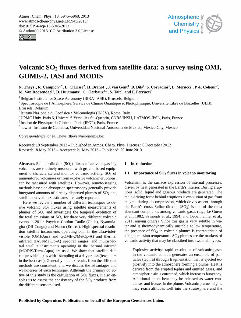
Fig. 2. (Left plot) Time series of SO2 total mass measured with IASI for the 2011 eruption of Puyehue-Cordon Caulle (blue dots). The redcurve is an exponential function fitted to the data (e-folding time: 6.8 days). A plume height of 13 km is assumed. (Right plot) Daily SO2fluxes calculated with the delta-M method applied to the total SO2 mass time series estimated on a half-daily and daily basis.
the eruption was continuing but as a result of their low in-tensity and altitude these emissions were below the detectionlimit of IASI retrievals. We fitted an exponential function tothe decay observed at the tail of the total SO2 mass curve re-sulting in an estimated e-folding lifetime of 6.8 days, typicalfor a dry atmosphere. Note that as the plume dilutes, partsof the plume will drop below the detection limit, so that thereal e-folding lifetime is probably a bit longer than what weestimate here.
From the SO2 mass time series, we then applied the delta-M method (Sect. 3.3) yielding SO2 fluxes averaged over atime interval1t (Eq. 6). The results are displayed in Fig. 2(right plot) for half-daily and daily mass estimates (1t = 1/2or 1 day). Note that the flux estimates for the first half-dayand first day have been calculated using a time interval of 7and 19 h, respectively (instead of 12 and 24 h), as it is more inline with the actual time between the start of the eruption andthe first observations. One can see in Fig. 2 that sometimesnegative fluxes are returned and that the fluxes time seriesare quite noisy (especially for the half-daily estimates). Thisis because the method relies on accurate estimates of consec-utive SO2 masses, which can be problematic for large anddispersed plumes. The erratic behavior of the half-day fluxeson 17 and 18 June is for instance due to the method usedfor a.m./p.m. differentiation which for these days causes por-tions of the plume to be counted twice. This behavior disap-pears when looking at the daily flux.
In addition to the simple delta-M method, Puyehue-Cordon Caulle was found to be an ideal case study to testthe traverse method (Sect. 3.2) because of the modest SO2loss term and because the SO2 injection occurred in a strongand well constrained wind field leading to steady and almostone-dimensional plumes (see Fig. 3). The analysis was madefor a sequence of four consecutive SO2 images right after thestart of the eruption; each time, the traverses were defined fora well-chosen portion of the plume (close to the volcano).
Following the traverse method formulation (Eq. 4), we cal-culate the SO2 fluxes using the MERRA wind fields (avail-able athttp://disc.sci.gsfc.nasa.gov/giovanni/overview/) ex-tracted at the location of the volcano and the time of observa-tions. It allows us to reconstruct a high-resolution chronologyof the SO2 flux during the eruption (Merucci et al., 2011).This is shown in Fig. 4, where the results from four consec-utive IASI snapshots (4 June p.m. to 6 June a.m.) are dis-played.
A striking feature is the fairly good overlap of the fluxdata for two successive overpasses, in spite of the constantwind field used in the calculation (for each IASI image). Thisclearly strengthens the adopted approaches. Note that for thefirst overpass, larger (and also more scattered) values are ob-served; this is probably due to the impact of ash (high con-centrations in the early plume) on the retrieved values.
Compared to the delta-M method (also shown on Fig. 4,for 1t = 1/2 day), results from the traverse method providemore information on the temporal variations of the emis-sions, in particular the peak occurring about 6 h after the be-ginning of the eruption, not seen with the lower time res-olution delta-M method. However, on average, the delta-Mand traverse methods give values that are consistent witheach other:∼ 180 kT day−1 on the first day then droppingto ∼ 60 kT day−1 on the second day.
In order to consolidate the flux results of Fig. 4, we havealso applied the inversion modeling method (Sect. 3.4) to thePuyehue-Cordon Caulle event. Since the injection heights arereasonably well known, we have used a small number of at-mospheric layers but worked at a high temporal resolution.More precisely, emission grid cells have been defined as 3layers of 1 km thickness from 11 to 14 km and 2-hourly in-tervals for the period 4–7 June 2011, starting at the onsetof the eruption. The FLEXPART simulations extended over3 days after each release period and the results are givenon a 0.5◦ × 0.5◦ output grid. Following the description in
www.atmos-chem-phys.net/13/5945/2013/ Atmos. Chem. Phys., 13, 5945–5968, 2013

5954 N. Theys et al.: Volcanic SO2 fluxes derived from satellite data
Fig. 3. SO2 columns from IASI measurements for 6 June 2011(morning overpass) over the Puyehue-Cordon Caulle volcano. Thelines correspond to the different traverses used for the SO2 fluxescalculation. A plume height of 13 km is assumed. The Puyehue-Cordon Caulle volcano is marked by a black triangle.
Sect. 3.4, a plume age dependent correction is applied usingan e-folding timeτ of 6.8 days (Fig. 2). The measurementvectory (Eq. 8) is assembled with the SO2 columns mea-sured by IASI (> 1 DU) for the period between 4 and 9 June2011 (daytime and nighttime overpasses) and evaluated onthe output grid. The vertical column calculation is made as-suming a plume height of 13 km. For the a priori emissions,a single value of 5 kT/2 h of SO2 is used for each emissiongrid cell to formxa . The a priori covariance matrixSa hasbeen chosen as diagonal with values corresponding to 250 %errors on the a priori emissions. For the observation error co-variance matrixSε, a diagonal matrix has been chosen andwe assumed a conservative 50 %+ 1 DU uncertainty on themeasurements.
The inversion results are displayed in Fig. 4 (grey bars),where the a posteriori emissions have been vertically inte-grated and scaled to yield SO2 fluxes. Overall, the results ofFig. 4 are very positive as they show that, for the case ofPuyehue-Cordon Caulle, it is possible to resolve the volcanicSO2 emissions with a time step as short as∼ 2 h. One cansee that there is a very good correspondence between the re-sults of the traverse and inversion modeling methods, whichstrengthens both approaches.
By integrating the fluxes of Fig. 4, we estimate the totalSO2 mass released by Puyehue-Cordon Caulle during thefirst two days of eruption to be about 200 kT. However, thisestimate is a lower bound as it does not include the contribu-tion of SO2 emitted at lower altitude.
As an illustration of the inversion modeling method, Fig. 5shows daily SO2 column maps retrieved from IASI and sim-
Fig. 4.SO2 flux evolution through the first two days of the Puyehue-Cordon Caulle eruption obtained from the traverse method (analy-sis of four consecutive IASI images) and compared to the delta-M(1t = 1/2 day; pale orange bars) and inversion modeling methods(grey bars).
ulated by FLEXPART using the retrieved emissions (K · x),for 6 and 7 June 2011. As can be seen, a fair agreement isfound between IASI and FLEXPART both for the dispersionpatterns and the absolute SO2 column values.
4.2 Nyamulagira
Nyamulagira (1.41◦ S, 29.20◦ E, 3058 m a.s.l.) erupted over40 times in the last century, and is known to be one of themain sources of volcanic SO2 worldwide (Carn et al., 2003).Based on TOMS measurements, the SO2 output from Nya-mulagira has been monitored during the 1979–2005 period,and a majority of eruptions produced more than 0.8 MT ofSO2 (Bluth and Carn, 2008).
Almost two years after the last eruption of 2–29 January2010, Nyamulagira started erupting again, on 6 November2011 (18:45 UTC) with observed lava fountains reaching upto 300 m and with large amounts of SO2 easily detected fromspace. The eruption lasted five months, until 15 March 2012.
For several weeks, the plume of SO2 was monotonicallydrifting westward from the volcano (as illustrated in the insetin Fig. 6); its altitude was between 4 and 8 km (based on winddirection data from ECMWF).
We investigated the 2011–2012 Nyamulagira eruption forthe first month (when the signal was the strongest) using theUV sensors (OMI and GOME-2) as they are the most suitableto monitor this event owing to their good sensitivity down tothe surface. A strong signal of SO2 could also be detectedwith IASI especially at the beginning of the eruption, but thedata are more difficult to use because of increasing errors onthe columns with decreasing plume altitude (the plume ofSO2 was low in the atmosphere).
Atmos. Chem. Phys., 13, 5945–5968, 2013 www.atmos-chem-phys.net/13/5945/2013/

N. Theys et al.: Volcanic SO2 fluxes derived from satellite data 5955
Fig. 5.SO2 columns measured by IASI (evening overpasses) and simulated by FLEXPART using the a posteriori emissions from the inversionfor 6 June 2011 (left panels) and 7 June 2011 (right panels). The measured columns are averaged over the 0.5◦
× 0.5◦ FLEXPART output.The simulated columns are (1) calculated from the SO2 profiles weighted by the corresponding altitude-dependent measurement sensitivityfunctions (averaging kernels) and (2) interpolated at the time of observations. The Puyehue-Cordon Caulle volcano is marked by a blacktriangle.
Fig. 6.OMI daily SO2 mass as function of plume age (see text) av-eraged for November 2011. The inset shows the monthly averagedSO2 columns measured by OMI above Nyamulagira for November2011.
Since the plume altitude is not known exactly, we sim-ply took the available middle tropospheric altitude (centerof mass heights of 6 and 7.5 km for GOME-2 and OMI,respectively) for the SO2 vertical column calculation. Thisassumption is a source of uncertainty but the effect onthe SO2 columns is modest, with errors lower than 30 %(Fig. 1). In order to isolate the volcanic SO2 signal from thebackground noise, an SO2 column threshold was assigned(VC > VClim = VC+3·σVC), using the mean (VC) and stan-dard deviation (σVC) of daily SO2 VCs retrieved in the back-ground region (Carn et al., 2008).
As already mentioned, the SO2 plumes from Nyamulagirahad a rather simple geometry owing to fairly stable meteo-rological conditions. This situation facilitates the calculationof the loss term (see e.g., Beirle et al., 2011) and of the SO2fluxes. The first loss term has been estimated from the decayobserved in the total SO2 mass downwind (westward) of thevolcano. This is illustrated in Fig. 6 showing the averagedSO2 mass for November 2011 as a function of plume age,expressed in hours.
The values are calculated using daily OMI SO2 columnsintegrated along traverses perpendicular to the wind vector.The plume age is the ratio of the distance (defined as pos-itive downwind) between a given pixel and the volcano andthe wind speed. For each day, the wind vector is derived from
www.atmos-chem-phys.net/13/5945/2013/ Atmos. Chem. Phys., 13, 5945–5968, 2013

5956 N. Theys et al.: Volcanic SO2 fluxes derived from satellite data
Fig. 7. Time series of SO2 total mass measured with OMI for the2011 eruption of Nyamulagira. Shown are the daily values (grey),5-day moving averages (black) and a skewed shape function fittedto the smoothed curve (red).
the visual analysis of the transport direction of the plume andcomparison with the 1◦ × 1◦ ECMWF 24 h averaged profile(closest to the volcano) of wind direction and speed. FromFig. 6, the fitting of an exponential function (red curve) tothe SO2 mass data is straightforward and yields a mean SO2e-folding time of 22.5 h, in good agreement with the litera-ture (Bluth and Carn, 2008). Moreover, we repeated the sameanalysis using GOME-2 data and obtained a consistent valueof 24.9 h.
Having reasonably accurate values of the SO2 loss termfor both OMI and GOME-2, we can estimate the fluxes usingsome of the methods described in Sect. 3. We start to applythese methods to the data from OMI as it is the instrumentwith the most favorable spatial resolution and noise level.
We first used the delta-M method. Similarly to the analysisof the Puyehue-Cordon Caulle eruption, it is applicable to thedaily SO2 mass values (Fig. 7, grey bars) and does not requireinformation on the daily wind fields.
We also tested the skewed shape method (Sect. 3.3). Sinceit implies the adjustment of a continuous and regular func-tion (Eq. 7), we applied this method to the (smoothed) 5-daymoving averages SO2 mass time series (Fig. 7, black stemswith the fitted curve in red).
The resulting fluxes are shown in Fig. 8 for both methods.
Also shown in Fig. 8, are the results from the box(Sect. 3.1) and traverse (Sect. 3.2) methods. For the boxmethod, we selected the days for which the SO2 plume hada simple geometry, was well covered by the satellite instru-ment and when the wind speed was not anomalously highor low. We calculated a daily flux (Fig. 8, blue bars) basedon the data contained in a circle around the volcano, witha radius changing each day depending on the wind speed.
Fig. 8. Daily SO2 fluxes derived from different methods applied toOMI data for the first month of the 2011 eruption of Nyamulagira.
For the traverse method, daily values (Fig. 8, pink squares)were calculated whenever possible by averaging the fluxesover the closest five to ten traverses (excluding the first onebecause of sub-pixel dilution issues). Note that the recon-struction of short-term variations of the flux, as for Puyehue-Cordon Caulle, was found difficult. Short and variable SO2lifetime, as well as a poorly constrained wind field far awayfrom the volcano makes this kind of approach too uncertainin this case.
In general, the retrieved SO2 fluxes from the differentmethods are found to be in reasonable agreement, all show-ing large values (40–230 kT day−1) for the first week of theeruption and then a flattening afterwards (10–30 kT day−1)reflecting a calmer eruptive regime. In total, we estimate theSO2 amount produced by Nyamulagira during the first monthof eruption to be of about 1 MT.
Compared to the other methods, the delta-M methodshows more variable and uncertain results. This is mainlybecause the plume is often not completely covered by OMIfor two consecutive days. Now comparing the results of theskewed shape, box and traverse methods, the differences ob-served can be explained by small differences in selection ofdata, details in the settings and uncertainties on the windspeed.
To consolidate the results, we also analyzed the GOME-2SO2 data using the same techniques as for OMI. The resultsare displayed in Fig. 9, together with the OMI fluxes. Onlythe data from the circle and skewed shape methods are shownfor better readability.
A general consistency is found between OMI and GOME-2 results, although GOME-2 has a tendency to producehigher values than OMI (probably because of differences inthe treatment of clouds in the retrievals and in meteorologicalconditions). As these results are in principle independent of
Atmos. Chem. Phys., 13, 5945–5968, 2013 www.atmos-chem-phys.net/13/5945/2013/

N. Theys et al.: Volcanic SO2 fluxes derived from satellite data 5957
Fig. 9. Time series of Nyamulagira SO2 fluxes retrieved from thebox (bars) and skewed shape (lines) methods applied to OMI andGOME-2 data.
the pixel size, they constitute however a valuable element ofsuccessful satellite–satellite comparison, complementing ex-isting SO2 flux comparison exercises (e.g., Campion, 2011;and Campion et al., 2012).
Finally, it is important to note that, at the beginning of theevent, the SO2 fluxes (Figs. 8, 9) could be underestimatedbecause of SO2 absorption saturation. However, from the in-spection of the SO2 column values, we believe the effect onthe fluxes is small, with differences lower than 10 %.
In an attempt to ascertain a reasonable uncertainty onthe derived fluxes, we conducted sensitivity tests by vary-ing the different important parameters of the retrieval. Basedon these sensitivity tests, a typical error for both OMI andGOME-2 estimates is of about 50 %, and includes the uncer-tainties on the SO2 columns, cutoff values used, SO2 lossesand wind fields.
4.3 Nabro
Nabro (13.37◦ N, 41.70◦ E, 2218 m a.s.l.) is located in theAfrican rift zone at the border between Eritrea and Ethiopia.In spite of no reported historical eruptions, Nabro erupted inthe evening of 12 June 2011 around 20:30 UTC, expellinga powerful plume composed of enormous amounts of steamand SO2, with little amounts of ash. At the beginning of theeruption, SO2 was massively injected at tropical tropopauselevels where fast easterly jet winds (∼ 30 m s−1) transportedthe plume towards the Mediterranean Middle East and, later,to China. Less powerful, the next phase of the eruption in-jected SO2 at lower altitudes but still the dispersion of theplume occurred over a large part of the African continent.
The eruption led to a∼ 20 km-long lava flow in lessthan ten days (seehttp://earthobservatory.nasa.gov/). It lastedabout one month; remnants of volcanic SO2 could still be
observed by the UV sensors on 17 July 2011. The compar-ison of satellite UV and TIR SO2 images revealed inhomo-geneous multi-layered SO2 plumes dispersed over large dis-tances, making the SO2 fluxes calculation a complex prob-lem to solve. Therefore we have used a more elaborated ap-proach: the inverse modeling method (Sect. 3.4).
Note that Nabro is a difficult event to analyze as – un-like the Puyehue-Cordon Caulle (explosive) and the Nyamu-lagira (effusive) eruptions discussed above – it fundamen-tally was an effusive eruption releasing an exceptional gasjet that reached the tropopause prior to strong lava emis-sion. As there is no evidence that this plume was ash ladenas would be expected of a high altitude plume, Nabro re-mains an intriguing, atypical example in this respect. Thetransport mechanism of the initial Nabro eruption plume isalso peculiar. Bourassa et al. (2012) have suggested deepconvection associated with the Asian monsoon circulationto explain the strong impact of the eruption on the strato-spheric aerosol loading. However, this mechanism is contro-versial after Vernier et al. (2013) and Fromm et al. (2013)provided satellite evidence for direct injection of the initialNabro plume into the lower stratosphere.
4.3.1 Inversion settings
The inversion of the time-dependent SO2 emission profilesis based on the maximum a posteriori solution described inSect. 3.4 (Eq. 10). The emission grid cells are defined as: 16layers of 1 km thickness from 2 to 18 km altitude and 64 6-hourly intervals for the period 13–28 June 2011, plus an addi-tional profile to cope with the plume for the very first hours ofthe eruption (12 June – 20:30 UTC to 13 June – 00:00 UTC).The inversion consists in estimating the SO2 masses that havebeen emitted in each of these grid cells. In line with Eq. (8),we define a state vectorx that gathers all then = 1040 un-known emissions.
The FLEXPART simulations extended over 5 days aftereach release period and the results are given on a 1◦
× 1◦
output grid. As mentioned in Sect. 3.4, concentrations are in-terpolated in space and time with the satellite measurements(see below), multiplied by the corresponding SO2 averagingkernels (to allow direct comparisons with satellite measure-ments) and vertically integrated to provide columns. For thepresent study, we have applied a correction for SO2 loss us-ing aτ value different for each emission layer. From the de-cay observed in the total SO2 mass after the end of the firstmajor injection episode (not shown), we derive an e-foldinglifetime of 5 days for the high altitude plumes at 15–18 km(Vernier et al., 2013; Fromm et al., 2013). The e-folding timeparameterization as a function of altitude was estimated byinterpolation between the values at surface level, taken as 2days, and the one at 15–18 km (5 days). The value of the SO2e-folding time at the surface has been varied until the bestmatch was found between the measurements and the simula-tions.
www.atmos-chem-phys.net/13/5945/2013/ Atmos. Chem. Phys., 13, 5945–5968, 2013

5958 N. Theys et al.: Volcanic SO2 fluxes derived from satellite data
Fig. 10.SO2 columns measured by IASI (morning overpass) and GOME-2 and simulated by FLEXPART using the a posteriori emissionsfrom the inversion for 15 June 2011(a), 16 June 2011(b), 18 June 2011(c) and 20 June 2011(d). The measured columns are averagedover the 1◦ × 1◦ FLEXPART output grid. The simulated columns are (1) calculated from the SO2 profiles weighted by the correspondingaltitude-dependent measurement sensitivity functions (averaging kernels) and (2) interpolated at the time of observations. The Nabro volcanois marked by a black triangle. The orange box shows the SO2 plume released in the first 15 h of the eruption.
The observations used to build the measurement vectory
(Eq. 8) are the SO2 columns measured by IASI (daytime andnighttime overpasses) and GOME-2 for the period between13 June and 3 July 2011, evaluated on the output grid. Notehowever that the GOME-2 measurements for 14 June 2011have not been considered in the analysis because the instru-ment was operating in its narrow swath mode on that day.
As a baseline, the calculation is made for SO2 columnslarger than 1 DU and assuming a plume height of 16 km forboth sensors. Hence the averaging kernels by definition equal1 at this altitude.
To solve the inversion problem (Eq. 10), several othervariables need to be specified: the a priori state vector(xa), the error covariance matrices of the a priori (Sa) andof the measurements (Sε). For the a priori emissions, we
Atmos. Chem. Phys., 13, 5945–5968, 2013 www.atmos-chem-phys.net/13/5945/2013/

N. Theys et al.: Volcanic SO2 fluxes derived from satellite data 5959
have estimated first-order SO2 flux from the skewed shapedmethod (Sect. 3.3) applied to the global SO2 total mass timeseries from GOME-2 (i.e., with a measurement sensitivity toSO2 down to the surface). For each day, the inferred SO2mass was then distributed equally in each emission grid cellto form xa. The a priori covariance matrixSa has been cho-sen diagonal with values corresponding to 250 %+ 2 kT er-rors on the a priori emissions, except in the layers below 6 kmwhere a larger uncertainty was used (2000 %+ 10 kT of thea priori emissions). Based on sensitivity tests, these settingswere adopted to avoid an inversion over-constrained by thea priori values because of reduced sensitivity to SO2 in thelower troposphere. For the observation error covariance ma-trix Sε, a diagonal matrix has been chosen and we assumed aconservative 50 %+ 1 DU uncertainty on the measurements.Note that we tested the sensitivity of the inversion to the ob-servation error covariance matrixSε and it was found to bereasonably small.
4.3.2 Results
From inspection of the SO2 column distributions, it appearsthat the GOME-2 and IASI data are quite similar, but thesequence of SO2 images also shows differences that can beattributed (at least partly) to plumes of SO2 at different al-titudes. In principle, the inversion scheme exploits the in-strumental complementarities to resolve the injection pro-files in the altitude range extending from the surface to thelower stratosphere. At the beginning of the eruption, SO2 ismassively injected at high altitudes and the IASI retrieval isfound to be optimal, owing to its large column applicabilityand 12 h revisiting time (as opposed to 24 h for GOME-2).Shortly after the first injection episode, SO2 is more evenlydistributed throughout the atmosphere, conditions for whichGOME-2 provides information on the total atmospheric SO2column, including the contribution from the lower tropo-sphere (not probed as efficiently by IASI). Note that afterthe first week of the eruption, the IASI SO2 signal close toNabro is quite small, indicating low altitude SO2 plumes andhence most information on the emissions is brought by theGOME-2 data.
Before inspecting the inverted fluxes, let us first comparethe SO2 columns retrieved from GOME-2 or IASI and sim-ulated by FLEXPART using the retrieved emissions. As anillustration, Fig. 10 shows daily SO2 maps for 15, 16, 18 and20 June 2011.
Generally the simulated SO2 vertical columns agree fairlywell with the observations. However, it should be noted thatthe strong SO2 plume released at the beginning of the erup-tion, which then moves towards East Asia, is not well repro-duced by the simulations. This plume was injected at highaltitudes in the first 15 h of eruption. The reasons for this dis-crepancy will be investigated in Sect. 4.3.3. Nevertheless, theoverall good agreement between the observed and modeledSO2 columns for the other plumes suggests that it is neither
Fig. 11.Comparison of SO2 flux estimates for the eruption of Nabrousing different methods. Upper panel: vertically integrated a pos-teriori emissions from the inversion combining IASI and GOME-2 data (dark grey bars:> 6 km; light+ dark grey bars: total flux),flux estimate of the early plume using the box method applied toIASI (orange bar; see text and Fig. 10a), results of the skewed-shape method applied to GOME-2 data and used as a priori in theinversion (blue dotted line;z: 16 km), results of the delta-M methodapplied to IASI data (magenta and red lines for half-daily and dailymass estimates;z: 16 km) and results of the traverse method appliedto MODIS (cyan squares). Lower panel: same as upper panel (butwith a focus on the first four days of eruption) with flux results ofthe traverse method for three IASI images at the beginning of theeruption.
a serious nor a general problem. From Fig. 10, one can alsosee that not all plume maxima are well captured. This pointsto limitations in the approach used (in terms of spatial andtime resolution) to capture the complexity and details of theemissions (Eckhardt et al., 2008).
The flux estimates are displayed in Fig. 11 (upper panel),where the a posteriori emissions have been integrated
www.atmos-chem-phys.net/13/5945/2013/ Atmos. Chem. Phys., 13, 5945–5968, 2013

5960 N. Theys et al.: Volcanic SO2 fluxes derived from satellite data
vertically (from 2 to 18 km: sum of dark and light grey bars)and in time to yield daily SO2 fluxes. As an illustration,Fig. 11 (upper panel) also shows the a posteriori fluxes forthe 6–18 km altitude range (dark grey bars), the a priori fluxes(Sect. 4.3.1) and the results from other methods (see discus-sion below).
From Fig. 11, several remarks can be made.
1. It is important to mention that, although it helps min-imizing the cost functionJ (Eq. 9), working with anemission time step of 6 h may also be problematic insome cases, because the satellite revisit time is 12 h atbest. This is particularly true for plumes at low altitudewhere the wind speed is modest and the SO2 loss pro-cesses are fast. Consequently, the variability of the in-verted emissions should not be strictly interpreted, astwo consecutive values are likely too correlated. There-fore, we have recalculated the SO2 emissions on a dailybasis (more stable in time).
2. Accurate simulation of the transport of SO2 was chal-lenging for the plume released in the first 15 h of erup-tion. The corresponding inversion results are uncertain(because of misfit effects), and to estimate the SO2 fluxfor the early injection we have applied the box method(see Sect. 3.1). Based on the FLEXPART simulations, itwas possible to identify what part of the observed plumewas released during the first 15 h (the plume in the or-ange box in Fig. 10a). By using moving boxes for threeconsecutive IASI overpasses (from 14 June a.m. to 15June a.m. 2011), we calculated an averaged total SO2mass released in the first 15 h and hence an SO2 flux(Fig. 11 – orange bar) by applying a factor accountingfor the SO2 decay since the release.
3. In contrast to the fluxes from the skewed shape method(a priori fluxes), which are generally too low, the fluxesfrom the inversion modeling method (Fig. 11, upperpanel) clearly reveal two volcanic regimes. In the firstfour days of eruption, large values of the fluxes (500–950 kT day−1) are observed and SO2 is vertically dis-tributed throughout the entire atmosphere (2–18 kmrange), except probably for the very early plume whereheights are mostly in the 15–18 km range. On 17 June2011 substantially lower fluxes (80–250 kT day−1) areobserved and SO2 plumes are mostly below 6 km. Thissecond phase of the eruption is mostly effusive (seeSect. 1.1). It should be noted that the retrieved emis-sions in the lower troposphere for 13–14 June 2011have higher uncertainties. This is essentially because theGOME-2 instrument was operating in its narrow swathmode on 14 June 2011 and no useful data was availableon that day.
4. The delta-M method (Sect. 3.3) was applied to IASIcolumns (assuming a plume height of 16 km). One can
see that the results (displayed in Fig. 11, magenta andred lines) capture nicely the large SO2 flux at the startof the eruption and then agree well with the fluxes forthe layers in the 6–18 km altitude range. After 20 June,the IASI signal becomes small and the delta-M methodreturns negative values, because of errors in the IASIretrievals and assumed SO2 e-folding time. For the firsttwo days of eruptions (13–14 June 2011), it was possi-ble to apply the traverse method (Sect. 3.2) to portionsof plumes measured by IASI. The results are shown inthe lower panel in Fig. 11, which is a zoom on the firstfour days of the eruption. The results agree fairly wellwith the flux estimates in the 6–18 km range (whereIASI has a good sensitivity to SO2). Moreover, the re-sults from the traverse method enable us to consolidatethe flux results at the very beginning of the eruption(early plume).
5. The SO2 fluxes have also been estimated by applyingthe traverse method (Sect. 3.2) to MODIS measure-ments. The pressure, temperature and humidity profiles,needed for the SO2 retrieval computation (see Sect. 2.4),derive from ECMWF data considering a 3◦
× 3◦ gridaround Nabro. The plume axes direction and the windspeed have been extracted from the ECMWF profiles atthe plume altitude. By exploiting the high spatial reso-lution of MODIS, the mean SO2 flux has been estimatedin the region lying in the first 300 km from the volcanicvent (also to avoid the depletion of SO2 since its re-lease). Note that the MODIS TIR images for 13 and 16June show a strong absorption due to condensed watervapor. Such particles absorb in the entire TIR spectralrange and this leads to an overestimation of the SO2 to-tal amount. To account for this effect a correction for thewater vapor content has been applied. The procedure isbased on the same approach described by Corradini etal. (2009) to correct for ash but adapted here for watervapor optical properties (as input of the radiative trans-fer code). As can be seen, the MODIS fluxes do agreereasonably well with the estimates presented above.
6. From Fig. 11, we estimate the total SO2 mass releasedby Nabro during the first fifteen days of eruption to beof about 4.5 MT.
7. We conducted test retrievals to estimate the uncertaintyon the fluxes displayed in Fig. 11. A reasonable value ofthe total error is of about 50 %.
4.3.3 Discussion
Transport of the early plume
We now explore the reasons for the differences betweenthe observations and the FLEXPART simulated patterns. Asmentioned above, the large SO2 plume at the beginning of
Atmos. Chem. Phys., 13, 5945–5968, 2013 www.atmos-chem-phys.net/13/5945/2013/

N. Theys et al.: Volcanic SO2 fluxes derived from satellite data 5961
IASI
FLEXPART (a posteriori)
16.06.2011 14.06.2011
[DU]
FLEXPART (a posteriori)
IASI
FLEXPART
(sensitivity test)
0° 30°E 60°E
0°
30°N
0° 60°N
30°E 60°E
0°
[DU]
30°N
45°E 60°N
95°E 145°E
0°
30°N
45°E 60°N
95°E 145°E
0°
30°N
45°E 60°N
95°E 145°E
0°
30°N
60°N
Fig. 12.Comparison of SO2 columns measured by IASI (morning overpass) and simulated by FLEXPART using the a posteriori emissionsfrom the inversion for 14 (left) and 16 June 2011 (right). Also shown is a map of the SO2 columns simulated by FLEXPART for 16 June2011 using (as a sensitivity test) the IASI observations on 14 June 2011 as sources elements (see text).
the eruption was poorly constrained by the inversion. Thisleads to an underestimation of the modeled SO2 columns asillustrated in Figs. 10 and 12 (left and center plots).
There are several possible explanations for this feature(see discussion by Eckhardt et al., 2008). One possibility isthat errors on the high altitude wind fields propagate withtime making the transport simulation uncertain. To test thishypothesis, we have run FLEXPART using different windfields; namely the National Centers for Environmental Pre-diction (NCEP) Global Forecast System (GFS) analyses with1◦
× 1◦ resolution. It emerged from sensitivity tests that thesimulated dispersion patterns were close to the original data.Another option to explain the discrepancy between the ob-servations and the simulations is to consider an effect fromthe eruption itself. It could be that for the early phase ofthe eruption the assumption of a passively advected plumeis not fulfilled anymore. Discrepancies may arise from radia-tive heating of the plume (e.g., leading to self-lofting of theplume; Eckhardt et al., 2008), gas trapping in ice or becauseof water vapor conversion to ice (Textor et al., 2003). To testthis assumption, we have made a sensitivity test illustrated inFig. 12. Using the a posteriori emissions, one can see that thesimulated columns strongly deviate from the correspondingIASI SO2 columns for 14 and 16 June 2011. If the observed
discrepancies are due to the action of the plume, it is reason-able to assume that several hours after the start of the eruption(12 June 2011 around 20:30 UTC) the physical and chemi-cal processes that occurred in-situ have stopped, so that theplume can be considered as passive again. As a test, we haverun a FLEXPART simulation starting on 14 June 2011 (i.e.,more than 30 h after the start of the eruption) using the IASISO2 observations as emission cells, the source strengths be-ing modulated by the corresponding measured SO2 masses.Only the data with latitudes above 20◦ N have been kept andthe simulations assumed a uniform SO2 profile between 15and 18 km (Vernier et al., 2013; Fromm et al., 2013). The re-sults are shown in Fig. 12 (right plot) on 16 June 2011 at thetime of IASI measurements (morning overpass). One can seethat, compared to the modeled columns using the a posterioriemissions, the simulated columns are much closer to the IASIobservations. The fact that the pattern extending from WestMongolia to central China could be reasonably well repro-duced indicates that the wind data are compatible with thereal dispersion of the plume. This suggests that the differ-ences between the observations and the original FLEXPARTsimulations are due – at least partly – to the action of theplume released in the first hours of the eruption.
www.atmos-chem-phys.net/13/5945/2013/ Atmos. Chem. Phys., 13, 5945–5968, 2013

5962 N. Theys et al.: Volcanic SO2 fluxes derived from satellite data
More work is needed to study the transport of the NabroSO2 plume and to ascertain the importance of the Asian mon-soon circulation in the uplift of this plume (Bourassa et al.,2012).
Intercomparison of GOME-2 and IASI
As shown in Sect. 4.3.2, the inversion modeling method ap-plied to the eruption of Nabro provides good results. How-ever, the technique implicitly assumes that the SO2 columnsfrom GOME-2 and IASI are compatible with each other, inthe sense that differences in the column amount are only dueto deviations from the actual plume height (Fig. 1). The aimof this section is to investigate whether this assumption isfulfilled.
In a first step, we used the information on the SO2 plumeheights provided by the a posteriori FLEXPART simulations.For this purpose, we calculate, at each time step and for eachgrid point, the height of the SO2 center of mass using the op-timized (non-zero) SO2 concentration profiles. The retrievedSO2 heights are then used to investigate the consistency ofthe SO2 column datasets from GOME-2 and IASI. However,this analysis is only possible if the plume altitudes returnedby the simulations are reliable enough. Therefore, we havemade comparisons with independent altitude estimations ob-tained with collocated GOME-2 observations, to assess theaccuracy of the modeled plumes heights. Here the effec-tive height of the SO2 plume is retrieved from the GOME-2 backscattered radiance measurements using a direct fittingapproach (van Gent et al., 2013; Yang et al., 2010; Nowlanet al., 2011). An example of comparison in a region close toNabro for 16 June 2011 is displayed in Fig. 13.
From the GOME-2 and FLEXPART SO2 plume height im-ages in Fig. 13, we found that both data are able to capture acomplex situation with two SO2 plumes at different altitudes:a plume at 3–5 km transported to the south and another plumeat 8–12 km drifting westward of the volcano. More quantita-tively, the modeled and observed plume heights are found tobe in good agreement, with differences in the 1–2 km range.Although it does not constitute a proper validation, the com-parison of Fig. 13 tends to consolidate the inverted emissionsand related plume height estimations.
Next we compare the GOME-2 and IASI SO2 data by ac-counting for the effect of altitude. This was achieved by inter-polating the averaging kernels (estimated for each GOME-2and IASI measurement; Fig. 1) at the corresponding FLEX-PART SO2 plume heights. The calculation supplies conver-sion factors that are then applied to the respective verticalcolumns from both sensors. For the conditions where no in-formation on the altitude was available, we took the plumeheight value from the closest grid point to the correspondingmeasurement.
Figure 14 shows time series of SO2 masses for the firstfifteen days of the eruption of Nabro using the recalculatedGOME-2 and IASI vertical columns.
Fig. 13.Comparison of SO2 plume height retrieved from GOME-2spectra using a direct fitting approach (left) and simulated by FLEX-PART using the a posteriori emissions (right) for 16 June 2011 inthe vicinity of Nabro.
The upper panel in Fig. 14 shows the GOME-2 total SO2masses as a function of time, for different selection criteria onthe data. The black curve sums the SO2 amount for all plumeheight scenarios from the surface to lower stratospheric lay-ers, while the red curve only considers the data with SO2plume heights above 6 km. One can see that the agreementbetween GOME-2 (red curve) and IASI (blue curve) SO2masses is remarkable when the comparison is restricted toplumes in the altitude range where IASI is sensitive (> 6 km).The differences between IASI and GOME-2 masses are mostof the time lower than 25 %. To rule out possible compensa-tion effects, we have also compared the GOME-2 and IASItime series of SO2 masses separately for different altituderanges: 6–9, 9–12 and above 12 km. The results are displayedin Fig. 14 (lower panel). Again, the GOME-2 and IASI SO2masses data are in excellent agreement.
These results strengthen the inversion modeling approachpresented in Sects. 4.3.1 and 4.3.2 and also confirm that thelargest errors on the UV and TIR SO2 columns is the errormade by assuming a wrong SO2 altitude.
One can argue that for individual scenes the discrepan-cies between GOME-2 and IASI can be much higher thanwhat has been presented here, because of saturation issues.Indeed, the GOME-2 DOAS retrieval tends to underestimatethe SO2 amount for columns larger than 50–100 DU, whereasthe IASI algorithm is designed to cope with nonlinear effectsdue to a large SO2 amount (Clarisse et al., 2012). However,from the inspection of the SO2 columns (measured by IASI),we believe this translates to small differences for the timeseries shown in Fig. 14 because this saturation effect onlyaffects a small number of pixels, those with the highest SO2concentrations (at the beginning of the time series). Note thatthe plume may also contain large amounts of aerosols (no-tably ice) and gases (e.g., water vapor) all absorbing or scat-tering the photons differently depending on the wavelength.This can also cause differences between the UV and TIRSO2 data (again mostly at the beginning of the time series),
Atmos. Chem. Phys., 13, 5945–5968, 2013 www.atmos-chem-phys.net/13/5945/2013/
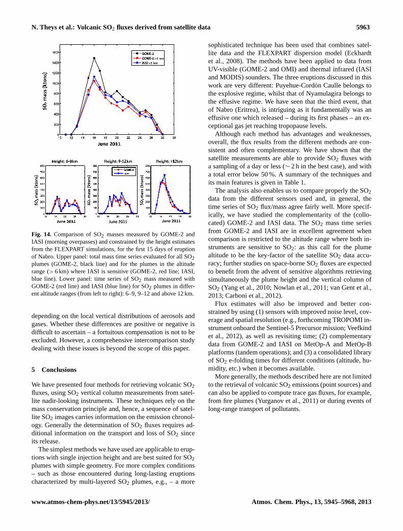
N. Theys et al.: Volcanic SO2 fluxes derived from satellite data 5963
Fig. 14. Comparison of SO2 masses measured by GOME-2 andIASI (morning overpasses) and constrained by the height estimatesfrom the FLEXPART simulations, for the first 15 days of eruptionof Nabro. Upper panel: total mass time series evaluated for all SO2plumes (GOME-2, black line) and for the plumes in the altituderange (> 6 km) where IASI is sensitive (GOME-2, red line; IASI,blue line). Lower panel: time series of SO2 mass measured withGOME-2 (red line) and IASI (blue line) for SO2 plumes in differ-ent altitude ranges (from left to right): 6–9, 9–12 and above 12 km.
depending on the local vertical distributions of aerosols andgases. Whether these differences are positive or negative isdifficult to ascertain – a fortuitous compensation is not to beexcluded. However, a comprehensive intercomparison studydealing with these issues is beyond the scope of this paper.
5 Conclusions
We have presented four methods for retrieving volcanic SO2fluxes, using SO2 vertical column measurements from satel-lite nadir-looking instruments. These techniques rely on themass conservation principle and, hence, a sequence of satel-lite SO2 images carries information on the emission chronol-ogy. Generally the determination of SO2 fluxes requires ad-ditional information on the transport and loss of SO2 sinceits release.
The simplest methods we have used are applicable to erup-tions with single injection height and are best suited for SO2plumes with simple geometry. For more complex conditions– such as those encountered during long-lasting eruptionscharacterized by multi-layered SO2 plumes, e.g., – a more
sophisticated technique has been used that combines satel-lite data and the FLEXPART dispersion model (Eckhardtet al., 2008). The methods have been applied to data fromUV-visible (GOME-2 and OMI) and thermal infrared (IASIand MODIS) sounders. The three eruptions discussed in thiswork are very different: Puyehue-Cordon Caulle belongs tothe explosive regime, whilst that of Nyamulagira belongs tothe effusive regime. We have seen that the third event, thatof Nabro (Eritrea), is intriguing as it fundamentally was aneffusive one which released – during its first phases – an ex-ceptional gas jet reaching tropopause levels.
Although each method has advantages and weaknesses,overall, the flux results from the different methods are con-sistent and often complementary. We have shown that thesatellite measurements are able to provide SO2 fluxes witha sampling of a day or less (∼ 2 h in the best case), and witha total error below 50 %. A summary of the techniques andits main features is given in Table 1.
The analysis also enables us to compare properly the SO2data from the different sensors used and, in general, thetime series of SO2 flux/mass agree fairly well. More specif-ically, we have studied the complementarity of the (collo-cated) GOME-2 and IASI data. The SO2 mass time seriesfrom GOME-2 and IASI are in excellent agreement whencomparison is restricted to the altitude range where both in-struments are sensitive to SO2: as this call for the plumealtitude to be the key-factor of the satellite SO2 data accu-racy; further studies on space-borne SO2 fluxes are expectedto benefit from the advent of sensitive algorithms retrievingsimultaneously the plume height and the vertical column ofSO2 (Yang et al., 2010; Nowlan et al., 2011; van Gent et al.,2013; Carboni et al., 2012).
Flux estimates will also be improved and better con-strained by using (1) sensors with improved noise level, cov-erage and spatial resolution (e.g., forthcoming TROPOMI in-strument onboard the Sentinel-5 Precursor mission; Veefkindet al., 2012), as well as revisiting time; (2) complementarydata from GOME-2 and IASI on MetOp-A and MetOp-Bplatforms (tandem operations); and (3) a consolidated libraryof SO2 e-folding times for different conditions (altitude, hu-midity, etc.) when it becomes available.
More generally, the methods described here are not limitedto the retrieval of volcanic SO2 emissions (point sources) andcan also be applied to compute trace gas fluxes, for example,from fire plumes (Yurganov et al., 2011) or during events oflong-range transport of pollutants.
www.atmos-chem-phys.net/13/5945/2013/ Atmos. Chem. Phys., 13, 5945–5968, 2013
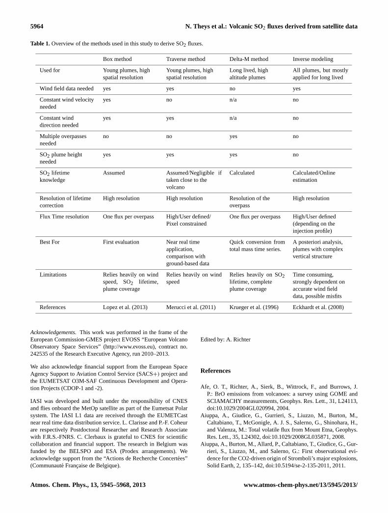
5964 N. Theys et al.: Volcanic SO2 fluxes derived from satellite data
Table 1.Overview of the methods used in this study to derive SO2 fluxes.
Box method Traverse method Delta-M method Inverse modeling
Used for Young plumes, highspatial resolution
Young plumes, highspatial resolution
Long lived, highaltitude plumes
All plumes, but mostlyapplied for long lived
Wind field data needed yes yes no yes
Constant wind velocityneeded
yes no n/a no
Constant winddirection needed
yes yes n/a no
Multiple overpassesneeded
no no yes no
SO2 plume heightneeded
yes yes yes no
SO2 lifetimeknowledge
Assumed Assumed/Negligible iftaken close to thevolcano
Calculated Calculated/Onlineestimation
Resolution of lifetimecorrection
High resolution High resolution Resolution of theoverpass
High resolution
Flux Time resolution One flux per overpass High/User defined/Pixel constrained
One flux per overpass High/User defined(depending on theinjection profile)
Best For First evaluation Near real timeapplication,comparison withground-based data
Quick conversion fromtotal mass time series.
A posteriori analysis,plumes with complexvertical structure
Limitations Relies heavily on windspeed, SO2 lifetime,plume coverage
Relies heavily on windspeed
Relies heavily on SO2lifetime, completeplume coverage
Time consuming,strongly dependent onaccurate wind fielddata, possible misfits
References Lopez et al. (2013) Merucci et al. (2011) Krueger et al. (1996) Eckhardt et al. (2008)
Acknowledgements.This work was performed in the frame of theEuropean Commission-GMES project EVOSS “European VolcanoObservatory Space Services” (http://www.evoss.eu), contract no.242535 of the Research Executive Agency, run 2010–2013.
We also acknowledge financial support from the European SpaceAgency Support to Aviation Control Service (SACS+) project andthe EUMETSAT O3M-SAF Continuous Development and Opera-tion Projects (CDOP-1 and -2).
IASI was developed and built under the responsibility of CNESand flies onboard the MetOp satellite as part of the Eumetsat Polarsystem. The IASI L1 data are received through the EUMETCastnear real time data distribution service. L. Clarisse and P.-F. Coheurare respectively Postdoctoral Researcher and Research Associatewith F.R.S.-FNRS. C. Clerbaux is grateful to CNES for scientificcollaboration and financial support. The research in Belgium wasfunded by the BELSPO and ESA (Prodex arrangements). Weacknowledge support from the “Actions de Recherche Concertees”(Communaute Francaise de Belgique).
Edited by: A. Richter
References
Afe, O. T., Richter, A., Sierk, B., Wittrock, F., and Burrows, J.P.: BrO emissions from volcanoes: a survey using GOME andSCIAMACHY measurements, Geophys. Res. Lett., 31, L24113,doi:10.1029/2004GL020994, 2004.
Aiuppa, A., Giudice, G., Gurrieri, S., Liuzzo, M., Burton, M.,Caltabiano, T., McGonigle, A. J. S., Salerno, G., Shinohara, H.,and Valenza, M.: Total volatile flux from Mount Etna, Geophys.Res. Lett., 35, L24302, doi:10.1029/2008GL035871, 2008.
Aiuppa, A., Burton, M., Allard, P., Caltabiano, T., Giudice, G., Gur-rieri, S., Liuzzo, M., and Salerno, G.: First observational evi-dence for the CO2-driven origin of Stromboli’s major explosions,Solid Earth, 2, 135–142, doi:10.5194/se-2-135-2011, 2011.
Atmos. Chem. Phys., 13, 5945–5968, 2013 www.atmos-chem-phys.net/13/5945/2013/
N. Theys et al.: Volcanic SO2 fluxes derived from satellite data 5965
Barnes, W. L., Pagano, T. S., and Salomonson, V. V.: Prelaunchcharacteristics of the Moderate Resolution Imaging Spectro-radiometer (MODIS) on EOS-AM1, IEEE T. Geosci. RemoteSens., 36, 1088–1100, 1998.
Beirle, S., Boersma, K. F., Platt, U., Lawrence, M. G., andWagner, T.: Megacity Emissions and Lifetimes of Nitro-gen Oxides Probed from Space, Science, 333, 1737–1739,doi:10.1126/science.1207824, 2011.
Bluth, G. J. S. and Carn, S. A.: Exceptional sulfur degassing fromNyamuragira volcano, 1979–2005, Int. J. Remote Sens., 29,6667–6685, 2008.
Boichu, M., Menut, L., Khvorostyanov, D., Clarisse, L., Cler-baux, C., Turquety, S., and Coheur, P.-F.: Inverting for volcanicSO2 flux at high temporal resolution using spaceborne plumeimagery and chemistry-transport modelling: the 2010 Eyjafjal-lajokull eruption case-study, Atmos. Chem. Phys. Discuss., 13,6553–6588, doi:10.5194/acpd-13-6553-2013, 2013.
Bourassa, A. E., Robock, A., Randel, W. J., Deshler, T., Rieger,L. A., Nicholas, Lloyd, D., Llewellyn, E. J., and Degen-stein, D. A.: Large Volcanic Aerosol Load in the StratosphereLinked to Asian Monsoon Transport, Science, 337, 78–81,doi:10.1126/science.1219371, 2012.
Brenot, H., Theys, N., van Gent, J., Van Roozendael, M, van Gef-fen, J., Clarisse, L., van der A, R., Hurtmans, D., Coheur, P.-F.,Clerbaux, C. , Valks, P., Sievers, K., and Zehner, C.: Support toAviation Control Service (SACS) in case of volcanic eruption,Nat. Hazards, in preparation, 2013.
Breeding, R. J., Lodge Jr., J. P., Pate, J. B., Sheesley, D. C.,Klonis, H. B., Fogle, B., Anderson, J. A., Englert, T. R.,Haagenson, P. L, McBeth, R. B., Morris, A. L., Pogue, R.,and Wartburg, A. F.: Background Trace Gas Concentrations inthe Central United States, J. Geophys. Res., 78, 7057–7064,doi:10.1029/JC078i030p07057, 1973.
Caltabiano, T., Romano, R., and Budetta, G.: SO2 flux measure-ments at Mount Etna (Sicily), J. Geophys. Res., 99, 809–812,1994.
Campion, R.: Imaging measurements of volcanic SO2 us-ing space and ground based sensors, PhD thesis, ULB,available at:http://theses.ulb.ac.be/ETD-db/collection/available/ULBetd-07222011-133156/, 2011.
Campion, R., Salerno, G. G., Coheur, P., Hurtmans, D., Clarisse,L., Kazahaya, K., Burton, M., Caltabiano, T., Clerbaux, C., andBernard, A.: Measuring volcanic degassing of SO2 in the lowertroposphere with ASTER band ratios, J. Volcanol. Geotherm.Res., 194, 42–54, 2010.
Campion, R., Martinez-Cruz, M., Lecocq, T., Caudron, C., Pacheco,J., Pinardi, G., Hermans, C., Carn, S., and Bernard, A.: Space-and ground-based measurements of sulphur dioxide emissionsfrom Turrialba Volcano (Costa Rica), Bull. Volcanol., 74, 1757–1770, 2012.
Carboni, E., Grainger, R., Walker, J., Dudhia, A., and Siddans,R.: A new scheme for sulphur dioxide retrieval from IASImeasurements: application to the Eyjafjallajokull eruption ofApril and May 2010, Atmos. Chem. Phys., 12, 11417–11434,doi:10.5194/acp-12-11417-2012, 2012.
Carn, S. A. and Bluth, G. J. S.: Prodigious sulfur dioxide emissionsfrom Nyamuragira volcano, D.R. Congo., Geophys. Res. Lett.,30, 2211, doi:10.1029/2003GL018465, 2003.
Carn, S. A., Krueger, A. J., Bluth, G. J. S., Schaefer, S. J., Krotkov,N. A., Watson, I. M., and Datta, S.: Volcanic eruption detectionby the Total Ozone Mapping Spectrometer (TOMS) instruments:a 22-year record of sulphur dioxide and ash emissions, editedby: Oppenheimer, C., Pyle, D. M., and Barclay, J., Volcanic De-gassing. Geological Society, London, Special Publications, 213,177–202, 2003.
Carn, S. A., Krueger, A. J., Arellano, S., Krotkov, N. A., and Yang,K.: Daily Monitoring of Ecuadorian volcanic degassing fromspace, J. Volcanol. Geotherm. Res., 176, 141–150, 2008.
Carn, S. A., Krotkov, N. A., Yang, K., and Krueger, A. J.: Measuringglobal volcanic degassing with the Ozone Monitoring Instrument(OMI), Spec. Publ. Geol. Soc. Lon., 380, in press, 2013.
Chin, M. and Jacob, D.: Anthropogenic and natural contributions totropospheric sulfate: A global model analysis, J. Geophys. Res.,101, 18691–18699, 1996.
Chin, M., Rood, R. B., Lin, S.-J., Muller, J.-F., and Thompson,A. M.: Atmospheric sulfur cycle simulated in the global modelGOCART: Model description and global properties, J. Geophys.Res., 105, 24671–24687, doi:10.1029/2000JD900384, 2000.
Clarisse, L., Coheur, P. F., Prata, A. J., Hurtmans, D., Razavi,A., Phulpin, T., Hadji-Lazaro, J., and Clerbaux, C.: Trackingand quantifying volcanic SO2 with IASI, the September 2007eruption at Jebel at Tair, Atmos. Chem. Phys., 8, 7723–7734,doi:10.5194/acp-8-7723-2008, 2008.
Clarisse, L., R’Honi, Y., Coheur, P.-F., Hurtmans, D., and Clerbaux,C.: Thermal infrared nadir observations of 24 atmospheric gases,Geophys. Res. Lett., 38, L10802, doi:10.1029/2011GL047271,2011.
Clarisse, L., Hurtmans, D., Clerbaux, C., Hadji-Lazaro, J., Ngadi,Y., and Coheur, P.-F.: Retrieval of sulphur dioxide from theinfrared atmospheric sounding interferometer (IASI), Atmos.Meas. Tech., 5, 581–594, doi:10.5194/amt-5-581-2012, 2012.
Clerbaux, C., Boynard, A., Clarisse, L., George, M., Hadji-Lazaro,J., Herbin, H., Hurtmans, D., Pommier, M., Razavi, A., Turquety,S., Wespes, C., and Coheur, P.-F.: Monitoring of atmosphericcomposition using the thermal infrared IASI/MetOp sounder, At-mos. Chem. Phys., 9, 6041–6054, doi:10.5194/acp-9-6041-2009,2009.
Corradini, S., Merucci, L., and Prata, A. J.: Retrieval of SO2 fromthermal infrared satellite measurements: correction proceduresfor the effects of volcanic ash, Atmos. Meas. Tech., 2, 177–191,doi:10.5194/amt-2-177-2009, 2009.
Corradini, S., Merucci, L., Prata, A. J., and Piscini, A.: Volcanicash and SO2 in the 2008 Kasatochi eruption: Retrievals compar-ison from different IR satellite sensors, J. Geophys. Res., 115,D00L21, doi:10.1029/2009JD013634, 2010.
Daag, A., Tubianosa, B., Newhall, C., Tungol, N., Javier, D., Dolan,M., Perla, J., Reyes, D., Arboleda, R., Martinez, A., Regnal-ado, T.: Monitoring Sulfur Dioxide Emission at Mount Pinatubo,edited by: Newhall, C. and Punongbayan, R., Fire and Mud:Eruptions and Lahars of Mount Pinatubo, Philippines, PHIL-VOLCS and USGS, 1996.
Delmelle, P., Stix, J., Baxter, P., Garcia-Alvarez, J., and Barquero,J.: Atmospheric dispersion, environmental effects and potentialhealth hazard associated with the low altitude gas plume ofMasaya volcano, Nicaragua, Bull. Volcanol., 64, 423–434, 2002.
Eatough D. J., Caka F. M., and Farber R. J.: The conversion of SO2to sulfate in the atmosphere, Isr. J. Chem., 34, 301–304, 1994.
www.atmos-chem-phys.net/13/5945/2013/ Atmos. Chem. Phys., 13, 5945–5968, 2013

5966 N. Theys et al.: Volcanic SO2 fluxes derived from satellite data
Eckhardt, S., Prata, A. J., Seibert, P., Stebel, K., and Stohl, A.: Esti-mation of the vertical profile of sulfur dioxide injection into theatmosphere by a volcanic eruption using satellite column mea-surements and inverse transport modeling, Atmos. Chem. Phys.,8, 3881–3897, doi:10.5194/acp-8-3881-2008, 2008.
Eisinger, M. and Burrows, J. P.: Tropospheric sulfur dioxide ob-served by the ERS-2 GOME instrument, Geophys. Res. Lett.,25, 4177–4180, 1998.
Ferrucci, F., Theys, N., Clarisse, L., Hirn, B., Laneve, G., Valks, P.,van der A, R., Tait, S., Di Bartola, C., and Brenot, H.: Operationalintegration of spaceborne measurements of Lava discharge ratesand Sulphur Dioxide concentrations for Global Volcano Moni-toring, 28 pp., in: Early Warning for Geological Disasters: Sci-entific concepts and current practice, edited by: Wenzel, F. andZschau, J., 350 pp.; Springer Science, Berlin-Heidelberg-NewYork; ISBN-13: 978-3642122323, in press, 2013.
Fischer, T. P., Morrissey, M. M., Calvache, M. L., Gomez, D., Tor-res, R., Stix, J., and Williams, S. N.: Correlations between SO2flux and long-period seismicity at Galeras volcano, Nature, 368,135–137, 1994.
Fromm, M., Nedoluha, G., and Charvat, Z.: Commenton “Large Volcanic Aerosol Load in the StratosphereLinked to Asian Monsoon Transport”, Science, 339, 647,doi:10.1126/science.1228605, 2013.
Galle, B., Johansson, M., Rivera, C., Zhang, Y., Kihlman, M., Kern,C., Lehmann, T., Platt, U., Arellano, S., and Hidalgo, S.: NOVAC– A global network for volcano gas monitoring: Network lay-out and instrument description, J. Geophys. Res., 115, D05304,doi:10.1029/2009JD011823, 2010.
Graf, H.-F., Feichter, J., and Langmann, B.: Volcanic sulfur emis-sions: estimates of source strength and its contribution to theglobal sulfate distribution, J. Geophys. Res., 102, 10727–10738,1997.
Halmer, M., Schminke, H.-U., and Graf, H.-F.: The annual volcanicgas input into the atmosphere, in particular into the stratosphere:a global data set for the past 100 years, Journal of Volcanologyand Geothermal Research, 115, 511–528, 2002.
Haywood, J. and Boucher, O.: Estimates of the direct and indi-rect radiative forcing due to tropospheric aerosols: a review, Rev.Geophys., 38, 513–543, 2000.
Hilton, F., Armante, R., August, T., Barnet, C., Bouchard, A.,Camy-Peyret, C., Capelle, V., Clarisse, L., Clerbaux, C., Co-heur, P.-F., Collard, A., Crevoisier, C., Dufour, G., Edwards, D.,Faijan, F., Fourrie, N., Gambacorta, A., Goldberg, M., Guidard,V., Hurtmans, D., Illingworth, S., Jacquinet-Husson, N., Kerzen-macher, T., Klaes, D., Lavanant, L., Masiello, G., Matricardi, M.,McNally, A., Newman, S., Pavelin, E., Payan, S., Pequignot, E.,Peyridieu, S., Phulpin, T., Remedios, J., Schlussel, P., Serio, C.,Strow, L., Stubenrauch, C., Taylor, J., Tobin, D., Wolf, W., andZhou, D.: Hyperspectral Earth Observation from IASI: four yearsof accomplishments, B. Am. Meteor. Soc., 93, 347–370, 2012.
Hughes, E. J., Sparling, L. C., Carn, S. A., and Krueger, A. J.: Usinghorizontal transport characteristics to infer an emission heighttime-series of volcanic SO2, J. Geophys. Res., 117, D18307,doi:10.1029/2012JD017957, 2012.
Iguchi, M., Yakiwara, H., Tameguri, T., Hendrasto, M., andHirabayashi, J.: Mechanism of explosive eruption revealed bygeophysical observations at the Sakurajima, Suwanosejima andSemeru volcanoes, J. Volcanol. Geotherm. Res., 178, 1–9, 2008.
Inguaggiato, S., Vita, F., Rouwet, D., Bobrowski, N., Morici, S.,and Sollami, A.: Geochemical evidence of the renewal of vol-canic activity inferred from CO2 soil and SO2 plume fluxes:the 2007 Stromboli eruption (Italy), Bull. Volc., 73, 443–456,doi:10.1007/s00445-010-0442-z, 2011.
Jacob, D. J.: Acid Rain. In Atmospheric Chemistry (248–256),Princeton University Press, 1999.
Kazahaya, K., Shinohara, H., Uto, K., Odai, M., Nakahori, Y., Mori,H., Iino, H., Miyashita, M., and Hirabayashi, J.: Gigantic SO2emission from Miyake-jima volcano, Japan, caused by calderacollapse, Geology, 32, 425–428, 2004.
Kearney, C. S. and Watson, I. M.: Correcting satellite-based infraredsulfur dioxide retrievals for the presence of silicate ash, J. Geo-phys. Res., 114, D22208, doi:10.1029/2008JD011407, 2009.
Kl user, L., Erbertseder, T., and Meyer-Arnek, J.: Observation of vol-canic ash from Puyehue-Cordon Caulle with IASI, Atmos. Meas.Tech., 6, 35–46, doi:10.5194/amt-6-35-2013, 2013.
Kristiansen, N. I., Stohl, A., Prata, A. J., Richter, A., Eckhardt, S.,Seibert, P., Hoffmann, A., Ritter, C., Bitar, L., Duck, T. J., andStebel, K.: Remote sensing and inverse transport modeling of theKasatochi eruption sulfur dioxide cloud, J. Geophys. Res., 115,D00L16, doi:10.1029/2009JD013286, 2010.
Krotkov, N. A., Carn, S. A., Krueger, A. J., Bhartia, P. K., Yang,K.: Band residual difference algorithm for retrieval of SO2 fromthe Aura Ozone Monitoring Instrument (OMI), IEEE Trans.Geosci. Remote Sensing, AURA Special Issue, 44, 1259–1266,doi:10.1109/TGRS.2005.861932, 2006.
Krueger, A. J.: Sighting of El Chichon sulfur dioxide clouds withthe Nimbus 7 total ozone mapping spectrometer, Science, 220,1377–1379, 1983.
Krueger, A., Walter, L., Bhartia, P., Schnetzler, C., Krotkov, N.,Sprod, I., and Bluth, G.: Volcanic sulfur dioxide measurementsfrom the Total Ozone Mapping Spectrometer (TOMS) Instru-ments., J. Geophys. Res., 100, 14057–14076, 1995.
Krueger, A. J., Schnetzler, C. C., and Walter, L. S.: The December1981 eruption of Nyamuragira volcano (Zaire), and the origin ofthe ‘mystery cloud’ of early 1982, J. Geophys. Res., 101, 15191–15196, 1996.
Lee, C., Martin, R. V., van Donkelaar, A., Lee, H., Dickerson,R. R., Hains, J. C., Krotkov, N., Richter, A., Vinnikov, K.,and Schwab, J. J., SO2 emissions and lifetimes: Estimatesfrom inverse modeling using in situ and global, space-based(SCIAMACHY and OMI) observations, J. Geophys. Res., 116,D06304, doi:10.1029/2010JD014758, 2011.
Le Guern, F.: Les debits de CO2 et SO2 volcaniquesdans l’atmosphere, Bull. Volc., 45, 197++202,doi:10.1007/BF02597730, 1982.
Levelt, P. F., van den Oord, G. H. J., Dobber, M. R., Malkki, A.,Visser, H., de Vries, J., Stammes, P., Lundell, J., and Saari, H.:The Ozone Monitoring Instrument, IEEE Trans. Geosci. RemoteSens., 44, 1093–1101, doi:10.1109/TGRS.2006.872333, 2006.
Lopez, T. M., Carn, S. A., Werner, C., Kelly, P., Doukas, M., Pf-effer, M., Fee, D., Webley, P., Cahill, C., and Schneider, D. J.:Evaluation of Redoubt volcano’s sulfur dioxide emissions bythe Ozone Monitoring Instrument, J. Volcanol. Geotherm. Res.,doi:10.1016/j.jvolgeores.2012.03.002, in press, 2013.
McGonigle, A. J. S., Delmelle, P., Oppenheimer, C., Tsanev, V. I.,Delfosse, T., Williams-Jones, G., Horton, K., and Mather, T. A.:SO2 depletion in tropospheric volcanic plumes, Geophys. Res.
Atmos. Chem. Phys., 13, 5945–5968, 2013 www.atmos-chem-phys.net/13/5945/2013/

N. Theys et al.: Volcanic SO2 fluxes derived from satellite data 5967
Lett., 31, L13201, doi:10.1029/2004GL019990, 2004.Merucci, L., Burton, M. R., Corradini, S., and Salerno, G. G.: Re-
construction of SO2 flux emission chronology from space-basedmeasurements, J. Volcanol. Geotherm. Res., 206, 80–87, 2011.
Munro, R., Eisinger, M., Anderson, C., Callies, J., Corpaccioli,E., Lang, R., Lefebvre, A., Livschitz, Y., and Albinana, A. P.:GOME-2 on MetOp, in: Proc. of The 2006 EUMETSAT Mete-orological Satellite Conference, Helsinki, Finland, 12–16 June2006, EUMETSAT p. 48, 2006.
Nowlan, C. R., Liu, X., Chance, K., Cai, Z., Kurosu, T. P., Lee, C.,and Martin, R. V.: Retrievals of sulfur dioxide from the GlobalOzone Monitoring Experiment 2 (GOME-2) using an optimal es-timation approach: Algorithm and initial validation, J. Geophys.Res., 116, D18301, doi:10.1029/2011JD015808, 2011.
Olmos, R.,Barrancos, J., Rivera, C., Barahona, F., Lopez, D. L.,Henriquez, B., Hernandez, A., Benitez, E., Hernandez, P. A.,Perez, N. M., and Galle, B.: Anomalous emissions of SO2during the recent eruption of Santa Ana volcano, El Sal-vador, Central America, Pure Appl. Geophys., 164, 2489–2506,doi:10.1007/s00024-007-0276-6, 2007.
Oppenheimer, C., Francis, P., and Stix, J.: Depletion rates of sulphurdioxide in tropospheric volcanic plumes, Geophys. Res. Lett., 25,2671–2674, 1998.
Oppenheimer, C., Kyle, P., Eisele, J. F., Crawford, G. J., Huey, D.G., Tanner, S. D, Kim, L. S., Mauldin, D. L., Blake, A. D., Bey-ersdorf, M. A., Buhr, M., and Davis, D.: Atmospheric chemistryof an Antarctic volcanic plume, J. Geophys. Res., 115 D04303,doi:10.1029/2009JD011910, 2010.
Oppenheimer, C., Scaillet, B., and Martin, S.: Sulfur degassing fromvolcanoes: source conditions, surveillance, plume chemistry andEarth system impacts, Reviews in Mineralogy and Geochemistry,73, 363–421, doi:10.2138/rmg.2011.73.13, 2011.
Platt, U. and Stutz, J.: Differential Optical Absorption Spec-troscopy (DOAS), Principle and Applications, ISBN 3-340-21193-4, Springer Verlag, Heidelberg, 2008.
Prata, A.: Observations of volcanic ash clouds in the 10–12 µm win-dow using AVHRR/2 data, Int. J. Remote Sens., 10, 751–761,1989.
Prata, A.: Volcanic information derived from satellite data, EU-METSAT volcanic ash and SO2 pilot project report, April 182011, available on request via EUMETSAT, 2011.
Prata, A. and Bernardo, C.: Retrieval of volcanic SO2 column abun-dance from Atmospheric Infrared Sounder data, J. Geophys.Res., 112, D20204, doi:10.1029/2006JD007955, 2007.
Prata, A. and Grant, I.: Determination of mass loadings and plumeheights of volcanic ash clouds from satellite data, CSIRO Ma-rine and Atmospheric Research, CSIRO Atmospheric ResearchTechnical Papers no. 48, 2001.
Prata, A. and Kerkmann, J.: Simultaneous retrieval of volcanicash and SO2 using MSG-SEVIRI measurements, Geophys. Res.Lett., 34, L05813, doi:10.1029/2006GL028691, 2007.
Prata, A., Rose, W., Self, S., and O’Brien, D.: Global, long-termsulphur dioxide measurements from TOVS data: A new tool forstudying explosive volcanism and climate, in: Volcanism and theEarth’s Atmosphere, edited by: Robock, A. and Oppenheimer,C., vol. 139 of Geophys. Monogr., 75–92, AGU, Washington,DC, 2003.
Prata, A., Buongiorno, F., Eckhardt, S., Seibert, P., Stohl, A.,and Richter, A.: Support to Aviation for Volcanic Ash Avoid-
ance (SAVAA), Use of Remote Sensing Techniques for Mon-itoring Volcanoes and Seismogenic Areas. USEReST 2008,Second Workshop on, vol., no., 1–7, 11–14 November 2008,doi:10.1109/USEREST.2008.4740359, 2008.
Pugnaghi, S., Gangale, G., Corradini, S., and Buongiorno, M. F.:Mt. Etna sulfur dioxide flux monitoring using ASTER-TIR dataand atmospheric observations, J. Volcanol. Geotherm. Res., 152,74–90, 2006.
Rampino, M. R., Self, S., and Stothers, R. B.: Volcanic Winters,Annu. Rev. Earth a Planet. Sci., 16, 73–99, 1988.
Read, W. G., Froidevaux, L., and Waters, J. W.: Microwavelimb sounder measurement of stratospheric SO2 from theMt. Pinatubo Volcano, Geophys. Res. Lett., 20, 1299–1302,doi:10.1029/93GL00831, 1993.
Realmuto, V., Abrams, M., Buongiorno, M., and Pieri, D.: The useof multispectral thermal infrared image data to estimate the sul-fur dioxide flux from volcanoes: A case study from Mount Etna,Sicily, 29 July 1986, J. Geophys. Res., 99, 481–488, 1994.
Realmuto, V. J., Sutton, A. J., and Elias, T.: Multispectral thermalinfrared mapping of sulfur dioxide plumes: A case study fromthe East Rift Zone of Kilauea Volcano, Hawaii, J. Geophys. Res.,102, 15057–15072, 1997.
Rix, M., Valks, P., Hao, N., van Geffen, J., Clerbaux, C., Clarisse,L., Coheur, P.-F., Loyola R, D. G., Erbertseder, T., Zimmer, W.,and Emmadi, S.: Satellite Monitoring of Volcanic Sulfur DioxideEmissions for Early Warning of Volcanic Hazards, IEEE Journalof Selected Topics in Applied Earth Observations and RemoteSensing, 2, 206, doi:10.1109/JSTARS.2009.2031120, 2009.
Rix, M., Valks, P., Hao, N., Loyola, D. G., Schlager, H., Huntrieser,H. H., Flemming, J., Koehler, U., Schumann, U., and Inness,A.: Volcanic SO2, BrO and plume height estimations usingGOME-2 satellite measurements during the eruption of Ey-jafjallajokull in May 2010, J. Geophys. Res., 117, D00U19,doi:10.1029/2011JD016718, 2012.
Robock, A.: Volcanic eruptions and climate, Rev. Geophys., 38,191–219, 2000.
Rodgers, C. D.: Inverse Methods for Atmospheric Sounding, The-ory and Practice, World Scientific Publishing, Singapore-New-Jersey-London-Hong Kong, 2000.
Rodriguez, L. A., Watson, I. M., Edmonds, M., Ryan, G., Hards,V. L., Oppenheimer, C., and Bluth, G. J. S.: SO2 loss rates inthe plume emitted by Soufriere Hills volcano, Montserrat, J. Vol-canol. Geotherm. Res., 173, 135–147, 2008.
Rose, W. I., Delene, D. J., Schnelder, D. J., Bluth, G. J. S., Krueger,A.J, Sprod, I., McKee, C., Davies, H. L., and Ernst, G. G. J.:Ice in the 1994 Rabaul Eruption Cloud -Implications for VolcanoHazard and Atmospheric Effects, Nature, 375, 477–479, 1995.
Rothman, L., Gordon, I., Barbe, A., Benner, D., Bernath, P., Birk,M., Boudon, V., Brown, L., Campargue, A., Champion, J.-P.,Chance, K., Coudert, L., Dana, V., Devi, V., Fally, S., Flaud, J.-M., Gamache, R., Goldman, A., Jacquemart, D., Kleiner, I., La-come, N., Lafferty, W., Mandin, J.-Y., Massie, S., Mikhailenko,S., Miller, C., Moazzen-Ahmadi, N., Naumenko, O., Nikitin, A.,Orphal, J., Perevalov, V., Perrin, A., Predoi-Cross, A., Rinsland,C., Rotger, M.,Simeckova, M., Smith, M., Sung, K., Tashkun, S.,Tennyson, J., Toth, R., Vandaele, A., and Auwera, J. V.: The HI-TRAN 2008 molecular spectroscopic database, J. Quant. Spec-trosc. Ra., 110, 533–572, doi:10.1016/j.jqsrt.2009.02.013, 2009.
www.atmos-chem-phys.net/13/5945/2013/ Atmos. Chem. Phys., 13, 5945–5968, 2013
5968 N. Theys et al.: Volcanic SO2 fluxes derived from satellite data
Shinohara, H.: Excess degassing from volcanoes and its role oneruptive and intrusive activity, Rev. Geophys., 46, RG4005,doi:10.1029/2007RG000244, 2008.
Smithsonian Institution, Puyehue-CordonCaulle, Bull. Global Vol-canism Network, 37, 03, 2012.
Solomon, S., Daniel, J. S., Neely, R. R., Vernier, J. P., Dutton, E. G.,and Thomason, L. W.: The persistently Variable ”Background”Stratospheric Aerosol Layer and Global Climate Change, Sci-ence, 333, 866–870, doi:10.1126/science.1206027, 2011.
Stix, J., Williams-Jones, G. and Hickson, C.: Applying the COSPECat Active Volcanoes, in: The COSPEC Cookbook: Making SO2Measurements at Active Volcanoes, edited by: Williams-Jones,G., Stix, J., Hickson, C., IAVCEI, Methods in Volcanology, 1,121–167, 2008.
Stohl, A., Hittenberger, M., and Wotawa, G.: Validation of theLagrangian particle dispersion model FLEXPART against largescale tracer experiment data, Atmos. Environ., 32, 4245–4264,1998.
Stohl, A., Forster, C., Frank, A., Seibert, P., and Wotawa, G.:Technical note: The Lagrangian particle dispersion modelFLEXPART version 6.2, Atmos. Chem. Phys., 5, 2461–2474,doi:10.5194/acp-5-2461-2005, 2005.
Stohl, A., Prata, A. J., Eckhardt, S., Clarisse, L., Durant, A., Henne,S., Kristiansen, N. I., Minikin, A., Schumann, U., Seibert, P.,Stebel, K., Thomas, H. E., Thorsteinsson, T., Tørseth, K., andWeinzierl, B.: Determination of time- and height-resolved vol-canic ash emissions and their use for quantitative ash disper-sion modeling: the 2010 Eyjafjallajokull eruption, Atmos. Chem.Phys., 11, 4333–4351, doi:10.5194/acp-11-4333-2011, 2011.
Stoiber, R. E., Maliconico, L. L., and Williams, S. N.: Use of theCorrelation Spectrometer at Volcanoes, edited by: Tazieff, H. andSabroux, J. C., Forecasting volcanic events, Elsevier, 425–444,1983.
Sutton, A. J., Elias, T., and Kauahikaua J.: Lava-Effusion Rates forthe Pu‘u ‘O‘o-Kupaianaha Eruption Derived from SO2 Emis-sions and Very Low Frequency (VLF) Measurements, in: ThePu‘u ‘O‘o-Kupaianaha Eruption of Kılauea Volcano, Hawai‘i:The First 20 Years, edited by: Heliker, C., Swanson, D. A., andTakahashi, T. J., US Geological Survey Professional Paper 1676,2003.
Symonds, R. B., Rose, W. I., Bluth, G. J. S., and Gerlach, T. M.: Vol-canic gas studies: methods, results and applications, in: Volatilesin Magmas, edited by: Carroll, M. R. and Hollaway, J. R., Min-eralogical Society of America Reviews in Mineralogy, 30, 1–66,1994.
Symonds, R. B., Gerlach, T. M., and Reed, M. H.: Magmaticgas scrubbing: implications for volcano monitoring, J. Volcanol.Geotherm. Res., 108, 303–341, 2001.
Textor, C., Graf, H.-F., Herzog, M., and Oberhuber, J. M.: Injectionof gases into the stratosphere by explosive volcanic eruptions, J.Geophys. Res., 108, 4606, doi:10.1029/2002JD002987, 2003.
Thomas, H. and Watson, I.: Observations of volcanic emissionsfrom space: current and future perspectives, Nat. Hazards, 54,323–354, 2010.
Urai, M.: Sulfur dioxide flux estimation from volcanoes using Ad-vanced Spaceborne Thermal Emission and Reflection Radiome-ter: A case study of Miyakejima volcano, Japan, J. Volcanol.Geotherm. Res., 134, 1–13, 2004.
van Geffen, J., Van Roozendael, M., Rix, M., and Valks, P.: Initialvalidation of GOME-2 GDP 4.2 SO2 total columns (OTO/SO2)– ORR B, O3MSAF validation report, TN IASB-GOME2-O3MSAF-SO2-01.1, 2008.
van Gent, J., Spurr, R., Theys, N., Lerot, C., Brenot, H., andVan Roozendael, M.: SO2 plume height retrieval from GOME-2backscattered radiance measurements, in preparation, 2013.
Veefkind, J. P., Aben, I., McMullan, K., Forster, H., de Vries,J., Otter, G., Claas, J., Eskes, H. J., de Haan, J. F., Kleipool,Q., van Weele, M., Hasekamp, O., Hoogeven, R., Landgraf,J., Snel, R., Tol, P., Ingmann, P., Voors, R., Kruizinga, B.,Vink, R., Visser, H., and Levelt, P. F.: TROPOMI on the ESASentinel-5 Precursor: A GMES mission for global observationsof the atmospheric composition for climate, air quality andozone layer applications, Remote Sens. Environ., 120, 70–83,doi:10.1016/j.rse.2011.09.027, 2012.
Vernier, J.-P., Thomason, L. W., Fairlie, T. D., Minnis, P., Palikonda,R., and Bedka, K. M.: Comment on “Large Volcanic AerosolLoad in the Stratosphere Linked to Asian Monsoon Transport”,Science, 339, 647, doi:10.1126/science.1227817, 2013.
Walker, J. C., Carboni, E., Dudhia, A., and Grainger, R. G.: Im-proved detection of sulphur dioxide in volcanic plumes usingsatellite-based hyperspectral infra-red measurements: applica-tion to the Eyjafjallajokull 2010 eruption, J. Geophys. Res., 117,D00U16, doi:10.1029/2011JD016810, 2012.
Watson, I., Realmuto, V., Rose, W., Prata, A., Bluth, G., Gu, Y.,Bader, C., and Yu, T.: Thermal infrared remote sensing of vol-canic emissions using the moderate resolution imaging spectro-radiometer, J. Volcanol. Geoth. Res., 135, 75–89, 2004.
Werner, C. A., Doukas, M. P., and Kelly, P. J.: Gas emission fromfailed and actual eruptions from Cook Inlet Volcanoes, Alaska,1989–2006: Bull. Volc., 73, 155–173, doi:10.1007/s00445-011-0453-4, 2011.
Yang, K., Krotkov, N., Krueger, A., Carn, S., Bhartia, P. K.,and Levelt, P.: Retrieval of Large Volcanic SO2 columnsfrom the Aura Ozone Monitoring Instrument (OMI): Com-parisons and Limitations, J. Geophys. Res., 112, D24S43,doi:10.1029/2007JD008825, 2007.
Yang, K., Liu, X., Bhartia, P., Krotkov, N., Carn, S., Hughes, E.,Krueger, A., Spurr, R., and Trahan, S.: Direct retrieval of sulfurdioxide amount and altitude from spaceborne hyperspectral UVmeasurements: Theory and application, J. Geophys. Res., 115,D00L09, doi:10.1029/2010JD013982, 2010.
Yurganov, L. N., Rakitin, V., Dzhola, A., August, T., Fokeeva,E., George, M., Gorchakov, G., Grechko, E., Hannon, S., Kar-pov, A., Ott, L., Semutnikova, E., Shumsky, R., and Strow, L.:Satellite- and ground-based CO total column observations over2010 Russian fires: accuracy of top-down estimates based onthermal IR satellite data, Atmos. Chem. Phys., 11, 7925–7942,doi:10.5194/acp-11-7925-2011, 2011.
Atmos. Chem. Phys., 13, 5945–5968, 2013 www.atmos-chem-phys.net/13/5945/2013/