Electronic copy available at: http://ssrn.com/abstract=2233367

Volatility Risk Premia and Exchange Rate Predictability∗†

Pasquale DELLA CORTE Tarun RAMADORAI Lucio SARNO

March 2013

Abstract

We investigate the predictive information content in foreign exchange volatility riskpremia for exchange rate returns. The volatility risk premium is the difference betweenrealized volatility and a model-free measure of expected volatility that is derived fromcurrency options, and reflects the cost of insurance against volatility fluctuations in theunderlying currency. We find that a portfolio that sells currencies with high insurancecosts and buys currencies with low insurance costs generates sizeable out-of-sample re-turns and Sharpe ratios. These returns are almost entirely obtained via predictabilityof spot exchange rates rather than interest rate differentials, and these predictable spotreturns are far stronger than those from carry trade and momentum strategies. Canon-ical risk factors cannot price the returns from this strategy, which can be understood,however, in terms of a simple mechanism with time-varying limits to arbitrage.

Keywords: Exchange Rates; Volatility Risk Premium; Predictability.

JEL Classification: F31; F37.

∗Acknowledgements: We are grateful to J.P. Morgan and Aslan Uddin for the data, and to KennethFroot and Lars Lochstoer for helpful conversations. All errors remain ours.†Pasquale Della Corte is with Imperial College Business School, Imperial College London; email:

p.dellacorte@imperial.ac.uk. Tarun Ramadorai is with the Saïd Business School, Oxford-Man Insti-tute, University of Oxford and CEPR; email: tarun.ramadorai@sbs.ox.ac.uk. Lucio Sarno is with CassBusiness School, City University London and CEPR; email: lucio.sarno@city.ac.uk.

Electronic copy available at: http://ssrn.com/abstract=2233367

1 Introduction

What explains currency fluctuations? Finance practitioners and academics have struggled in

vain with this question for decades. An early exercise highlighting the diffi culty of explaining

and predicting short-run currency movements is Meese and Rogoff (1983), who originally

documented that it is fiendishly diffi cult to find theoretically motivated variables able to beat

a random walk forecasting model for currencies.1

A recent stream of the exchange rate literature tackles a related question, namely, attempt-

ing to explain the returns to currency investment strategies. Following the cross-sectional

asset pricing approach of constructing portfolios sorted by currency characteristics such as

interest rate differentials or lagged returns, researchers have shown that there are large re-

turns to carry and momentum strategies in currencies.2 These recent findings do not help

to resolve the Meese and Rogoff puzzle, and exacerbate it somewhat, in the sense that they

reveal economically significant predictability in currency excess returns, but they have little

to say about predictability in spot exchange rates.3 On the one hand, carry trade strategies

generate returns that are almost entirely driven by interest rate differentials, and not by any

predictive ability for currency returns. On the other hand, while it is true that momentum

strategies generate returns that are primarily driven by the predictability of spot rate changes

rather than interest rate differentials, these strategies appear to work poorly over the last

decade for liquid currencies, and they are very diffi cult to exploit (Menkhoff, Sarno, Schmel-

ing and Schrimpf, 2012b). Moreover, momentum strategies do not provide much insight into

the underlying economic drivers of exchange rate movements, or the source of exchange rate

predictability.

In this paper we investigate the predictive information content in the currency volatility

risk premium (VRP) for exchange rate returns. Our key result is that there is economically

1These findings have more recently been re-confirmed by Rogoff and Stavrakeva (2008) and Engel, Markand West (2008).

2See, for example, Lustig and Verdelhan (2007), Ang and Chen (2010), Burnside, Eichenbaum, Kleshchelskiand Rebelo (2011), Lustig, Roussanov and Verdelhan (2001), Barroso and Santa Clara (2012) and Menkhoff,Sarno, Schmeling and Schrimpf (2012a,b), who all build currency portfolios to study return predictabilityand/or currency risk exposure.

3We use interchangeably the terms spot returns and exchange rate returns to define the change in nominalexchange rates over time; similarly we use interchangeably the terms excess returns or portfolio returns torefer to the returns from implementing a long-short currency trading strategy that buys and sells currencieson the basis of some characteristic.

1

valuable and statistically significant predictive information in the currency VRP for future spot

exchange rate returns over the 1996 to 2011 period, in a cross-section of up to 20 currencies.4

The returns from these currency VRP-sorted portfolios are uncorrelated with the returns

from carry trade and momentum strategies, and cannot be explained using the canonical risk

factors used in studies of currency returns. We present an explanation for our results which is

consistent with the growing theoretical and empirical literature on limits to arbitrage and the

interaction between hedgers and speculators in asset markets,5 and find that auxiliary tests

offer support for this explanation.

The currency VRP is the difference between future realized volatility and a model-free

measure of expected volatility derived from currency options. A growing literature studies

the variance or the volatility risk premium in different asset classes, including equity, bond, and

foreign exchange markets.6 In general, this literature has shown that the VRP is on average

negative —expected volatility is higher than historical realized volatility, and since volatility is

persistent, expected volatility is also generally higher than future realized volatility. In other

words, the volatility risk premium represents compensation for providing volatility insurance.

Therefore the currency VRP that we construct can be interpreted as the cost of insurance

against volatility fluctuations in the underlying currency —when it is high (realized volatility

is higher than the option-implied volatility), the cost of insurance is low, and vice versa.

We use the VRP to rank currencies and to build currency portfolios. Specifically, in

our empirical analysis, we sort currencies into quintile portfolios according to their computed

VRPs at the beginning of each month. Our trading strategy is to buy currencies in the lowest

volatility insurance cost quintile, i.e., the highest VRP quintile, and short currencies in the

highest volatility insurance cost quintile, i.e., the lowest VRP quintile. We track returns on

this trading strategy over the subsequent period, so these returns are purely out-of-sample,

conditioning only on information available at the time of portfolio construction. We find that

4To be clear from the outset, our strategy does not trade volatility products. We simply use the expectedVRP as conditioning information to sort currencies, build currency portfolios, and uncover predictability inspot exchange rate returns.

5See, for example, Acharya, Lochstoer, and Ramadorai (2013) and Adrian, Etula, and Muir (2013). Gromband Vayanos (2010) provide an excellent survey of the literature.

6See, for example, Carr and Wu (2009), Eraker (2008), Bollerslev, Tauchen, and Zhou (2009), Todorov(2010), Drechsler and Yaron (2010), Han and Zhou (2010), Mueller, Vedolin and Yen (2011), Londono andZhou (2012) and Buraschi, Trojani and Vedolin (2013).

2

the long-short VRP-sorted portfolio generates sizeable currency excess returns, almost entirely

obtained through prediction of spot exchange rates rather than interest rate differentials.

That is, currencies with relatively cheaper volatility insurance tend to appreciate over the

subsequent month, while those with relatively more expensive volatility insurance tend to

depreciate over the next month. The observed predictability of spot exchange rates using the

VRP is far stronger than that arising from carry and momentum strategies.

There are at least two possible interpretations of this result. One possibility is that the

VRP captures fluctuations in aversion to volatility risk, so currencies with high volatility

insurance have low expected returns and vice versa. Note that our result is cross-sectional,

since we are long and short currencies simultaneously. As a result, if this explanation were

true, it would rely either on different currencies loading differently on a global volatility

shock, or indeed on market segmentation causing expected returns on different currencies to

be determined independently.

The second possible explanation for our results relies on a framework that has gained

importance in the recent literature on limits to arbitrage and the incentives of hedgers and

speculators (see, for example, Acharya, Lochstoer, and Ramadorai, 2013). This explanation

relies on two ingredients, the first of which is time-variation in the amount of arbitrage capital

available to natural providers of currency volatility insurance (“speculators”), such as specu-

lative financial institutions or hedge funds. The second ingredient is that risk-averse natural

“hedgers”of currencies such as multinational firms, or financial institutions that inherit cur-

rency positions from their clients, are more willing to hold currencies for which volatility

insurance is relatively inexpensive. Such institutions will also be more likely to avoid holding,

or be more likely to sell, positions in currencies with expensive volatility protection. The

combination of these two ingredients is suffi cient to generate the patterns that we see in the

data.

To better understand this explanation, consider the following scenario: assume that spec-

ulators face a shock to their available arbitrage capital. This limits their ability to provide

cheap volatility insurance, e.g., they will reduce, say, their outstanding short put option posi-

tions in currencies.7 Given that speculators are limited in their ability to satisfy demand for

7Short put options is a favoured strategy of many hedge funds; see Agarwal and Naik (2004), for example.Also see Fung and Hsieh (1997) for how lookback options can be used to capture the returns to momentum

3

volatility insurance, this increased net demand will increase current option prices and make

hedging more expensive, i.e., this will show up in a lower VRP for the currencies. Given the

high cost of volatility insurance, natural hedgers scale back on the amount of spot currency

they are willing to hold. As this currency hits the spot market, it will predictably depress

spot prices, leading to relatively low returns on the spot currency position. When capital con-

straints loosen, we should see the opposite behavior, i.e., a higher VRP and relatively higher

returns on the spot currency position. So in the cross section of currencies, this mechanism

implies that, in a world with limited and time-varying capital arbitrage, an institution wish-

ing to hedge against risk (or deleveraging) in one currency position rather than another will

generate excess demand for volatility insurance for the currency to which it is more exposed,

in turn increasing the spread in volatility risk premia across currencies.

This explanation for our baseline result has additional testable implications. Most ob-

viously, the explanation implies that the returns from the VRP-sorted strategy should be

temporary, i.e., there should be reversion in currency returns once arbitrage capital returns

to the market. Confirming this prediction, we find that returns to the VRP-sorted strategy

reverse over a period of a few months. Second, at times when funding liquidity is lower (i.e.,

times of high capital constraints on speculators), and demand for volatility protection is higher

(capturing the risk aversion of natural hedgers), we should find that the spread in the cost

of volatility insurance across currencies, and the spread in spot exchange rate returns across

portfolios should both increase. In our empirical analysis, we find that when the TED spread

—a commonly used proxy for funding liquidity (see, for example, Garleanu and Pedersen, 2011)

—increases, the returns from the VRP-sorted strategy are substantially higher. Fluctuations

in risk aversion, as proxied by changes in the VIX, are also useful in explaining our returns,

and add significant additional explanatory power when interacted with the TED spread. We

also find that the returns from the VRP-sorted strategy are related to hedging demand in the

futures market, as proxied by the hedgers’positions in the CFTC’s Commitments of Traders

reports. Finally, we create measures of capital flows into hedge funds, and find that when

such flows are high, signifying increased funding and thus lower hedge fund capital constraints,

the spread returns across our volatility insurance-sorted portfolios are lower and vice versa,

providing useful evidence in support of the explanation.

trading strategies implemented by hedge funds.

4

Our findings are related to another stream of the literature, on explaining and forecasting

currency returns using currency order flow. Evans and Lyons (2002) show that currency

order flow has substantial explanatory power for contemporaneous exchange rate returns, and

authors such as Froot and Ramadorai (2005), Evans and Lyons (2005), and more recently,

Menkhoff, Sarno, Schmeling and Schrimpf (2013), show that order flow has substantial predic-

tive power for exchange rate movements. Our paper suggests an addition to the explanations

that have been advanced to explain this predictive power, namely that incentives to hedge

volatility risk may be a contributing factor to the observed predictive relationship. In future

work, we intend to check whether the VRP strategy can be connected to measures of order

flow to confirm this conjecture.

The paper is structured as follows. Section 2 defines the volatility risk premium and

its measurement in currency markets. Section 3 describes our data and some descriptive

statistics. Section 4 presents our main empirical results, and Section 5 concludes. A separate

Internet Appendix provides robustness tests and additional supporting analyses.

2 Foreign Exchange Volatility Risk Premia

Volatility Swap. A volatility swap is a forward contract on the volatility of the underlying

asset ‘realized’over the life of the contract. The buyer of a volatility swap written at time t

which matures at time t+ τ receives per unit of notional amount the payoff

V Pt,τ = (RVt,τ − SWt,τ ) (1)

where RVt,τ is the realized volatility of the underlying quoted in annual terms, and SWt,τ

is the annualized volatility swap rate. Both RVt,τ and SWt,τ are defined over the life of the

contract from time t to time t + τ . However, while the realized volatility is computed at the

maturity date t+ τ , the swap rate is agreed on at the start date t of the volatility swap.

The value of a volatility swap contract is obtained as the expected present value of the

future payoff in a risk-neutral world. This implies that the volatility swap rate equals the

risk-neutral expectation of the realized volatility over the life of the contract

SWt,τ = EQt [RVt,τ ] (2)

5

where EQt [·] is the conditional expectation operator at time t under the risk-neutral measure

Q, RVt,τ =√τ−1

∫ t+τt

σ2sds, and σ2s denotes the stochastic volatility of the underlying asset.

Volatility Swap Rate. We synthesize the volatility swap rate using the model-free

approach derived by Britten-Jones and Neuberger (2000), and further refined by Demeterfi,

Derman, Kamal and Zou (1999), Jiang and Tian (2005), and Carr and Wu (2009). Building on

the pioneering work of Breeden and Litzerberger (1978), Britten-Jones and Neuberger (2000)

derive the model-free implied volatility entirely from no-arbitrage conditions and without using

any specific option pricing model. Specifically, they show that the risk-neutral integrated

return variance between the current date and a future date is fully specified by the set of

prices of call options expiring on the future date, provided that the price of the underlying

evolves continuously with constant or stochastic volatility but without jumps. Demeterfi,

Derman, Kamal and Zou (1999) show that this is equivalent to a portfolio that combines

a dynamically rebalanced long position in the underlying and a static short position in a

portfolio of options and a forward that together replicate the payoff of a “log contract”.8

The replicating portfolio strategy captures variance exactly, provided that the portfolio of

options contains all strikes with the appropriate weights to match the log payoff. Jiang and

Tian (2005) further demonstrate that the model-free implied variance is valid even when the

underlying price exhibits jumps, thus relaxing the diffusion assumptions of Britten-Jones and

Neuberger (2000).

The risk-neutral expectation of the return variance between two dates t and t + τ can be

formally computed by integrating option prices expiring on these dates over an infinite range

of strike prices:

EQt[RV 2

t,τ

]= κ

(∫ Ft,τ

0

1

K2Pt,τ (K)dK +

∫ ∞Ft,τ

1

K2Ct,τ (K)dK

)(3)

where Pt,τ (K) and Ct,τ (K) are the put and call prices at t with strike price K and maturity

date t+ τ , Ft,τ is the forward price matching the maturity date of the options, St is the price

of the underlying, κ = (2/τ) exp (it,ττ), and it,τ is the τ -period domestic riskless rate.

The risk-neutral expectation of the return variance in Equation (3) delivers the strike price

of a variance swap EQt[RV 2

t,τ

], and is referred to as the model-free implied variance. Even

8The log contract is an option whose payoff is proportional to the log of the underlying at expiration(Neuberger, 1994).

6

though variance emerges naturally from a portfolio of options, it is volatility that participants

prefer to quote. Our empirical analysis focuses on volatility swaps, and we synthetically

construct the strike price of this contract as

EQt [RVt,τ ] =√EQt[RV 2

t,τ

](4)

and refer to it as model-free implied volatility. However, this approach is subject to a convexity

bias. Volatility swaps are more diffi cult to replicate than variance swaps, as their replication

requires a dynamic strategy involving variance swaps (e.g., Broadie and Jain, 2008). The main

complication in valuing volatility swaps arises from the fact that the strike of a volatility swap

is not equal to the square root of the strike of a variance swap due to Jensen’s inequality, i.e.,

EQt [RVt,τ ] ≤√EQt[RV 2

t,τ

]. The convexity bias that arises from the above inequality leads

to imperfect replication when a volatility swap is replicated using a buy-and-hold strategy

of variance swaps. Simply put, the payoff of variance swaps is quadratic with respect to

volatility, whereas the payoff of volatility swaps is linear. We deal with this approximation

in two ways. First, we measure the convexity bias using a second-order Taylor expansion

as in Brockhaus and Long (2000) and find that it is empirically small.9 More importantly,

we also work in our empirical exercise with model-free implied variances and find virtually

identical results. Hence the convexity bias has no discernible effect on our results and the

approximation in Equation (4) works well in our framework, which explains why it is widely

used by practitioners (e.g., Knauf, 2003).

The model-free implied volatility requires the existence of a continuum in the cross-section

of option prices at time t with maturity date τ . In the FX market, over-the-counter options

are quoted in terms of Garman and Kohlhagen (1983) implied volatilities at fixed deltas.

Liquidity is generally spread across five levels of deltas. From these quotes, we extract five

strike prices corresponding to five plain vanilla options, and follow Jiang and Tian (2005)

who present a simple method to implement the model-free approach when option prices are

only available on a finite number of strikes. Specifically, we use a cubic spline around these

five implied volatility points. This interpolation method is standard in the literature (e.g.,

9Brockhaus and Long (2000) show that EQt [RVt,τ ] =√EQt[RV 2t,τ

]− V 2

8m3/2 where m and V 2 denote the

mean and variance of the future realized variance, respectively, under the risk-neutral measure Q. EQt [RVt,τ ]

is certainly less than or equal to√EQt[RV 2t,τ

]due to the Jensen’s inequality, and V 2/8m3/2 measures the

convexity error.

7

Bates, 1991; Campa, Chang and Reider, 1998; Jiang and Tian, 2005; Della Corte, Sarno and

Tsiakas, 2011) and has the advantage that the implied volatility smile is smooth between

the maximum and minimum available strikes, beyond which we extrapolate implied volatility

by assuming it is constant as in Jiang and Tian (2005) and Carr and Wu (2009). We then

compute the option values using the Garman and Kohlhagen (1983) valuation formula10 and

use trapezoidal integration to solve the integral in Equation (3). This method introduces

two types of approximation errors: (i) the truncation errors arising from observing a finite

number rather than an infinite set of strike prices, and (ii) a discretization error resulting from

numerical integration. Jiang and Tian (2005), however, show that both errors are small, if

not negligible, in most empirical settings.

Volatility Risk Premium. In this paper we study the predictive information content in

volatility swaps for future exchange rate returns. To this end, we work with the ex-ante payoff

or ‘expected volatility premium’to a volatility swap contract. The volatility risk premium can

be thought of as the difference between the physical and the risk-neutral expectations of the

future realized volatility.11 Formally, the τ -period volatility risk premium at time t is defined

as

V RPt,τ = EPt [RVt,τ ]− EQt [RVt,τ ] (5)

where EPt [·] is the conditional expectation operator at time t under the physical measure P.

Following Bollerslev, Tauchen and Zhou (2009), we proxy EPt [RVt,τ ] by simply using the lagged

realized volatility, i.e., EPt [RVt,τ ] = RVt−τ ,τ =√

252τ

∑τi=0 r

2t−i, where rt is the daily log return

on the underlying security. This approach is widely used for forecasting exercises. It makes

V RPt,τ directly observable at time t, requires no modeling assumptions, and is consistent with

the stylized fact that realized volatility is a highly persistent process.12 Thus, at time t we

measure the volatility risk premium over the [t, t+ τ ] time interval as the ex-post realized

volatility over the [t− τ , t] interval and the ex-ante risk-neutral expectation of the future

10This valuation formula can be thought of as the Black and Scholes (1973) formula adjusted for havingboth domestic and foreign currency paying a continuous interest rate.

11A number of papers define the volatility risk premium as difference between the risk-neutral and thephysical expectation. Here we follow Carr and Wu (2009) and take the opposite definition as it naturallyarises from the long-position n a volatility swap contract.

12In our empirical work we also experiment with an AR(1) process for RV for form expectations of RV ,and find that the results are virtually identical to the ones reported in the paper.

8

realized volatility over the [t, t+ τ ] interval, i.e., V RPt,τ = RVt−τ ,τ − EQt [RVt,τ ].

3 Data and Currency Portfolios

This section describes the main datasets used for our empirical analysis: data on spot and

forward exchange rates, quotes on implied volatilities, and the hedger position data. We go

on to describe the construction of currency portfolios, and our implied volatility strategies.

Exchange Rate Data. We collect daily spot and one-month forward exchange rates vis-

à-vis the US dollar (USD) from Barclays and Reuters via Datastream. The empirical analysis

uses monthly data obtained by sampling end-of-month rates from January 1996 to August

2011. Our sample consists of the following 20 countries: Australia, Brazil, Canada, Czech

Republic, Denmark, Euro Area, Hungary, Japan, Mexico, New Zealand, Norway, Poland,

Singapore, South Africa, South Korea, Sweden, Switzerland, Taiwan, Turkey, and United

Kingdom. We call this sample ‘Developed and Emerging Countries’. A number of currencies

in this sample may not be traded in large amounts even though quotes on forward contracts

(deliverable or non-deliverable) are available.13 Hence, we also consider a subset of the most

liquid currencies which we refer to as ‘Developed Countries’. This sample includes: Australia,

Canada, Denmark, Euro Area, Japan, New Zealand, Norway, Sweden, Switzerland, and the

United Kingdom.

Currency Option Data. Turning to implied volatility data, we employ daily data from

January 1996 to August 2011 on over-the-counter (OTC) currency options from JP Morgan.

The dataset consists of plain-vanilla European call and put options on 20 currency pairs vis-

à-vis the US dollar, with a maturity of one year. Practitioner accounts suggest that natural

hedgers such as corporates prefer hedging using intermediate-horizon derivative contracts to

the more transactions-costs intensive strategy of rolling over short term positions in currency

options, and hence the one-year volatility swap is a logical contract maturity to detect inter-

actions between hedgers and speculators. It is also the most liquid maturity traded.14 The

13According to the Triennial Survey of the Bank for International Settlements (2010), the top 10 currenciesaccount for 90 percent of the average daily turnover in FX markets.

14This is different from currency options per se, which tend to be most liquid at shorter maturities of oneand three months.

9

OTC currency option market is characterized by specific trading conventions. While exchange

traded options are quoted at fixed strike prices and have fixed calendar expiration dates, cur-

rency options are quoted at fixed deltas and have constant maturities. More importantly,

while the former are quoted in terms of option premia, the latter are traded in terms of Gar-

man and Kohlhagen (1983) implied volatilities on a basket of plain vanilla options. For a given

maturity, quotes are typically available for five different combinations of plain-vanilla options:

at-the-money delta-neutral straddle, 10-delta and 25-delta risk-reversals, and 10-delta and

25-delta butterfly spreads. The delta-neutral straddle combines a call and a put option with

the same delta but opposite sign. This is the at-the-money (ATM) implied volatility quoted in

the FX market. In a risk reversal, the trader buys an out-of-the money (OTM) call and sells

an OTM put with symmetric deltas. The butterfly spread is built up by buying a strangle and

selling a straddle, and is equivalent to the difference between the average implied volatility

of an OTM call and an OTM put, and the implied volatility of a straddle. From these data,

one can recover the implied volatility smile ranging from a 10-delta put to a 10-delta call.15

To convert deltas into strike prices and the implied volatilities into option prices, we employ

domestic and foreign interest rates from the same data source.

Hedger Position Data. In our empirical analysis, we also use the net position of

commercial and non-commercial traders in exchange rate futures on the Chicago Mercantile

Exchange. These data are collected and reported monthly by the US Commodity Futures

Trading Commission (CFTC), and are often used to construct a measure of carry trade activity

(Curcuru, Vega and Hoek, 2010). Engagement in a carry trade strategy is indicated by a net

long futures position in a target investment currency, say the Australian dollar, paired with

a net short futures position in a target funding currency, typically the Japanese yen. We

consider the reversal and interpret it as a measure of hedging to the carry trade activity. As

data are available only for positions for which one of the currencies is the US dollar, we first

construct the net long futures position in Japanese yen (U) and the net short futures position

15According to the market jargon, a 25-delta call is a call whose delta is 0.25 whereas a 25-delta put is aput with a delta equal to −0.25.

10

in the Australian dollar (A$) both with respect to the US dollar as

NetLongPost (U) =LongPost (U)− ShortPost (U)

LongPost−1 (U) + ShortPost−1 (U)(6)

NetShortPost (A$) =ShortPost (A$)− LongPost (A$)

LongPost−1 (A$) + ShortPost−1 (A$)(7)

where the normalization indicates that the net positions are measured relative to the aggregate

open interest in the previous month. Finally, our measure of hedging to the carry trade activity

is simply computed as16

HedgingPost = NetLongPost (U) +NetShortPost (A$) . (8)

The CFTC aggregates net positions in the FX futures market according to commercial and

non-commercial traders. This classification, however, has significant shortcomings as traders

with a cash position in the underlying can be categorized as a commercial trader. This

category may include both corporate firms with an international line of business as well as

banks that have offsetting positions in the underlying foreign currency (perhaps on account

of holding a position in the swap market). Since the defining line between commercial and

non-commercial traders is unclear, our measure is constructed as an aggregate measure across

both types of traders.

Hedge Fund Flows. We also employ a large cross-section of hedge funds and funds-

of-funds from January 1996 to December 2011, which is consolidated from data in the HFR,

CISDM, TASS, Morningstar and Barclay-Hedge databases. Patton and Ramadorai (2013)

provide a detailed description of the process followed to consolidate these data. We construct

the net flow of the new assets to hedge funds as the difference between the change in the funds’

asset under management (AUM) and the funds’monthly dollar returns. We then normalize

the figures by dividing them by the lagged AUM.

Currency Excess Returns. We define spot and forward exchange rates at time t as

St and Ft, respectively. Exchange rates are defined as units of US dollars per unit of foreign

currency such that an increase in St indicates an appreciation of the foreign currency. The

16As a robustness, we replace the Japanese yen with the Swiss franc (SFr), and reconstruct our measureof hedging to the carry trade activity between the Swiss franc and the Australian dollar.

11

excess return on buying a foreign currency in the forward market at time t and then selling it

in the spot market at time t + 1 is computed as RXt+1 = (St+1 − Ft) /St which is equivalent

to the spot exchange rate return minus the forward premium RXt+1 = ((St+1 − St) /St) −

((Ft − St) /St). According to the CIP condition, the forward premium approximately equals

the interest rate differential (Ft − St) /St ' it − i∗t , where it and i∗t represent the domestic

and foreign riskless rates respectively, over the maturity of the forward contract. Since

CIP holds closely in the data at daily and lower frequency (e.g., Akram, Rime and Sarno,

2008), the currency excess return is approximately equal an exchange rate component (i.e., the

exchange rate change) minus an interest rate component (i.e., the interest rate differential):

RXt+1 ' ((St+1 − St) /St)− (it − i∗t ).

Carry Trade Portfolios. At the end of each period t, we allocate currencies to five

portfolios on the basis of their interest rate differential relative to the US (i∗t − it) or forward

premia as − (Ft − St) /St = (i∗t − it) via CIP. This exercise implies that Portfolio 1 contains

20% of all currencies with the highest interest rate differential (lowest forward premia) and

Portfolio 5 comprises 20% of all currencies with the lowest interest rate differential (highest

forward premia). We refer to these carry trade portfolios as FX portfolios. We then com-

pute the excess return for each portfolio as an equally weighted average of the currency excess

returns within that portfolio. We also track both the interest rate differential and the spot

exchange rate component that make these excess returns. Ultimately we aim at understanding

what fraction of the excess return is driven by accurate prediction of spot rate movements

relative to interest rate differentials. Lustig, Roussanov, and Verdelhan (2011) study these

currency portfolio returns using the first two principal components. The first principal com-

ponent implies an equally weighted strategy across all long portfolios, i.e., borrowing in the

US money market and investing in the foreign money markets. We refer to this zero-cost

strategy as DOL. The second principal component is equivalent to a long position in Port-

folio 1 (investment currencies) and a short position in Portfolio 5 (funding currencies), and

corresponds to borrowing in the money markets of low yielding currencies and investing in the

money markets of high yielding currencies. We refer to this long/short strategy as HMLFX .

Note that this strategy is dollar-neutral as the dollar component cancels out when taking the

difference between any two portfolios.

12

Momentum Portfolios. At the end of each period t, we form five portfolios based

on the exchange rate returns over the previous 3-months. We assign 20% of all currencies

with the highest lagged exchange rate returns to Portfolio 1, and 20% of all currencies with

the lowest lagged exchange rate returns to Portfolio 5. We denote these five momentum

portfolios as MOM portfolios. We then compute the excess return for each portfolio as an

equally weighted average of the currency excess returns within that portfolio. A strategy that

is long in Portfolio 1 (winner currencies) and short in Portfolio 5 (loser currencies) is then

denoted as HMLMOM .

Volatility Risk Premia Portfolios. At the end of each period t, we group currencies

into five portfolios using the volatility risk premium V RPt.17 We allocate 20% of all currencies

with the highest expected volatility premia to Portfolio 1, and 20% of all currencies with the

lowest expected volatility premia to Portfolio 5. We then compute the average excess return

within each portfolio, and finally calculate the portfolio return from a strategy that is long in

Portfolio 1 (high volatility risk premia) and short in Portfolio 5 (low volatility risk premia),

denoted HMLV RP . The volatility risk premium should be on average negative and can be

thought of as compensation for providing volatility insurance. Thus, we can interpret Portfolio

1 as a portfolio of currencies with low insurance costs and Portfolio 5 as a portfolio of currencies

with high insurance costs.

4 Empirical Results

4.1 Currency Portfolios Sorted on the Volatility Risk Premium

Table 1 presents summary statistics for the annualized average realized volatility RVt,τ , syn-

thetic volatility swap rate SWt,τ , and volatility risk premium V RPt,τ = RVt,τ − SWt,τ for the

one year maturity (τ = 1). RVt,τ is computed at time t using daily exchange rate returns

between times t − τ and t. SWt,τ is constructed at time t using τ -period implied volatilities

across 5 different deltas as in Jiang and Tian (2005). For the developed countries sample,

the volatility risk premium V RPt,τ is constructed as the difference between RVt,τ and SWt,τ .

The descriptive statistics in Table 1 indicate that, on average across currencies, RVt equals

17As described earlier, at time t we compute the volatility risk premium as difference between the laggedrealized volatility and the synthetic volatility swap, i.e., V Pt,τ = RVt−τ,τ − SWt,τ for τ = 1.

13

10.68 percent, with a standard deviation of 2.88 percent; SWt equals 11.31 percent, with a

standard deviation of 2.75 percent; and therefore the average volatility risk premium V RPt

across currencies is -0.62 percent, with a standard deviation of 1.58 percent. For the full

sample of developed and emerging countries, both RVt and SWt are slightly larger than for

the sample of only major currencies, as expected, and so is the difference between them (the

volatility risk premium, V RPt), which equals on average -0.92. This is the magnitude of the

volatility risk premium that natural hedgers have to pay to satisfy their demand for volatility

insurance, on average across the currencies considered.

Table 2 presents the baseline result of the paper. We implement a number of long-

short currency strategies using time t−1 information to compare the predictability generated

by various alternatives proposed in the literature with the new VRP-based strategy that

we propose. We compare the carry trade strategy, which buys (sells) the top 20% of all

currencies with the highest (lowest) interest rate differentials over the US interest rate, and

the momentum strategy which buys (sells) the top 20% of all currencies with the highest

(lowest) lagged 3-month exchange rate return with our VRP-based strategy.18 In the table,

V RP denotes a strategy that buys (sells) the top 20% of all currencies with the highest

(lowest) volatility risk premia. We report results for both a sample of developed countries,

comprising the 10 most liquid currencies, and for our full sample of 20 currencies (comprising

developed and emerging countries).

Panel A of the table shows the results for the portfolio returns generated by the various

trading strategies. Consistent with a vast empirical literature (e.g., Lustig, Roussanov and

Verdelhan, 2011; Burnside, Eichenbaum, Kleshchelski and Rebelo, 2011; Menkhoff, Sarno,

Schmeling and Schrimpf, 2012a), the carry strategy delivers a very high average excess return,

which is also the highest of the strategies considered. The Sharpe ratio of the carry trade

is 0.61 for the sample of developed countries, and 0.74 for the full sample. Momentum also

generates positive excess returns, albeit less striking than carry, which is consistent with the

recent evidence in Menkhoff, Sarno, Schmeling and Schrimpf (2012b) that the performance of

currency momentum has weakened substantially during the last decade; the Sharpe ratio is

18Consistent with the results in Menkhoff, Sarno, Schmeling and Schrimpf (2012b), sorting on laggedexchange rate returns or lagged currency excess returns to form momentum portfolios makes no qualitativedifference to our results below. The same is true if we sort on returns with other formation periods in therange from 1 to 12 months.

14

0.27 for both samples of countries. The VRP strategy that we introduce generates a Sharpe

ratio of 0.48 and 0.29 for the two samples of countries considered, signifying that it outper-

forms the momentum strategy. Perhaps surprisingly, the VRP strategy works better for

the developed countries in our sample than for the whole sample of developed and emerging

countries. One plausible explanation for this is that there is a greater prevalence of hedg-

ing using more sophisticated instruments such as currency options in the developed markets

rather than the emerging markets. Finally, note that the Sharpe ratios for all three strategies

are statistically significantly different from zero.19

Panel B of the table introduces the main result of the paper, namely that the lion’s share

of the returns accruing to the VRP strategy are a result of spot rate predictability. The

predictability is twice as large as momentum over the sample period, generating an annualized

mean spot exchange rate return of 4.4% for the developed countries, and 3.72% for the full

cross-section of all 20 countries in our sample. The exchange rate return from carry is close to

zero for both samples, showing that the bulk of the return from this strategy comes from the

interest differential. Moreover, the returns from the VRP-strategy display desirable skewness

properties as unconditional skewness is positive (albeit small for the full sample), and the

maximum drawdown is comparable to that of momentum and far better (i.e., higher) than

that of the carry trade. More importantly, the Sharpe ratio for carry applied to the exchange

rate component is insignificantly different from zero, whereas the Sharpe ratio for momentum

and the VRP-based strategy is statistically significant in all cases considered. Finally, note that

the portfolio turnover of the VRP strategy (measured in terms of changes in the composition

of the short and long leg of the VRP strategy) is reasonably low, and somewhere in between

the very low turnover of the carry strategy and the high turnover of currency momentum.

Table 3 documents the correlation of the VRP-based strategy with carry and momentum,

and finds that the strategy tends to be negatively correlated with the carry trade (with

correlations of -0.18 and -0.21 for the two samples) and only mildly positively correlated

with currency momentum (with correlations of 0.09 and 0.10 for the two samples). Apart

19We estimate the standard error of the Sharpe ratio using the formula for non-iid returns via delta-method and using a generalized method of moment (GMM) estimator (Lo, 2002). Specifically, the asymptoticdistribution of the Sharpe ratio is defined as

√T (SR − SR)

a∼ N (0, V ), where V = ∂g∂θΣθ

∂g∂θ′ , θ = (µ, σ)′,

∂g∂θ =

(1/σ,−µ/σ2

)′, and Σθ is the variance-covariance matrix of θ. We estimate θ via GMM and Σθ using

Newey and West (1987).

15

from showing that the strategy is distinct from those already studied in the literature, this

also implies that combining this strategy with carry and momentum may well yield sizable

diversification benefits to an investor. It is also useful to note that the correlations for the

exchange rate component of the returns from the strategies examined are very close to the

correlations for the excess returns.

At this point, we provide further details and statistics to understand the properties of the

returns generated by the VRP-based strategy. Table 4 reports summary statistics for the five

portfolios that are obtained when sorting on the VRP: specifically, PL is the long portfolio

that buys the top 20% of all currencies with the highest expected volatility premia, P2 buys

the next 20% of all currencies ranked by expected volatility premia, and so on till the fifth

portfolio, PS which is the portfolio that buys the top 20% of all currencies with the lowest

expected volatility premia. The VRP-based strategy is obtained from buying the currencies

in PL and selling the currencies in PS, with equal weights, so that HML = PL − PS. In

addition to HML, we also report statistics for the DOL portfolio, which is the average of the

five currency portfolios described above.

Looking at the results in Table 4, we note several facts that refine our understanding of

the VRP strategy. First, there is a strong general tendency of portfolio returns to decrease as

we move from PL towards PS; the decrease is not monotonic for developed countries, but it is

monotonic for the full sample. Second, most of the HML return of the VRP strategy stems

from the long portfolio, PL, signifying that the information content of the VRP is particularly

strong to predict the appreciation of high VRP (or low volatility insurance cost) currencies.

Also, the return from PL is basically due fully to prediction of spot rate changes. Third, the

turnover in all portfolios is fairly low (e.g., only slightly higher than what is typically recorded

in carry strategies), implying that the differences in the VRP across currencies and time and

hence the weights in the investment strategy are fairly stable over time or just slightly more

volatile than interest rate differentials. The latter point is important because it means that the

VRP strategy is likely to perform well also for lower rebalancing periods and that transaction

costs —which are known to be relatively small in currency markets —are unlikely to impact

significantly on the performance of the VRP strategy.

16

4.2 The relation between VRP, carry and momentum strategies

While the correlations between carry, momentum and VRP strategies reported in Table 3

suggest that these strategies are not strongly related, we examine more rigorously the relation

between them in this section by double sorting the cross-section of currencies on multiple

characteristics. Specifically, we carry out independent double-sorted portfolios to measure the

performance of each of these three investment strategies net of the performance of each of the

others.20

The results are given in Table 4. Starting from the analysis in terms of excess returns,

reported in Panel A of the table, the first two columns confirm that momentum and carry

strategies contain independent predictive information: for the developed sample the Sharpe

ratio of momentum independent of carry is 0.22, and the Sharpe ratio of carry independent of

momentum is 0.60; the numbers for the full sample are 0.18 for momentum and 0.66 for carry.

This result replicates the result in Menkhoff, Sarno, Schmeling and Schrimpf (2012b) that

carry and momentum and largely independent. Turning to the independent predictive power

of the VRP as measured by Sharpe ratios, we can see that there is strong and statistically

significant predictive power in the VRP independent of both momentum and carry. For the

double sorts applied to VRP and carry, we find that carry has more information for future

excess returns, whereas for the double sorts applied to VRP and momentum there is more

independent information in the VRP over momentum for the developed sample and vice versa

in the full sample.

Panel B then reports the double sorted returns for the exchange rate component only.

These results indicate that the VRP strategy has the strongest independent information for

future exchange rate changes in our cross-section of currencies, followed by momentum, and

that carry has no independent information for spot returns at all (i.e., the Sharpe ratio is tiny

20For example, we investigate the incremental information of the VRP strategy relative to the carry strategyusing the following double-sorting exercise. We allocate currencies into four buckets by sorting currencies firstlyon the basis of the volatility risk premia, and then using the interest rate differential relative to the US dollar.Portfolio 1 (2) contains the currencies with the highest (lowest) volatility risk premia and highest (lowest) inter-est rate differential. Portfolio 2 (3) contains the currencies with highest (lowest) volatility risk premia but thelowest (highest) interest rate differential. Ultimately, we construct HMLV RP = 0.5 [(P1 + P2)− (P3 + P4)],and HMLFX as 0.5 [(P1 + P3)− (P2 + P4)]. We use a similar approach for the MOM strategy rela-tive to the carry strategy, and construct HMLMOM = 0.5 [(P1 + P2)− (P3 + P4)], and HMLFX as0.5 [(P1 + P3)− (P2 + P4)].

17

and statistically insignificant). Overall, the results from independent double sorts suggest

that the three strategies considered are largely independent of each other, and the predictive

information for spot exchange rates that is embedded in the VRP cannot be replicated using

common carry and momentum strategies.

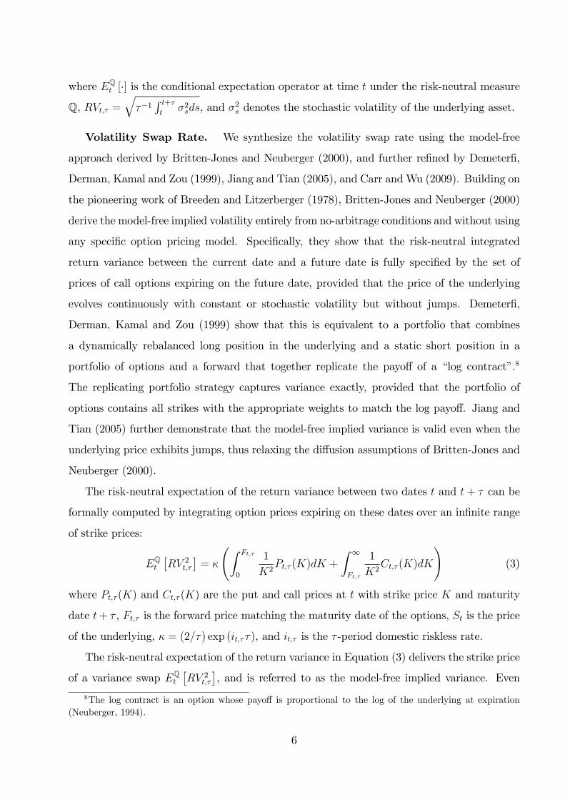
We provide a graphical illustration of the differences in the performance of carry, mo-

mentum and the VRP-strategy in Figure 1, which plots the one-year rolling Sharpe ratio for

the three strategies. The graphs make visually clear the marked difference in the evolution

of risk-adjusted returns of the VRP-based strategy relative to carry and momentum. It is

also clear that the average Sharpe ratio of the VRP-sorted strategy is not driven entirely or

primarily by a particular episode or sample period as the Sharpe ratio has been relatively

stable over the sample, and appears to be no more volatile than the Sharpe ratio of carry

and momentum. Finally, in Figure 2 we report cumulative returns over time for the three

strategies, for both the sample of developed countries and the full sample. Of particular

interest is the decomposition of the cumulative excess return into its two constituents: the

exchange rate component (FX) and the interest rate gain component (yield). Both carry and

momentum strategies have a positive yield component, although in the case of the carry trade

the yield component is the sole positive driver of the carry return because the cumulative FX

return component is negative. For momentum, most of the excess return is driven by spot pre-

dictability so the cumulative yield component has a positive but relatively minor contribution

to momentum returns. The VRP-based portfolio returns are very different in that they are

made up of a negative yield component (for both sample of countries considered) and there-

fore the component due to spot return predictability is in fact larger than the full portfolio

return from the VRP-strategy. In short, the VRP-strategy is the only strategy for which the

interest rate differential across countries detracts from the full portfolio return, which makes

it non-controversial that the VRP contains predictive information only about spot exchange

rate fluctuations, not interest rates.

Taken together, the results from the previous analysis and from the double sorting exercise

suggest that, while the carry trade strategy is — taken in isolation — the best performing

strategy in terms of excess returns and delivers the highest Sharpe ratio, the VRP strategy

has much stronger predictive power than either carry or momentum for exchange rate returns

and the predictive information content is largely independent of carry and momentum. This

18

means that a currency manager would benefit greatly from adding the VRP strategy to carry

and momentum to enhance risk-adjusted returns, and also that a spot trader interested in

forecasting exchange rate fluctuations (as opposed to excess returns) would value the VRP

strategy more than carry and momentum.

4.3 Pricing the Returns from VRP-sorted portfolios

In this section we carry out some cross-sectional asset pricing tests to determine whether the

returns from the VRP-based strategy can be understood as compensation for systematic risk.

The results rely on a standard stochastic discount factor (SDF) approach (Cochrane, 2005),

and we focus on a set of risk factors in our investigation that are motivated by the existing

currency asset pricing literature.

We start by briefly reviewing the methods employed, and denote excess returns of portfolio

i in period t + 1 by RX it+1. The usual no-arbitrage relation applies so that risk-adjusted

currency excess returns have a zero price and satisfy the basic Euler equation:

E[Mt+1RXit+1] = 0 (9)

with a linear SDFMt = 1−b′(Ht−µ) andH denoting a vector of risk factors. b is the vector of

SDF parameters and µ denotes factor means. This specification implies a beta pricing model

where expected excess returns depend on factor risk prices λ and risk quantities βi, which are

the regression betas of portfolio excess returns on the risk factors:

E[RX i

]= λ′βi (10)

for each portfolio i (see e.g., Cochrane, 2005). The relationship between the factor risk prices

in Equation (10) and the SDF parameters in Equation (9) is given by λ = ΣHb such that factor

risk prices, as in the traditional Fama-MacBeth (FMB) approach, can be easily obtained via

the SDF approach as well. We estimate parameters of Equation (9) via the generalized method

of moments (GMM).21

21Estimation is based on a pre-specified weighting matrix and we focus on unconditional moments (i.e. wedo not use instruments other than a constant vector of ones) since our interest lies in the performance of themodel to explain the cross-section of expected currency excess returns per se (see Cochrane, 2005; Burnside,2011).

19

In our asset pricing tests we consider a two-factor linear model that comprises DOL and

one more risk factor (RF ), which is one of HMLFX , V OLFX , ILLIQFX , and ILLIQV P ,

which we define below. DOL denotes the average return from borrowing in the US money

market and equally investing in foreign money markets. HMLFX is a long-short strategy that

buys (sells) the top 20% of all currencies currencies with the highest (lowest) interest rate

differential relative to the US dollar (see Lustig, Roussanov and Verdelhan, 2011). V OLFX

denotes a global FX volatility risk factor constructed as the innovations to global FX volatility.

ILLIQFX is a global FX illiquidity factor constructed as the global bid-ask spread of spot

exchange rates. V OLFX and ILLIQFX are constructed as in Menkhoff, Sarno, Schmeling and

Schrimpf (2012a). ILLIQV P is a global illiquidity factor for FX options constructed exactly

like ILLIQFX except that we use the bid-ask spread of the at-the-money implied volatilities

rather than the bid-ask spread of currencies.

In Table 6 we report GMM estimates of b and implied λs as well as cross-sectional R2s and

the Hansen-Jagannathan (HJ) distance measure (Hansen and Jagannathan, 1997). Standard

errors are based on Newey and West (1987) with optimal lag length selection according to

Andrews (1991).22 In assessing our results, we are aware of the statistical problems plaguing

standard asset pricing tests, recently emphasized by Lewellen, Nagel and Shanken (2010):

specifically, asset-pricing tests are often highly misleading in the sense that they can indicate

illusory strong explanatory power in terms of high cross-sectional R2 and small pricing errors

when in fact a risk factor has no or weak pricing power. Given the relatively small cross-

section of currencies and time span of our sample, these problems can be severe in our tests.

Hence, in interpreting our results, we only consider the cross-sectional R2 and HJ tests on

the pricing errors if we can confidently detect a statistically significant risk factor, i.e., if the

GMM estimates clearly point to a statistically significant market price of risk. Starting from

Panel A of Table 6, we can see clearly how none of the risk factors considered enters the

22Besides the GMM tests, we employ the traditional FMB two-pass OLS methodology to estimate portfoliobetas and factor risk prices. Note that we do not include a constant in the second stage of the FMB regressions,i.e. we do not allow a common over- or under-pricing in the cross-section of returns. We point out, however,that our results are virtually identical when we replace the DOL factor with a constant in the second stageregressions. Since DOL has basically no cross-sectional relation to the carry trade portfolios’returns, it servesthe same purpose as a constant that allows for a common mispricing. Also see Lustig and Verdelhan (2007)and Burnside (2011) on the issue of whether to include a constant or not. The FMB results are qualitativelyand in most cases also quantitatively identical to the one-step GMM results reported in Table 6, and hencenot reported to conserve space.

20

SDF with a statistically significant risk price λ, and this is the case for both the developed

countries and the full sample. The best performing SDF includes DOL and ILLIQV P which

generates some highly respectable cross-sectional R2 (0.57 and 0.80) but the market price of

risk is marginally insignificantly different from zero. The HJ test delivers large p-values for

the null of zero pricing errors in all cases but we attach no information to this result given

the lack of clear statistical significance of the market price of risk.

Panel B of Table 6 reports asset pricing tests, carried out using the same methods and

risk factors as for Panel A, where we attempt to price only the exchange rate component

of the returns from the VRP-based strategy. The results are equally disappointing in that

all risk factors included in the various SDF specifications are statistically insignificant except

ILLIQV P , which enters significantly and an intuitively clear positive sign —higher illiquidity

in the options market is associated with higher returns from the VRP strategy. However, even

this result is not particularly convincing, as the vector of SDF parameters b is insignificantly

different from zero.

Overall, the asset pricing tests in this section reveal that it is not possible to understand the

returns from the VRP strategy as compensation for risk using the carry risk factor and global

measures of volatility risk and illiquidity in the FX market of the kind used in the literature.

While this result is somewhat disappointing, it is also consistent with our earlier results

that indicate that the VRP portfolio returns are very different from carry and momentum

returns, and hence their source is likely to stem from a different mechanism rather than as a

compensation for canonical sources of systematic risk.23 Therefore, we now turn to examine

an alternative mechanism.

4.4 Explaining the Performance of the VRP strategy

A potential explanation for the predictive power of the VRP is that it arises from the inter-

action between natural hedgers of FX risk and speculators. The explanation has additional

testable implications which we test in Table 7. The table presents coeffi cients from predictive

time-series regressions of the exchange rate component of the VRP-sorted portfolio returns

23In unreported results, we also carried out asset pricing tests where we use the three-factor Fama-Frenchmodel, and also its four-factor variant that also allows for equity momentum. These equity risk factors arealso unable to price the returns from the VRP strategy.

21

on a number of conditioning factors implied by our proposed mechanism. We report results

from the exchange rate component of the VRP returns since we are primarily interested in

understanding the predictive power of the VRP for spot exchange rates, but the results for

the VRP portfolio returns are, not surprisingly, qualitatively identical and quantitatively very

similar.

The first column in both panels shows the univariate regression of the exchange rate

component of the VRP portfolio returns on the lagged TED spread. At times when funding

liquidity is lower (i.e., times of high capital constraints on speculators), we should find that the

expected (exchange rate) return from the VRP strategy should increase, and Table 7 provides

strong confirmation for this for developed countries. While the sign of the coeffi cient on TED

is positive for the full sample, it is not statistically significant. In our view, this could be

because the TED spread is possibly less useful as a proxy for funding liquidity constraints for

emerging markets. The second column shows that when changes in VIX are positive, which we

use as a proxy to capture increases in the risk aversion of natural hedgers, the VRP strategy FX

return increases, again consistent with the explanation. Again, this result is only significant

for the sample of developed countries. The third column interacts TED with changes in VIX,

and finds strong statistically significant predictive power of this interaction for the FX returns

on our strategy in both developed and emerging countries.

The next two columns use data from CFTC’s Commitments of Traders reports, and create

measures of hedging demand for the carry trade, a favoured strategy of speculators. The

measure we consider is the net short position in Australian dollar futures plus the net long

position in the Japanese yen, normalized by total positions. The idea of this measure is that

it should capture the risk appetite of speculators —when the measure is high, it suggests that

speculators are averse to carry risk, in the sense that they are reluctant to take positions in

high interest rate currencies like the Australian dollar, and more inclined to go long futures

of safe haven currencies like the yen. We also substitute the Swiss franc for the yen and use

this alternative construction as a robustness check in the fifth column of each panel. Table 7

shows that, as predicted, when speculators’risk appetite is diminished, the expected returns

to the VRP-sorted strategy increase. This is true for both measures that we consider.

The final columns in the two panels of the table add in measures of capital flows into

hedge funds, constructed as the change in assets under management less accrued returns,

22

normalized by lagged assets under management of the combined universe of hedge funds in

the TASS, HFR, CISDM, Barclay Hedge and Morningstar databases (with roughly $2 trillion

under management as of end 2012). When capital flows into hedge funds are high, signifying

that they experience fewer constraints on their ability to engage in arbitrage transactions and

provide insurance, we find that the returns for our VRP-sorted portfolio are lower and vice

versa.

The final three rows of Table 7 add in several of the variables described above together to

test their joint explanatory power, and individual contributions to the proposed explanation of

our results that relies on the interaction between hedgers and speculators in currency markets.

We include TED, changes in VIX and the interaction separately to avoid potential collinearity

in the regressions as these variables are highly correlated with one another. More generally,

it is clear that the variables used in the univariate regressions are likely to contain a substan-

tial common component. We find that all the variables retain their signs and are generally

statistically significant in these predictive regressions, offering support to the explanation of

our results.

Finally, we examine post-formation portfolio returns. Under our proposed explanation

for the spot predictability in the VRP, this predictability cannot be very long-lived. Recall

the scenario where speculators face a shock that reduces their available arbitrage capital and

limits their ability to provide cheap volatility insurance. Ned demand for volatility insurance

increases, making hedging more expensive, as reflected in a lower VRP for currencies. Given

the high cost of volatility insurance, natural hedgers scale back on the amount of spot currency

they are willing to hold, predictably depressing spot prices and leading to relatively low returns

on the spot currency position. When capital constraints loosen, however, we should see the

opposite behavior, i.e., a higher VRP and relatively higher returns on the spot currency

position. This implies — as a testable implication — reversal in post-formation cumulative

returns, which is exactly what we find. In Figure 3, we plot cumulative post-formation excess

returns (left) and exchange rate returns (right) over periods of 1, 2, . . . , 20 months for the

VRP-sorted portfolios, for both samples of countries examined. Specifically we plot returns

net of the exposure to carry trade risk, i.e., we use the residuals from a regression of portfolio

returns or exchange rate returns on HMLFX , so that the returns can be considered as alphas

23

over and above carry trade returns.24 Returns in the post-formation period are overlapping

since we form new portfolios each month but track these portfolios for 20 months. Starting

from excess returns, there is a clear pattern of increasing returns that peaks after 3 months

for the developed countries sample and 4 months for the full sample, and a subsequent period

of declining excess returns. Looking at spot exchange rate returns (the FX component of the

strategy returns), the peak in cumulative post-formation exchange rate return actually occurs

around 4 months for the developed sample and 5-6 months for the full sample. Thus, on the

face of it, this evidence looks consistent with the reversal implied by our proposed explanation

of the economic source of VRP predictive power.

Overall, taken together, the empirical results in this section lend some support to our

proposed explanation for the predictability of spot exchange rates arising from the VRP,

and the mechanism considered here is consistent with the growing theoretical and empirical

literature that highlights the role of limits to arbitrage and the interaction between hedgers

and speculators in asset markets.

5 Conclusions

We show that the currency volatility risk premium (VRP) has substantial predictive power for

the cross-section of currency returns. Sorting currencies on the VRP generates economically

significant returns in a standard multi-currency portfolio setting. This predictive power is

specifically related to spot exchange rate returns, not interest rate differentials, and the spot

rate predictability is much stronger than that observed from carry and currency momentum

strategies. Specifically, currencies for which volatility insurance is relatively cheap tend to

predictably appreciate, while currencies for which volatility hedging is relatively expensive

tend to predictably depreciate. We also find that the returns from our VRP-sorted strategy

are largely uncorrelated with carry and momentum strategies, thus providing a substantial

diversification gain to investors. We confirm that double sorting currency portfolios by both

the VRP and either carry or momentum does not affect the predictive power of the VRP.

Finally, standard risk factors cannot price satisfactorily the returns from portfolios sorted on

24Using raw portfolio returns or their exchange rate component produces a very similar pattern for the fullsample, and a virtually identical pattern for the developed sample, as expected given that we know alreadyfrom previous analyses that HMLFX has almost no pricing power for the VRP-sorted returns.

24

the VRP, corroborating the notion that this strategy delivers a source of predictable returns

that cannot easily be replicated using extant trading strategies.

We provide some evidence that the exchange rate predictability embedded in the VRP can

be rationalized in terms of the time-variation of limits to arbitrage capital and the incentives of

hedgers and speculators in financial markets. Specifically, the returns from the VRP strategy

appear to be higher at times when funding liquidity is lower, risk aversion is higher, and

there is increasing demand for hedging high-risk currency positions. This seems consistent

with the notion that risk-averse natural “hedgers”of currencies such as multinational firms,

or financial institutions that inherit currency positions from their clients, are more willing to

hold currencies for which volatility insurance is relatively inexpensive. Such institutions will

also be more likely to avoid holding, or be more likely to sell, positions in currencies with

expensive volatility protection. The pattern of exchange rate predictability stemming from

the VRP appears to be empirically consistent with this simple mechanism.

Overall, the results in this paper provide new insights into the predictability of the cross-

section of exchange rate returns and the linkages between the cost of volatility protection and

the returns from underlying currencies.

25

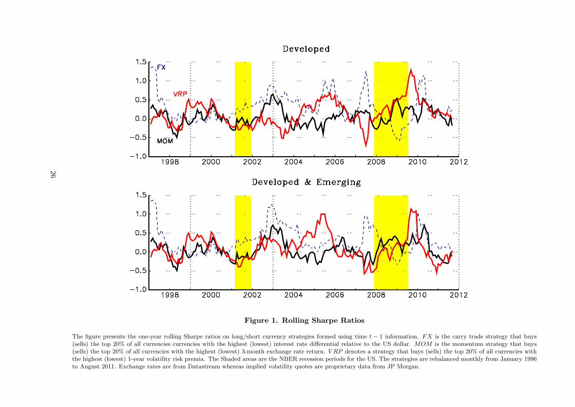
Figure 1. Rolling Sharpe Ratios

The figure presents the one-year rolling Sharpe ratios on long/short currency strategies formed using time t − 1 information. FX is the carry trade strategy that buys(sells) the top 20% of all currencies currencies with the highest (lowest) interest rate differential relative to the US dollar. MOM is the momentum strategy that buys(sells) the top 20% of all currencies with the highest (lowest) 3-month exchange rate return. V RP denotes a strategy that buys (sells) the top 20% of all currencies withthe highest (lowest) 1-year volatility risk premia. The Shaded areas are the NBER recession periods for the US. The strategies are rebalanced monthly from January 1996to August 2011. Exchange rates are from Datastream whereas implied volatility quotes are proprietary data from JP Morgan.

26

Figure 2. Currency Strategies and Payoffs

The figure presents the cumulative payoffs of long/short currency strategies formed using time t− 1 information. FX is the carry trade strategy that buys (sells) the top20% of all currencies currencies with the highest (lowest) interest rate differential relative to the US dollar. MOM is the momentum strategy that buys (sells) the top20% of all currencies with the highest (lowest) 3-month exchange rate return. V RP denotes a strategy that buys (sells) the top 20% of all currencies with the highest(lowest) 1-year volatility risk premia. The strategies are rebalanced monthly from January 1996 to August 2011. Exchange rates are from Datastream whereas impliedvolatility quotes are proprietary data from JP Morgan.

27

Figure 3. Long-horizon Returns

This figure presents cumulative average returns to the long/short V RP strategy after portfolio formation. V RP buys (sells) the top 20% of all currencies with the highest(lowest) 1-year volatility risk premia known at time t−1. Post-formation returns are constructed for 1, 2, . . . , 20 months following the formation period. This is equivalentto building new portfolios every month and recording them for the subsequent 20 months (using overlapping horizons). We cumulate risk-adjusted (with respect to thecarry trade strategy) currency excess returns and exchange rate returns. The strategies are rebalanced monthly from January 1996 to August 2011. Exchange rates arefrom Datastream whereas implied volatility quotes are proprietary data from JP Morgan.

28

Table 1. Descriptive Statistics of Volatility Risk Premia

This table presents summary statistics for the annualized average realized volatility RVt,τ (Panel A), synthetic volatility swap rate SWt,τ (Panel B),and volatility risk premium V RPt,τ = RVt,τ −SWt,τ (Panel C ) where τ , the maturity of the volatility swap, is equal to 1-year. RVt,τ is computed at timet using daily exchange rate returns between times t− τ and t. SWt,τ is constructed at time t using τ -period implied volatilities across 5 different deltas asin Jiang and Tian (2005). The volatility risk premium V RPt,τ is constructed as the difference between RVt,τ and SWt,τ . Qj refers to the jth percentile.ACτ indicates the τ th-order autocorrelation coeffi cient. The sample period comprises daily data from January 1996 to August 2011. Exchange rates arefrom Datastream whereas implied volatility quotes are proprietary data from JP Morgan.

RVt,τ × 100 SWt,τ × 100 V RPt,τ × 100 RVt,τ × 100 SWt,τ × 100 V RPt,τ × 100

Developed Developed & EmergingMean 10.68 11.31 −0.62 10.82 11.74 −0.92

Sdev 2.88 2.75 1.58 3.10 3.22 1.78

Skew 1.85 1.42 0.54 2.12 2.07 −0.31

Kurt 6.86 5.29 5.97 7.85 8.06 7.88

Q5 7.15 7.77 −3.06 7.23 8.36 −3.67

Q95 18.40 16.76 1.65 19.43 17.86 1.57

ACτ 0.33 0.53 −0.19 0.27 0.46 −0.17

29

Table 2. Descriptive Statistics of Currency Strategies

This table presents descriptive statistics of long/short currency strategies formed using time t − 1 information. FX is the carry trade strategy thatbuys (sells) the top 20% of all currencies with the highest (lowest) interest rate differential relative to the US dollar. MOM is the momentum strategythat buys (sells) the top 20% of all currencies with the highest (lowest) lagged 3-month exchange rate return. V RP denotes a strategy that buys (sells)the top 20% of all currencies with the highest (lowest) 1-year volatility risk premia. The table also reports the first order autocorrelation coeffi cient (AC1),the annualized Sharpe ratio (SR), the Sortino ratio (SO), the maximum drawdown (MDD), and the frequency of portfolio switches for the long (FreqL)and the short (FreqS) position. Newey and West (1987) standard errors with Andrews (1991) optimal lag selection are reported in parenthesis. Panel Adisplays the overall currency excess return whereas Panel B reports only the exchange rate component. Returns are expressed in percentage per annum.The strategies are rebalanced monthly from January 1996 to August 2011. Exchange rates are from Datastream whereas implied volatility quotes areproprietary data from JP Morgan.

Panel A: Currency Excess Returns

FX MOM VRP FX MOM VRP

Developed Developed & EmergingMean 6.49 2.58 4.03 7.42 2.22 2.34

Sdev 10.66 9.55 8.33 9.97 8.30 8.18

Skew −0.92 0.35 0.28 −0.92 −0.03 0.12

Kurt 5.65 3.86 3.47 4.53 2.95 3.26

SR 0.61 0.27 0.48 0.74 0.27 0.29

(0.089) (0.068) (0.072) (0.080) (0.069) (0.075)

SO 0.72 0.50 0.87 0.94 0.47 0.49

MDD −0.37 −0.16 −0.18 −0.21 −0.13 −0.18

AC1 0.09 0.01 0.04 0.01 −0.09 0.05

FreqL 0.13 0.48 0.24 0.15 0.49 0.26

FreqS 0.07 0.43 0.32 0.16 0.46 0.27

Panel B: Exchange Rate Returns

Mean 0.34 2.03 4.40 −0.65 1.45 3.72

Sdev 10.66 9.57 8.35 9.99 8.16 8.17

Skew −0.93 0.42 0.28 −1.05 −0.02 0.12

Kurt 5.82 4.17 3.61 4.84 3.13 3.50

SR 0.03 0.21 0.53 −0.07 0.18 0.46

(0.079) (0.068) (0.072) (0.072) (0.067) (0.075)

SO 0.04 0.40 0.93 −0.08 0.30 0.75

MDD −0.43 −0.20 −0.19 −0.35 −0.15 −0.18

AC1 0.11 0.01 0.04 0.03 −0.12 0.04

FreqL 0.13 0.48 0.24 0.15 0.49 0.26

FreqS 0.07 0.43 0.32 0.16 0.46 0.27

30

Table 3. Sample Correlations of Currency Strategies

This table presents the sample correlations of long/short currency strategies formed using time t− 1 information. FX is the carry trade strategy thatbuys (sells) the top 20% of all currencies currencies with the highest (lowest) interest rate differential relative to the US dollar. MOM is the momentumstrategy that buys (sells) the top 20% of all currencies with the highest (lowest) 3-month exchange rate return. V RP denotes a strategy that buys (sells)the top 20% of all currencies with the highest (lowest) 1-year volatility risk premia. Panel A displays the overall currency excess return whereas Panel Breports only the exchange rate component. The strategies are rebalanced monthly from January 1996 to August 2011. Exchange rates are from Datastreamwhereas implied volatility quotes are proprietary data from JP Morgan.

Panel A: Currency Excess ReturnsFX MOM VRP FX MOM VRP

Developed Developed & EmergingFX 1.00 1.00MOM −0.17 1.00 −0.03 1.00V RP −0.18 0.09 1.00 −0.21 0.10 1.00

Panel B: Exchange Rate ReturnsFX 1.00 1.00MOM −0.17 1.00 −0.04 1.00V RP −0.19 0.10 1.00 −0.22 0.12 1.00

31

Table 4. Portfolios Sorted on Volatility Risk Premia

This table presents descriptive statistics of five currency portfolios sorted on the 1-year volatility risk premia V RP at time t − 1. The first (last)portfolio PL (PS) contains the top 20% of all currencies with the highest (lowest) volatility risk premia. DOL is the average of the currency portfolios.HML is a long-short strategy that buys PL and sells PS . The table also reports the first order autocorrelation coeffi cient (AC1), the annualized Sharperatio (SR), the Sortino ratio (SO), the maximum drawdown (MDD), and the frequency of portfolio switches (Freq). Newey and West (1987) standarderrors with Andrews (1991) optimal lag selection are reported in parenthesis. Panel A displays the overall currency excess return, whereas Panel B reportsonly the exchange rate component. Returns are expressed in percentage per annum. The strategies are rebalanced monthly from January 1996 to August2011. Exchange rates are from Datastream whereas implied volatility quotes are proprietary data from JP Morgan.

Panel A: Currency Excess Returns

PL P2 P3 P4 PS DOL HML PL P2 P3 P4 PS DOL HML

Developed Developed & EmergingMean 4.70 2.24 1.04 1.78 0.67 2.08 4.03 3.59 1.93 1.34 1.40 1.26 1.90 2.34

Sdev 9.08 9.27 9.76 10.07 9.72 8.14 8.33 9.32 8.68 8.89 10.44 8.81 8.07 8.18

Skew −0.05 0.19 0.09 −0.17 −0.26 0.00 0.28 −0.09 0.05 −0.21 −0.29 −0.39 −0.25 0.12

Kurt 3.13 5.14 5.80 3.85 3.82 3.95 3.47 3.09 4.79 3.85 4.16 3.73 4.37 3.26

SR 0.52 0.24 0.11 0.18 0.07 0.26 0.48 0.39 0.22 0.15 0.13 0.14 0.24 0.29

(0.078) (0.084) (0.077) (0.081) (0.073) (0.073) (0.073) (0.074) (0.085) (0.079) (0.078) (0.075) (0.086) (0.072)

SO 0.85 0.39 0.16 0.27 0.10 0.41 0.87 0.62 0.35 0.22 0.19 0.20 0.34 0.49

MDD −0.27 −0.36 −0.43 −0.35 −0.32 −0.31 −0.18 −0.27 −0.37 −0.42 −0.35 −0.30 −0.31 −0.18

AC1 0.10 0.04 0.13 0.15 0.01 0.13 0.04 0.10 0.14 0.15 0.13 0.11 0.16 0.05

Freq 0.24 0.44 0.52 0.48 0.32 0.24 0.32 0.26 0.43 0.53 0.48 0.27 0.26 0.27

Panel B: Exchange Rate Returns

Mean 4.93 2.06 1.26 1.60 0.52 2.07 4.40 3.51 1.62 1.37 0.82 −0.21 1.42 3.72

Sdev 9.05 9.24 9.63 9.96 9.64 8.05 8.35 9.26 8.62 8.74 10.31 8.75 7.98 8.17

Skew −0.12 0.15 0.06 −0.18 −0.26 −0.02 0.28 −0.18 0.00 −0.26 −0.31 −0.47 −0.33 0.12

Kurt 3.17 5.24 5.88 4.06 3.83 3.99 3.61 3.07 4.80 4.02 4.36 3.94 4.56 3.50

SR 0.54 0.22 0.13 0.16 0.05 0.26 0.53 0.38 0.19 0.16 0.08 −0.02 0.18 0.46

(0.078) (0.082) (0.078) (0.081) (0.073) (0.078) (0.072) (0.074) (0.084) (0.081) (0.074) (0.075) (0.084) (0.075)

SO 0.87 0.35 0.20 0.25 0.08 0.41 0.93 0.59 0.29 0.23 0.11 −0.03 0.25 0.75

MDD −0.26 −0.34 −0.38 −0.31 −0.29 −0.27 −0.19 −0.26 −0.34 −0.36 −0.32 −0.30 −0.27 −0.18

AC1 0.10 0.03 0.11 0.13 −0.01 0.12 0.04 0.10 0.13 0.13 0.10 0.10 0.15 0.04

Freq 0.24 0.44 0.52 0.48 0.32 0.24 0.32 0.26 0.43 0.53 0.48 0.27 0.26 0.27

32

Table 5. Double-Sorted Currency Strategies

This table presents descriptive statistics of long/short currency strategies formed by double-sorting currencies into 4 groups using time t−1 information.Currencies are first sorted into 2 groups according to the 3-month exchange rate returns (or volatility risk premia) and then re-sorted using the interest ratedifferentials relative to the US dollar. MOM (V RP ) is the high-minus-low currency strategy on the 3-month exchange rate returns (the 1-year expectedvolatility premia) whereas FX is the high-minus-low currency strategy on the interest rate differentials relative to the US dollar. The table also reportsthe first order autocorrelation coeffi cient (AC1), the annualized Sharpe ratio (SR), the Sortino ratio (SO), the maximum drawdown (MDD), and thefrequency of portfolio switches for the long (FreqL) and the short (FreqS) position. Newey and West (1987) standard errors with Andrews (1991) optimallag selection are reported in parenthesis. Panel A displays the overall currency excess return whereas Panel B reports only the exchange rate component.Returns are expressed in percentage per annum. The strategies are rebalanced monthly from January 1996 to August 2011. Exchange rates are fromDatastream whereas implied volatility quotes are proprietary data from JP Morgan.

Panel A: Currency Excess Returns

=⇒ =⇒ =⇒ =⇒ =⇒ =⇒MOM FX V RP FX V RP MOM MOM FX V RP FX V RP MOM

Developed Developed & EmergingMean 1.43 3.28 2.38 3.34 2.02 1.64 1.03 3.33 1.08 4.27 0.84 2.12

Sdev 6.42 5.51 4.73 5.68 4.80 5.65 5.73 5.08 4.76 5.67 4.80 5.03

Skew 0.09 −0.59 −0.33 −0.69 −0.03 0.11 −0.37 −0.84 0.03 −1.00 0.20 −0.10

Kurt 4.54 5.09 3.42 4.15 3.29 3.66 3.87 4.17 3.78 4.63 3.79 4.34

SR 0.22 0.60 0.50 0.59 0.42 0.29 0.18 0.66 0.23 0.75 0.18 0.42

(0.073) (0.078) (0.067) (0.082) (0.072) (0.071) (0.074) (0.074) (0.072) (0.085) (0.072) (0.070)

SO 0.33 0.77 0.77 0.78 0.70 0.50 0.25 0.84 0.37 0.99 0.30 0.64

MDD −0.16 −0.15 −0.13 −0.18 −0.14 −0.11 −0.16 −0.10 −0.15 −0.17 −0.15 −0.09

AC1 0.04 −0.05 −0.07 0.03 0.05 0.05 0.07 −0.06 −0.02 0.14 0.03 −0.01

FreqL 0.36 0.36 0.27 0.27 0.47 0.47 0.38 0.38 0.27 0.27 0.43 0.43

FreqS 0.38 0.38 0.31 0.31 0.47 0.47 0.38 0.38 0.29 0.29 0.42 0.42

Panel B: Exchange Rate Returns

Mean 0.22 0.32 1.97 0.38 2.08 1.19 0.17 −0.57 1.52 0.32 1.54 1.57

Sdev 6.42 5.52 4.74 5.71 4.83 5.65 5.67 5.11 4.81 5.73 4.85 5.01

Skew 0.18 −0.58 −0.40 −0.72 −0.08 0.17 −0.31 −0.92 −0.01 −1.10 0.19 −0.09

Kurt 4.84 5.16 3.42 4.24 3.33 3.95 3.92 4.33 3.90 4.98 3.95 4.64

SR 0.03 0.06 0.42 0.07 0.43 0.21 0.03 −0.11 0.32 0.06 0.32 0.31

(0.073) (0.076) (0.067) (0.080) (0.072) (0.073) (0.073) (0.058) (0.072) (0.086) (0.072) (0.073)

SO 0.05 0.07 0.61 0.09 0.71 0.35 0.04 −0.14 0.51 0.07 0.55 0.47

MDD −0.25 −0.20 −0.15 −0.21 −0.14 −0.14 −0.23 −0.19 −0.15 −0.20 −0.15 −0.11

AC1 0.03 −0.04 −0.07 0.04 0.05 0.05 0.05 −0.04 −0.01 0.16 0.03 −0.02

FreqL 0.36 0.36 0.27 0.27 0.56 0.56 0.38 0.38 0.27 0.27 0.43 0.43

FreqS 0.38 0.38 0.31 0.31 0.58 0.58 0.38 0.38 0.29 0.29 0.42 0.42

33

Table 6. Asset Pricing Tests

This table reports asset pricing results for a linear factor model that includes DOL and RF as risk factors. Our risk factors includes HMLFX ,V OLFX , ILLIQFX , and ILLIQV P . The test assets are currency excess returns (Panel A) and exchange rate returns (Panel B) to five portfolios sortedon the 1-year volatility risk premia available at time t− 1. DOL denotes the average return from borrowing in the US money market and equally investingin foreign money markets. HMLFX is a long-short strategy that buys (sells) the top 20% of all currencies currencies with the highest (lowest) interestrate differential relative to the US dollar. V OLFX denotes the global FX volatility risk factor constructed as the innovations to the average exchange ratevolatility across currencies. ILLIQFX is the illiquidity risk factor constructed using the average bid-ask spreads across our spot exchange rates. ILLIQV Pis the illiquidity risk factor constructed using the average bid-ask spreads of the at-the-money implied volatilities. The table reports one-stage GMMestimates of the factor loadings b, and the market price of risk λ. The χ2 and the Hansen-Jagannathan distance are test statistics for the null hypothesisthat all pricing errors are jointly zero. Newey and West (1987) standard errors with Andrews (1991) optimal lag selection are reported in parenthesis. Thep-values are reported in brackets. Returns are expressed in percentage per annum. The portfolios are rebalanced monthly from January 1996 to August2011. Exchange rates are from Datastream whereas implied volatility quotes are proprietary data from JP Morgan.

Panel A: Currency Excess ReturnsRF bDOL bRF λDOL λRF R2 RMSE χ2 HJ bDOL bRF λDOL λRF R2 RMSE χ2 HJ

Developed Developed & EmergingHMLFX 0.42 −0.47 0.02 −0.05 −0.07 3.29 4.35 0.16 0.24 0.01 0.02 0.01 −0.14 2.09 1.93 0.11

(0.36) (0.55) (0.02) (0.07) [0.23] [0.20] (0.35) (0.51) (0.02) (0.06) [0.59] [0.59]

V OLFX 0.52 0.36 0.02 0.57 0.26 2.74 3.02 0.13 0.48 0.16 0.02 0.29 −0.07 2.04 2.31 0.11

(0.32) (0.23) (0.02) (0.37) [0.39] [0.44] (0.72) (0.43) (0.02) (0.78) [0.51] [0.55]

ILLIQFX 0.32 0.40 0.02 0.02 0.03 2.59 3.81 0.13 0.74 4.50 0.02 0.21 0.26 2.62 3.58 0.15

(0.59) (2.62) (0.02) (0.13) [0.28] [0.39] (0.66) (5.87) (0.02) (0.16) [0.31] [0.53]

ILLIQV P 0.83 14.78 0.02 0.10 0.57 2.10 1.23 0.11 0.18 5.63 0.02 0.10 0.80 0.87 0.32 0.05

(0.71) (11.72) (0.02) (0.06) [0.75] [0.87] (0.32) (5.33) (0.02) (0.07) [0.96] [0.96]

Panel B: Exchange Rate ReturnsHMLFX 0.43 −0.50 0.02 −0.06 −0.05 3.46 5.23 0.17 0.30 −0.44 0.01 −0.05 0.13 2.54 3.12 0.13

(0.36) (0.52) (0.02) (0.07) [0.16] [0.14] (0.34) (0.47) (0.02) (0.05) [0.37] [0.37]

V OLFX 0.58 0.42 0.02 0.65 0.35 2.74 2.74 0.13 0.94 0.48 0.02 0.94 0.26 2.34 2.47 0.12

(0.33) (0.25) (0.02) (0.38) [0.43] [0.47] (0.87) (0.49) (0.02) (0.76) [0.48] [0.55]

ILLIQFX 0.37 0.77 0.02 0.04 0.05 2.54 3.87 0.13 0.74 5.08 0.01 0.24 0.39 2.28 2.07 0.13

(0.67) (3.31) (0.02) (0.15) [0.28] [0.37] (0.61) (5.42) (0.02) (0.14) [0.56] [0.65]

ILLIQV P 0.77 14.77 0.02 0.10 0.53 2.33 1.61 0.12 0.14 6.42 0.02 0.13 0.77 1.32 0.71 0.08

(0.66) (11.36) (0.02) (0.05) [0.66] [0.83] (0.36) (5.52) (0.02) (0.07) [0.87] [0.90]

34

Table 7. Risk Factors: Liquidity and Hedging

This table presents least squares estimates of predictive regressions. The dependent variable is the monthly exchange rate component of the V RPstrategy at time t. This strategy is long/short portfolio that buys (sells) the top 20% of all currencies with the highest (lowest) 1-year expected volatilitypremia at time t − 1. The predictors include the TED spread, the V IX index, the hedgers net position on carry trade strategies, proxied as net shortfutures position on Australian dollar A$ and net long futures position on the Japanese Yen U (Swiss franc SFr), and the changes in the number ofspeculators measured as net flow of new funds to hedge funds, scaled by the lagged assets under management. Newey and West (1987) standard errors arereported in parenthesis. The superscripts a, b, and c indicate statistical significance at 10%, 5%, and 1%, respectively. Returns are expressed in percentageper annum. Exchange rates are from Datastream, implied volatility quotes are from JP Morgan, hedging positions are from the US Commodity FuturesTrading Commission (CFTC), hedge fund flows are from Patton and Ramadorai (2013), whereas all other data are from Bloomberg.

TED× Hedging Position Hedge Fund TED× Hedging Position Hedge Fund

α TED ∆V IX ∆V IX A$/¥ A$/SFr F lows R2(%) α TED ∆V IX ∆V IX A$/¥ A$/SFr F lows R

2(%)

Developed Developed & Emerging−0.301 1.326b 3.0 0.043 0.530 0.1(0.278) (0.570) (0.286) (0.548)

0.350b 0.004a 1.4 0.297a 0.003 0.7(0.172) (0.002) (0.171) (0.002)

0.258 0.007c 4.7 0.234 0.005c 2.1(0.160) (0.001) (0.166) (0.002)

0.385b 0.130c 1.5 0.327a 0.119c 1.2(0.182) (0.016) (0.176) (0.017)

0.388b 0.130c 1.5 0.330a 0.121c 1.3(0.182) (0.022) (0.177) (0.022)

0.458b −0.125a 2.4 0.379a −0.095a 1.2(0.204) (0.065) (0.193) (0.061)

−0.074 1.023a 0.119c −0.079 4.8 0.268 0.229 0.110c −0.079 1.8(0.335) (0.609) (0.015) (0.061) (0.330) (0.57) (0.018) (0.062)

0.442b 0.003 0.118c −0.098a 4.0 0.369b 0.002 0.110c −0.073 2.3(0.191) (0.002) (0.015) (0.058) (0.186) (0.002) (0.017) (0.057)

0.348a 0.006c 0.118c −0.080 6.6 0.306a 0.004c 0.110c −0.062 3.5(0.182) (0.001) (0.015) (0.053) (0.185) (0.002) (0.017) (0.056)

35

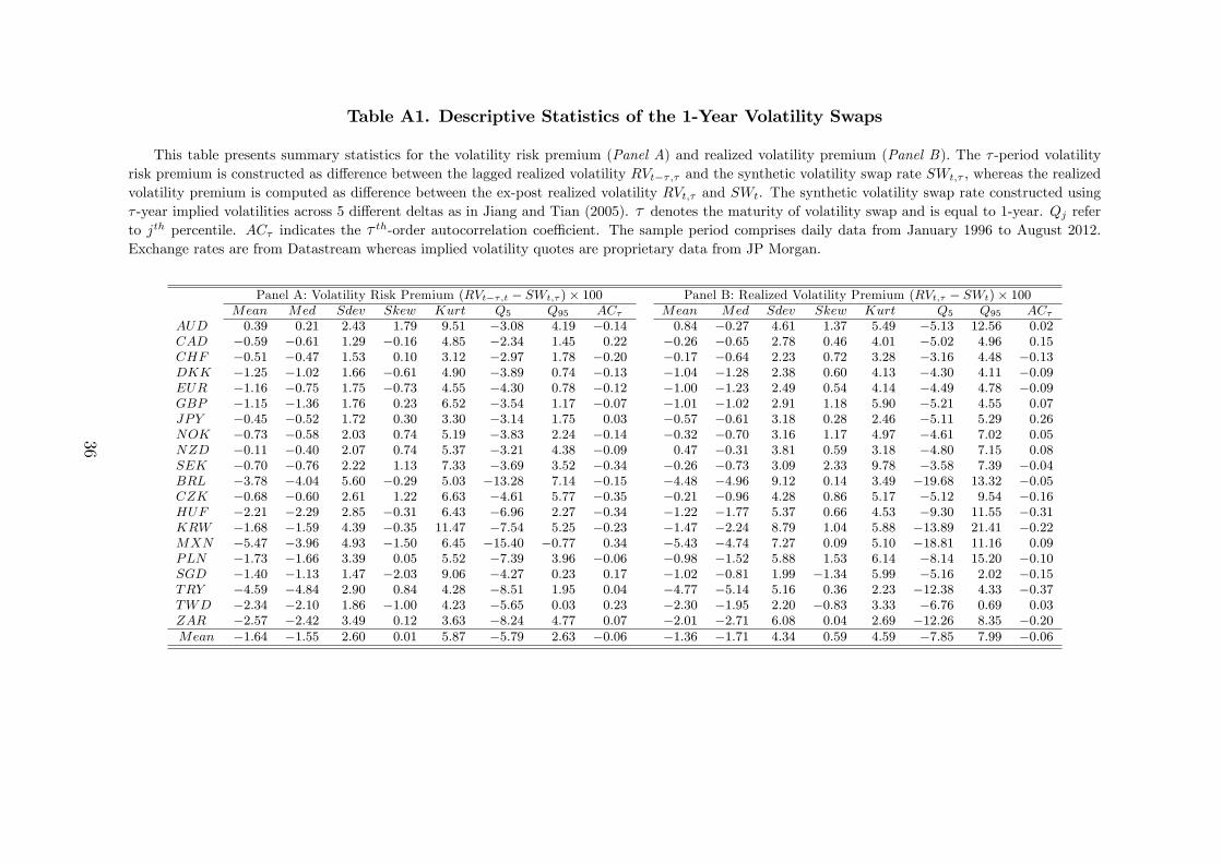
Table A1. Descriptive Statistics of the 1-Year Volatility Swaps

This table presents summary statistics for the volatility risk premium (Panel A) and realized volatility premium (Panel B). The τ -period volatilityrisk premium is constructed as difference between the lagged realized volatility RVt−τ,τ and the synthetic volatility swap rate SWt,τ , whereas the realizedvolatility premium is computed as difference between the ex-post realized volatility RVt,τ and SWt. The synthetic volatility swap rate constructed usingτ -year implied volatilities across 5 different deltas as in Jiang and Tian (2005). τ denotes the maturity of volatility swap and is equal to 1-year. Qj referto jth percentile. ACτ indicates the τ th-order autocorrelation coeffi cient. The sample period comprises daily data from January 1996 to August 2012.Exchange rates are from Datastream whereas implied volatility quotes are proprietary data from JP Morgan.

Panel A: Volatility Risk Premium (RVt−τ,t − SWt,τ )× 100 Panel B: Realized Volatility Premium (RVt,τ − SWt)× 100Mean Med Sdev Skew Kurt Q5 Q95 ACτ Mean Med Sdev Skew Kurt Q5 Q95 ACτ

AUD 0.39 0.21 2.43 1.79 9.51 −3.08 4.19 −0.14 0.84 −0.27 4.61 1.37 5.49 −5.13 12.56 0.02CAD −0.59 −0.61 1.29 −0.16 4.85 −2.34 1.45 0.22 −0.26 −0.65 2.78 0.46 4.01 −5.02 4.96 0.15CHF −0.51 −0.47 1.53 0.10 3.12 −2.97 1.78 −0.20 −0.17 −0.64 2.23 0.72 3.28 −3.16 4.48 −0.13DKK −1.25 −1.02 1.66 −0.61 4.90 −3.89 0.74 −0.13 −1.04 −1.28 2.38 0.60 4.13 −4.30 4.11 −0.09EUR −1.16 −0.75 1.75 −0.73 4.55 −4.30 0.78 −0.12 −1.00 −1.23 2.49 0.54 4.14 −4.49 4.78 −0.09GBP −1.15 −1.36 1.76 0.23 6.52 −3.54 1.17 −0.07 −1.01 −1.02 2.91 1.18 5.90 −5.21 4.55 0.07JPY −0.45 −0.52 1.72 0.30 3.30 −3.14 1.75 0.03 −0.57 −0.61 3.18 0.28 2.46 −5.11 5.29 0.26NOK −0.73 −0.58 2.03 0.74 5.19 −3.83 2.24 −0.14 −0.32 −0.70 3.16 1.17 4.97 −4.61 7.02 0.05NZD −0.11 −0.40 2.07 0.74 5.37 −3.21 4.38 −0.09 0.47 −0.31 3.81 0.59 3.18 −4.80 7.15 0.08SEK −0.70 −0.76 2.22 1.13 7.33 −3.69 3.52 −0.34 −0.26 −0.73 3.09 2.33 9.78 −3.58 7.39 −0.04BRL −3.78 −4.04 5.60 −0.29 5.03 −13.28 7.14 −0.15 −4.48 −4.96 9.12 0.14 3.49 −19.68 13.32 −0.05CZK −0.68 −0.60 2.61 1.22 6.63 −4.61 5.77 −0.35 −0.21 −0.96 4.28 0.86 5.17 −5.12 9.54 −0.16HUF −2.21 −2.29 2.85 −0.31 6.43 −6.96 2.27 −0.34 −1.22 −1.77 5.37 0.66 4.53 −9.30 11.55 −0.31KRW −1.68 −1.59 4.39 −0.35 11.47 −7.54 5.25 −0.23 −1.47 −2.24 8.79 1.04 5.88 −13.89 21.41 −0.22MXN −5.47 −3.96 4.93 −1.50 6.45 −15.40 −0.77 0.34 −5.43 −4.74 7.27 0.09 5.10 −18.81 11.16 0.09PLN −1.73 −1.66 3.39 0.05 5.52 −7.39 3.96 −0.06 −0.98 −1.52 5.88 1.53 6.14 −8.14 15.20 −0.10SGD −1.40 −1.13 1.47 −2.03 9.06 −4.27 0.23 0.17 −1.02 −0.81 1.99 −1.34 5.99 −5.16 2.02 −0.15TRY −4.59 −4.84 2.90 0.84 4.28 −8.51 1.95 0.04 −4.77 −5.14 5.16 0.36 2.23 −12.38 4.33 −0.37TWD −2.34 −2.10 1.86 −1.00 4.23 −5.65 0.03 0.23 −2.30 −1.95 2.20 −0.83 3.33 −6.76 0.69 0.03ZAR −2.57 −2.42 3.49 0.12 3.63 −8.24 4.77 0.07 −2.01 −2.71 6.08 0.04 2.69 −12.26 8.35 −0.20Mean −1.64 −1.55 2.60 0.01 5.87 −5.79 2.63 −0.06 −1.36 −1.71 4.34 0.59 4.59 −7.85 7.99 −0.06

36

Table A2. Asset Pricing Tests I

This table reports asset pricing results. The linear factor model includes the dollar (DOL) and the slope (HMLFX) risk factors. HMLFX is along-short strategy that buys (sells) the top 20% of all currencies currencies with the highest (lowest) interest rate differential relative to the US dollar.The test assets are currency excess returns (Panel A) and exchange rate returns (Panel B) to five portfolios sorted on the 1-year volatility risk premia(V RP ) available at time t− 1. The table reports GMM and Fama-MacBeth (FMB) estimates of the factor loadings b, the market price of risk λ, and leastsquares estimates of time series slopes β. The χ2 and the Hansen-Jagannathan distance are test statistics for the null hypothesis that all pricing errors arejointly zero. Newey and West (1987) standard errors with Andrews (1991) optimal lag selection and Shanken (1992) standard errors (sh) are reported inparenthesis. The p-values are reported in brackets. Excess returns are expressed in percentage per annum. The portfolios are rebalanced monthly fromJanuary 1996 to August 2011. Exchange rates are from Datastream whereas implied volatility quotes are proprietary data from JP Morgan.

Panel A: Currency Excess Returns

Factor PricesbDOL bHML λDOL λHML R2 RMSE χ2 HJ bDOL bHML λDOL λHML R2 RMSE χ2 HJ

Developed Developed & EmergingGMM1 0.42 −0.47 0.02 −0.05 −0.07 3.29 4.35 0.16 0.24 0.01 0.02 0.01 −0.14 2.09 1.93 0.11

(0.36) (0.55) (0.02) (0.07) [0.23] [0.20] (0.35) (0.51) (0.02) (0.06) [0.59] [0.59]

GMM2 0.35 −0.37 0.02 −0.03 −0.09 3.32 4.30 0.24 0.09 0.02 0.02 −0.15 2.10 1.90(0.36) (0.54) (0.02) (0.07) [0.23] (0.35) (0.50) (0.02) (0.06) [0.59]

FMB 0.42 −0.47 0.02 −0.05 −0.07 3.29 4.35 0.24 0.01 0.02 0.01 −0.14 2.09 1.93(0.37) (0.58) (0.02) (0.07) [0.23] (0.34) (0.52) (0.02) (0.06) [0.59]

(sh) (0.34) (0.61) (0.02) (0.08) (0.30) (0.53) (0.02) (0.06)

Factor Betasα βDOL βHML R2 χ2 α βDOL βHML R2 χ2

PL 0.03 0.89 −0.04 0.62 8.75 0.02 0.96 −0.02 0.69 3.10(0.02) (0.06) (0.07) [0.12] (0.01) (0.04) (0.05) [0.68]

P2 0.01 0.94 0.04 0.71 0.01 0.96 −0.02 0.79(0.01) (0.08) (0.05) (0.01) (0.04) (0.04)

P3 −0.01 1.00 0.05 0.72 0.01 1.00 −0.08 0.80(0.01) (0.05) (0.05) (0.01) (0.04) (0.04)

P4 0.01 1.15 −0.15 0.81 0.01 1.20 −0.09 0.84(0.01) (0.05) (0.05) (0.01) (0.05) (0.06)

PS −0.02 1.03 0.08 0.79 −0.02 0.87 0.17 0.75(0.01) (0.04) (0.05) (0.01) (0.05) (0.05)

(continued)

37

Table A2. Asset Pricing Test I (continued)

Panel B: Exchange Rate Returns

Factor PricesbDOL bHML λDOL λHML R2 RMSE χ2 HJ bDOL bHML λDOL λHML R2 RMSE χ2 HJ

Developed Developed & EmergingGMM1 0.43 −0.50 0.02 −0.06 −0.05 3.46 5.23 0.17 0.30 −0.44 0.01 −0.05 0.13 2.54 3.12 0.13

(0.36) (0.52) (0.02) (0.07) [0.16] [0.14] (0.34) (0.47) (0.02) (0.05) [0.37] [0.37]

GMM2 0.32 −0.36 0.02 −0.03 −0.07 3.50 5.12 0.24 −0.37 0.01 −0.03 0.12 2.56 3.08(0.35) (0.52) (0.02) (0.07) [0.16] (0.33) (0.46) (0.02) (0.05) [0.38]

FMB 0.43 −0.50 0.02 −0.06 −0.05 3.46 5.22 0.29 −0.44 0.01 −0.05 0.13 2.54 3.12(0.36) (0.58) (0.02) (0.07) [0.16] (0.33) (0.48) (0.02) (0.05) [0.37]

(sh) (0.34) (0.61) (0.02) (0.08) (0.30) (0.52) (0.02) (0.06)Factor Betas

α βDOL βHML R2 χ2 α βDOL βHML R2 χ2

PL 0.03 0.89 −0.04 0.62 5.07 0.02 0.96 −0.02 0.69 9.44(0.02) (0.06) (0.07) [0.41] (0.01) (0.04) (0.05) [0.09]

P2 0.01 0.93 0.04 0.70 0.01 0.95 −0.02 0.78(0.01) (0.08) (0.05) (0.01) (0.04) (0.04)

P3 −0.01 0.97 0.06 0.71 0.01 0.98 −0.08 0.80(0.01) (0.05) (0.05) (0.01) (0.04) (0.04)

P4 0.01 1.13 −0.14 0.80 −0.01 1.18 −0.09 0.83(0.01) (0.05) (0.05) (0.01) (0.05) (0.06)

PS −0.02 1.01 0.08 0.78 −0.03 0.86 0.18 0.74(0.01) (0.04) (0.05) (0.01) (0.04) (0.05)

38

Table A3. Asset Pricing Tests II

This table reports asset pricing results. The linear factor model includes the dollar (DOL) and the foreign exchange volatility (V OLFX) risk factors.V OLFX is constructed as the innovations to the global foreign exchange volatility. The test assets are currency excess returns (Panel A) and exchange ratereturns (Panel B) to five portfolios sorted on the 1-year volatility risk premia (V RP ) available at time t− 1. The table reports GMM and Fama-MacBeth(FMB) estimates of the factor loadings b, the market price of risk λ, and least squares estimates of time series slopes β. The χ2 and the Hansen-Jagannathandistance are test statistics for the null hypothesis that all pricing errors are jointly zero. Newey and West (1987) standard errors with Andrews (1991)optimal lag selection and Shanken (1992) standard errors (sh) are reported in parenthesis. The p-values are reported in brackets. Excess returns areexpressed in percentage per annum. The portfolios are rebalanced monthly from January 1996 to August 2011. Exchange rates are from Datastreamwhereas implied volatility quotes are proprietary data from JP Morgan.

Panel A: Currency Excess Returns

Factor PricesbDOL bV OL λDOL λV OL R2 RMSE χ2 HJ bDOL bV OL λDOL λV OL R2 RMSE χ2 HJ

Developed Developed & EmergingGMM1 0.52 0.36 0.02 0.57 0.26 2.74 3.02 0.13 0.48 0.16 0.02 0.29 −0.07 2.04 2.31 0.11

(0.32) (0.23) (0.02) (0.37) [0.39] [0.44] (0.72) (0.43) (0.02) (0.78) [0.51] [0.55]

GMM2 0.44 0.29 0.02 0.52 0.25 2.75 2.91 0.30 0.04 0.02 0.08 −0.10 2.06 2.22(0.32) (0.23) (0.02) (0.37) [0.41] (0.70) (0.41) (0.02) (0.78) [0.53]

FMB 0.52 0.36 0.02 0.57 0.26 2.74 3.02 0.48 0.16 0.02 0.29 −0.07 2.04 2.31(0.36) (0.23) (0.02) (0.37) [0.39] (0.66) (0.39) (0.02) (0.78) [0.51]

(sh) (0.33) (0.27) (0.02) (0.43) (0.71) (0.43) (0.02) (0.86)Factor Betas

α βDOL βV OL R2 χ2 α βDOL βV OL R2 χ2

PL 0.03 0.90 0.02 0.62 10.01 0.02 0.97 0.01 0.69 2.94(0.01) (0.06) (0.02) [0.07] (0.01) (0.05) (0.01) [0.71]

P2 0.01 0.94 −0.02 0.71 0.01 0.95 0.01 0.79(0.01) (0.08) (0.01) (0.01) (0.05) (0.01)

P3 −0.01 1.02 0.01 0.71 −0.01 0.99 0.01 0.79(0.01) (0.06) (0.02) (0.01) (0.04) (0.01)

P4 −0.01 1.10 0.01 0.78 −0.01 1.19 0.01 0.83(0.01) (0.06) (0.01) (0.01) (0.05) (0.01)

PS −0.02 1.04 −0.02 0.78 −0.01 0.91 −0.01 0.71(0.01) (0.04) (0.01) (0.01) (0.05) (0.01)

(continued)

39

Table A3. Asset Pricing Tests II (continued)

Panel B: Exchange Rate Returns

Factor PricesbDOL bV OL λDOL λV OL R2 RMSE χ2 HJ bDOL bV OL λDOL λV OL R2 RMSE χ2 HJ

Developed Developed & EmergingGMM1 0.58 0.42 0.02 0.65 0.35 2.74 2.74 0.13 0.94 0.48 0.02 0.94 0.26 2.34 2.47 0.12

(0.33) (0.25) (0.02) (0.38) [0.43] [0.47] (0.87) (0.49) (0.02) (0.76) [0.48] [0.55]

GMM2 0.51 0.34 0.02 0.61 0.34 2.75 2.64 0.65 0.27 0.02 0.68 0.24 2.38 2.21(0.33) (0.23) (0.02) (0.38) [0.45] (0.83) (0.46) (0.02) (0.76) [0.53]

FMB 0.57 0.41 0.02 0.65 0.35 2.74 2.75 0.94 0.48 0.02 0.94 0.26 2.34 2.48(0.36) (0.24) (0.02) (0.38) [0.43] (0.66) (0.38) (0.02) (0.76) [0.48]

(sh) (0.34) (0.28) (0.02) (0.45) (0.84) (0.50) (0.02) (1.01)Factor Betas

α βDOL βV OL R2 χ2 α βDOL βV OL R2 χ2

PL 0.03 0.89 0.02 0.62 5.39 0.02 0.96 0.01 0.69 7.68(0.01) (0.06) (0.02) [0.37] (0.01) (0.04) (0.01) [0.17]

P2 0.01 0.93 −0.02 0.70 0.01 0.94 −0.01 0.78(0.01) (0.08) (0.01) (0.01) (0.05) (0.01)

P3 −0.01 1.00 0.01 0.70 −0.01 0.97 0.01 0.79(0.01) (0.06) (0.02) (0.01) (0.04) (0.01)

P4 −0.01 1.08 0.01 0.78 −0.01 1.17 0.01 0.82(0.01) (0.06) (0.01) (0.01) (0.04) (0.01)

PS −0.02 1.03 −0.02 0.78 −0.02 0.89 −0.01 0.70(0.01) (0.04) (0.01) (0.01) (0.04) (0.01)

40

Table A4. Asset Pricing Tests III

This table reports asset pricing results. The linear factor model includes the dollar (DOL) and the foreign exchange liquidity (ILLIQFX) risk factors.ILLIQFX is constructed using the global average bid-ask spread of the spot exchange rates. The test assets are currency excess returns (Panel A) andexchange rate returns (Panel B) to five portfolios sorted on the 1-year volatility risk premia (V RP ) available at time t− 1. The table reports GMM andFama-MacBeth (FMB) estimates of the factor loadings b, the market price of risk λ, and least squares estimates of time series slopes β. The χ2 and theHansen-Jagannathan distance are test statistics for the null hypothesis that all pricing errors are jointly zero. Newey and West (1987) standard errorswith Andrews (1991) optimal lag selection and Shanken (1992) standard errors (sh) are reported in parenthesis. The p-values are reported in brackets.Excess returns are expressed in percentage per annum. The portfolios are rebalanced monthly from January 1996 to August 2011. Exchange rates arefrom Datastream whereas implied volatility quotes are proprietary data from JP Morgan.

Panel A: Currency Excess Returns

Factor PricesbDOL bILLIQ λDOL λILLIQ R2 RMSE χ2 HJ bDOL bILLIQ λDOL λILLIQ R2 RMSE χ2 HJ

Developed Developed & EmergingGMM1 0.32 0.40 0.02 0.02 0.03 2.59 3.81 0.13 0.74 4.50 0.02 0.21 0.26 2.62 3.58 0.15

(0.59) (2.62) (0.02) (0.13) [0.28] [0.39] (0.66) (5.87) (0.02) (0.16) [0.31] [0.53]

GMM2 0.53 0.95 0.02 0.04 0.02 2.60 3.59 0.88 6.83 0.02 0.26 0.25 2.64 3.26(0.51) (2.35) (0.02) (0.13) [0.31] (0.60) (4.73) (0.02) (0.16) [0.35]

FMB 0.32 0.40 0.02 0.02 0.03 2.59 3.81 0.73 4.48 0.02 0.21 0.26 2.62 3.59(0.47) (2.35) (0.02) (0.13) [0.28] (0.43) (3.3) (0.02) (0.16) [0.31]

(sh) (0.49) (2.32) (0.02) (0.12) (0.59) (4.66) (0.02) (0.22)Factor Betas

α βDOL βILLIQ R2 χ2 α βDOL βILLIQ R2 χ2

PL 0.08 0.93 −0.08 0.64 6.28 0.01 0.96 0.01 0.69 0.85(0.06) (0.08) (0.07) [0.28] (0.06) (0.05) (0.05) [0.97]

P2 −0.04 1.03 0.05 0.78 −0.01 1.03 0.02 0.82(0.04) (0.06) (0.05) (0.05) (0.04) (0.04)

P3 0.01 0.95 −0.02 0.75 0.06 1.00 −0.07 0.78(0.04) (0.05) (0.05) (0.07) (0.04) (0.06)

P4 0.01 1.06 0.01 0.71 −0.02 0.97 0.03 0.68(0.06) (0.06) (0.07) (0.08) (0.06) (0.06)

PS 0.01 1.02 −0.04 0.69 −0.04 1.03 0.01 0.75(0.06) (0.08) (0.06) (0.06) (0.05) (0.05)

(continued)

41

Table A4. Asset Pricing Test III (continued)

Panel B: Exchange Rate Returns

Factor PricesbDOL bILLIQ λDOL λILLIQ R2 RMSE χ2 HJ bDOL bILLIQ λDOL λILLIQ R2 RMSE χ2 HJ

Developed Developed & EmergingGMM1 0.37 0.77 0.02 0.04 0.05 2.54 3.87 0.13 0.74 5.08 0.01 0.24 0.39 2.28 2.07 0.13

(0.67) (3.31) (0.02) (0.15) [0.28] [0.37] (0.61) (5.42) (0.02) (0.14) [0.56] [0.65]

GMM2 0.53 0.84 0.02 0.04 0.05 2.54 3.61 0.76 5.93 0.01 0.26 0.39 2.29 2.01(0.53) (2.83) (0.02) (0.15) [0.31] (0.59) (4.71) (0.02) (0.14) [0.57]

FMB 0.37 0.76 0.02 0.04 0.05 2.54 3.87 0.73 5.05 0.01 0.24 0.39 2.28 2.08(0.49) (2.79) (0.02) (0.15) [0.28] (0.39) (2.93) (0.02) (0.14) [0.56]

(sh) (0.52) (2.79) (0.02) (0.15) (0.57) (4.48) (0.02) (0.22)Factor Betas

α βDOL βILLIQ R2 χ2 α βDOL βILLIQ R2 χ2

PL 0.04 0.91 −0.04 0.63 7.16 −0.02 0.94 0.01 0.68 3.38(0.06) (0.08) (0.07) [0.21] (0.06) (0.05) (0.05) [0.64]

P2 −0.06 1.02 0.07 0.78 −0.03 1.02 0.03 0.82(0.04) (0.06) (0.05) (0.05) (0.04) (0.04)

P3 −0.02 0.95 0.01 0.75 0.06 0.99 −0.07 0.78(0.04) (0.05) (0.05) (0.07) (0.04) (0.06)

P4 −0.02 1.06 0.05 0.71 −0.02 0.96 0.03 0.67(0.06) (0.06) (0.07) (0.08) (0.06) (0.06)

PS −0.01 1.01 0.01 0.69 −0.03 1.02 0.01 0.75(0.06) (0.08) (0.06) (0.06) (0.05) (0.05)

42

Table A5. Asset Pricing IV

This table reports asset pricing results. The linear factor model includes the dollar (DOL) and the foreign exchange option liquidity (ILLIQV P ) riskfactors. ILLIQV P is constructed using the global average bid-ask spread of the at-the-money implied volatilities. The test assets are currency excessreturns (Panel A) and exchange rate returns (Panel B) to five portfolios sorted on the 1-year volatility risk premia (V RP ) available at time t − 1. Thetable reports GMM and Fama-MacBeth (FMB) estimates of the factor loadings b, the market price of risk λ, and least squares estimates of time seriesslopes β. The χ2 and the Hansen-Jagannathan distance are test statistics for the null hypothesis that all pricing errors are jointly zero. Newey and West(1987) standard errors with Andrews (1991) optimal lag selection and Shanken (1992) standard errors (sh) are reported in parenthesis. The p-values arereported in brackets. Excess returns are expressed in percentage per annum. The portfolios are rebalanced monthly from January 1996 to August 2011.Exchange rates are from Datastream whereas implied volatility quotes are proprietary data from JP Morgan.

Panel A: Currency Excess Returns

Factor PricesbDOL bILLIQ λDOL λILLIQ R2 RMSE χ2 HJ bDOL bILLIQ λDOL λILLIQ R2 RMSE χ2 HJ

Developed Developed & EmergingGMM1 0.83 14.78 0.02 0.10 0.57 2.10 1.23 0.11 0.18 5.63 0.02 0.10 0.80 0.87 0.32 0.05

(0.71) (11.72) (0.02) (0.06) [0.75] [0.87] (0.32) (5.33) (0.02) (0.07) [0.96] [0.96]

GMM2 0.69 11.92 0.02 0.09 0.56 2.12 1.16 0.15 4.98 0.02 0.09 0.79 0.90 0.29(0.68) (11.18) (0.02) (0.06) [0.76] (0.32) (5.08) (0.02) (0.07) [0.96]

FMB 0.82 14.70 0.02 0.10 0.57 2.10 1.23 0.18 5.60 0.02 0.10 0.80 0.87 0.32(0.45) (7.98) (0.02) (0.06) [0.74] (0.30) (3.93) (0.02) (0.07) [0.96]

(sh) (0.56) (12.84) (0.02) (0.09) (0.27) (5.05) (0.02) (0.09)Factor Betas

α βDOL βILLIQ R2 χ2 α βDOL βILLIQ R2 χ2

PL −0.05 0.88 0.19 0.62 4.79 −0.05 0.96 0.13 0.69 3.46(0.06) (0.07) (0.13) [0.44] (0.05) (0.04) (0.08) [0.63]

P2 0.05 0.95 −0.11 0.70 −0.04 0.95 0.07 0.79(0.07) (0.07) (0.16) (0.05) (0.05) (0.08)

P3 0.01 1.01 −0.05 0.71 0.02 0.98 −0.05 0.79(0.09) (0.06) (0.24) (0.05) (0.03) (0.09)

P4 −0.03 1.10 0.06 0.78 0.06 1.18 −0.12 0.83(0.07) (0.05) (0.17) (0.05) (0.04) (0.09)

PS 0.04 1.05 −0.13 0.78 0.01 0.92 −0.04 0.71(0.07) (0.04) (0.18) (0.06) (0.04) (0.11)

(continued)

43

Table A5. Asset Pricing IV (continued)

Panel B: Exchange Rate Returns

Factor PricesbDOL bILLIQ λDOL λILLIQ R2 RMSE χ2 HJ bDOL bILLIQ λDOL λILLIQ R2 RMSE χ2 HJ

Developed Developed & EmergingGMM1 0.77 14.77 0.02 0.10 0.53 2.33 1.61 0.12 0.14 6.42 0.02 0.13 0.77 1.32 0.71 0.08

(0.66) (11.36) (0.02) (0.05) [0.66] [0.83] (0.36) (5.52) (0.02) (0.07) [0.87] [0.90]

GMM2 0.65 12.36 0.02 0.09 0.52 2.35 1.56 0.09 5.46 0.02 0.11 0.75 1.37 0.65(0.64) (10.99) (0.02) (0.05) [0.67] (0.35) (5.37) (0.02) (0.07) [0.88]

FMB 0.76 14.69 0.02 0.10 0.53 2.33 1.62 0.14 6.39 0.02 0.13 0.77 1.32 0.71(0.41) (7.61) (0.02) (0.05) [0.66] (0.29) (3.66) (0.02) (0.07) [0.87]

(sh) (0.50) (12.39) (0.02) (0.09) (0.27) (4.99) (0.02) (0.10)Factor Betas

α βDOL βILLIQ R2 χ2 α βDOL βILLIQ R2 χ2

PL −0.07 0.88 0.23 0.62 7.30 −0.02 0.95 0.06 0.69 20.96(0.06) (0.07) (0.13) [0.20] (0.05) (0.04) (0.07) [< .01]

P2 0.04 0.94 −0.09 0.69 −0.03 0.95 0.04 0.78(0.07) (0.07) (0.16) (0.05) (0.04) (0.08)

P3 −0.02 1.00 0.02 0.70 0.05 0.96 −0.09 0.79(0.09) (0.06) (0.23) (0.04) (0.03) (0.07)

P4 −0.05 1.08 0.11 0.78 0.07 1.16 −0.15 0.83(0.07) (0.05) (0.16) (0.05) (0.04) (0.08)

PS 0.01 1.04 −0.07 0.77 0.06 0.91 −0.14 0.71(0.08) (0.04) (0.19) (0.05) (0.04) (0.09)

44

References

Acharya, V., L.A. Lochstoer, and T. Ramadorai (2013). “Limits to Arbitrage and Hedging:

Evidence from Commodity Markets,”Journal of Financial Economics, forthcoming.

Adrian, T., E. Etula, and T. Muir (2013). “Financial Intermediaries and the Cross-Section of

Asset Returns,”Journal of Finance, forthcoming.

Agarwal, V., and N.Y. Naik (2004). “Risks and Portfolio Decisions Involving Hedge Funds,”

Review of Financial Studies 17, 63—98.

Akram, Q.F., D. Rime, and L. Sarno (2008). “Arbitrage in the Foreign Exchange Market:

Turning on the Microscope,”Journal of International Economics 76, 237—253.

Andrews, D.W.K. (1991). “Heteroskedasticity and Autocorrelation Consistent Covariance Ma-

trix Estimation,”Econometrica 59, 817—858.

Ang, A., and J. Chen (2010). “Yield Curve Predictors of Foreign Exchange Returns,”Working

Paper, Columbia Business School.

Bank for International Settlements (2010). Triennial Central Bank Survey of Foreign Exchange

and Derivatives Market in 2010. Basel: Bank for International Settlements Press.

Barroso, P., and P. Santa-Clara (2012). “Managing the Risk of Momentum,”Working Paper,

Nova School of Business and Economics.

Bates, D.S. (1991). “The Crash of ’87: Was it Expected? The Evidence from Options Mar-

kets,”Journal of Finance 46, 1009—1044.

Black, F., and M. Scholes (1973). “The Pricing of Options and Corporate Liabilities,”Journal

of Political Economy 81 637—654.

Bollerslev, T., G. Tauchen, and H. Zhou (2009). “Expected Stock Returns and Variance Risk

Premia,”Review of Financial Studies 22, 4463—4492.

Breeden, D., and R. Litzenberger (1978). “Prices of State-Contingent Claims Implicit in Op-

tion Prices,”Journal of Business 51, 621—651.

45

Britten-Jones, M., and A. Neuberger (2000). “Option Prices, Implied Price Processes, and

Stochastic Volatility,”Journal of Finance 55, 839—866.

Broadie, M., and A. Jain (2008). “Pricing and Hedging Volatility Derivatives,” Journal of

Derivatives 15, 7—24.

Brockhaus, O., and D. Long (2000). “Volatility Swaps Made Simple,”Risk 19, 92—95.

Buraschi, A., F. Trojani, and A. Vedolin (2013). “When Uncertainty Blows in the Orchard:

Comovement and Equilibrium Volatility Risk Premia,”Journal of Finance, forthcoming.

Burnside, C. (2011). “The Cross Section of Foreign Currency Risk Premia and Consumption

Growth Risk: Comment,”American Economic Review 101, 3456—76.

Burnside, C., M. Eichenbaum, I. Kleshchelski, and S. Rebelo (2011). “Do Peso Problems

Explain the Returns to the Carry Trade?”Review of Financial Studies 24, 853—891.

Campa, J.M., P.H.K. Chang, and R.L. Reider (1998). “Implied Exchange Rate Distributions:

Evidence from OTC Option Markets,”Journal of International Money and Finance 17, 117—

160.

Carr, P., and L. Wu (2009). “Variance Risk Premiums,” Review of Financial Studies 22,

1311—1341.

Cochrane, J.H. (2005). Asset Pricing. Princeton: Princeton University Press.

Curcuru, S., C. Vega, and J. Hoek (2010). “Measuring Carry Trade Activity,”Working Paper,

Federal Reserve Board.

Della Corte, P., L. Sarno, and I. Tsiakas (2011). “Spot and Forward Volatility in Foreign

Exchange,”Journal of Financial Economics 100, 496-513

Demeterfi, K., E. Derman, M. Kamal, and J. Zou (1999). “A Guide to Volatility and Variance

Swaps,”Journal of Derivatives 6, 9—32.

Drechsler, I. and A. Yaron (2011). “What’s Vol Got to Do with It,”Review of Financial

Studies, 24, 1—45.

46

Engel, C., N.C. Mark, and K.D. West (2008). “Exchange Rate Models are not as Bad as you

Think,”NBER Macroeconomics Annual 2007, 381—441.

Eraker, B. (2010). “The Volatility Premium,”Working Paper, Wisconsin School of Business.

Evans, M.D.D., and R.K. Lyons (2002). “Order Flow and Exchange Rate Dynamics,”Journal

of Political Economy 110, 170—180.

Evans, M.D.D., and R.K. Lyons (2005). “Meese-Rogoff Redux: Micro-Based Exchange Rate

Forecasting,”American Economic Review Papers and Proceedings 95, 405—414.

Froot, K.A., and T. Ramadorai (2005). “Currency Returns, Intrinsic Value, and Institutional

Investor Flows,”Journal of Finance 60, 1535—1566.

Fung, W., and D.A. Hsieh (1997). “Empirical Characteristics of Dynamic Trading Strategies:

the Case of Hedge Funds,”Review of Financial Studies 10, 275—302.

Gârleanu, N. B., and L.H. Pedersen (2011). “Margin-Based Asset Pricing and the Law of One

Price,”Review of Financial Studes 24, 1980—2022.

Garman, M.B., and S.W. Kohlhagen (1983). “Foreign Currency Option Values,” Journal of

International Money and Finance 2, 231-237.

Gromb, D., and D. Vayanos (2010). “Limits of Arbitrage: The State of the Theory,”Annual

Review of Financial Economics 2, 251—275.

Hansen, L.P., and R. Jagannathan (1997). “Assessing Specification Errors in Stochastic Dis-

count Factor Model,”Journal of Finance 52, 557—590.

Jiang, G.J., and Y.S. Tian (2005). “The Model-Free Implied Volatility and Its Information

Content,”Review of Financial Studies 18, 1305—1342.

Knauf, S. (2003). “Making Money from FX Volatility,”Quantitative Finance 3, 48—51.

Lewellen, J., S. Nagel, and J. Shanken (2010). “A Skeptical Appraisal of Asset Pricing Tests,”

Journal of Financial Economics 96, 175-194.

Lo, A.W. (2002). “The Statistics of Sharpe Ratios,”Financial Analysts Journal 58, 36-52.

47

Londono, J.M., and H. Zhou (2012). “Variance Risk Premiums and the Forward Premium

Puzzle,”Working Paper, Federal Reserve Board.

Lustig, H., N. Roussanov, and A. Verdelhan (2011). “Common Risk Factors in Currency

Markets,”Review of Financial Studies 24, 3731—3777.

Lustig, H., and A. Verdelhan (2007). “The Cross Section of Foreign Currency Risk Premia

and US Consumption Growth Risk,”American Economic Review 97, 89—117.

Meese, R.A., and K. Rogoff (1983). “Empirical Exchange Rate Models of the Seventies: Do

They Fit Out of Sample?”Journal of International Economics 14, 3-24.

Menkhoff, L., L. Sarno, M. Schmeling, and A. Schrimpf (2012a). “Carry Trades and Global

FX Volatility,”Journal of Finance 67, 681-718.

Menkhoff, L., L. Sarno, M. Schmeling, and A. Schrimpf (2012b). “Currency Momentum Strate-

gies,”Journal of Financial Economics, forthcoming.

Menkhoff, L., L. Sarno, M. Schmeling, and A. Schrimpf (2013). “Information Flows in Dark

Markets: Dissecting Customer Currency Trades,”Working Paper, Cass Business School.

Mueller, P., A. Stathopolous, and A. Vedolin (2013). “International Correlation Risk,”Work-

ing Paper, London School of Economics.

Neuberger, A. (1994). “The Log Contract: A New Instrument to Hedge Volatility,”Journal

of Portfolio Management 20, 74—80.

Newey, W.K., and K.D. West (1987). “A Simple, Positive Semi-Definite, Heteroskedasticity

and Autocorrelation Consistent Covariance Matrix,”Econometrica 55, 703—708.

Patton, A., and T. Ramadorai (2013). “On the High-frequency Dynamics of Hedge Fund Risk

Exposures,”Journal of Finance, forthcoming.

Rogoff, K.S., and V. Stavrakeva (2008). “The Continuing Puzzle of Short Horizon Exchange

Rate Forecasting,”NBER Working Papers 14071.

Todorov, V. (2010). “Variance Risk Premium Dynamics: The Role of Jumps,” Review of

Financial Studies, 23, 345—383.

48