Embed Size (px)
Citation preview

Agilent VnmrJ 3 Spectroscopy
User Guide
Agilent Technologies
Notices© Agilent Technologies, Inc. 2011
No part of this manual may be reproduced in any form or by any means (including electronic storage and retrieval or transla-tion into a foreign language) without prior agreement and written consent from Agilent Technologies, Inc. as governed by United States and international copyright laws.
Manual Part Number
91001988
Edition
First edition, February 2011
Printed in USA
Agilent Technologies, Inc. 5301 Stevens Creek Boulevard Santa Clara, CA 95051 USA
Warranty
The material contained in this docu-ment is provided “as is,” and is sub-ject to being changed, without notice, in future editions. Further, to the max-imum extent permitted by applicable law, Agilent disclaims all warranties, either express or implied, with regard to this manual and any information contained herein, including but not limited to the implied warranties of merchantability and fitness for a par-ticular purpose. Agilent shall not be liable for errors or for incidental or consequential damages in connection with the furnishing, use, or perfor-mance of this document or of any information contained herein. Should Agilent and the user have a separate written agreement with warranty terms covering the material in this document that conflict with these terms, the warranty terms in the sep-arate agreement shall control.
Technology Licenses
The hardware and/or software described in this document are furnished under a license and may be used or copied only in accordance with the terms of such license.
Restricted Rights Legend
If software is for use in the performance of a U.S. Government prime contract or sub-contract, Software is delivered and licensed as “Commercial computer soft-ware” as defined in DFAR 252.227-7014 (June 1995), or as a “commercial item” as defined in FAR 2.101(a) or as “Restricted computer software” as defined in FAR 52.227-19 (June 1987) or any equivalent agency regulation or contract clause. Use, duplication or disclosure of Software is subject to Agilent Technologies’ standard commercial license terms, and non-DOD Departments and Agencies of the U.S. Gov-ernment will receive no greater than Restricted Rights as defined in FAR 52.227-19(c)(1-2) (June 1987). U.S. Govern-ment users will receive no greater than Limited Rights as defined in FAR 52.227-14
(June 1987) or DFAR 252.227-7015 (b)(2) (November 1995), as applicable in any technical data.
Safety Notices
CAUTION
A CAUTION notice denotes a haz-ard. It calls attention to an operat-ing procedure, practice, or the like that, if not correctly performed or adhered to, could result in damage to the product or loss of important data. Do not proceed beyond a CAUTION notice until the indicated conditions are fully understood and met.
WARNING
A WARNING notice denotes a hazard. It calls attention to an operating procedure, practice, or the like that, if not correctly per-formed or adhered to, could result in personal injury or death. Do not proceed beyond a WARNING notice until the indicated condi-tions are fully understood and met.

Contents
Agilent VnmrJ 3 Spectroscopy User Gui
1 Running Liquids NMR Experiments
NMR Experiment Tasks 12
Saving NMR Data (Optional) 16
Stopping an Experiment 17
2 Preparing for an Experiment
Starting VnmrJ 3 20
Preparing the Sample 21
Ejecting and Inserting the Sample 24
Loading a Probe File 26
Tuning Probes on Systems with ProTune 27
Tuning Probes on Standard Systems 31
3 Experiment Setup
Selecting an Experiment 38
Spinning the Sample 40
Setting the Sample Temperature 45
Handling Spin and Temperature Error 48
Working with the Lock and Shim Pages 49
Optimizing Lock 52
Adjusting Field Homogeneity 58
Selecting Shims to Optimize 61
Shimming on the Lock Signal Manually 63
Shimming PFG Systems 69
Calibrating the Probe 70
Using Probe ID 73
de 3

4
Introduction 80
Deuterium Gradient Shimming 81
Homospoil Gradient Shimming 82
Configuring Gradients and Hardware Control 84
Mapping Shims and Gradient Shimming 85
Shimmap Display, Loading, and Sharing 92
Gradient Shimming for the General User 95
Deuterium Gradient Shimming Procedure for Lineshape 97
Calibrating gzwin 99
Varying the Number of Shims 101
Variable Temperature Gradient Compensation 102
Spinning During Gradient Shimming 103
Suggestions for Improving Results 104
Gradient Shimming Pulse Sequence and Processing 106
References 108
5 Data Acquisition
Acquiring a Spectrum 110
Acquisition Settings 111
Pulse Sequences 115
Parameter Arrays 120
Stopping and Resuming Acquisition 123
Automatic Processing 124
Acquisition Status Window 125
6 Processing Data
Introduction 128
Weighting Function 129
Interactive Weighting 131
Fourier Transformation 133
Phasing 134
Advanced Data Processing 137
Agilent VnmrJ 3 Spectroscopy User Guide

7 Displaying FIDs and Spectra
Agilent VnmrJ 3 Spectroscopy User Gui
Displaying a FID or 1D Spectrum 144
Display Tools 146
Graphics Control Buttons 150
Phasing 153
Line Tools 156
Spectral Referencing 157
Display an Inset Spectrum Using Viewport Tab 159
Stacked 1D Display 165
Aligning and Stacking Spectra 168
Integration 171
Molecular Display and Editing (JChemPaint and Jmol) 179
8 Printing, Plotting, and Data Output
Printing of the Graphics 186
Plotting 190
Plot Designer 195
Color Printing and Plotting 207
Sending a Plot via email 210
Pasting text into a Text Editor or Other Application 211
Advanced Printing Commands 212
Advanced Plotting Commands 214
9 Advanced 1D NMR
Working with Experiments 220
Multi-FID (Arrayed) Spectra 222
Processing 226
T1 and T2 Analysis 229
Kinetics 232
Filter Diagonalization Method (FDM) 233
10 Multidimensional NMR
Hadamard Spectroscopy 240
Real-Time 2D 251
de 5

6
2D Experiment Set Up 254Data Acquisition: Arrayed 2D 255
Weighting 257
Baseline and Drift Correction 260
Processing Phase-Sensitive 2D and 3D Data 264
2D and 3D Linear Prediction 270
Phasing the 2D Spectrum (Both F1 and F2) 271
Display and Plotting 273
Interactive 2D Color Map Display 277
Interactive 2D Peak Picking 282
3D NMR 287
4D NMR Acquisition 293
11 Indirect Detection Experiments
Probes and Filters 296
The Basic HMQC Experiment for 13C 298
Experiment Manual Setup 303
Cancellation Efficiency 308
Pros and Cons of Decoupling 310
15N Indirect Detection 311
HMQC Pulse Sequence 312
HSQC Pulse Sequence 317
12 Solids Experiments
Solids Pulse Sequences and VnmrJ 3 320
Running a Solids Experiment 321
Initializing a Workspace for Solids Experiments 324
Loading a Protocol 326
Setting Up a Probe File for a Solids Probe 327
Setting the Temperature 332
Setting up Single-Pulse Experiments 335
Setting up Cross Polarization 336
Setting Up Decoupling 338
Acquisition Parameters and Other Pages 339
Agilent VnmrJ 3 Spectroscopy User Guide

Agilent VnmrJ 3 Spectroscopy User Gui
Receiver Parameters for Solids 341
Tuning a Solids Probe 343
Shimming and Referencing for Solids 346
Using probeConnect with Solids 348
Using preAmpConfig with Solids 350
Using hipwrampenable for Solids 351
Using Amplifier Blanking and Unblanking for Solids 352
Calibration of 13C-1H CPMAS Probes 353
Basic 1D Experiments 369
HX2D Experiments 372
HXY Experiments 374
Quadrupole Experiments 376
Multipulse Experiments 377
13 Direct Digital Receiver (DDR)
Application of the Direct Digital Receiver 382
Direct Digital (TM) Receiver Operation 385
14 Data Analysis
Spin Simulation 392Deconvolution 402
Reference Deconvolution Procedures 408
Addition and Subtraction of Data 414
Regression Analysis 422
Cosy Correlation Analysis 433
Chemical Shift Analysis 435
15 Pulse Analysis
Pandora’s Box 438
Pulse Shape Analysis 455
16 Locator and File Browser
VJ Locator 466
Locator Statements 471
File Browser 474
de 7

8
VT Setup 478
VT Startup 479
Temperature Array 480
Operating Considerations 481
VT Error Handling 483
VT Controller Safety Circuits 485
B Shimming Basics
Shim Interactions 489
Autoshim Information 495
Homogeneity Commands and Parameter 503
C Liquids Spectra
Ethylindanone 506
Azithromycin 509
Clindamycin 510
Paclitaxel 511
Sucrose 512
Vitamin B12 513
3-Acetyl-2-Fluoropyrimidine 514
Agilent VnmrJ 3 Spectroscopy User Guide

Agilent VnmrJ 3 Spectroscopy User G
uide 9

10
Agilent VnmrJ 3 Spectroscopy User Guide

Agilent VnmrJ 3 SpectroscopyUser Guide
1Running Liquids NMR Experiments
NMR Experiment Tasks 12
Saving NMR Data (Optional) 16
Stopping an Experiment 17
This chapter describes the use of VnmrJ 3 to run liquids NMR experiments with the VnmrJ 3 spectroscopy interface. The tasks involved in running a liquids NMR experiment generally follow the VnmrJ 3 interface layout, moving from left to right over the interface, from the vertical panels to the Start, Acquire, and Process tabs. The VnmrJ 3 interface is described in the Automation User Guide.
11Agilent Technologies
1 Running Liquids NMR Experiments
NMR Experiment Tasks
12
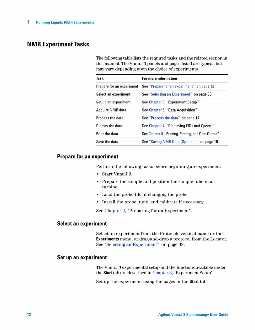
The following table lists the required tasks and the related section in this manual. The VnmrJ 3 panels and pages listed are typical, but may vary depending upon the choice of experiments.
Task For more information
Prepare for an experiment See “Prepare for an experiment” on page 12
Select an experiment See “Selecting an Experiment” on page 38
Set up an experiment See Chapter 3, “Experiment Setup”
Acquire NMR data See Chapter 5, “Data Acquisition”
Process the data See “Process the data” on page 14
Display the data See Chapter 7, “Displaying FIDs and Spectra”
Print the data See Chapter 8, “Printing, Plotting, and Data Output”
Save the data See “Saving NMR Data (Optional)” on page 16
Prepare for an experiment
Perform the following tasks before beginning an experiment:
• Start VnmrJ 3.
• Prepare the sample and position the sample tube in a turbine.
• Load the probe file, if changing the probe.
• Install the probe, tune, and calibrate if necessary.
See Chapter 2, “Preparing for an Experiment”.
Select an experiment
Select an experiment from the Protocols vertical panel or the Experiments menu, or drag-and-drop a protocol from the Locator. See “Selecting an Experiment” on page 38.
Set up an experiment
The VnmrJ 3 experimental setup and the functions available under the Start tab are described in Chapter 3, “Experiment Setup”.
Set up the experiment using the pages in the Start tab.
Agilent VnmrJ 3 Spectroscopy User Guide

Running Liquids NMR Experiments 1
Agilent VnmrJ 3 Spectroscopy User Gui
1 Select the Standard page.
a Fill in the information for the sample, select a Solvent, and enter the comments.
b Enter a name in the Sample Name field to name the sample.
c Define the sample, if desired, by filling in the optional Lot Number, Notebook, Page, Eaddr, and Comment fields.
d Insert the sample.
2 Regulate spinning and temperature on the Spin/Temp page.
3 Find Z0 and adjust the lock using the Shim and Lock pages.
4 Shim the system to adjust the field homogeneity using the controls provided on the Shim page.
de 13

1 Running Liquids NMR Experiments
Acquire a spectrum
14
VnmrJ 3 NMR data acquisition and the functions provided under the Acquire tab are described in Chapter 5, “Data Acquisition”. Set acquisition and acquire data using the pages in the Acquire tab.
1 Set up experimental parameters and post acquisition actions.
2 Click the Acquire button to acquire NMR data.
Process the data
VnmrJ 3 NMR data processing and the functions accessed by clicking on the Process tab are described in Chapter 6, “Processing Data”.
Display the data
VnmrJ 3 data display is described in Chapter 7, “Displaying FIDs and Spectra”. Click the Process tab and select the Display page and the graphic control buttons to manipulate the display of the data.
Agilent VnmrJ 3 Spectroscopy User Guide

Running Liquids NMR Experiments 1
Print or plot the data
Agilent VnmrJ 3 Spectroscopy User Gui
VnmrJ 3 data display is described in Chapter 8, “Printing, Plotting, and Data Output”. Use the Plot page to create a print or plot.
de 15

1 Running Liquids NMR Experiments
Saving NMR Data (Optional)
16
If the data is acquired and the Automatic FID save feature in the Future Actions page under the Acquire tab is not selected, use the Save As window, the Auto Save option, or the Future Actions page to save the data.
Method Description
Future Actions page Click the Acquire tab, Future Actions tab, and Save FID Now button
Main VnmrJ 3 menu options
Click File.Select either Save as or Auto Save. Selecting Auto Save saves the data as specified in Edit/Preferences.Use the Edit/Preferences window to customize where and under what name data is saved (see the VnmrJ 3 Installation and Administration manual).VnmrJ 3 default data saving templates include DATE (producing filenames such as 20040921_01.fid), and seqfil (for example, HMQC_01.fid).
Agilent VnmrJ 3 Spectroscopy User Guide

Running Liquids NMR Experiments 1
Stopping an Experiment
Agilent VnmrJ 3 Spectroscopy User Gui
There are four ways to stop an experiment:
• Click the Stop button.
• Click Acquisition in the main menu, then Abort Acquisition.
• Click the Stop button in the Action bar (when either the Start or the Acquire panel is selected).
• Enter aa on the command line.
de 17

18
1 Running Liquids NMR Experiments
Agilent VnmrJ 3 Spectroscopy User Guide

Agilent VnmrJ 3 SpectroscopyUser Guide
2Preparing for an Experiment
Starting VnmrJ 3 20
Preparing the Sample 21
Ejecting and Inserting the Sample 24
Loading a Probe File 26
Tuning Probes on Systems with ProTune 27
Tuning Probes on Standard Systems 31
This chapter describes how to prepare for an experiment by preparing the sample, ejecting and inserting the sample, loading a probe file, and tuning probes on systems with ProTune or on standard systems.
19Agilent Technologies

2 Preparing for an Experiment
Starting VnmrJ 3
20
1 Log in to the workstation.
2 Double-click the VnmrJ 3 icon.
Agilent VnmrJ 3 Spectroscopy User Guide

Preparing for an Experiment 2
Preparing the Sample
Agilent VnmrJ 3 Spectroscopy User Gui
Sample preparation and positioning in the turbine affects the efficiency of the auto shimming methods. Variations in bulk magnetic susceptibility at air-to-glass, glass-to-solvent, and solvent-to-air contact points can greatly degrade the field homogeneity from sample to sample. The time spent on shimming, or even the need to shim, is largely dependent upon the care in controlling the effects of these contact points.
Selecting a solvent
Most samples are dissolved in a deuterated solvent that does not react or degrade the sample. The instrument can be run unlocked if the sample must be run using a solvent that is not deuterated.
Setting the sample height
Experimentation and calculation show that the length of the liquid column must be at least three times the length of the observe coil window to minimize end effects (for a 5-mm tube in a 5-mm probe). A typical sample length is 5 cm (for 5 and 10-mm probes; it is a bit less for 3-mm sample tubes). Solvent volumes of 0.6 ml in a 5-mm tube and 3.1 ml in a 10-mm tube are adequate for removing the end effects. See the manual provided with the probe in use for specific sample height and volume specifications.
Reduction of sample volume to attain higher concentration usually fails (special plugs for low volume samples are available and will help with line shape) because the increased signal is found around the base of the NMR resonance, not within the narrow portion of the signal. In fact, a well-shimmed 0.4 ml sample will be lower in sensitivity than the same solution diluted to 0.6 ml and also shimmed well. The questionable gain in sensitivity is further degraded by the longer time it will take to shim the system. Small variations of sample height, which would be insignificant in a 0.6 to 0.8 ml sample, can be dominant when the sample is only 0.4 ml in volume.
For best results and reduced shimming times, samples should be prepared to each have the same liquid height as much as possible. Above 0.7 ml, there is little sensitivity to sample length, as long as the bottom of the tube is positioned properly. Prepare every sample up to the same height and obtain shim values using samples of that height.
de 21
22
2 Preparing for an Experiment
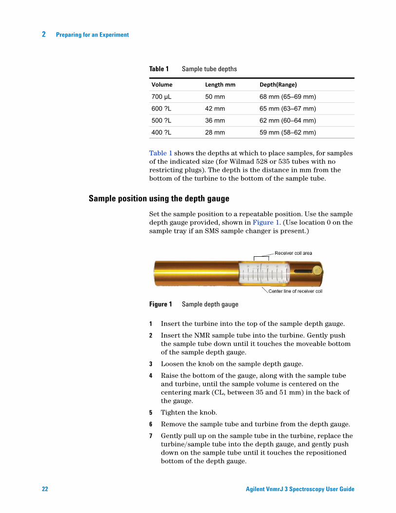
Table 1 shows the depths at which to place samples, for samples of the indicated size (for Wilmad 528 or 535 tubes with no restricting plugs). The depth is the distance in mm from the bottom of the turbine to the bottom of the sample tube.
Table 1 Sample tube depths
Volume Length mm Depth(Range)
700 µL 50 mm 68 mm (65–69 mm)
600 ?L 42 mm 65 mm (63–67 mm)
500 ?L 36 mm 62 mm (60–64 mm)
400 ?L 28 mm 59 mm (58–62 mm)
Sample position using the depth gauge
Set the sample position to a repeatable position. Use the sample depth gauge provided, shown in Figure 1. (Use location 0 on the sample tray if an SMS sample changer is present.)
1 Insert the turbine into the top of the sample depth gauge.
2 Insert the NMR sample tube into the turbine. Gently push the sample tube down until it touches the moveable bottom of the sample depth gauge.
3 Loosen the knob on the sample depth gauge.
4 Raise the bottom of the gauge, along with the sample tube and turbine, until the sample volume is centered on the centering mark (CL, between 35 and 51 mm) in the back of the gauge.
5 Tighten the knob.
6 Remove the sample tube and turbine from the depth gauge.
7 Gently pull up on the sample tube in the turbine, replace the turbine/sample tube into the depth gauge, and gently push down on the sample tube until it touches the repositioned bottom of the depth gauge.
Figure 1 Sample depth gauge
Agilent VnmrJ 3 Spectroscopy User Guide

Preparing for an Experiment 2
Sample tubes
Agilent VnmrJ 3 Spectroscopy User Gui
Buy the best quality NMR sample tubes and clean the outside of each tube with a solvent such as isopropyl alcohol, followed by a careful wiping with a wiper tissue before placing the tube in the probe. Fingerprints left on the sample turbine (in particular) will get transferred into the spinner housing and eventually create difficulties in spinning samples.
Sample changes and probe tuning
Probe tuning is required when there is a significant change in the polarity of the solvent. Changing from a non-polar organic solvent to a more polar organic solvent or aqueous solvent generally requires retuning the probe. Changes in the ionic strength of the solution (for example, low salt to high salt) also require retuning of the probe.
de 23
2 Preparing for an Experiment
Ejecting and Inserting the Sample
24
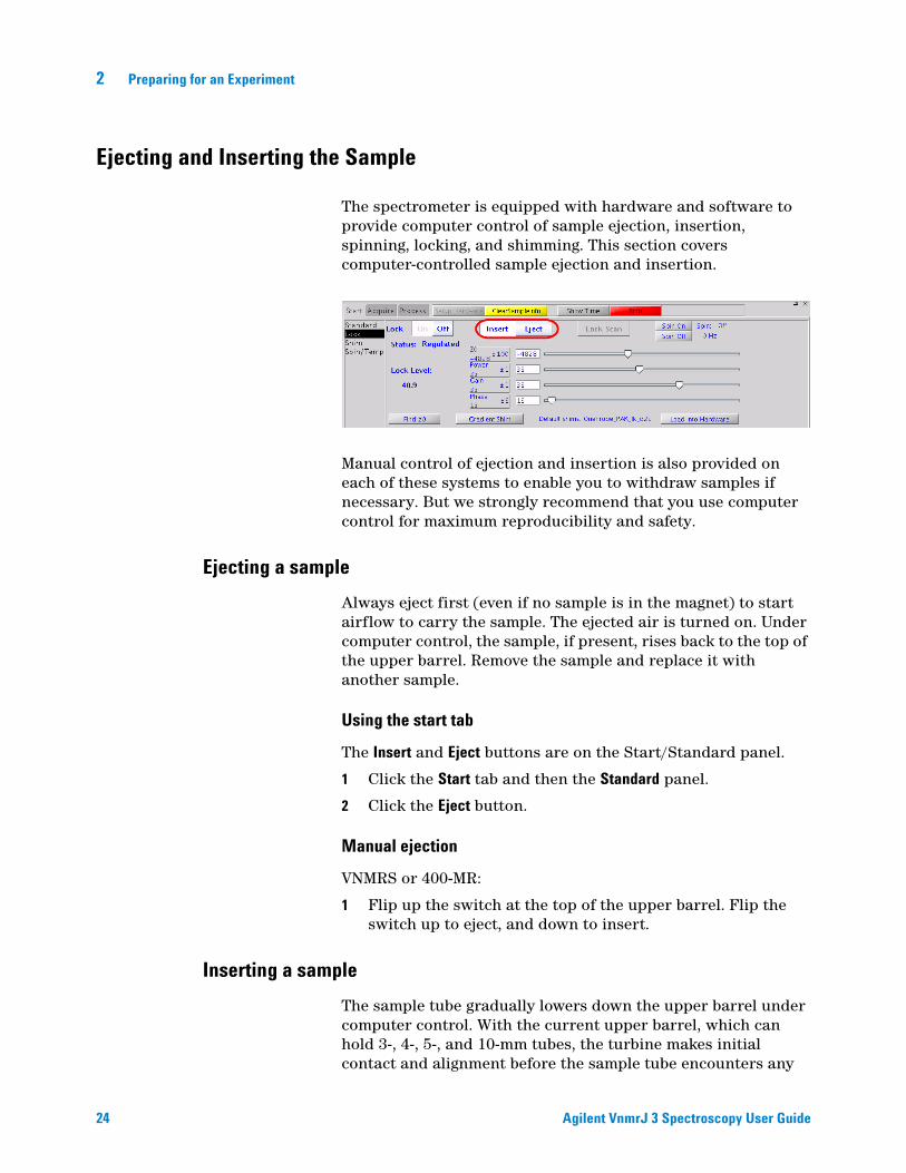
The spectrometer is equipped with hardware and software to provide computer control of sample ejection, insertion, spinning, locking, and shimming. This section covers computer-controlled sample ejection and insertion.
Manual control of ejection and insertion is also provided on each of these systems to enable you to withdraw samples if necessary. But we strongly recommend that you use computer control for maximum reproducibility and safety.
Ejecting a sample
Always eject first (even if no sample is in the magnet) to start airflow to carry the sample. The ejected air is turned on. Under computer control, the sample, if present, rises back to the top of the upper barrel. Remove the sample and replace it with another sample.
Using the start tab
The Insert and Eject buttons are on the Start/Standard panel.
1 Click the Start tab and then the Standard panel.
2 Click the Eject button.
Manual ejection
VNMRS or 400-MR:
1 Flip up the switch at the top of the upper barrel. Flip the switch up to eject, and down to insert.
Inserting a sample
The sample tube gradually lowers down the upper barrel under computer control. With the current upper barrel, which can hold 3-, 4-, 5-, and 10-mm tubes, the turbine makes initial contact and alignment before the sample tube encounters any
Agilent VnmrJ 3 Spectroscopy User Guide
Preparing for an Experiment 2
Agilent VnmrJ 3 Spectroscopy User Gui
close tolerance.
Using the start tab
1 Perform a sample ejection (even if no sample is in the magnet) to start airflow to carry the sample.
2 Insert the sample by placing it in the top of the upper barrel.
3 Click the Start tab.
4 Select the Standard panel.
5 Click Insert.
Manual insertion
VNMRS or 400MR:
Flip down the switch at the top of the upper barrel. (Flip the switch down to insert, and up to eject)
de 25

2 Preparing for an Experiment
Loading a Probe File
26
Probe files can be created at any time and are typically created during system or probe installation. Procedures for creating probe files and probe calibration files are provided in the VnmrJ 3 Installation and Administration manual. For more information on Using Probe ID, see “Calibrating the Probe” on page 70.
1 Click the Probe button on the Hardware bar (bottom left corner of the VnmrJ 3 interface).
The probe selection window appears.
2 Click on the pull-down menu at the top of the Current Probe section in the popup window and select the desired probe file.
3 Click Close to dismiss the window.
Figure 2 Calibrating a probe
Agilent VnmrJ 3 Spectroscopy User Guide

Preparing for an Experiment 2
Tuning Probes on Systems with ProTune
Agilent VnmrJ 3 Spectroscopy User Gui
This section applies to Agilent NMR Systems spectrometers equipped with ProTune.
Configuring for operation with automated sample handlers
• Applies to systems equipped with ProTune.
• The system must be properly configured and ProTune-calibrated. See the VnmrJ 3 Installation and Administration for configuring the software and calibrating ProTune.
1 Log in as the account administrator and start VnmrJ 3.
2 Use the Tuning check box on the Start panel.
3 Gradient shimming will start after each auto tune event if both auto tune and gradient shimming are selected.
The tune protocol (wtune) is specified in the probe file.
Running ProTune on systems not using automated sample handlers
1 Click the Tools button on the main menu bar.2 Select Tune Probe from the menu.
3 To select a nucleus not in the above list, or to select a different criterion: Select a criteria from the drop-down menu next to Tune Criterion in the Advanced Tune section:
Coarse – within 5 percent of optimum pw
Medium – within 2 percent of optimum pw
Fine – within 0.5 percent of optimum pw
de 27
28
2 Preparing for an Experiment
The criteria function is available to the operator depending on the value set in the parameter panellevel.
4 Select the next nucleus and repeat. Continue to the next step when all desired tuning is completed.
5 Click Close to exit the Tune Probe module.
Remote tuning from the ProTune window
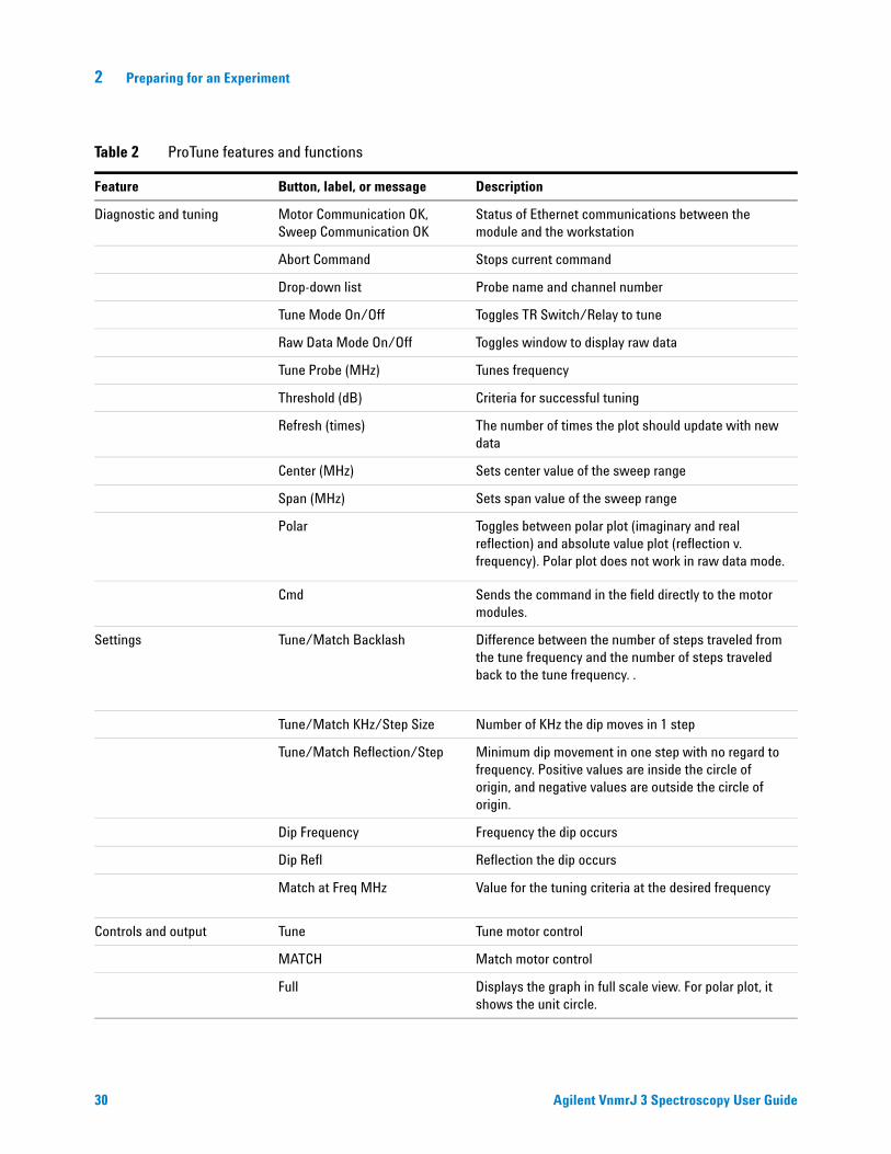
The ProTune interface window (shown in Figure 3 on page 29) can also be used to tune the probe. Functions and features of ProTune are listed in Table 2 on page 30.
1 Start ProTune by entering the following in the VnmrJ 3 command line:
protune('calibrate')
The calibration files for the probe shown on the hardware bar of the VnmrJ 3 interface are loaded. See Figure 4 on page 32.
2 Click the Refresh button.
3 Make sure that the motor and sweep communication read OK before starting manual tuning after the ProTune window appears.
Figure 3 on page 29 shows the ProTune window.
4 Enter the frequency (MHz) in the Tune Probe field.
5 Click the Tune Probe.
Agilent VnmrJ 3 Spectroscopy User Guide

Preparing for an Experiment 2
Agilent VnmrJ 3 Spectroscopy User Gui
The software reads the appropriate channel file and starts tuning.
6 Do the following to stop the automatic tuning and tune manually:
a Click the Abort button.
b Select the appropriate frequency range/channel from the drop-down list.
c Click the appropriate plus or minus buttons to adjust the tune and match.
d Enter a frequency in the Center box and click Refresh to update the reflection window to center the window.
e Enter a frequency width in the Span entry box and click Refresh to update the reflection window to set the window span.
7 Close the ProTune window — acquisition will stop automatically.
Figure 3 ProTune software interface example
de 29
2 Preparing for an Experiment
Table 2 ProTune features and functions
Feature Button, label, or message Description
Diagnostic and tuning Motor Communication OK, Sweep Communication OK
Status of Ethernet communications between the module and the workstation
Abort Command Stops current command
Drop-down list Probe name and channel number
Tune Mode On/Off Toggles TR Switch/Relay to tune
Raw Data Mode On/Off Toggles window to display raw data
Tune Probe (MHz) Tunes frequency
Threshold (dB) Criteria for successful tuning
Refresh (times) The number of times the plot should update with new data
Center (MHz) Sets center value of the sweep range
Span (MHz) Sets span value of the sweep range
Polar Toggles between polar plot (imaginary and real reflection) and absolute value plot (reflection v. frequency). Polar plot does not work in raw data mode.
Cmd Sends the command in the field directly to the motor modules.
Settings Tune/Match Backlash Difference between the number of steps traveled from the tune frequency and the number of steps traveled back to the tune frequency. .
Tune/Match KHz/Step Size Number of KHz the dip moves in 1 step
Tune/Match Reflection/Step Minimum dip movement in one step with no regard to frequency. Positive values are inside the circle of origin, and negative values are outside the circle of origin.
Dip Frequency Frequency the dip occurs
Dip Refl Reflection the dip occurs
Match at Freq MHz Value for the tuning criteria at the desired frequency
Controls and output Tune Tune motor control
MATCH Match motor control
Full Displays the graph in full scale view. For polar plot, it shows the unit circle.
30 Agilent VnmrJ 3 Spectroscopy User Guide

Preparing for an Experiment 2
Tuning Probes on Standard Systems
Agilent VnmrJ 3 Spectroscopy User Gui
Typically, probes are tuned using the Tune Interface shown in Figure 34 on page 187.
Selecting correct quarter-wavelength
When a large change is made in the frequency of the observed nucleus on broadband stems, such as switching from 13C to 15N, an additional change is made in the quarter-wavelength cable—a coiled cable located on the system, as follows:
• Attached to the preamplifier housing for VNMRS spectrometers
• Attached to the inner face of the magnet console interface unit as part of the observe circuitry on other systems
The quarter-wavelength cable is not changed for each nucleus, but only for broad ranges of frequencies (for example, 40 to 80 MHz), it usually changes, covering a factor of two (an octave) in frequency. An incorrect cable does not typically affect signal-to-noise, but may have a profound effect on the 90° pulse length.
Note that ProTune probes have a universal quarter-wavelength cable that spans the entire range of X nuclei. When this cable is used, it never needs to be changed (at least when the probe is connected to ProTune).
Tuning using Mtune
The Mtune routine runs in the graphics canvas and uses VnmrJ 3 panels. Start Mtune as follows:
1 Click Tools on the main menu.
2 Select Manual Tune Probe or enter mtune on the command line.
3 Select the center frequency of the nucleus to tune.
For example, set H1 on channel 1.
4 Select Start Probe Tune on the Mtune panel, see Figure 6 on page 34.
de 31

32
2 Preparing for an Experiment
5 Optional: Choose an appropriate tuning Power (may be channel dependent)–typical values are between 0 and 10 dB.
6 Optional: Set the tuning Gain to 50dB (a typical gain).
7 Set a Frequency Span that shows the tuning dip in full size:
A typical Frequency Span for 1H is 10 MHz.
The Frequency Span for lower frequencies (like 15N) may be 10 MHz, or less if desired. Wider spans may be desired when tuning manually over a wide frequency range.
8 Adjust any of the parameters as needed.
9 Set one or two markers.
Up to two frequency markers are selectable. This is useful for tuning H1 and 19F at the same time, for example with double-tuned coils like in the ATB or 4-nucleus probe families (Figure 5 on page 33).
a Click the Center frequency to markers button to set the tuning frequency in between the two cursors.
b Set the Span to a sweep width that covers both dips. A span of 50 MHz is typical for showing both 1H and 19F at 400 MHz, as shown in Figure 5 on page 33. Maximize the graphics canvas horizontally to have the best screen resolution.
Figure 4 Manual tuning panel
Agilent VnmrJ 3 Spectroscopy User Guide

Preparing for an Experiment 2
Agilent VnmrJ 3 Spectroscopy User Gui
10 Click the Autoscale button to fit the tuning dip vertically into the graphics canvas or scale.
11 Shift the display manually using the Vertical scale/ Vertical Position controls.
12 Keep the default number of acquired points, or change the number of points by selecting a new value from the # Points drop-down menu.
Increasing the number of points provides better resolution at large spectral widths. Higher resolutions will have smaller update rates.
13 Tune the other channels as follows:
• Switch tuning off by selecting Stop Probe Tune.
• Select a different channel and nucleus.
• Switch tuning back on by selecting Start Probe Tune.
14 Repeat Step 1 through Step 13 for each channel.
15 Exit Mtune after tuning is done:
Click Stop Probe Tune, then click Quit to return to the previous NMR experiment.
Figure 5 Frequency span display showing both 19F and 1H tune dips
Tuning using TUNE INTERFACE remote
Using the interface remote
The TUNE INTERFACE remote is attached to the RF front-end and can be extended to the magnet while tuning the probe.
de 33

34
2 Preparing for an Experiment
• The TUNE INTERFACE display, a rectangular liquid-crystal display that shows a numerical value two ways—as a digital readout and as an analog representation along the oval surrounding the digital readout at the top of the screen.
• Two single-digit readouts labeled CHAN and ATTEN are below the display. The CHAN readout can be set to 0 for OFF or to the channel being tuned (1, 2, 3, etc.), and the ATTEN readout is the amount of attenuation (analogous to the TUNE LEVEL knob on older systems). The attenuation is selected in units of 10 dB. The maximum attenuation is 79 dB, which is selected by a setting of 8. (A readout value of 9 is functionally identical to a value of 8.) The buttons above and below each readout allow you to change the value of the readout.
Tuning a probe
Tuning a probe using the TUNE INTERFACE remote involves the following steps:
1 Set up the spectrometer to observe the nucleus of interest.
Often, the system is already set to the correct nucleus; if not, proceed as if to set up an experiment.
2 Set the nucleus for each channel.
The TUNE INTERFACE remote will not work after either powering on or resetting the acquisition console until the tune frequencies are set.
3 Type su.
When a su is executed, the console frequency is set for each channel that is defined for the experiment. This frequency is also used for tuning (in this mode). The table below shows the relationships between the channel selected and the associated parameters:
Figure 6 TUNE INTERFACE remote
Agilent VnmrJ 3 Spectroscopy User Guide

Preparing for an Experiment 2
Agilent VnmrJ 3 Spectroscopy User Gui
See the Command and Parameter Reference for descriptions of these parameters.
4 Press the CHAN buttons until the readout is the number of the RF channel to tune. Start with channel 1.
This turns on the tuning function for the channel. The TUNE INTERFACE display should show a number, and the red indicator light should not flash. (If the light flashes, check the connector to the cable for an improper connection.)
5 Press the ATTEN buttons until the readout is 6, 7, or 8.
6 Optional: Insert the appropriate sticks into the probe if necessary. See the probe installation manual to choose the sticks that are needed to tune to the desired nucleus.
7 Tune the probe. As the probe gets closer to being tuned, the number on the TUNE INTERFACE display will decrease.
8 Press the ATTEN button until the readout is 8, to increase the tuning level sensitivity. Continue tuning until the number displayed on the TUNE INTERFACE display is at a minimum. (The minimum will be around 50-60 for VNMRS-generation console.)
9 Disconnect the tuning function by pressing the CHAN buttons until the readout is 0. (During normal operation, CHAN must be set to 0 or acquisition is not allowed.)
10 Repeat the steps above for each channel on the system.
For further information about probe installation and tuning, see the probe installation manual that was shipped with your probe.
Channel 1 tn Sfrq Tof
Channel 2 dn Dfrq Dof
Channel 3 dn2 dfrq2 dof2
Channel 4 dn3 dfrq3 dof3
de 35

36
2 Preparing for an Experiment
Agilent VnmrJ 3 Spectroscopy User Guide

Agilent VnmrJ 3 SpectroscopyUser Guide
3Experiment Setup
Selecting an Experiment 38
Spinning the Sample 40
Setting the Sample Temperature 45
Handling Spin and Temperature Error 48
Working with the Lock and Shim Pages 49
Optimizing Lock 52
Adjusting Field Homogeneity 58
Selecting Shims to Optimize 61
Shimming on the Lock Signal Manually 63
Shimming PFG Systems 69
Calibrating the Probe 70
Using Probe ID 73
This chapter sequentially describes how to set up experiments by selecting an experiment, spinning the sample, setting the sample temperature, handling spin and error temperature, working with lock and shim, optimizing lock, adjusting field homogeneity, selecting shims to optimize, shimming on the lock signal manually, shimming PFG systems, and calibrating the probe.
37Agilent Technologies

3 Experiment Setup
Selecting an Experiment
38
This section describes using the Protocol window, the menu bar, the Locator, and the Browser to choose and load an experiment. After an experiment is selected, VnmrJ 3 reads and loads the standard parameters, reads the probe file, then loads the probe calibrations.
Protocols window
1 In the left vertical windows, select the Protocols/Experiment Selector.
2 Click an experiment to open in the active viewport.
Main menu selections
NOTE If a study is not selected, the experiment parameters will go into the active viewport, rather than into the StudyQ.
Experiment
1 Click Experiments in the menu bar.
2 Click an experiment in the list to bring it into the active viewport, see the Experiments menu.
The list of experiments contains some submenus.
File
1 Click File.
2 Select Open.
3 Navigate to the directory containing the experiment or data set.
4 Click an experiment or data set from the Browser to a viewport.
5 Click Open to bring it into the active viewport.
Agilent VnmrJ 3 Spectroscopy User Guide

Experiment Setup 3
Agilent VnmrJ 3 Spectroscopy User Gui
Locator
1 Click Tools.
2 Select Locator.
3 Click and drag an experiment from the locator to a viewport or double-click the experiment to bring it into the active viewport.
Browser
1 Click Tools.
2 Select Browser.
3 Navigate to the directory containing the experiment or data set.
4 Click and drag an experiment or data set from the Browser to a viewport.
NOTE Loading a data set does not set parameter values from the current probe file. So, the settings may be incorrect for any new acquisition.
de 39
3 Experiment Setup
Spinning the Sample
40
When the Spin/Temp page under the Start tab is selected, the Liquids Spinner panel or the MAS Spinner panel, depending on the spectrometer hardware, is displayed.
Liquids spinner
To configure the software so that the Liquids Spinner panel is displayed, select a probe file in which the parameter Probespintype has been set to liquids. Optionally, set spintype='liquids' to show the Liquids Spinner panel.
Adjust the spin rate using the Input window or the Acquisition window. Typical spin rates are 20 for 5-mm tubes and 15 for 10-mm tubes.
The last entered spin rate is used to regulate sample spinning when a new sample is inserted. The actual spin rate is indicated in three ways:
• The Spin chart display button on the hardware bar displays a history of the sample spin rate.
• The Acquisition Status window shows the actual rate as well as a spin regulation indication.
• The remote status unit signals the spin rate using the spin light status:
• off — the sample is not spinning.
• blinking — the sample is spinning but not at the requested rate.
• on steady — the spin rate is being regulated at the requested rate.
Using the start tab
The Spin/Temp page is under the Start tab.
Agilent VnmrJ 3 Spectroscopy User Guide

Experiment Setup 3
Agilent VnmrJ 3 Spectroscopy User Gui
1 Click the Start tab. Select the Spin/Temp page.
The controls for the spinning speed consist of an entry field, a slider bar, and a button for disabling or enabling spinning.
2 Adjust the spinning speed with any of these methods:
• Enter a spin rate in the text entry field.
• Drag the slide control. The value changes proportionally as the mouse moves.
• Click in the slider bar to move the slider by one increment.
3 Optional:
• Specify preferences for the control of spinner and temperature by selecting the Control spinner from this page only and Control temperature from this page only check boxes. This forces all spinner and temperature changes to happen from this panel (rather than the command line or some other window). This is a recommended option, and prevents unintended changes in temperature or the spin rate.
4 Specify error handing for spinner and temperature by selecting one of the three options under each of the spinner and temperature sections.
MAS spinner
To configure the software so that an MAS Spinner panel is displayed, select a probe file in which the parameter Probespintype has been set to 'mas'. Optionally, set spintype='mas' to show the MAS Spinner control panel. (For the Nanoprobe, set spintype='tach' instead.)
The MAS Speed Controller controls the flow of the bearing gas according to a linear algorithm based on the speed of the spinning rotor. The bearing pressure profile starts from the final pressure at start up and increases linearly to the maximum bearing pressure in proportion to the speed of the
de 41

42
3 Experiment Setup
rotor. The speed controller already has bearing profiles for all solids spinning modules stored in nonvolatile memory. Use the bearing control items to customize these settings. Changes made to the bearing profile remain in effect until the power is cycled or the probe is changed. To make permanent changes to the bearing profile, use the TIP interface.
WARNING Thinwall rotors can shatter at high speeds, causing injury and damage. If a thinwall rotor is used, be sure that Thin is selected for Rotor Wall.
The MAS Spinner panel (which controls the MAS Speed Controller) is accessed from the Spin/Temp page under the Start tab.
Setting spintype='mas' gives the MAS Spinner control panel described here. Setting spintype='liquids' gives the liquids spinner panel.
Start Button Click the Start button to start the rotor spinning at the target set into the active setpoint.
Stop Button Click the Stop button to initiate the speed controller stop cycle, which slows down the rotor in a controlled manner until it is stopped. The Stop button is intended to provide a normal stop and is not an emergency stop.
Target (Hz) The Target Speed field is used to set the spinning speed stored in the active setpoint. Any changes made to the setpoints remain in effect until the power is cycled or the probe is changed. Setting the target will not start the rotor if it is not spinning, it just sets the value in the setpoint. -- Only the currently active setpoint can be changed. -- If neither setpoint is active, any change made to the value in the Target Speed field activates setpoint one and sets it to that value. -- If the rotor is spinning and the active setpoint is changed, the rotor’s spinning speed changes as soon as the return key is pressed.
Agilent VnmrJ 3 Spectroscopy User Guide

Experiment Setup 3
Probe ID The probe ID is detected automatically by the solids speed controller when the tachometer cable is plugged into the probe. Early solids probes (7.5 mm) had no designated ID type. So, an unplugged cable or a cable plugged into an unknown probe may cause a 7.5 mm probe type to be displayed. Although the probe type is detected immediately by the speed controller when the probe is connected, the probe ID in the panel is updated about once per minute. It is also displayed in the hardware bar.
Current Speed This item displays the current speed of the rotor. This value is also displayed in the hardware bar.
Wall Rotor Displays rotor wall thickness. Setting the Rotor Wall to Thin causes the Max Speed to be reduced to protect the rotor from shattering. The value defaults to Thin after the probe is changed or the controller is reset. If the current rotor is a standard wall rotor, change the setting to Std to get the allowable rotor speed for the probe.
Bearing Adjust (psi) The value in the Adjust field shifts the bearing profile up or down, up to ± 80 psi. The bearing adjustment profile can be a negative number, meaning that the operating profile is lower than the factory setting.
Bearing Span (Hz) The value in the Span field determines when the controller stops following the bearing profile. When the speed of the rotor is within Span Hz, the speed controller freezes the bearing value and does not change it until the spinning speed error exceeds this value. The factory-defined setting for Span is 100 Hz for all spinning modules. When adjusting the bearing profile, set Span to 0, meaning that the bearing pressure is continuously controlled. Then, when finished entering values in the Adjust and Maximum fields, enter a new value in the Span field.
Bearing Max (psi) The value in the Maximum field sets the maximum bearing pressure in psi. This value controls the upper cutoff point in the bearing profile. The maximum bearing pressure is limited to 80 psi.
Active Setpoint Two setpoints are available. The one selected is used to control the speed and is the one that is set when the target is changed. Changing the setpoint while the rotor is spinning immediately changes the target to the value for that setpoint. Selecting None stops the control algorithm and leaves the bearing air and drive air unchanged, which is sometimes referred to as coasting.
Speed Profile Select Active to activate the speed profile feature, which causes the speed controller to constantly compare the drive pressure required to spin the rotor against its preprogrammed estimate of the required pressure for the current speed. If the pressure required to spin the rotor falls outside this range, the speed controller assumes that the rotor is vibrating. If the speed controller cannot stabilize the rotor, it brings the rotor to a stop.
Strip Chart Clicking on the Spin button in the hardware bar will bring up a strip chart of the spinning speed with time.
Agilent VnmrJ 3 Spectroscopy User Guide 43

44
3 Experiment Setup
The following safety measures have been implemented for the high-speed spinner probes (for example, MAS) to prevent rotor and stator damage:
• The air flow selected from the spinner window is ramped to the new value at a safe rate.
• Air flow is shut off if the spinner speed drops to zero, and the spin setting is nonzero to prevent spinner runaway if the tachometer fails.
• Air flow is shut off if, for any reason, the spinning speed cannot be reached to prevent continued attempts to spin a crashed rotor.
Agilent VnmrJ 3 Spectroscopy User Guide

Experiment Setup 3
Setting the Sample Temperature
Agilent VnmrJ 3 Spectroscopy User Gui
Set the temperature for VT control in the Standard page and regulate the temperature by clicking on Spin/Temp page.
See Appendix A, “Status Codes” , for more information on using the Variable Temperature module. The following steps describe a typical operation sequence:
1 Open the Spin/Temp page under the Start folder.
2 Set the desired temperature by entering a value or using the slider, and click Regulate Temp.
3 Set up the acquisition for the experiment as usual, using the Acquire folder.
4 Click the Temp button on the hardware bar to display the temperature display chart.
5 Start temperature control with the Setup Hardware button on the Start folder, or with the Acquire button on the Acquire folder. These commands act as follows:
• Setup Hardware The temperature control and acquisition hardware controls are set and the sample temperature changed to the desired temperature. The experiment is not started when the desired temperature is reached. Wait for the delay time, vtwait, (seconds), then push the Acquire button to begin data acquisition.
• Acquire The same actions occur as in Setup Hardware, except that after reaching the desired temperature, the system waits until the temperature stabilizes, or until the delay time, vtwait, has elapsed (whichever is shorter). Then the pulse sequence and data acquisition begins. The spectrometer waits until the temperature has stabilized, or it waits the delay time, vtwait, (whichever is shorter) every time the temperature is changed under program control.
de 45

46
3 Experiment Setup
Selection of the VT-gas routing occurs after clicking on either Setup Hardware or Acquire. The VT controller begins to control the gas temperature in the probe at the requested temperature. The temperature readout will begin to change, and the VT indicator light will begin flashing. At this time, if the requested temperature is below ambient, either add coolant liquid to the coolant bucket or reset any FTS device to a temperature 10º C or more below the desired operating temperature.
The VT indicator light stays on steadily after the probe temperature reaches the requested temperature (it may initially overshoot). A sample to be studied at non-ambient temperature can now be transferred into the probe. The VT readout is the temperature of the cooling/heating gas as measured just below the RF coil, and this may be slightly different from the true sample temperature. The exact temperature of the sample is correctly determined by a calibration curve that must be constructed for each probe, and must include flow rate and equilibration time. See the VT Accessory Installation manual for the NMR calibration method.
CAUTION Do not use aromatic, ketone (including acetone), or chlorinated solvents in the coolant bucket. Such coolant media attack the standard polystyrene bucket. Another type of container must be used (not supplied by Agilent).
Agilent VnmrJ 3 Spectroscopy User Guide

Experiment Setup 3
CAUTION Operating the system with the coolant bucket filled with liquid nitrogen and with the requested temperature greater than the value of VT cutoff (vtc) results in the condensation of liquid nitrogen inside the exchanger coil tube. If the exchanger coil is then warmed above –210 C or if nitrogen gas is passed through the coil (when temperature is less than VT cutoff), then liquid nitrogen will be forced through the transfer line and into the probe. This will cause a sudden pressure surge in the transfer lines and probe as the liquid nitrogen boils, and it can blow the flexible connector apart. If the liquid nitrogen reaches the glass components of the probe and sample tube, the glass will probably break. Instrument damage can be avoided by following these precautions:
• Do not immerse the exchanger coil in liquid nitrogen when no nitrogen gas is flowing through the coil.
• Do not stop the VT nitrogen gas flow while the exchanger is immersed in liquid nitrogen.
• Arrayed VT experiments that have a temperature range from above VT cutoff to below VT cutoff should be set up starting at the lowest temperature and ending at the highest temperature. When the experiment passes the VT cutoff crossover, remove the liquid nitrogen coolant.
• To avoid water in the exchanger when the low temperature experiment is complete, warm up the exchanger by removing it from the liquid nitrogen and maintain a flow of dry nitrogen until room temperature is reached.
WARNING Sealed samples containing volatile materials can rupture when heated, resulting in potential injury, exposure, and equipment damage. Before running sealed samples at elevated temperatures, heat the samples in an oven at a temperature higher than the highest temperature expected during the experiment. If the tube ruptures while in the probe, the glass components and insert coil will probably be destroyed.
WARNING Sealed samples containing materials with boiling points at or below room temperature can rupture as the sample warms, causing potential injury, exposure, and equipment damage. Equilibrate the probe to a temperature below the sample boiling point before the sample is placed into the probe.
Agilent VnmrJ 3 Spectroscopy User Guide 47

3 Experiment Setup
Handling Spin and Temperature Error
48
Use the Spin/Temp page of the Start tab to select spin and temperature error handling. The provided choices specify the action to be taken if a spinner or temperature failure occurs. Also use the Spin/Temp page to specify whether spinning and temperature can be controlled on panels other than the Start tab.
• Control spinner/temperature from this panel only – prevents the spinner and temperature parameters from being overwritten when old datasets are recalled, but it also locks out control of the temperature from the command line or other panels. Most users prefer to have this option selected.
• Ignore spinner/temperature error – stops any system checking so that acquisition continues regardless of the spin speed or temperature.
• Warn after spinner/temperature error – makes the system check the spin speed and temperature. A warning message is added to the log file if the spin speed or temperature is set to a particular value and the spin speed or temperature goes out of regulation. However, acquisition is not stopped.
• Abort after spinner/temperature error – makes the system check the spin speed and temperature. Acquisition is halted if spin speed or temperature is set to a particular value and the spin speed or temperature goes out of regulation.
Agilent VnmrJ 3 Spectroscopy User Guide

Experiment Setup 3
Working with the Lock and Shim Pages
Mouse control of buttons and sliders
Agilent VnmrJ 3 Spectroscopy User Gui
To change the increment
1 Middle-click the increment button until the desired value is displayed. The defaults are 1, 10, and 100.
2 To change to a customized increment value, shift/middle-click the button, enter a new value, and press Return.
To change the DAC value
1 Enter a new value in the input window and press Return.
2 Alternatively, Shift/left-click the DAC button itself. Enter a new value and press Return.
Lock buttons and controls
The Lock and Shim buttons (z0, Lock Power, Lock Gain, Lock Phase) provide on-the-fly adjustment. The slider values can be moved with the mouse or entered directly.
de 49

3 Experiment Setup
Shim buttons and controls
Working with Proshim
50
Proshim automatically adjusts shim values defined by the selected method on the Proshim panel.
AutoShim Now
Proshim Now Select Proshim Now to call the doproshim macro to send the fgproshim macro to process in the background.
Using Method Select from the provided list of methods to define how Proshim will make adjustments.
Agilent VnmrJ 3 Spectroscopy User Guide

Experiment Setup 3
Skip Lock Adjust Select Skip Lock Adjust to disable automatic lock, gain, power, and phase adjustments.
User-Defined Method Select from the list of user-defined methods to define how Proshim will make adjustments. User-defined method files are added to vnmr/proshimmethods.
Automated Shim Tools
Shim Scheduler Click Shim Scheduler to access the Shim Maintenance Scheduler popup. The scheduler is used to create a Shim.csv file and an associated schedule.
Shim Maintenance Scheduler
Define Sample
Sample Name Enter name for the shimming study
Position Enter the location for the lineshape example
Shim Method Select a Shim method to associate with the shimming study
Create CSV File Click to save Shim.csv to vnmrsys/Spreadsheets
Solvent Select a solvent from the provided listSolvents are typically acetone-d6
Help Click to display help content for the Shim Maintenance Scheduler
Set Shim Time
Day Select the day for Shim service
Hour Select the hour for Shim service
Minute Select the minute for Shim service
Schedule Shim Service
Click to schedule the Shim service
Cancel Shim Service Click to cancel the Shim Service
Auto Lineshape Now Click to acquire a lineshape spectrum with “Z-PFG” shim
Proshim Help Click to display Proshim help content
Abort Proshim Click to stop Proshim
Lock Level Displays current lock level
Agilent VnmrJ 3 Spectroscopy User Guide 51

3 Experiment Setup
Optimizing Lock
52
Under computer control, the lock system maintains a constant field at the sample as the static field generated by the superconducting magnet drifts slowly with time or changes due to external interference. Locking makes the resonance field of the deuterium in the deuterated solvent coincide with the lock frequency.
The lock level can be viewed by clicking on the Lock button on the hardware bar.
The entire lock optimization process can be skipped if optimum lock parameters are already known for a particular solvent and probe combination. Values for these parameters can be entered as part of a macro or by using normal parameter entry (for example, by entering lockgain=30 lockpower=24). These parameters do not take effect until an su, go, or equivalent command is given.
It is important to obtain an optimal lock signal if automatic shimming is to be used. Manual adjustment often is done to achieve the maximum lock amplitude. This can result in a partly saturating condition, and a true non-saturating power is usually 6 to 10 dB lower. The response of the lock level is governed by the T1 of the deuterated lock solvent as well as the magnet-determined or chemical exchange-determined T2 * of the solvent. This can vary widely, from about 6 seconds for acetone-d6 to about 1.5 seconds for CDCl3 and lower for more viscous solvents. To allow a reliable, repeatable selection of lock power, automatic optimization may be used.
Finding Z0 and establishing lock
Find Z0 and establish the lock either manually or by using Autolock (through the Standard page of the Start tab).
Agilent VnmrJ 3 Spectroscopy User Guide

Experiment Setup 3
Agilent VnmrJ 3 Spectroscopy User Gui
Manual method
Establish lock using manual locking on the Lock page. The line that crosses the spectral window represents how close the deuterium resonance field is to the lock frequency. When the two are matched, the line should be flat (with perhaps some noise, depending on the lock gain and lock power). The greater the number of sine waves in the line, the poorer the match.
1 Make sure a sample is inserted and seated properly. Spinning is optional.
2 Click the Lock page in the Start tab.
3 Click either Spin On or Spin Off.
4 Click Lock Scan to open the lock display.
5 Click the Lock Off button. (The lock should not be on and regulated when adjusting Z0.)
6 Find Z0 by clicking on and dragging the Z0 slider bar until the lock signal is on resonance.
7 Adjust the lock power, gain, and phase by clicking on and dragging the slider bars, or by clicking on the buttons.
The actual value needed for lockpower and lockgain depends upon the concentration of the deuterated solvent, the nature of the deuterated solvent—the number of deuterium atoms per molecule—and the relaxation time of the deuterium. At this point, do not be too concerned about optimizing power and gain; just look for a sine wave.
8 Click the ±10 or ±100 button for Z0 until some discernible wave appears if no sine wave (perhaps just noise) is seen.
9 Reduce the lock power if the concentration of the lock solvent is high (>50%).
10 Reduce the lock power if the signal oscillates (goes down and then back up) and it is difficult to establish lock. The deuterium nuclei become “saturated” if the lock power is too high. Acetone is more easily saturated than most solvents.
11 Adjust Z0 until the signal changes from a sine wave to an essentially flat line. The line may start to move up on the
de 53

54
3 Experiment Setup
screen as the lock condition is approached if the solvent is concentrated.
12 Click the Lock On button.
13 Click Lock Scan again to close the lock display.
AutoLock with probe file
This requires a probe file with proper probe calibrations. See the VnmrJ 3 Installation and Administration user guide.
1 Click Find Z0. This button can be found on either the Standard page or the Lock page of the Start tab.
AutoLock
1 Click the Standard page of the Start tab.
2 Click either Spin On or Spin Off.
Select an option for the menu next to the Autolock button.
3 Click the Autolock button — the spectrometer will find Z0 and make all specified adjustments.
4 Choose Find Z0 or AutoLock.
5 Clicking on the button next to opens a drop-down menu of options.
Agilent VnmrJ 3 Spectroscopy User Guide

Experiment Setup 3
Lock power, gain, and phase
Agilent VnmrJ 3 Spectroscopy User Gui
Lock power, gain, and phase are set by the lock parameters—lockpower, lockgain, and lockphase—when using autolock. The parameters set the following limits and step sizes:
• lock power is 0 to 68 dB, step size of 1 dB (68 is full power)
• lock gain is 0 to 48 dB, step size of 1 dB (48 is full gain)
• lock phase is 0 to 360 degrees, step size of 1 degrees.
The Z0 field position parameter z0 holds the current value of the Z0 parameter. The limits of z0 are: -2047 to +2047, in steps of 1, if the parameter shimset is set to 1, 2, or 10, or; -32767 to +32767 if shimset is set to another value.
Lock control methods
Click the Start tab and select the Standard page to access the following lock methods and controls:
Each method is discussed in the following separate sections. Additional sections discuss error handling and lock loop time constant control.
Leaving lock in the current state
Set Autolock to Not Used.
When Autolock is set to Not Used, the freshly inserted sample will lock only if the new sample has the same solvent as the previous sample, and if the values of Z0, lock power, and lock gain have not been re-adjusted.
Running an experiment unlocked
Set Autolock to Unlocked.
Lock is deactivated at the start of acquisition.
Simple Autolock
Set Autolock to Simple.
The system searches for the lock signal and, if necessary, optimizes lock power and gain (but not phase), whenever an acquisition is initiated with go, ga, au or with any macro or menu button using the go, ga, or au if Autolock is set to Simple at the beginning of each experiment (each initiation of an acquisition).
de 55

56
3 Experiment Setup
Find Z0
Find Z0 acquires a 2H spectrum, finds the offset of the tallest peak, and uses that information to set the value of Z0. It does not adjust lock power, lock gain, or lock phase. This option is selected whenever Autolock is set to Every sample or Every expt. However, if the lock is not captured by this method, the system starts using the Autolock Optimization options listed below.
Optimizing Autolock
Optimizing Autolock uses a sophisticated software algorithm to search the field over the full range of Z0 (as opposed to hardware simple Autolock), captures lock, and automatically adjusts lock power and gain (but not lock phase).
• Lock Find Resonance is set to Every Sample.
• The same process as Simple occurs, but only if the sample has just been changed under computer control and acquisition is started (when manually ejecting or inserting a sample, the software cannot keep track of the action and Every Sample has no effect).
• z0 is inactive and when an autolock operation is started, autolock searches for the lock signal by changing the lock frequency.
Spectrometer frequencies are computed from the lock frequency. So, if the lock frequency changes as a result of an Autolock operation, frequencies for that acquisition are off by the amount of that change. Switching from chloroform to acetone requires a change in the lock frequency of about 5 ppm, which is then reflected in the acquired spectrum.
Agilent VnmrJ 3 Spectroscopy User Guide

Experiment Setup 3
Agilent VnmrJ 3 Spectroscopy User Gui
Full optimization
Full optimization is the most complete optimization of lock parameters. A fuzzy logic autolock algorithm automates the parameter control process in order to find the exact resonance and the optimum parameters (phase, power, gain) automatically and quickly with high reliability. Fuzzy rules are used in the program to find the exact resonance frequency and for adjusting power and phase. The fuzzy rules are implemented at different stages of the autolock process. First, the software finds the resonance. If the exact resonance cannot be found, phase and power are adjusted and the software looks for the exact resonance again. The software then optimizes the lock power to avoid saturation, optimizes the lock phase, and optimizes the lock gain to about half-range.
RF frequencies, decoupler status, and temperature are also set during full optimization.
de 57

3 Experiment Setup
Adjusting Field Homogeneity
58
See also Chapter 4, “Gradient Shimming” , if the system is equipped with gradient shimming capabilities.
Shim coils produce small magnetic fields that are used to compensate for inhomogeneities in the static field. In shimming, the current in the shim coils is adjusted to make the magnetic field as homogeneous as possible. Computer-controlled digital-to-analog converters (DACs) regulate the room-temperature shim coil currents. Users should plan to adjust the shims every time a new sample is introduced into the magnet or a probe is changed.
See Appendix 3, “Experiment Setup” , for more information about shimming.
Loading shim values
1 Click the Lock page in the Start panel.
2 Click the Load into Hardware button.
This is the equivalent of the command line instructions: load=’y’ su. Shim values stored in the current experiment are loaded (this may not be suitable).
Loading a shim file
Load a shim set from the Locator to the shim buttons area of the Shim page as follows:
1 Click the Locator Statements button (magnifying glass icon).
2 Select Sort Shimsets. Shim sets can also be sorted by probe or filename.
3 Select a shim set and drag-and-drop it onto the graphics canvas or shim buttons area of the Shim page.
Saving a shim file
Save the shim values to a file as follows:
1 Enter a file name in the field next to the Save Shims button, and press Return.
2 Click the Save Shims button.
Agilent VnmrJ 3 Spectroscopy User Guide

Experiment Setup 3
Shim gradients
Agilent VnmrJ 3 Spectroscopy User Gui
The shims coils are printed coils wrapped around a cylindrical form. The probe slides into the resulting shim tube. A coil (or sum of coils) whose field is aligned along the axis of the magnet is called a Z axial shim gradient (Z1, Z2, Z3, etc.). Coils whose fields are aligned along the other two orthogonal axes are called X and Y radial shim gradients (X1, XY, X2Y2, Y1, YZ, etc.). The field-offset coil Z0 (“zee-zero”) alters the total magnetic field.
Each shim gradient is controlled by its own parameter; for example, the X1 shim gradient is controlled by a parameter named x1.
Depending on the value of the shimset parameter, shim values range from -2047 to +2047 or from -32767 to +32767, with a value of zero producing no current.
Automated shimming on the lock
See “Autoshim Information” on page 495 and both Z3 and Z1 (Z5 not available on 13-channel shim systems), for more information about Autoshim.
Manual shimming on the lock is done with the controls on the Shim page. Automated shimming on the lock is preferred and can be set up from the Standard page of the Start tab:
Shim on Lock options menu next to When:
• Never — disables automatic lock shimming.
• Every sample — shims before the start of data acquisition for each new sample.
• Every Experiment— shims before the start of data acquisition for each new experiment.
• Every FID— shims before the start of data acquisition for each FID.
de 59

60
3 Experiment Setup
Shim on Lock options menu next to Shim method:
• z1z2
• Low non-spins
• All non-spins
• All z’s
• Hi-res z’s
• Fine z1,z2
• Fine z1-z3
Autoshim is controlled by the selection made from the Shim method menu. This is a complete background Autoshim method that provides no interaction with the operator. The type of automatic shimming you should select during routine sample changes depends upon the level of homogeneity required on any particular sample, the change in sample height, and the maximum time desired for shimming.
• z1,z2 shimming — average homogeneity needs, with long samples of identical height.
• all z’s — variable sample heights. More time is required. The method shims first Z1, Z2, and Z4, then Z1, Z2, and Z3, and finally Z1 and Z2.
Agilent VnmrJ 3 Spectroscopy User Guide

Experiment Setup 3
Selecting Shims to Optimize
Which shims to use on a routine basis
Agilent VnmrJ 3 Spectroscopy User Gui
The following suggestions assist in routine shimming, especially on shim systems with a larger number of shim channels:
• Establish and maintain lineshape – Use Z to Z5, possibly Z6, X, Y, ZX, ZY, and possibly Z2X and Z2Y. The effects of Z7 and Z8 (and realistically Z6) are too small to see with the lineshape sample.
• Shim a new lineshape sample of different geometry – Use Z to Z5, possibly Z6, X, Y, ZX, ZY, and possibly Z2X and Z2Y.
• Shim a new sample of the same geometry – Use Z, Z2, and maybe Z3. (Higher field magnets are more likely to need additional Z3 corrections, and eventually even some Z4.)
• Shim a new sample of different geometry – Use Z to Z4 and possibly Z5, X, Y, ZX, ZY.
• Shim for preset water suppression – Start with a shim set that produces a good lineshape for the same sample geometry. Next, tweak Z and Z2, and then vary Z5 and Z7 to minimize the width of the base of the water (Z and Z2 may need to be tweaked if Z5 changes by more than 100 to 200 coarse units). About 80 to 90 percent of the odd-order axial-gradient induced water width is probably dominated by Z5, with Z7 and perhaps some Z3 providing the rest.
The even-order axial shims (Z2, Z4, Z6, and Z8) affect the asymmetry of the residual water line (using presaturation). All four of these even-order axial shims can affect the final water linewidth, with Z2 and Z4 being at about the 5 mM solute level and above, Z6 being at about the 1 mM solute level, and Z8 being at about the 0.3 mM solute level. The even-order axial shims perform as expected except when the sample is less than 40 mm in length, in which case, the shims still control the water linewidth but much less responsively.
Using Z4 to narrow an asymmetric residual water line of a sample shorter than about 40 mm can destroy the base of the standard lineshape faster than the residual water signal is narrowed. The residual water resonance width is affected by magnetic susceptibility interfaces as the sample gets shorter. Iterative use of Z5-Z7 with Z6-Z8-Z4-Z2 can narrow the residual water line for samples under 40 mm. But the
de 61

62
3 Experiment Setup
results obtained may be hard to reproduce on subsequent samples due to an increase in sensitivity to small changes in sample geometry.
Shimming different sample geometries
Some suggestions when moving the sample:
• Moving the same sample up – Z, Z3, and Z5 need to become more positive.
• Shortening and centering (moving up) the sample – Z2 and Z4 need to become much more positive. The trends for Z and Z3 are mixed and more complex, but they tend to become a little more negative. It appears as if Z and Z3 are driven positive as the sample is pulled up, but they are driven negative faster as the sample shortens. When shimming a lineshape sample, plan on the following changes (starting from lineshape shims for a 700 μL sample at a depth 67-68 mm):
700 μL to 600 μL: move Z2 +50 DAC units and move Z4 +250 units. 700 μL to 500 μL: move Z2 +200 units and Z4 +600 units.
The Z2 and Z4 change track well with sample volume, but are relatively independent of tube depth. It is, therefore, easiest when changing sample geometries to make the appropriate Z2 and Z4 corrections, then adjust the more complex Z1-Z3-Z5 interactions as needed.
Agilent VnmrJ 3 Spectroscopy User Guide

Experiment Setup 3
Shimming on the Lock Signal Manually
Agilent VnmrJ 3 Spectroscopy User Gui
Monitor the intensity of the lock signal while adjusting the shim settings. Each shim setting controls the current through shim coils that control magnetic field gradients in different directions. The Z direction must be parallel to the vertical direction of the probe, and it is for this reason that the height of the sample in the NMR tube affects the Z shim settings rather dramatically.
Routine shimming
1 Load the shim settings that have been most recently established for the probe in use as a starting point if the shim settings are way off the mark (for example, if the temperature has changed).
2 Click Setup Hardware.
3 Make sure that:
• the probe has a sample
• it is spinning at the correct speed
• the system is locked onto the deuterium resonance from the lock solvent
4 Check that the lock signal is not saturated. The signal is saturated if changing the lock power by 6 units (6 dB) does not change the lock level by a factor of two. Adjust the lock gain as necessary.
5 Open the Shim page.
Try a change of +10 or -10 in the setting for Z1. If the lock level goes up with one of these, continue in that direction until the level is maximized (it no longer increases, but instead begins to fall).
6 Change the setting for Z2C or Z2 by +10 or -10 and continue in that direction until the level is maximized.
7 Adjust Z1 for maximized lock level, then adjust Z2 for the same. Continue this iterative process until the lock level goes no higher. If the lock level increases to 100, decrease lock gain and then continue to adjust Z1 and Z2. Lock power can be adjusted as needed.
de 63
64
3 Experiment Setup
The routine adjustment is sufficient in most cases. Critical experiments, in some cases, do require adjustment of higher order Z shims and the non-spin shims.
The following procedure is suggested for a second level of shimming:
1 After Z1 and Z2 have been adjusted for maximum lock signal, write down the lock level, adjust Z3 in one direction, by +10, and then repeat the optimization of Z1 and Z2 (iteratively) until the lock signal is at a maximum. Note this level of the lock signal. Continue changing Z3 in the same direction if the lock signal is higher than it was initially. Every change in Z3 must be followed by optimization of Z1 and Z2 until the lock level is at a maximum.
2 Repeat step 1 with Z4. That is, change Z4 in one direction, then optimize Z1 and Z2. If the lock level does not go up, change Z4 in the opposite direction and optimize Z1 and Z2. Continue until the highest possible lock level is obtained.
3 Repeat steps 1 and 2 iteratively until the highest possible lock level is obtained.
4 Turn the spinner off and go through the non-spin shims, one at a time, maximizing the lock level for each one. Then return and go through each again. Continue through all until the lock level is as high as possible. If lock is lost, increase the lock gain.
5 Turn the spinner on and optimize Z1 and Z2 as described above, return to the non-spins (turn the spinner off) and re-optimize these. Continue until the highest lock level is obtained.
Insert the lineshape sample (CHCl3 in deuteroacetone for 1H, and dioxane in deuterobenzene for 13C) for an ultimate check and examine the lineshape to make certain that the homogeneity is close to the original specs, especially for the lineshape at 0.55% and 0.11% of the total peak height. Also examine the height of the spinning sidebands. See the Probe Installation manual that was shipped with your probe.
Agilent VnmrJ 3 Spectroscopy User Guide

Experiment Setup 3
Setting low-order (routine) shims
Agilent VnmrJ 3 Spectroscopy User Gui
The following procedure describes how to set the low-order, or routine, shims. Resetting Z0 and lock phase is normal when making very large changes in the room temperature shims. With this procedure, concentrate on improving the symmetry of the main resonance as well as the half-height resonance and lineshape.
1 Adjust the lock level to about 80 (if possible).
Maximize lock level with Z1.
Maximize lock level with Z1 and Z2. Do this by making a change in Z2 followed by maximizing with Z1 again. Continue to iterate in this manner until there are no further increases in the lock level.
2 Acquire the spectrum.
Resonance lines are symmetric if the sample is properly shimmed.
Resonances that are asymmetric or unusually broad at the base require added attention; see Table 31 on page 406 in Chapter 14, “Data Analysis” , for which shims to adjust. Adjusting Z4 or the non-spins is not required for most routine samples.
3 Adjust Z3 by interactively shimming Z1 and Z3 in the manner described in step 3 for Z1 and Z2. Changes in Z3 may affect Z2. So, after shimming Z3, maximize Z1 and Z2 again.
Removing spinning sidebands (non-routine)
Use this procedure to reduce or eliminate spinning sidebands that are not within specification.
1 Write down the lock level, set SPIN to OFF, and write down the lock level.
2 Adjust lock to about 80 if possible.
3 Maximize lock level with X.
de 65

66
3 Experiment Setup
4 Maximize lock level with Y
5 Maximize lock level with X and Y.
Do this by making a change in Y followed by maximizing with X again. Continue to iterate in this manner until there are no further increases in the lock level.
6 Maximize lock level with X and ZX.
Do this by making a change in ZX followed by maximizing with X again. Continue to iterate in this manner until there are no further increases in the lock level.
7 Maximize lock level with Y and ZY.
Do this by making a change in ZY followed by maximizing with Y again. Continue to iterate in this manner until there are no further increases in the lock level.
8 Repeat step 3 above.
9 Maximize lock level with XY and ZXY (ZXY not available on 13 or 14 channel shim systems).
10 Repeat step 3 through step 5.
11 Set SPIN to ON and acquire a spectrum.
If the sample is properly shimmed, the lines should be symmetric.
12 See Table 45 on page 494 and the previous sections for which shims to adjust if the lines are not symmetric or are unusually broad at the base. For most routine samples, adjusting Z4 or the non-spins is not required.
13 Adjust Z3 by interactively shimming Z1 and Z3 in the manner described in step 3 in the previous procedure (“Setting low-order (routine) shims” on page 65) for Z1 and Z2.
Changes in Z3 may affect Z2. So, after shimming Z3, maximize Z1 and Z2 again.
Agilent VnmrJ 3 Spectroscopy User Guide

Experiment Setup 3
Setting the high-order axial shims (non-routine)
Agilent VnmrJ 3 Spectroscopy User Gui
See “Shim Interactions” on page 489, for information about shim interactions.
1 Look at which side of the peak has asymmetry to determine how to adjust Z4 — low field to the left and high field to the right.
2 Use Figure 111 on page 490, in Appendix B, “Shimming Basics” , to determine which direction to move Z4. A large asymmetry implies that Z4 is far off. Change Z4 by a considerable amount to try to push the asymmetry to the other side of the peak. This provides two important pieces of information:
• Confirms that Z4 is the problem if the asymmetry moves.
• Indicates what the actual value of Z4 should be when Z4 is changed. Because the values that caused it to be on either side of the peak are known, the correct value must be between the two extremes.
3 Set Z4 to the value that produces neither a high-field nor low-field asymmetry.
Z4 affects all the shims below it. So, repeat the procedure “Setting low-order (routine) shims” on page 65.
4 Maximize the lock level with Z5.
5 Repeat step 3 and step 4 until no further increase is obtained.
Setting high-order radial shims (non-routine)
Note that Z2X, Z2Y, ZX2–ZY2, Z3X, Z3Y, and Z5 are not available on 13-channel shim systems.
1 Set SPIN to OFF and write down the new lock level.
2 Set the lock level to about 80.
3 Maximize the lock level by shimming Z2X against ZX.
4 Maximize the lock level by shimming Z2Y against ZY.
5 Repeat the procedure “Removing spinning sidebands (non-routine)” on page 65 .
6 Maximize the lock level by shimming ZXY against XY.
7 Maximize the lock level by shimming ZX2–ZY2 against (X2-Y2).
8 Set SPIN to ON and adjust the lock level to 80.
de 67

68
3 Experiment Setup
9 Maximize the lock level by shimming Z1, Z2, Z4, and then Z1, Z2, Z3.
10 Repeat step 1.
11 Maximize the lock level by shimming X3 against Y3.
12 Maximize the lock level by shimming Z3X against Z3Y if available.
See the installation data for your magnet for approximate Z3X and Z3Y values.
13 Look at the spectrum and decide where to concentrate your effort:
• For a broad base, adjust Z4 and Z5.
• For spinning sidebands, adjust the proper order radial shims. The contribution of Z3 to the breadth of the base becomes evident (as does the contribution from the high-order radial shims) as Z4 and Z5 are optimized. Several cycles of shimming are required.
Local maxima are be encountered from time to time that can cause problems. A local maxima is indicated if a high-order shim continues to increase and eventually reaches the maximum output of the shim supply, without having reached the optimal lock level.
Carefully re-examine the lower-order shims by making large excursions (systematically), beginning with the lowest-order shim and working up. This is a particularly difficult issue when dealing with the high-order radial shims such as X3, Y3, Z3X, and Z3Y, because their perturbation of the lock level is small relative to the change in the shim current.
The effects of X3, Y3, Z3X, and Z3Y on the spectrum are significant in experiments such as water suppression, but can go unnoticed or may not be important in some routine 1D spectra where large solvent peaks are not encountered.
Agilent VnmrJ 3 Spectroscopy User Guide

Experiment Setup 3
Shimming PFG Systems
Agilent VnmrJ 3 Spectroscopy User Gui
These procedures apply to the Performa I, Performa II, Performa IV, and Performa XYZ PFG systems. Once in operation, leave the amplifier powered on to allow the amplifier to reach a long-term equilibrium.
Performa I and Performa II
1 Open the System settings window (Edit > System settings).
2 Next to the Gradient amplifier label, set X, Y, and Z to off. Click OK.
3 Click the Setup Hardware button. This button is available when the Start tab is open.
4 Verify a drop in the lock level from the small dc zero current from the amplifier.
5 Shim the system to the desired level.
6 Open the System settings window and set Gradient amplifier Z to on. Click OK. The shimming changes from the small dc offset current.
7 Click Setup Hardware.
8 Adjust Z1 to restore the homogeneity. The lock level should have identical stability on the meter.
This two-stage approach is not strictly necessary, but it does separate any problems that might arise.
Performa XYZ
1 Prepare the amplifier by moving the switch from STANDBY position to ON.
2 Open the System Settings window (Edit > System settings) and set Gradient amplifier X, Y, and Z to on. Click OK.
3 Click the Setup Hardware button. This button is available when the Start tab is open.
The yellow RUN light should turn on.
de 69

3 Experiment Setup
Calibrating the Probe
70
Probe calibrations are stored in the probe file. Use these procedures and the standard calibration samples to update and maintain the calibration file for the probe. See the VnmrJ 3 Installation and Administration user guide for detailed instructions on automatic and manual probe calibration procedures.
Using auto calibration procedures
Do one of the following to start the probe calibration (see Figure 7) and open the probe window:
Use the main menu bar
1 Click Tools.
2 Select Standard Calibration Experiments.
3 Select Calibrate Probe.
Use the hardware bar
1 Click the Probe button.
2 Select Setup Calibration.
Figure 7 Calibrating a probe
Agilent VnmrJ 3 Spectroscopy User Guide

Experiment Setup 3
Agilent VnmrJ 3 Spectroscopy User Gui
3 Click the Do Calibration button in the probe calibration popup window.
4 Select Calibrations from the calibration popup window.
5 Click a radio button in the Calibrate Probe window to select the calibration experiment, see Figure 8.
6 Enter the location of the calibration sample.
No entry field appears if a sample changer is not attached to system.
7 Insert the sample into the magnet manually using the insert and eject button located on the Lock page of the Start tab if a sample handler is not present or not used.
8 Select Autolock (YES or NO).
9 Click the NO button if the sample is already locked or to lock manually.
10 Select Autoshim (YES or NO).
11 Click the NO button if the sample is already shimmed or to shim manually.
12 Click the Start Calibration button.
Follow the online instructions and see the VnmrJ 3 Installation and Administration user guide for detailed instructions on automatic and manual probe calibration procedures.
Figure 8 Calibrate probe window
de 71

72
3 Experiment Setup
Some probes, like the Autoswitchable and 4 nucleus probes, require additional calibrations not covered in this manual. For information on the calibration of these probes, see the installation, testing, and specifications manual for the probe.
Using manual calibration procedures
See the manual calibration section of the VnmrJ 3 Installation and Administration user guide and the acceptance test procedures supplied with the probe.
Agilent VnmrJ 3 Spectroscopy User Guide

Experiment Setup 3
Using Probe ID
Agilent VnmrJ 3 Spectroscopy User Gui
Probe ID is a feature that provides several kinds of enhancements to the use of probe files. It was introduced in VnmrJ 3.1, and can be used only if the appropriate hardware is present. The user has the ability to enable and disable Probe ID as desired.
To use Probe ID, the console must be equipped with a Network Attached Probe Unit. This unit (a small black box) is connected to a power supply and to the console’s Ethernet switch (all of which are located within the console cabinet). A USB cable connects a flash drive integrated into the NMR-probe’s base to the Network Attached Probe Unit. (To use Probe ID on older probes, the user will need to provide an appropriately formatted thumb drive -- one which has the correct specifications.)
Probe ID allows the factory to store probe specifications, calibrations, and probe-test data on the probe itself. This allows the probe-specific data to always remain with the probe. Probe ID allows the installer to backup the installation calibrations onto the probe for safekeeping, and to refer to the factory information as needed. Probe ID allows the user to protect the spectrometer from mis-configuration and see probe specifications for the installed probe (which facilitates re-calibrations).
Probe files have an identity as being either “Probe ID” or “non-Probe ID”, depending upon which identity the user (or installer) gave them when they were created. The calibration procedure is identical for each type of probe file. (See the VnmrJ 3 Installation and Administration user guide for detailed instructions on automatic and manual probe calibration procedures.) The user can decide whether to enforce the use of Probe ID or not..
Probe ID present / not present
The configuration popup, which can only be accessed by vnmr1 (in Edit / System Settings / System config, see the VnmrJ 3 Installation and Administration user guide for details) has a pull-down menu for Probe ID that sets whether the Probe ID software is either “present” or “not present”. If it is set to “present”, then all users can access the settings that let each user “Use Probe ID” or not. This latter choice is determined by the check boxes at the top of the Probe pop-up window.
de 73

3 Experiment Setup
Probe ID “not present” – for older consoles or probes without Probe ID
74
If Probe ID is not installed on a system, the Probe ID field in the “Manage Probe Files” window is fixed as, “Probes without ID.” See Figure 9. Probe ID Enforce or Disable Modes
Figure 9 Probe ID “not present”
Probe ID Enforce or Disable modes
When Probe ID is inserted on a system with a Probe ID compatible probe connected, the user has the choice to use Probe ID in either the “Enforce” or “Disable” modes. Toggling between these two modes is accomplished by selecting either “Enforce Probe ID” or “Disable Probe ID” from the Tools menu. See Figure 10.
Agilent VnmrJ 3 Spectroscopy User Guide

Experiment Setup 3
Agilent VnmrJ 3 Spectroscopy User Gui
When in “Disabled” mode, the system behaves as if Probe ID was not present. All accessible probe files will be displayed in the Current Probe pull-down menu and the user is free to choose any of these probe files.When in “Enforce” mode, Probe ID filters all the available probe file choices based on the value of the probe identification number and displays only those probe files whose Probe ID number matches that of the probe physically attached to the system. Furthermore, “Enforce” mode requires that the probe physically attached to the system match the probe identification number in the probe file. If this is not the case, the system will abort any attempt to acquire data and display an error message in the Probe Popup window.
Figure 10 Probe ID Enforce/Disable
de 75

76
3 Experiment Setup
The features and benefits of Probe ID
The use of Probe ID offers numerous features and advantages to various kinds of users.
• The software and console can recognize what kind of probe hardware is currently installed. This can then be used to ensure that various operational parameters remain within the limits of the probe (such as rf power, temperature limits, spin rates, etc.)
• The software can ensure that the user chooses only a valid probe file – and doesn’t accidentally select a probe file for a very different kind of probe.
• When creating a new probe file, the starting probe file will have rf powers and pulse widths that are more representative of the type of probe in use.
• The probe will contain a copy of all the factory test data. This is useful during installation, and when the probe is returned for service, and is more convenient that a manila folder full of paper copies of the test data.
• The probe specifications (as they existed when the probe was sold) are now always available when calibrating the probe. (For liquids probes, this currently shows up in the probe-calibration pages as read-only text just to the right of the entry boxes for the target values. This is shown in the figure below.)
Agilent VnmrJ 3 Spectroscopy User Guide

Experiment Setup 3
Agilent VnmrJ 3 Spectroscopy User Gui
de 77
78
3 Experiment Setup
Agilent VnmrJ 3 Spectroscopy User Guide

Agilent VnmrJ 3 SpectroscopyUser Guide
4Gradient Shimming
Introduction 80
Deuterium Gradient Shimming 81
Homospoil Gradient Shimming 82
Configuring Gradients and Hardware Control 84
Mapping Shims and Gradient Shimming 85
Shimmap Display, Loading, and Sharing 92
Gradient Shimming for the General User 95
Deuterium Gradient Shimming Procedure for Lineshape 97
Calibrating gzwin 99
Varying the Number of Shims 101
Variable Temperature Gradient Compensation 102
Spinning During Gradient Shimming 103
Suggestions for Improving Results 104
Gradient Shimming Pulse Sequence and Processing 106
References 108
79Agilent Technologies

4 Gradient Shimming
Introduction
80
Gradient autoshimming provides rapid, automatic adjustment of axial room-temperature shims. It is a reliable way to set high-order shims, which shorten the time needed for shimming. A typical gradient autoshimming time is only a few minutes, and all steps are done with a few clicks of a mouse button.
The default gradient autoshimming is designed to use the axial gradients. It is typically done by using a PFG amplifier and probe, although it can also be done by using the homospoil gradient (Z1 room temperature shim coil). The homospoil method requires a bit more calibration to use. See “Homospoil gradient type” on page 82 for more details on how to set up the homospoil gradient.
Gradient autoshimming methods support shimming on a wide variety of samples with different volumes and solvents. Gradient autoshimming can be performed on either the 1H or 2H nuclei. For aqueous samples, water protons provide sufficient signal for shimming. For deuterated solvents, gradient shimming can be performed if there is sufficient deuterium signal. Deuterium gradient shimming is feasible on most samples where the lock solvent is a single, strong resonance, which includes the majority of solvents of interest for routine NMR use.
PFG gradient autoshimming is available on systems that are configured with a PFG accessory, whereas homospoil gradient shimming is available on all systems, with or without PFG.
Agilent VnmrJ 3 Spectroscopy User Guide

Gradient Shimming 4
Deuterium Gradient Shimming
Agilent VnmrJ 3 Spectroscopy User Gui
Deuterium gradient shimming is feasible for most deuterated solvents for which the lock solvent has a single, strong deuterium resonance with sufficient signal.
Automated deuterium gradient shimming automatically holds the lock at its current value and switches the transmitter cable to pulse the lock coil when an experiment is run with tn='lk'.
The system administrator must make a shimmap on deuterium before deuterium gradient shimming can be used. Follow the procedure “Mapping Shims and Gradient Shimming” on page 85, using the deuterium signal for all steps. The transmitter power (tpwr) should be kept low to avoid probe arcing, with a 90° pulse greater than about 200 μs.
de 81

4 Gradient Shimming
Homospoil Gradient Shimming
Homospoil gradient type
82
VnmrJ 3 allows homospoil (room temperature Z1 shim coil) as a general gradient type. It does not require the use of a pulsed-field-gradient module and thus is available on systems without PFG.
When homospoil is switched on in a pulse sequence, the shim current is set to maximum for a given period of time.
• To use homospoil as a quick homogeneity spoil in a pulse sequence, use hsdelay. This is the traditional homospoil method, and is usually done at the beginning of a relaxation recovery delay (for example, hsdelay(d1)). The parameter gradtype is ignored. See the User Programming manual for details of how to use hsdelay.
• To use homospoil as a general gradient type in a pulse sequence, in other words, for gradient shimming during automation or gradient shimming in general:
Click either Homospoil H1 or Homospoil H2 button on the Gradient Shim page. This sets the parameter tmpgradtype to 'nnh'.
The value of gradtype is ignored if the parameter tmpgradtype exists. The parameter pfgon is ignored for homospoil gradients, since a separate gradient amplifier is not needed. Homospoil is then triggered by gradient statements such as rgradient('z',gzlvl1). If the value of gzlvl1 is non-zero, homospoil is switched on. If the value of gzlvl1 is zero, homospoil is switched off. Only one sign and strength of gradient current is available during a pulse sequence and is set by hardware.
Homospoil gradients may be switched on only for a limited period of time, usually 20 ms. This time limit is determined by hardware in spectrometer systems (see Table 3 for system configurations). Check your pulse sequences to ensure this time limit is not exceeded.
Table 3 Homospoil control
Shim Supply Homospoil Time Limit
Agilent 14 20 ms/200 ms
Agilent 18 to 40 20 ms/200 ms
Agilent VnmrJ 3 Spectroscopy User Guide

Gradient Shimming 4
Agilent VnmrJ 3 Spectroscopy User Gui
The behavior of homospoil gradients is quite different from that of a pulsed field gradient. The gradient strength is much weaker than the traditional PFG, and the recovery time is much longer because of eddy currents. The strength and recovery of the gradient depends on the shim coils and system hardware. Typically, these gradients are suitable only for profile-type experiments and unsuitable for gradient coherence-selection experiments such as GCOSY and GNOESY. For most gradient experiments, pulsed field gradients are preferred, if they are available.
Homospoil gradient shimming for 1H or 2H
Follow the procedure in “Mapping Shims and Gradient Shimming” on page 85. Use Find z0 before gradient shimming to use homospoil deuterium gradient shimming with different solvents.
de 83

4 Gradient Shimming
Configuring Gradients and Hardware Control
84
1 Confirm that PFG or homospoil gradients are installed on your system. See the previous sections in this chapter. A PFG probe is required.
2 Confirm that the gradients are active by checking that tmpgradtype, gradtype, and pfgon are set appropriately for your system. Use config to change gradtype if necessary. Use System Settings to set pfgon if necessary.
Agilent VnmrJ 3 Spectroscopy User Guide

Gradient Shimming 4
Mapping Shims and Gradient Shimming
Agilent VnmrJ 3 Spectroscopy User Gui
The shims must be mapped before autoshimming is used. Mapping the shims is necessary when a new probe is installed, but can be repeated at any time.
Spinning the sample during gradient shimming can cause motion artifacts. In most applications, using 5 mm or smaller NMR tubes, spinning is not recommended. Spinning larger 8.mm NMR can produce better results than not spinning the sample. See “Spinning During Gradient Shimming” on page 103, for instructions on spinning during gradient shimming.
Recommended samples for gradient shimming
The following samples are recommended for gradient shimming.
1H shimming 10% to 90% H2O in D2O
2H shimming doped 1%H2O in 99%D2O or autotest sample
Manually calibrating the 90° pulse for 1H and 2H
These values are calibrated during the automatic probe calibration routines. Listed below is a way to re-calibrate them manually.
1 Insert a sample and find lock.
2 Disable sample changer control (loc='n').
3 Adjust lock power, lock gain, and lock phase. Make coarse shim adjustments on Z1, Z2, X1, and Y1.
4 Select the Proton protocol.
5 Click the Acquire tab.
6 Select the Channels page.
de 85
86
4 Gradient Shimming
7 Do one of the following procedures.
• Lock (2H) 90º pulse calibration:
a Set the Observe Nucleus to lk.
b Set 90 Degree Pwr to 42 (to avoid arcing).
c On the Acquisition page, set the Observe Pulse to 200.
d Continue to step 9.
• Proton (1H) 90° pulse calibration:
a Verify that the observe nucleus is set to H1.
b Continue to step 9.
8 Click the Acquire button or enter ga and wait for acquisition to finish.
9 Click the Process tab and select the Cursors/Line List page.
10 Click the Transform button.
11 Place the cursor near the peak and click the Place on Nearest Line button.
12 Click the Move Transmitter button.
13 Select the Acquire tab, then the Acquisitions page, and click the Arrays button.
14 Enter pw for the Param Name, Array size 20.
15 Set the following:
16 Select Acquisition > Acquire and WFT, (or enter ga) and wait for acquisition to complete.
17 On the Acquisition page set pw90 to the value of pulse width corresponding to first maximum.
18 Click Arrays and click UnArray in the Array window.
19 Set the observe pulse to the pw90 value.
20 Enter pw90 and tpwr in the probe file, if desired.
1H shimming 2H shimming
First value =4 First value =100
Increment =4 Increment =100
NOTE The strong signal may cause an ADC overflow for 1H operation. If so, set gain = 0.
Agilent VnmrJ 3 Spectroscopy User Guide

Gradient Shimming 4
Mapping the Shims
Agilent VnmrJ 3 Spectroscopy User Gui
1 Stop sample spinning.
2 Disable sample changer control (loc='n').
3 Adjust lock power, lock gain, and lock phase. Make coarse shim adjustments on Z1, Z2, X1, and Y1.
4 Click Tools.
5 Select Standard Calibration Experiments.
6 Select Set up Gradient Shimming.
Standard parameters are retrieved from gmapz.par the first time Set Up Gradient Shimming is clicked, or if a shimmap was previously made, parameters are retrieved from the current shimmap.
7 Click the Acquire tab.
8 Select the Gradient Shim page.
9 Click one of the following buttons under Set Acquisition Parameters to retrieve the parameters from the probe file (if available) and set up gradient shimming acquisition parameters:
Selecting Homospoil gradient shimming parameters requires enabling of homospoil gradients (see “Homospoil Gradient Shimming” on page 82).
PFG H1 Homospoil H1
PFG H2 Homospoil H2
de 87

88
4 Gradient Shimming
Actual parameters might vary, depending on solvent concentration, probe, and system hardware.
10 Set pw as follows:
• For PFG, set pw to the 90-degree pulse or less.
• For homospoil, set pw to the 90-degree pulse and p1 to 180-degree pulse.
11 Click the Gradient Shim page.
12 Click Acquire Trial Spectra on the Gradient Shim page to test the parameters.
Two top-hat profile spectra should appear if the parameters are correctly set. If these spectra do not appear, check the following:
• Gradients are active (pfgon is set correctly).
• Acquisition parameters, pw, tpwr, nt, and gain are correct.
• Adjust parameters to see good signal-to-noise with no ADC overflow.
13 Enter a map name for the shimmap in the Current mapname field (any string valid for a file name). Or click the Set by date button.
14 Click Automake Shimmap on the Gradient Shim page.
15 The number of shims used to make the map is controlled by the gzsize parameter (which defaults to 4).
16 If the mapname already exists, a prompt appears to make a new mapname and to overwrite the current mapname.
17 After acquisition is finished, click Set mapname into probe file button on the Gradient Shim page.
Solvent Scans Relaxation delay, sec. Gain
deuterochloroform 8-32 2 36 (18 Mercury)
dmso-d6 4-16 2 28 (10 Mercury)
D2O 1-4 2 24 (6 Mercury)
deuterobenzene 1-4 2 24 (6 Mercury)
deuteroacetone 1-4 6-12 24 (6 Mercury)
Agilent VnmrJ 3 Spectroscopy User Guide

Gradient Shimming 4
Starting gradient shimming
Agilent VnmrJ 3 Spectroscopy User Gui
Click Gradient Autoshim on Z on the Gradient Shim page to start shimming as a system administrator. This button starts gradient shimming using current parameters and displays the curve fit and shim adjustments for each iteration.
When doing gradient shimming manually, the software shims “gzsize” number of shims, even if the map was made with more shims. This is in contrast to gradient shimming during automation, in which case the software shims will have as many gradients as were used to make the map, and the value of gzsize is ignored.
Quitting gradient shimming
Click the Quit Gradient Autoshim button to quit gradient shimming and exit the Gradient Shimming Setup panel. This also retrieves the previous parameter set and data, including any data processing done on the previous data set.
Gradient shim commands and parameters
The following commands and parameters are useful for performing special functions or can be set manually. See the VnmrJ 3 Command and Parameter Reference for full descriptions.
Commands Description
gmapshim<('files'|'quit')> Run gradient autoshimming, quit
gmapsys* Enter Gradient Shimming setup panels, make shimmap
gmapz<(mapname)> Get parameters/files for gmapz pulse sequence
* gmapsys<'shimmap'<,'auto'|'manual'|'overwrite'|mapname>
Parameters Description
d2 Incremented delay for 1st indirectly detected dimension.
d3 Incremented delay for 2nd indirectly detected dimension; arrayed to two values
gradtype* Gradients for x, y, and z axes.
gzlvl {DAC value} Pulsed field gradient strength
gzsize {integer,1 to 6} Number of z-axis shims used by gradient shimming
gzwin {0 to 100} Percentage of spectral window used by gradient shimming
de 89

4 Gradient Shimming
How making a shimmap works
p1 First pulse width—If > 0, it is used between the gradient pulses as a 180 refocusing pulse, and the gradients have the same sign
pfgon{'nny' if on} PFG amplifiers on/off control
Pw Pulse width; it can be <90° if p1=0
Solvent Lock solvent
Vtcomplvl Variable temperature compensation for gradient shimming
Gmapspin Enable or disable spinning during gradient shimming
gmap_z1z4 Gradient shim initially on z1-z4
* gradtype {3-char string from 'c','d','n','w','l','p','q','s','t','u','h'}
Parameters Description
90
An experiment with the shims arrayed is run to map the shims and processed to make the shimmap. See Figure 11.
Coarse shims are used if present. The parameters and data for the shimmap are stored in the file userdir + '/gshimlib/shimmaps/' + mapname + '.fid'. These parameters are retrieved the next time gradient shimming parameters are retrieved.
Figure 11 Shimmap plot of Z1 through Z6
Agilent VnmrJ 3 Spectroscopy User Guide

Gradient Shimming 4
How automated shimming works
Agilent VnmrJ 3 Spectroscopy User Gui
The shims must be mapped before gradient automated shimming is used, see “Mapping the Shims” on page 87, for details. When gradient shimming is run from the Gradient Shim page, the curve fit plot is displayed for each iteration. The plot shows the raw data as #1 and the curve fit as #2. See Figure 12.
Shim adjustments for each iteration are also displayed in the Text Output window and have converged when the rms error number is less than 1.0. Gradient shimming continues until convergence or until a maximum of 5 iterations is reached. See Figure 13.
If a shim goes out of range, the shim is set to maximum and shimming continues with the remaining shims. If convergence is then reached, shimming is tried once more with all Z shims and is continued, unless a shim goes out of range again.
Figure 12 Curve fit plot
Figure 13 Display of shim adjustments for each iteration
de 91

4 Gradient Shimming
Shimmap Display, Loading, and Sharing
Displaying the shimmap
92
After the shims are mapped, display the shimmap by clicking the Display Shimmap button on the Gradient Shim page (under the Acquire tab).
The shimmap display is a multicolored plot of the shimmap, with Z1 as #1 and Z2 as #2, etc. See Figure 14.
The shimmap is specific to the probe used, and can also be dependent on sample volume for small volumes. The shimmap shows the actual field dependence of the shims, except for a dc offset added for display purposes. Good signal-to-noise in the shimmap is needed for the shimming to work well. Poor signal-to-noise might result in incorrectly set shims.
Figure 14 Shimmap plot
Loading a shimmap
Do the following to change shimmaps (as a system administrator):
1 Click the Acquire tab.
2 Select the Gradient Shim page.
3 Select a previously created shimmap from the choices in the Load Map menu.
This loads parameters and loads the shimmap files gshim.list and gshim.bas from gshimlib/shimmaps/mapname.fid into gshimlib/data.
Agilent VnmrJ 3 Spectroscopy User Guide
Gradient Shimming 4
Sharing a shimmap
Agilent VnmrJ 3 Spectroscopy User Gui
The system administrator can copy a shimmap file from vnmrsys/gshimlib/shimmaps into the directory /vnmr/gshimlib/shimmaps so that the file is accessible to all users.
Do the following steps to copy files:
1 Log in as vnmr1.
2 Open a terminal window.
3 Enter cd ~/vnmrsys/gshimlib/shimmaps and find the maps to copy.
4 Enter cd /vnmr.
5 If gshimlib does not exist, enter mkdir gshimlib.
6 Enter cd gshimlib.
7 Enter cd shimmaps.
8 Enter the following for each map in vnmrsys/gshimlib/shimmaps:
cp -r ~/vnmrsys/gshimlib/shimmaps/mapname.fid .
Remember the final dot at the end of the command and the substitution of a name for mapname.
9 Do the following for each user account:
a Log in to the user’s operating system account.
b Start VnmrJ 3.
c Click Tools.
d Select Standard Calibration Experiments.
e Select Set up Gradient Shimming.
f Select a file from the Load Map menu on the Gradient Shim page.
de 93

4 Gradient Shimming
Shimmap files and parameter sets
94
The parameters and shimmap files saved under a mapname are retrieved when that mapname is retrieved. When reinserting a probe, reload the shimmap for that probe. If the correctness of the shimmap is in doubt, make a new shimmap, which typically takes only a few minutes. The last parameters and files used are automatically retrieved the first time gmapsys is entered. If gmapsys is entered again, the parameters are not retrieved. Gradient shimming uses the current parameters after the pulse sequence is loaded (seqfil='gmapz').
Agilent VnmrJ 3 Spectroscopy User Guide

Gradient Shimming 4
Gradient Shimming for the General User
Agilent VnmrJ 3 Spectroscopy User Gui
The general user can run gradient shimming from outside gmapsys from any experiment. Any one of the following methods is recommended for routine use:
• In the menu system, click Acquisition> Do Gradient Shimming.
• Parameters are retrieved from the current mapname, which is displayed at the start of shimming, and the spinner is automatically turned off. The curve fit and shim adjustments are not displayed. The previous parameter set and data are retrieved when shimming is finished. This button only functions after a shimmap is made.
• Click the Start tab, on the Standard or Lock pages, then click the Gradient Shim button.
• Enter gmapshim. This performs the same action as clicking on Gradient Autoshim on Z.
• Use wshim=’g’ within parameter sets.
• When running in the StudyQ, select the Shim check box before submitting the experiment.
Use one of the following methods to stop gradient shimming before it is completed:
• Under the Acquire tab, select the Gradient Shim page and click the Quit Gradient Autoshim button. Quitting aborts the experiment and retrieves the previous parameter set and data.
• Abort the acquisition with aa and click Cancel Cmd. Then enter gmapshim('quit') to retrieve previous data set and parameters.
de 95

4 Gradient Shimming
Testing solvents
96
Test gradient shimming for the solvents of interest by doing the following.
1 For each solvent of interest, do the following.
a Insert a sample with a solvent of interest.
b Select the solvent for the sample on the Study page.
c Set lock on resonance using one of the following methods.
• Click the Find z0 button.
• Use the controls on the Lock page.
d Click Tools.
e Select Standard Calibration Experiments.
f Select Set up Gradient Shimming.
g Click the Acquire tab.
h Select the Gradient Shim page.
i Set deuterium observe parameters as appropriate for the solvent.
j Click the Acquire Trial Spectra button, and wait for acquisition to be completed.
k Click the Gradient Autoshim on Z button to test shimming if the signal-to- noise looks adequate in the spectra,
l Repeat steps (g)-(i) until the shimming works properly.
2 Once autoshimming works well for the solvents of interest, do the following:
a Open a terminal window.
b Make a backup copy of the gmapz macro.
c Edit the bottom portion of the gmapz macro to uncomment the solvents that will be used and make required corrections as needed. By default, the entire section is uncommented.
d Save the edited gmapz macro.
e Exit the terminal window.
Agilent VnmrJ 3 Spectroscopy User Guide

Gradient Shimming 4
Deuterium Gradient Shimming Procedure for Lineshape
Agilent VnmrJ 3 Spectroscopy User Gui
Use this procedure for optimizing both the spinning and non-spinning shims.
Setting up
1 Insert the appropriate lineshape sample (chloroform in acetone-d6) and find lock.
2 Turn off spinning and disable sample changer control.
3 Click the Start tab.
4 Select the Lock page.
5 Adjust lock power, lock gain, and lock phase as necessary.
6 Do quick shimming on z1, z2, x1, y1 (use z1c, z2c, if present).
Making the ShimMap
1 Use 90° pulse for tn='lk'.
2 Click Tools.
3 Select Standard Calibration Experiments.
4 Select Set up Gradient Shimming.
5 Click the main menu bar.
6 Standard parameters are retrieved from gmapz.par the first time Set Up Gradient Shimming is clicked, or if a shimmap was previously made, parameters are retrieved from the current shimmap.
7 Click the Acquire tab.
8 Select the Gradient Shim page.
Click one of either the PFG H2 or Homospoil H2 buttons under Set Acquisition Parameters to retrieve the parameters from the probe file (if available) and set up gradient shimming acquisition parameters:
Selecting Homospoil gradient shimming parameters requires that homospoil gradients are enabled
• PFG —set Observe Pulse to one half the 90° pulse found in step 2 and set Relaxation Delay to 6.
• Homospoil H2 — set Observe Pulse to the 90° pulse and Relaxation Delay to 6.
9 Click Acquire Trial Spectrum and wait for acquisition to be completed. A two profile spectra is displayed.
de 97

98
4 Gradient Shimming
10 Click Automake Shimmap to map the shims.
11 Under Current mapname, click the Set by date button or, enter a file name.
12 Wait for the acquisition to be completed and the message, “shimmap done!” to be displayed.
Starting Z gradient shimming
1 Click Gradient Autoshim on Z.
2 Wait for the acquisitions to be completed, and the message, “Gradient Autoshimming on Z done! N iterations” to be displayed.
3 Click the Start tab and select the Lock page.
4 Click the Lock Scan button and adjust lock phase.
Optimizing non-spinning shims
1 Shim on the lock level only on low-order nonspins (x1, y1, xz, yz, and so on).
2 Do not shim on z’s (z1, z2, and so on.).
3 Repeat Starting Z Gradient Shimming Starting Z Gradient Shimming.
Evaluating homogeneity
1 Measure proton lineshape.
2 Turn on spinner if appropriate.
3 Click the Lock Scan button to make fine shim adjustment.
4 Shim on all shims as necessary.
Agilent VnmrJ 3 Spectroscopy User Guide

Gradient Shimming 4
Calibrating gzwin
Agilent VnmrJ 3 Spectroscopy User Gui
The parameter gzwin is the percentage of the spectral window used in calculating the field maps. gzwin should be adjusted only when making a new shimmap. If this parameter is not calibrated correctly, excess noise data at the edge of the shimmaps appears, which corresponds to the region in the profile spectrum where the signal goes to zero. It is normal to have a few noise data points at the edge of the shimmap, but if it is more than a few data points (greater than 25% of the window), gzwin may be incorrectly calibrated. This can occur if there is low signal-to-noise or if gzwin has not previously been calibrated for the current parameter set. If the gain is too high, “wings” will appear on the sides of the spectra and may result in incorrectly calibrated gzwin. This can also occur if there are multiple chemical shifts for the nucleus chosen for gradient shimming in the presence of a weak gradient.
Automatic calibration of gzwin
Click the Automake Shimmap button or do the following:
1 Click the Find gzwin button on the Gradient Shim page. This calibrates gzwin and sets tof to center the window used for calculation.
2 Click Make Shimmap Using Current Settings button. This makes the shimmap with the current values of gzwin, tof and other parameters.
3 Optional: Click through each step to verify correct calibration of gzwin. The box cursors at the end of step 1 should be at either edge of the profile.
de 99

4 Gradient Shimming
Manual calibration of gzwin
100
Manual calibration of gzwin can be used to avoid noise spikes in the spectrum, or other artifacts. To manually calibrate gzwin, do the following:
1 Click the Acquire Trial Spectra button on the Gradient Shim page. Wait until the experiment is done.
2 Display a spectrum using the graphics control buttons. Set the box cursors near the edges of the profile.
3 Click Set Window from Cursors.
4 Click Make Shimmap Using Current Settings.
The parameter gzwin should be adjusted only when making a new shimmap. The calibrated value of gzwin is saved when the new shimmap is saved at the end of the mapping experiment. The same value of gzwin must be used in shimming as in making a shimmap, and should not be adjusted when shimming.
Agilent VnmrJ 3 Spectroscopy User Guide

Gradient Shimming 4
Varying the Number of Shims
Agilent VnmrJ 3 Spectroscopy User Gui
The maximum number of shims available for gradient shimming is determined by the:
• shim hardware
• number of shims (up to the limit set by the hardware) used when the shimmap was created
Changing the number of shims used for gradient shimming
1 Map the shims, see “Mapping the Shims” on page 87, or load an existing shimmap.
2 Enter a number in # Shims Used entry box on the Gradient Shim page. The number must be less than or equal to the number of shims used to make the shimmap.
3 Click the Gradient Autoshim on Z button.
4 All the shims specified in the # Shims Used entry box are used to optimize the field homogeneity.
Selecting optimization of Z1 through Z4 shims first
Optimization of Z1 through Z4 shims before optimizing all the shims applies only to systems with room temperature shims Z5 and higher order. Gradient shimming takes longer and goes through more iterations, but this may avoid the problem on some systems where a high-order shim (for example, Z5, Z6) goes out of range because it contains impurities from lower-order shims. Select this optimization as follows:1 Load or make a shimmap of more than four shims.
2 Click the Shim z1-z4 first check box.
3 Set the shims specified in the # Shims Used entry box to a value greater than 4.
Shimming starts with Z1–Z4 optimization and then proceeds with all shims specified by # Shims Used. The check box may be set at any time before or after shimming from the Gradient Shim page. In order to use this parameter in user autoshimming, set it before making a shimmap, or in the corresponding parameter set in gshimlib/shimmaps.
de 101

4 Gradient Shimming
Variable Temperature Gradient Compensation
102
Temperature gradients or convection currents may be compensated for with the addition of a 180° pulse in the pulse sequence prior to data acquisition. Sample viscosity, effective T2, and signal-to-noise affect the quality of the gradient shimming. Variable Temperature gradient compensation is compatible with spinning during gradient shimming. Enable variable temperature gradient shimming as follows:
1 Select one of the following from the Temperature Compensation menu on the Gradient Shim page.
• Temp compensation off — no compensation.
• Temp compensation on — systems with homospoil or PFG.
• Temp compensation plus — systems with pulse field gradients; this option adds additional dephasing gradients.
2 Set p1 to 180° pulse.
3 Map the shims; see “Mapping the Shims” on page 87.
4 Start gradient shimming; see “Starting gradient shimming” on page 89.
Agilent VnmrJ 3 Spectroscopy User Guide

Gradient Shimming 4
Spinning During Gradient Shimming
Agilent VnmrJ 3 Spectroscopy User Gui
Spinning during gradient shimming is useful for sample sizes 8 mm and larger. Spinning the sample requires synchronization of the pulses and delays with the period of the rotor. Sample viscosity, effective T2, and signal-to-noise affect the quality of the gradient shimming. Spinning during gradient shimming is compatible with temperature gradient compensation.
Set up for spinning during gradient shimming as follows:
1 Select Synch with spinner from the menu options under Gradient Shim Setup on the Gradient Shim page.
2 Set the spinner speed either from the command line or from the panel as follows:
a Click the Start tab.
b Select the Standard page.
c Enter the spinning speed in the box next to the SPIN button, press Enter, and activate the spin setting by placing a check in the box next to the Spin Speed field.
d Click the Acquire tab.
e Select the Gradient Shim page.
3 Select a nucleus and gradient option by clicking on one of the following Set Acquisition Parameter buttons:
4 Map the shims; see “Mapping the Shims” on page 87.
5 Verify that the spinner is on.
PFG H1 Homospoil H1PFG H2 Homospoil H2
NOTE The map must be made with the sample spinning at the speed set in Step 2.
6 Start gradient shimming. See “Starting gradient shimming” on page 89.
7 Verify that the spinner is on.
NOTE Gradient shimming must be run with the sample spinning at the speed set in Step 2. The shims will not be set correctly if the sample is not spinning at the same speed that was used when the shimmap was created.
de 103

4 Gradient Shimming
Suggestions for Improving Results
104
Calibrate the 90° pulse and adjust tpwr, pw, and gain to optimize signal-to-noise. Reduce gain if ADC overflow occurs, which may appear as wings on the profile. Optimal signal-to-noise is the most important criteria for gradient shimming.
Stimulated echoes may result for solvents with long T1 and appear as excess noise, a beat pattern in the spectrum, or as secondary echoes in the FID (use df to observe this). Do one or more of the following:
• set d1 to 3 to 5 times T1
• use a smaller flip angle for pw
The phase encode delay d3 is arrayed to two values, the first of which is zero. The second value can be increased for better signal-to-noise in the phase maps, up to about the point where the amplitude of the second profile is half that of the first (about 2/3 T2 without radiation damping. Radiation damping
can be severe in water 1H). However, longer d3 values increase the phase excursion, and can make it difficult to shim large
shim corrections (especially Z1). Typical 1H values are 5 to 30 ms, and typical 2H values are 30 to 200 ms. If the shims are far off when making a shimmap, the second value of d3 might be too small. If this problem occurs, decrease the second value of d3 temporarily to one-half to one-quarter its value.
When reinstalling a probe, make sure it is in the same vertical position in the magnet barrel as when the shimmap was made. If vertical position of the probe is uncertain, make a new shimmap, which typically takes only a few minutes.
Alternate between z-axis gradient shimming and shimming the low-order x- and y-axis shims by other methods (for example, on lock level). The z-axis shims account for the majority of sample volume changes (changes in height), and the x- and y-shims are relatively insensitive to change in height. Evaluate shimming for a particular application, since the ideal lineshape may vary with the application.
The high-order shims can sometimes be set off-scale during shimming. This may occur if the sample is short, if the sample is improperly seated in the probe, or if the high-order shims are weak or other effects. In such cases, the off-scale shim is set to maximum, and shimming continues with lower-order shims. Superior results can be obtained in some cases by varying the
Agilent VnmrJ 3 Spectroscopy User Guide

Gradient Shimming 4
Agilent VnmrJ 3 Spectroscopy User Gui
number of shims used, see “Varying the Number of Shims” on page 101. On a short sample, it also can be useful to remap the shims.
Some shim systems may need additional time when running the shim-mapping experiment to allow the shims to settle. The added time is especially noticeable on some systems for Z4. To account for added time, lengthen the d1 delay or add dummy scans in between each array element (for example, ss=-2). Decreasing the amount a shim as offset also allows the shim to settle more quickly. Enter gmapsys('vi') to edit the values in the Offset column, and then enter gmapsys('shimmap','manual') on the command line to map the shims with user-defined offsets. A new mapname may also be set using gmapsys('vi').
Coarse shims are used on systems on which they are available. To use fine shims on these systems, enter gmapsys('vi') to edit the entries in the shim column (for example, change z1c to z1), and then enter gmapsys('shimmap','manual') to map the shims.
The water protons provide sufficient signal for shimming for samples in H20. Deuterium gradient shimming is strongly recommended for samples other than water if there is sufficient deuterium signal. Proton gradient shimming can be made to work in samples other than water if there is sufficient proton signal and the signal is well-resolved (does not overlap with other strong resonances). Gradient shimming can also be done on a water sample of equal solution height of the sample of interest, and then the sample of interest can be inserted.
For further information, see the entries for gmapshim, gmapsys, and gmapz in the Command and Parameter Reference.
de 105

4 Gradient Shimming
Gradient Shimming Pulse Sequence and Processing
106
The basis of gradient shimming is differential phase accumulation from field inhomogeneities during an arrayed delay. The phase is spatially encoded by a pulsed field gradient.
The gradient shimming pulse sequence in Figure 15 is shown with p1=0, in which case pw can be set to a small flip angle. If p1>0, the pulse field gradients are both set to the same sign, and p1 should be set to 180° and pw to 90°, so that RF inhomogeneities are refocused. p1=0 is usually sufficient for most cases.
Phase accumulation from all gradients present is as follows:
φ= z Gz(-at/2 + t) + dG(d3 + at/2 + 3*d2 + t)
where t is the time during acquisition at, Gz is the z-axis pulsed field gradient strength, and dG is the sum of the shim gradient fields, shown as being on during relevant times in the pulse sequence.
The effect of the shim gradients dG can be isolated by arraying d3 and taking the difference in the phases:
Δφ = φ2 - φ1 = dG*(d3[2] - d3[1])
For example, at a particular point, Δφ can be 2π * 100 Hz * 10 ms, or 2π radians. Thus, a pair of profiles with different d3 values can be used to calculate the B0 field along z.
The effect of any one shim gradient can be isolated by arraying
Figure 15 Gradient shimming pulse sequence
Agilent VnmrJ 3 Spectroscopy User Guide

Gradient Shimming 4
Agilent VnmrJ 3 Spectroscopy User Gui
the shim value, represented by dG, and taking the difference in the phase differences:
Δ(Δφ) = Δφ2 - Δφ1 = dG2*(d3[2]-d3[1]) - dG1*(d3[2]-d3[1]) =(dG2 - dG1)*(d3[2] - d3[1])
Therefore, two pairs of profiles can be used to map out the effect of a shim. By arraying all the shim values, a set of phase difference maps or shim field maps can be constructed for a given shim set. Shimming can then be performed by constructing a background field map for the starting shim values (Δφ) and fitting the result to the shimfield maps. The calculations are quite fast. So, the entire shimming process is usually limited by the data acquisition time, typically taking only a few minutes.
In practice, the phase is calculated from φ=arctan(x,y) from the real and imaginary values at each point in the spectrum, and Δφ is calculated from the difference in the phases of a pair of spectra with d3 arrayed. Figure 16 shows an example of mapping the z1 shim.
Figure 16 Mapping the z1 shim
de 107

4 Gradient Shimming
References
108
P. C. M. Van Zijl, et al. J. Magn. Reson. 1994, 111 (Series A), 203–207.
S. Sukumar, et al. J. Magn. Reson. 1997, 125 (Series A), 159–162.
H. Barjat, et al., J. Magn. Reson. 1997, 125 (Series A), 197–201.
C. L. Evans, et al., J. Magn. Reson. 2002, 154 (Series A), 325–328.
Agilent VnmrJ 3 Spectroscopy User Guide

Agilent VnmrJ 3 SpectroscopyUser Guide
5Data Acquisition
Acquiring a Spectrum 110
Acquisition Settings 111
Pulse Sequences 115
Parameter Arrays 120
Stopping and Resuming Acquisition 123
Automatic Processing 124
Acquisition Status Window 125
This chapter describes how to select the experiment, set the parameters, and acquire data. Two aspects to selecting parameters are the frequency-related aspect—setting the position and size of the spectral window, and the pulse-sequence-related aspect—power levels and pulse widths.
109Agilent Technologies

5 Data Acquisition
Acquiring a Spectrum
110
VnmrJ 3 reads the probe file and sets up the experiment according to the type of probe in use.
Start an acquisition from the Acquisition menu, or use the pages under the Acquire tab.
1 Accept the default settings or set acquisition parameters (by clicking on the different pages in the Acquire tab).
2 Click the Acquire button to start the acquisition.
3 Click the Stop button to stop the acquisition.
Agilent VnmrJ 3 Spectroscopy User Guide

Data Acquisition 5
Acquisition Settings
Acquisition and post acquisition actions
Agilent VnmrJ 3 Spectroscopy User Gui
Use the Flags page of the Acquire tab to determine the data acquisition precision (32-bit double precision is normal), what actions to take during acquisition if the spinner or VT fails to remain in regulation, how often to save the FID during the acquisition (block size), and other acquisition-related actions.
Preacquisition delay
Usually set to 0.5 (seconds) to allow the hardware to set up at the beginning of the experiment. This parameter can also be varied for kinetics experiments.
Delays rof1, rof2 and alpha
rof1 is normally fixed as 10 μs. After the final pulse in each pulse sequence, the receiver is gated off for rof2 μs before the acquisition begins. alfa and rof2 are important where the flatness of the baseline is of concern.
Use the Future Actions page to specify actions that are to occur automatically after acquisition finishes. For example, Save FIDs or set automatic FID saving.
de 111

5 Data Acquisition
Nucleus-specific frequency settings
112
Use the Acquire/Defaults page to adjust nucleus-specific parameters.
Transmitter and decoupler positioning
Use the Channels page to set transmitter and decoupler values.
The Move transmitter button in the Process / Cursors page allows you to move the observe transmitter offset so that the current cursor position becomes the center of the spectrum. This method maintains the current referencing. If you wish to specify the transmitter frequency directly, rather than using the cursor position, you can enter a value in the Offset field in the Acquire / Channels page.
Spectral window
Set the Spectral window size in the Spectral width field in the Acquire/Acquisition page.
Agilent VnmrJ 3 Spectroscopy User Guide

Data Acquisition 5
Pulse sequence settings (standard two-pulse)
Agilent VnmrJ 3 Spectroscopy User Gui
Use the Acquisition and Pulse Sequence pages to set the values for the pulse sequence.
Complex points Generally calculated automatically when the spectral width or acquisition time is changed. VnmrJ 3 calculates a new acquisition time spectral width value if a value is entered in the Complex points field.
Acquisition time The length of time during which each FID is acquired. Acquisition time values that would use an “unallowed” number of data points are readjusted automatically.
Steady-State The number of complete executions of the pulse sequence not accompanied by data collection prior to the acquisition of the real data. In a multi-FID experiment, if Steady-State is a positive value, the steady-state pulses are applied at the start of the first FID only. Whereas, if Steady-State is a negative value, the steady-state pulses are applied at the start of every FID.
Scans requested The number of repetitions or scans performed to make up the experiment—the number of transients acquired. Set Scans Requested to a very large number, (for example, 1e9) to set up an indefinite acquisition. The Scans Completed field changes during the course of an experiment to reflect the number of completed transients.
Relaxation delay, First pulse, Inter-pulse delay
First pulse (p1) and Inter-pulse delay (d2) are zero for “normal” 1D NMR. The Relaxation delay (d1, used to allow recovery of magnetization back to equilibrium) may be zero as well, reducing the total pulse sequence to a pulse of the time entered in the Observe Pulse field (pw), followed by the Acquisition time (at).
Homospoil Homospoil is a process by which the homogeneity is temporarily made very bad (“spoiled”) to cause any transverse magnetizations present at that time to decay rapidly to zero.
de 113

5 Data Acquisition
Receiver Gain Low gain in multiline, high-dynamic range samples can cause a number of problems, including intermodulation distortions, lower sensitivity, and extra lines in the spectrum. Too high a gain, on the other hand, can cause ADC overload and consequent baseline distortion. Autogain sets the gain optimally for a wide variety of samples.gain=60 represents the highest possible actual receiver gain and gain=0 the lowest. The functional step size is 2.gain='n' activates Autogain, in which the gain is automatically adjusted at the start of acquisition. Setting gain='y' turns this off.
Calibration: pw90 This field displays the length of the 90° pulse, in μs. This value is determined when the probe is installed, calibrated and tested as described in the probe installation manual and will usually need to be changed for a new sample.
114 Agilent VnmrJ 3 Spectroscopy User Guide

Data Acquisition 5
Pulse Sequences
Display the pulse sequence
Agilent VnmrJ 3 Spectroscopy User Gui
1 Click the Acquire tab.
2 Select the Pulse Sequence page.
3 Click the Display Sequence button to display the pulse sequence in the graphics window.
de 115

5 Data Acquisition
Standard two-pulse parameters
116
Most experiments will be acquired using a pulse sequence known as the standard two-pulse, or S2PUL. Figure 17 shows a two-pulse sequence and the associated labels from the Acquire pages.
A preacquisition delay (pad) is usually set to 0.5 seconds at the beginning of the experiment.
Following the preacquisition delay are these:
1 Relaxation delay (d1)
2 First pulse (p1)
3 Inter-pulse delay (d2)
4 Observe pulse (pw)
Dead times rof2 (with receiver off) and alfa (with receiver on) are associated with the observe pulse. The complex data points are acquired during the acquisition time.
This process is repeated Steady-State number of times plus the Requested Scans field. Data is actually acquired only during the Requested Scans scans and not during the initial Steady-State scans.
The receiver is off during the pulse sequence and on only during Acquisition time. The amplifier can be unblanked at any time, but no longer than 10 ms. Blanking and unblanking are implicitly done around pulses.
Figure 17 Acquisition parameters for standard two-pulse sequence
Agilent VnmrJ 3 Spectroscopy User Guide

Data Acquisition 5
Agilent VnmrJ 3 Spectroscopy User Gui
After the final pulse in each pulse sequence, the receiver is gated off for rof2 μs before the receiver is turned on and is followed by the alfa delay ahead of the start of data acquisition. If “pulse breakthrough” effects are seen (spike in the beginning of the FID), increasing rof2 can reduce or eliminate the problem.
The “status” concept
Every pulse sequence can be divided logically into “periods” of time. The standard two-pulse sequence, for example, can be divided as shown below. This sequence has three logical periods, referred to in the diagram as A, B, and C. These periods are used in controlling the decoupler “status” (as well as the “homospoil” status, discussed later in this chapter).
The decoupler fields in the Channels page use the following letters:
For example, to have the decoupler be ON during period A, ON during period B, and OFF during period C, describe the desired decoupler status as yyn. Setting the decoupler to yyn will produce a coupled spectrum with NOE (in the heteronuclear case). Setting it instead to nny would give us an experiment with the decoupler only ON during period C, the acquisition time, which (in the heteronuclear case) would be a decoupled spectrum without NOE.
N no, or an off statusY yes, or an on status
de 117

5 Data Acquisition
Observe transmitter and decoupling settings
118
Transmitter power levels are set through attenuators, which are, in turn, controlled through fields in the Channels page.
The observe transmitter power, which is under computer control, is set in the Observe power field.
The Decoupler ON/OFF field determines the decoupler output:
• y, ynn, yyn, etc., turns the first decoupler ON.
• n or nnn turns the first decoupler OFF.
The transmitter fine power level is controlled by the tpwrf (or tpwrm) parameter (if present). The attenuation is linear and spans 60 dB. If no fine attenuator is present, the value offsets the coarse power, simulating fine power.
The Homo selection box sets the homonuclear decoupling control for the observe channel. Selecting Homo specifies that the receiver is gated, which is done by controlling the observe L.O. (local oscillator) line. The first RF, amplifier, and preamplifier are gated only if decoupling is on. If the decoupling is off, no gating of these signals takes place. When Homo is selected, Modulation is typically set to c for continuous wave (CW) modulation.
WARNING Decoupler power greater than 2 watts in a switchable probe will damage the probe. Always carefully calibrate high-power decoupling to avoid exceeding 2 watts of power. The maximum value for dpwr on many systems has been set to 49, corresponding to approximately 2 watts of power. Before using dpwr=49 for continuous decoupling, ensure safe operation by measuring the output power. This safety maximum may be adjusted in the config program.
Agilent VnmrJ 3 Spectroscopy User Guide

Data Acquisition 5
Agilent VnmrJ 3 Spectroscopy User Gui
The decoupler power is set in the Decouple Pwr field. This field accepts values from --16 (lowest power) to 63 (highest power). However, the output power should be measured to make sure that no more than 2 watts is applied to switchable probes. This safety maximum, which limits the value that can be entered, can be adjusted in the System Settings and System Configuration windows. The decoupler power for the second, third, and fourth decoupler channels, respectively, also have safety maximums.
Decoupler modes
Several other efficient decoupling schemes are available from the Modulation pull-down menu, including GARP, MLEV-16, and XY32 decoupling. See the description of dmm in the Command and Parameter Reference for other modulation modes available.
Although modulation normally has just a single “state” in the standard two-pulse sequence, multiple states are possible. For example, 'ccw' gives single-frequency decoupling during the first part of the pulse sequence and WALTZ-16 decoupling during acquisition.
Set dmm to 'p' to select programmable decoupling. To specify the decoupling sequence during any period of waveform generator programmable decoupling, use the dseq parameter for the first decoupler, dseq2 for the second decoupler, and dseq3 for the third decoupler. The parameters dres, dres2, dres3, and dres4 control the tip-angle resolution used within a programmable decoupling sequence on the first, second, third, and fourth decouplers, respectively. See the manual User Programming for further information on pulse control of programmable decoupling (that is, waveform generators).
The following values are typical for decoupling:
• Homonuclear decoupling:
• Heteronuclear decoupling:
homo='y' Homonuclear decoupling onpwr=5–15 Decoupler power level range
dm='y' Decoupler mode ondmm='w' WALTZ-16 decouplingdpwr=40 Decoupler power level dmf=10000 Decoupler modulation frequency
de 119

5 Data Acquisition
Parameter Arrays
120
1 Click Acquisition on the main menu.
2 Select Parameter Arrays to open the Array Parameter window and set arrayed parameters. Parameter arrays are explained in detail in Multi-FID (Arrayed) Spectra.
This window can be used both with in or outside of a study.
Figure 18 Window regions
Array definition
Table 4 Arrayed parameter field columns
Param name Defines name of arrayed parameter
Description Displays the text description of the array
Size Displays the number of steps or increments in the array
Order Displays the precedence for running the array – double-click in the field and enter the array order. Arrays with sequential numbers create a full matrix (array A x Array B) and each array can be a different size. Arrays with the same order number (and the same size) create a diagonal array.
On/Off Uses array or does not use array on this parameter
Agilent VnmrJ 3 Spectroscopy User Guide

Data Acquisition 5
Table 5 Fields and buttons
Array Size field Shows size of selected array
Total Time field Shows estimated time to complete the array
UnArray button Removes selected parameter from the list of arrayed parameters
NewArray button Adds new row to the list of arrayed parameters
(Status Region) Shows active parameter during acquisition and current value
Array limits Array Size field – enter the size of the array and press ReturnFirst Value – enter the starting value of the array and press ReturnIncrement – enter the array increment and press ReturnLast Value – enter the ending value of the array and press ReturnInc. Style … button – click and select linear or exponentialRandomize button – click to create a random array
Array elements Change the value of any individual array element by double clicking on the value, entering a new value, and pressing ENTER.
Window buttons Edit—Not activeUndo—Undoes the change; restores the change (if clicked again)Close—Closes the window (and saves changes)Abandon—Closes the window and makes no changes
Agilent VnmrJ 3 Spectroscopy User Gui
The top panel in the window is a table of currently arrayed parameters. The Parameter Name, Description, array Size, array Order and On/Off status are displayed. Add parameters with the New Array button and remove parameters with Unarray. Turn on or off an arrayed parameter by double-clicking on On/Off. Edit the array order (except for implicit arrays ni, ni2, etc.) to enable nested or parallel (diagonal) arrays. Only parameters of the same array size can be parallel, that is, have the same array order.Highlight the array parameter table one row at a time with single clicks. The values of the highlighted array parameter (Active Param) are displayed in a table in the middle panel, along with editable entries for Array Size, First Value, Increment, and Last Value. Edit the parameter values. There are also buttons for increment style (Inc. Style, which allow you to chose linear or exponential), and randomizing (Randomize) the order of array values. Specific values can also be entered manually for every element in the list of values. String variables can also be arrayed and modified.
de 121

122
5 Data Acquisition
The Current Value of the parameter is displayed above the array parameter values. Select this value from the arrayed values by double-clicking on the position number in the list of values or change it manually. When the parameter is unarrayed or turned off, it is set to the current value.
Abandon restores the original state of the window (the state it was in when it opened) and closes the window. Close keeps the changes and closes the window.
Agilent VnmrJ 3 Spectroscopy User Guide

Data Acquisition 5
Stopping and Resuming Acquisition
Agilent VnmrJ 3 Spectroscopy User Gui
Click either the Stop icon or the Stop button next to the Acquire button to stop an acquisition experiment that has been submitted for acquisition.
If the experiment is waiting for execution, no data is saved when it is stopped. If the experiment is active, the data is retained when it is stopped.
An acquisition generally continues to completion unless stopped early. Several situations can stop the acquisition early. The system may detect an error, it may detect an overflow, or the operator may stop the system with an aa or an sa command.
Stop an acquisition (because sufficient signal-to-noise has been obtained or because the experiment has proved useless) by selecting Acquisition > Abort Acquisition. The acquisition is aborted immediately. All current FID data is discarded and the experiment is interpreted as an error. Any data collected from an earlier block size transfer or earlier FIDs are retained. All defined Future Actions processing occurs followed by any queued experiments.
de 123

5 Data Acquisition
Automatic Processing
124
Set up automatic processing on the Future Actions page.
Block-size allows users to examine data while an experiment is in progress. By setting the parameter bs to a non-zero value (for example, bs=64), the spectrometer is instructed to send the accumulated data to the host computer at the end of every 64 transients. The host computer stores the data in an appropriate disk file (overwriting earlier data). An updated version of the experiment in progress is available for viewing by the user. Weighting and transforming the data processes the current FID as of the last block size transients and displays the resulting spectrum on the screen.
Use the Future Actions page (the When a Block Finishes field) to make the process automatic. Enter wft in the When a Block Finishes field and click Acquire. Data is transferred to the host computer after each bs number of transients is completed, the macro wft is run, and the data is displayed in the active VnmrJ 3 viewport. Any command or macro can be set to occur automatically using the When a Block Finishes field.
When a Block Finishes processing can be started after acquisition is started. Enter a wbs command, (for example, wbs('wft')) on the VnmrJ 3 command line. The wbs processing may also be disabled by entering wbs('stop'). Setting bs='n' before starting the acquisition disables this block-size storage. For long experiments, it is not a good idea to set bs='n'. If bs='n', data is stored on disk only at the end of the experiment, and if the experiment is aborted prior to termination, data will be lost.
There are other times when automatic processing is desirable:
• Automatically transform the FID upon completion of data acquisition. Set the wnt (for “when number of transients”) parameter, (for example, wnt='wft'). This is automatically performed by the ga command.
• Automatically process data from an experiment that acquires data sets after all FIDs are collected. A 2D experiment is an example of such an experiment. Set the wexp (for “when experiment”) parameter, (for example, wexp='wft2da').
• Take corrective action in the event of an acquisition error. Set the werr (when error) parameter, (for example, werr='react').
Agilent VnmrJ 3 Spectroscopy User Guide

Data Acquisition 5
Acquisition Status Window
Agilent VnmrJ 3 Spectroscopy User Gui
Click the black triangle next to the status display to open the Acquisition status window. The display contains fields for acquisition status information. Fields are displayed based upon the hardware configuration of the system or the parameters set on the system.
Table 6 Fields in the acquisition status window
Field Description
Status Present status of acquisition. The values displayed should be self-explanatory (for example, “Shimming”) with two exceptions: “Active” means that the acquisition computer started but the console is not active yet, and “Inactive” means that acqstat cannot communicate with the acquisition computer or that the acquisition computer is not executing.
Queued Number of experiments queued by multiple go commands
Exp Number of the active experiment (for example, exp1, exp2, exp3)
Fid Number of the FID being acquired if in an arrayed experiment
Ct Number of completed transients
Sample Sample number in magnet if in automation mode
Lock Lock status: Off, Regulated, Not Regulated (NotReg)
Complete Estimated time when experiment will complete
Vt Variable temperature unit status: Off, Regulated, or Not Regulated (if VT is set as present and vttype=2)
Stored Last time data was transferred to disk
de 125

5 Data Acquisition
126 Agilent VnmrJ 3 Spectroscopy User Guide

Agilent VnmrJ 3 SpectroscopyUser Guide
6Processing Data
Introduction 128
Weighting Function 129
Interactive Weighting 131
Fourier Transformation 133
Phasing 134
Advanced Data Processing 137
127Agilent Technologies
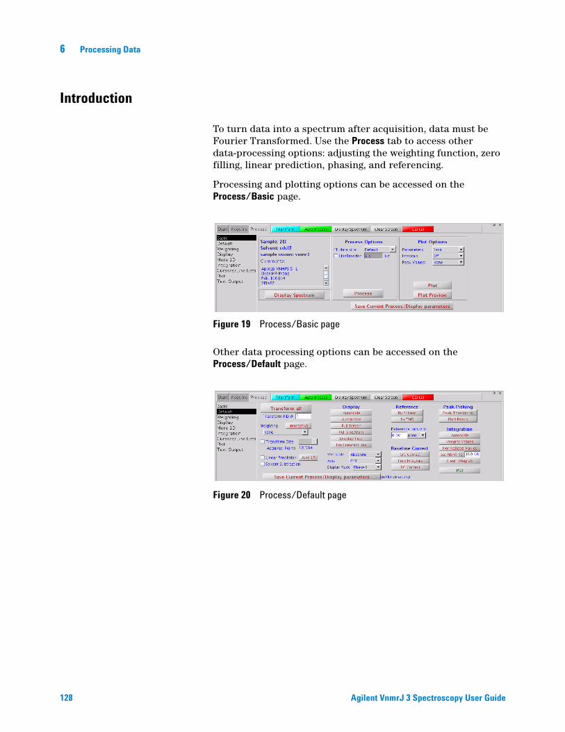
6 Processing Data
Introduction
128
To turn data into a spectrum after acquisition, data must be Fourier Transformed. Use the Process tab to access other data-processing options: adjusting the weighting function, zero filling, linear prediction, phasing, and referencing.
Processing and plotting options can be accessed on the Process/Basic page.
Other data processing options can be accessed on the Process/Default page.
Figure 19 Process/Basic page
Figure 20 Process/Default page
Agilent VnmrJ 3 Spectroscopy User Guide

Processing Data 6
Weighting Function
Agilent VnmrJ 3 Spectroscopy User Gui
The Process/Weighting page contains a full set of weighting-function action buttons. These automatically set the Weight parameters in the following way:
• exponential – A positive value gives the desired line broadening in Hz. This is also called a decaying exponential function. A negative value gives a resolution enhancement function. The parameter name is lb.
• gaussian – Time constant, in seconds, that defines a Gaussian function of the form exp(-(t/gf)2).
• shift – shifts the center of the Gaussian function exp(-((t-gfs)/gf)2).
• sine – A positive value, in seconds, applies a sinebell of the form sin(t*p/(2*sb)). A negative value applies a squared sinebell function of the form sin2(t*p/(2*sb)).
• shift – a sinebell shift constant, in seconds. It allows shifting the origin of the sinebell function according to the formula sin((t-sbs)*p/(2*sb)). Again, the square of this function is applied if sb is negative.
• additive Offset – An additive weighting constant that adds the constant awc to each value of the weighting function. It is applied after the sinebell and exponential function but before the Gaussian function.
As part of the Transform process, all weighting functions are set and applied simultaneously. Deselect the associated check box to remove a particular weighting function from use.
Figure 21 Process/Weighting page
de 129

130
6 Processing Data
The effects of combining sinebell, exponential, and Gaussian weighting can be complicated and should only be used after experimenting with the individual parameters. The use of either Gaussian apodization (which leads to Gaussian line shapes) or line broadening (values greater than 0 lead to Lorentzian lineshapes) is especially critical for deconvolution.
Other line shapes cannot be handled by the deconvolution program, but may be appropriate for 1D resolution enhancement or for absolute-value 2D experiments. Weighting functions (other than exponential) can alter the relative areas of the resonances within a spectrum, and so they should be used with great care if quantitative results are required.
The res-enhance button sets defaults of a equal to 0.1 and b equal to 0.3 into the formulas lb=-0.318/(a*sw), and gf=b*sw, thereby calculating “reasonable” values for the resolution enhancement parameters lb and gf. The arguments a and b can also be selected by the user.
Several macros exist that set weighting parameters to give certain window functions. These include gaussian, pi3ssbsq, pi4ssbsq, sqcosin, and sqsinebell.
The parameter wtfile is available for handling user-written weighting functions; see the manual VnmrJ 3 User Programming for details.
Agilent VnmrJ 3 Spectroscopy User Guide

Processing Data 6
Interactive Weighting
Agilent VnmrJ 3 Spectroscopy User Gui
Click the Interactive Weighting button on the Process panel to start interactive weighting.
Figure 22 The graphics display for interactive weightingde 131

132
6 Processing Data
Buttons next to the Interactive Weighting display provide access to the following functions:
Currently active weighting parameters can be changed by moving the cursor to the appropriate field in the weighting function box and pressing the left mouse button. New values for weighting parameters can also be typed in. Note that all other parameters, unless set to “not used”, are also used to calculate the weighting function.
Use the center mouse button within the FID box to adjust FID intensity (parameter vf). Use the center mouse button within the spectrum box to adjust spectrum intensity (vs). Use the right mouse button to turn the display of the transformed spectrum off and on. (It will be off by default whenever fn > 25000.)
Check box Icon Function
Line broadening Selects line broadening or exponential weighting. A negative value gives resolution enhancement.
Sinebell Selects the sinebell constant. A negative value gives squared sinebell. Change sign by clicking outside the box at the left.
Shifted Sinebell Selects the sinebell shift constant (if sinebell is active).
Gaussian Selects the Gaussian time constant.
Shifted Gaussian Selects the Gaussian shift constant (if Gaussian is active).
Additive weighting Selects the additive weighting constant.
Return Returns to the previous menu.
Agilent VnmrJ 3 Spectroscopy User Guide

Processing Data 6
Fourier Transformation
Agilent VnmrJ 3 Spectroscopy User Gui
The Transform all button will Fourier transform one or more FIDs. It uses the Transform Size parameters, and weighting functions are simultaneously applied whenever any weighting options are selected. Other options listed on the More 1D page are also simultaneously applied (such as Linear Prediction, Solvent Subtraction, FID Shift, and FID phase rotation). The data processing options Baseline Correct and Drift Correct are only applied as separate discrete actions that are used after the Fourier Transform.
The Transform Size field is the number of points to be Fourier transformed (fn), and the number must be a power of two; typical numbers are 16384, 32768, or 65536 (listed as 16K, 32K, and 64K, where K is a multiplier of 1024). The most common entry for Transform Size is Default. This value specifies that however many data points (np) were acquired, the first power of two greater than or equal to np will be used as fn. If fn is greater than np, or if fn is 'n' and np is not a power of two, the remaining points in the transform are filled in with values of zero (zero-filling). (If np is <10% bigger than fn, the software will round down instead of up.) Thus, there is no explicit zero-filling command. This process is an implicit one governed by the relationship between fn and np. The number of complex data points is fn/2.
de 133
6 Processing Data
Phasing
134
Phasing spectra may be considered part of either data processing or data display. Performing a complex Fourier transformation produces two sets of data, referred to as the cosine and sine transforms, or the real and imaginary data sets, respectively. The absorption spectrum (peaks “in-phase”) and the dispersion spectrum (peaks “out-of-phase”) generally do not coincide with either the real or the imaginary channels, but must instead be produced from a linear combination of the two spectra.
Phasing can be adjusted using Phase button for interactive phasing or using the Autophase functions on the Process/Default page.
Phase parameters
The process of phasing a spectrum requires the determination of an angle θ that can be used to “mix” these two data sets to produce one data set, according to the formula:
The process is complicated by the fact that the phase angle θ is a function of frequency:
where lp (left or first-order phase) and rp (right or zero-order phase) are constants that must be determined.
The following is clear about the terms in Equation 2:
• rp is frequency independent. Changes in rp affect all peaks in the spectrum equally.
• lp is frequency dependent. Changes in lp affect peaks with a differing amount as a function of frequency.
There are several ways in which lp and rp can be adjusted:
• Like any parameter, they can be recalled with a particular parameter set. They can also be entered directly (for example, lp=150).
Absorption spectrum =real* cosθ + imaginary* sinθ [Eq. 1]
θ = rp + (w-w0) /sw*lp [Eq. 2]
Agilent VnmrJ 3 Spectroscopy User Guide
Processing Data 6
Agilent VnmrJ 3 Spectroscopy User Gui
• Fully automatic phasing is also provided with the aph and aph0 commands. The aph command optimizes both the frequency-dependent (lp) and the frequency-independent (rp) parameters, and is independent of the starting point. The aph0 command adjusts only rp. The aphx macro optimizes parameters and arguments for the aph command. aphx first performs an aph then calculates a theoretical value for lp. If lp set by the aph is different from the calculated value by 10 percent, the calculated value is used and an aph0 is performed.
The command phase (phase_change) changes the phase of all peaks in the spectrum by adding phase_change to the current value of rp, and can remove any excess in rp more than 360°.
Autophase algorithm
The automatic phasing algorithms aph and aph0 have the following features:
• Weighting parameters do not affect the algorithms.
• Spectra with very low signal-to-noise can be phased.
• In vivo spectra can be phased, which is very difficult for most autophasing algorithms.
• Spectra with inverted lines can be phased. Such spectra include APT or DEPT data or selectively inverted lines obtained with shaped pulses. This type of phasing is difficult for traditional autophasing algorithms.
The autophasing algorithm uses many rules that are used in a manual phasing procedure. First, it finds the peak areas. Then, it estimates the correct phase for each peak. An initial guess of the first-order phasing parameter lp is made based upon the estimated phases of two “normal” peaks. The peaks are categorized into three classes: normal, inverted, and bad. The peaks in the normal and inverted group will be used to find the optimal values for the phasing parameters lp and rp. A final check is made to determine whether autophasing was successful or unsuccessful.
Algorithms are complicated but fairly “intelligent.” The key point of an algorithm is to use a set of fuzzy rules to estimate the correct phase for each peak. The use of these rules makes an algorithm less sensitive to the signal-to-noise ratio, the weighting parameters, and the baseline quality. Fuzzy logic also makes it possible to do the classifications on the peaks.
The command aphb autophases Bruker data. See the Command and Parameter Reference for more information about this command.
de 135

6 Processing Data
Spectrum display
136
The displayed spectrum is calculated in one of the following four mutually exclusive modes. The first three can be selected by radio buttons in the Process/Display page.
• The phase-sensitive mode is selected by the command ph. In this mode, the displayed spectrum is calculated using the phase parameters lp and rp. This is the most commonly used mode.
• The absolute-value mode is selected by the command av. In this mode, the displayed spectrum is calculated according to the equation
• absorption spectrum(ω) = (real2 (ω) + imaginary2(ω)1/2
• The power mode is selected by the command pwr. In this mode, the displayed spectrum is the square of the displayed spectrum calculated in the absolute value mode.
• The phase-angle mode is selected by the command pa. In this mode, each point in the displayed spectrum is the arc-tangent of the phase angle of the real and imaginary point.
Once a spectrum is displayed using the interactive display command ds, the spectrum can be interactively phased by selecting the Phase button from the graphical tool bar. When the spectrum is in the Phase mode, the integral and cursors are not displayed.
Figure 23 Process/Display page
Agilent VnmrJ 3 Spectroscopy User Guide

Processing Data 6
Advanced Data Processing
Agilent VnmrJ 3 Spectroscopy User Gui
This section covers the functions available on the More 1D page: advanced data processing, including linear prediction, FID shifting, FID phase rotation, and frequency shifting.
FID manipulation
Check Box Function
1st Pt Multiplier Allows correction of the first point of the FID if it is distorted. See the fpmult parameter in the VnmrJ 3 Command and Parameter Reference.
FID Phase Rotation The parameter phfid is a zero-order FID phasing constant. If phfid is set to a value other than 'n', the FID is phase-rotated by phfid degrees before weighting or Fourier transformation is performed.
Left Shift FID The parameter lsfid is a constant used in left-shifting the FID. If lsfid is set to a value other than 'n', the FID is left-shifted by lsfid complex points before weighting or Fourier transformation is performed. The value for lsfid must lie between 0 and np/2.
The tmove macro provides a graphical method of setting the parameter lsfid—position the left cursor at the place that should be the start of the FID, then enter tmove to adjust the parameter lsfid.
Left Shift Frequency Sets the frequency shift of spectral data, in Hz. See lsfrq in the VnmrJ 3 Command and Parameter Reference.
Sets a frequency shift of spectral data, in Hz, with a negative value resulting in peaks being shifted upfield (to the right) and a positive value in peaks being shifted downfield (to the left). lsfrq operates in the time domain on complex FID data, and so the desired value must be entered prior to Fourier transformation.
de 137

6 Processing Data
Data processing methods
138
All data processed in VnmrJ 3 are processed by using the Fourier transform, but there are three variations, which are governed by the proc parameter:
• Two orthogonal (real and imaginary, or x and y) data points are sampled at the same time and form a single complex data point in the FID. Such data are processed using a normal complex Fourier transformation, using proc='ft'.
• Some spectrometers (Bruker Instruments) acquire pseudo-quadrature data by sampling two orthogonal data points sequentially, rather than simultaneously. Such data must be processed using a real Fourier transformation, with proc='rft'.
• For complex data only, it is possible to include “linear prediction,” as part of the data processing. proc='lp' is used to trigger this operation.
Linear prediction
Use the Linear Prediction page to control linear prediction and to adjust its parameters.
Linear Prediction in VnmrJ 3
Linear prediction is incorporated into the Fourier transform routine, so that you do not normally see the “improved” FID, but merely the resulting spectrum (which results from Fourier transforming the linear predicted FID). This is accomplished by selecting the Linear Prediction check box in the Linear Prediction panel and clicking on the Transform button.
Agilent VnmrJ 3 Spectroscopy User Guide

Processing Data 6
Agilent VnmrJ 3 Spectroscopy User Gui
Enter ft('noft') to suppress display of the linear-predicted spectrum and perform all the steps of the Fourier transform routine except the actual Fourier transformation. Real points of the FID are displayed by setting lp=0 rp=0, or display the imaginary points by setting lp=0 rp=90.
Linear prediction involves solving a series of equations for appropriate coefficients based on the actual FID. It involves quite a number of parameters and can be somewhat tricky to optimize (if not optimized properly, or if the data are not amenable, the analysis may simply fail, just like any least-squares fit process may fail to converge).
Linear prediction can be run in an iterative fashion by arranging the LP parameters—first extending backward, then forward, and backward again for more complex problems.
Why Use Linear Prediction?
Raw time-domain data acquired during a pulsed NMR experiment can have two flaws:
• Early points in the FID may be distorted due to a host of hardware characteristics, such as preamplifier saturation and probe ringing. Even on a perfect spectrometer, these distortions cannot always be avoided.
• The acquisition time of each FID may have been too short to allow for full decay of the signal, leading to distortion in the Fourier transformed spectrum.
Both types of distortions can be solved using linear prediction. This uses the “good” part of the FID to analyze for the frequencies that are present in the signal, and then uses that information to extend the FID either in a reverse direction (to “fix” the first few “bad” points) or in a forward direction (to eliminate truncation problems, or even single “bad” points). Following this process, the “new, improved” FID is then Fourier transformed in the usual way.
See H. Barkhuijsen, R. de Beer, W.M.M.J. Bovee, and D. van Ormondt, J. Magn. Reson., 61, 465-481 (1985) for more information on the algorithm implemented in the software, and on linear prediction in general.
de 139

6 Processing Data
Solvent subtraction filtering
140
Numerous solvent suppression pulse sequences exist that reduce the signal from a large solvent peak to a level where the desired resonances can be observed. Often, however, experimental solvent suppression does not entirely eliminate an unwanted solvent peak. Digital filtering of the data can further suppress or eliminate a solvent peak.
VnmrJ 3 incorporates two algorithms for solvent subtraction by digital filtering:
• bandwidth — Sets the value of ssfilter to specify the full bandwidth of the low-pass filter applied to the original FID to yield a filtered FID. Its default value is 100 Hz.
• coefs. — Sets the value of ssntaps to specify the number of taps (coefficients) used for the digital filter. The default value is 121, but the value can range from 1 to np/4. The more taps in a filter, the flatter the passband response and the steeper the transition from passband to stopband, giving a more rectangular filter. An increased number of taps also increases the computational time dramatically (so that it might become noticeable). The default is suitable for low-frequency suppression option. A value between 3 and 21 works better for the zero-frequency suppression option.
• polynomial — Sets the value of ssorder to determine the polynomial used to create a low-pass filter applied to the FID acquired with the solvent on resonance. The resulting FID is subtracted from the original FID to remove the on-resonance frequencies. Transforming the resulting FID produces a solvent-subtracted spectrum. Another name for this is zero-frequency suppression.
Agilent VnmrJ 3 Spectroscopy User Guide

Processing Data 6
Agilent VnmrJ 3 Spectroscopy User Gui
• offset — Sets the value of sslsfrq, which adjusts the location of the solvent-suppressed region of the spectrum. Setting sslsfrq to a non-zero value shifts the solvent-suppressed region by sslsfrq Hz. Setting sslsfrq to 'n' (the default value) solvent suppresses a region centered about the transmitter frequency. The parameters may be arrayed to achieve multiple-frequency suppression. The quality of zero-frequency suppression diminishes rapidly as the solvent peak moves off the exact center of the digital filter. Adjust sslsfrq to move the center of the filter to within ± 0.2 Hz of the solvent peak for optimal solvent suppression.
Downsample
User-controlled downsampling is not routinely needed on data acquired on newer consoles, but it can be used on virtually all NMR data if desired.
• divide by — Sets the value of the downsampling factor thatwill be applied after digital filtering. The spectral width of the data set after digital filtering and downsampling is sw divided by downsamp, where sw is the acquired spectral width.
• coefs — Sets the value of dscoef to specify the number of coefficients used in the digital filter. This parameter is automatically adjusted by VnmrJ 3 to give filter cutoffs that are the same value of downsamp by using dscoef*downsamp/2 coefficients in the digital filter. VnmrJ 3 always rounds dscoef*downsamp/2 to an odd number. The default is 61.
de 141

142
6 Processing Data
• offset — Sets the value of a bandpass filter, in Hz, that is not centered about the transmitter frequency. A positive value selects a region upfield from the transmitter frequency; a negative value selects a downfield region.
Interleave FIDs
The ilfid command converts a multiple FID element into a single FID by interleaving the FIDs. When invoked in an experiment of nf FIDs, each of np points, ilfid sorts the data into a single FID of np*nf points that can then be transformed. The interleaving takes the first complex point of each of the nf FIDs and places them in sequential order in the new FID. It then takes the second complex point from each of the nf FIDs and appends them sequentially to the new FID. This operation is repeated for all complex points. Although ilfid adjusts np and nf, it does not alter other parameters such as sw. See the VnmrJ 3 Command and Parameter Reference for further information on ilfid, including an example.
CAUTION Because ilfid alters the data irrevocably, it is strongly recommended to save the FID before using ilfid.
Agilent VnmrJ 3 Spectroscopy User Guide

Agilent VnmrJ 3 SpectroscopyUser Guide
7Displaying FIDs and Spectra
Displaying a FID or 1D Spectrum 144
Display Tools 146
Graphics Control Buttons 150
Phasing 153
Line Tools 156
Spectral Referencing 157
Display an Inset Spectrum Using Viewport Tab 159
Stacked 1D Display 165
Aligning and Stacking Spectra 168
Integration 171
Molecular Display and Editing (JChemPaint and Jmol) 179
143Agilent Technologies

7 Displaying FIDs and Spectra
Displaying a FID or 1D Spectrum
144
Click the Display FID graphics control button to display a FID. Click the 1D Spectrum graphics control button to display a 1D spectrum.
FID display
An FID is available for displaying upon completion of the
acquisition of acquisition block size. Clicking the FID icon
displays a FID and enables interactive manipulation of the FID display.
The FID display graphics buttons change to show that multiple FIDs can be viewed. Figure 24 shows a typical display with a FID and two vertical cursors (box mode).
The FID is also phase-rotated (zero-order only) by the number of degrees specified in the FID Phase Rotation field on the Linear Prediction page.
1D spectrum display
After data is transformed, a spectrum becomes available for display and plotting.
The normal spectrum display enables interactive manipulation of a single 1D spectrum. A spectrum is displayed by clicking on
the 1D Spectrum graphics control icon or by transforming a
data set.
Figure 24 Interactive FID display
Agilent VnmrJ 3 Spectroscopy User Guide
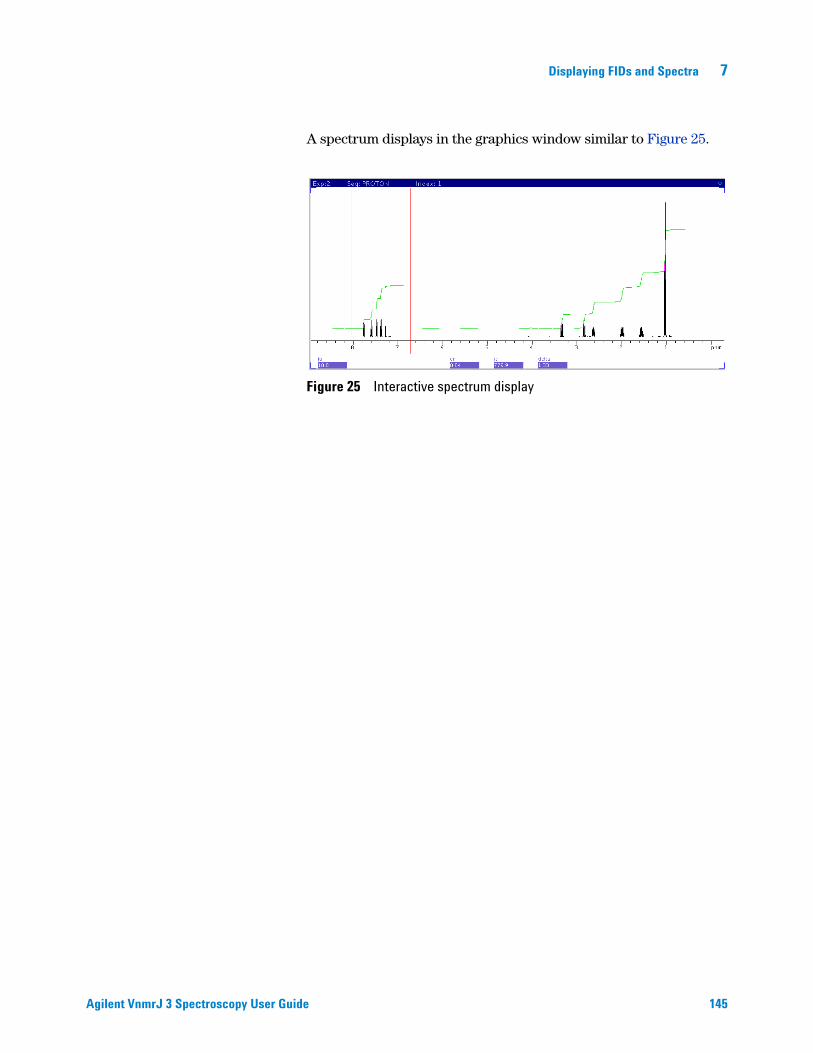
Displaying FIDs and Spectra 7
Agilent VnmrJ 3 Spectroscopy User Gui
A spectrum displays in the graphics window similar to Figure 25.
Figure 25 Interactive spectrum display
de 145

7 Displaying FIDs and Spectra
Display Tools
146
VnmrJ 3 provides interactive tools for creating individualized displays of NMR data.
Interactive display tools
These tools are described below:
A typical use of these tools might be to expand a region on a spectrum:
1 Display the spectrum – click the spectrum icon on the graphics control bar.
2 Select the region to expand – left click the spectrum to place the cursor on the left boundary of the region of interest, and right-click to designate the right boundary. Use the left mouse button to drag the left cursor and right button to drag the right cursor until the desired region is between the cursors.
3 Expand the region – click the magnifying glass icon on the graphics control bar.
Mouse buttons The mouse buttons correspond to the display parameters shown on the lower right part of the graphics window. The display parameter changes as different graphics control functions are selected. Typically, the left button controls the left cursor position, the middle button controls vertical scaling, and the right button controls the right cursor or delta between the two cursors.
Graphics control buttons
The graphics control bar next to the graphics canvas provides graphics control buttons for cursors, zooming, scales, grab and move, threshold, phasing, and refresh. Different functions appear for FID or spectrum display.
Display page The Display page on the Process tab provides appropriate display parameters, including display mode, axis, and amplitude scaling.
Display menu The Display menu provides tools for displaying multiple spectra, plotting, and creating insets.
Agilent VnmrJ 3 Spectroscopy User Guide

Displaying FIDs and Spectra 7
Display parameters
Agilent VnmrJ 3 Spectroscopy User Gui
FID and spectral display is governed by parameters on the Display page.
Display Mode
The Display Mode parameters set the display mode along the directly or indirectly detected dimension.
Axis
The Axis parameters set the labeling of plot scales, peak frequencies, etc. Typically, FID display is in seconds, and spectrum display is in PPM, Hz, or kHz.
Phased Each real point in the displayed spectrum is calculated from a linear combination of real and imaginary points comprising each respective complex data point.
Absval (Absolute value mode) Each real point in the displayed spectrum is calculated as a square root of the sum of squares of the real and imaginary points comprising each respective complex data point.
Power Each real point in the displayed spectrum is calculated as a sum of squares of real and imaginary points comprising each respective complex data point.
de 147

148
7 Displaying FIDs and Spectra
Amplitude scaling
The amplitude scaling, or vertical scale, parameters set the scale intensities for the display:
For vertical scaling, full scale on the screen represents full scale on the plotter. This relationship is used to adjust the vertical scale in the Absolute display mode, because vertical scale is not the height of the largest peak. Use the Normalized amplitude scaling mode when the largest peak is to be off-scale.
An exception to the general rule of plotting is provided by the wysiwyg parameter. This parameter is set in the Edit > System settings window, on the Display/Plot tab: Set display from plotter aspect ratio (wysiwyg).
Screen position
The screen position parameters set the horizontal position of the display on the screen and the plotter. Clicking one of the buttons updates the display:
Normalized The largest peak in the spectrum is automatically found, then the display is normalized to make the peak vertical scale on the plot in millimeters.
Absolute The appearance on the display screen is used as a guide to adjust the vertical scale to produce the desired height. This mode enables comparing intensity from one experiment to another, a necessity for all arrayed experiments.
Checked Scales the image to the current plotter setting (wysiwyg).
Unchecked Scales the image to the full window, which is easier to view. This option scales the window but does not change the ratio of the image.
Full Display or plot on the entire screen or page.
Center Display or plot in the center of the screen or page.
Left Display or plot in the left half of the screen or page.
Right Display or plot in the right portion of the screen or page.
Agilent VnmrJ 3 Spectroscopy User Guide

Displaying FIDs and Spectra 7
Controlling cursors and vertical scale
Agilent VnmrJ 3 Spectroscopy User Gui
Click the mouse buttons in the graphics display window to position cursors and adjust the FID or spectral vertical scale and position.
Left cursor Click the left mouse button to position the cursor and update the value displayed for the crf or cr parameter (crf for a FID or cr for a spectrum).
Right cursor (box) Click the right mouse button to display and position a second cursor to the right of the original cursor. The value of the parameter deltaf for a FID or delta for a spectra changes with the position of the right cursor and is the difference in seconds or Hz between the two cursors.
Two cursors If both cursors are displayed, the left mouse button moves both cursors simultaneously, leaving the distance between them (deltaf or delta) unchanged.
Vertical scale Click the middle mouse button to adjust the vertical scale of the FID (vf parameter) or spectrum (vs parameter).
Vertical position Adjust the vertical position of the FID by clicking and holding the middle mouse button near the left edge of the graphics display and sliding the FID or spectrum up or down. The value of vpf or vp (or vpfi if the imaginary channel) is will change.
Display limits
The screen position buttons (Full, Enter, Left, Right) on the Display page place the display and plot in the desired portion of the page.
The wysiwyg parameter is useful for scaling the image to a full window instead of the same size as the plot. This parameter is set in the Edit > System settings window, on the Display/Plot tab: Set display from plotter aspect ratio (wysiwyg).
Checked Scales the image to the current plotter setting (wysiwyg).
Unchecked Scales the image to the full window, which is easier to view. This option scales the window but does not change the ratio of the image.
de 149
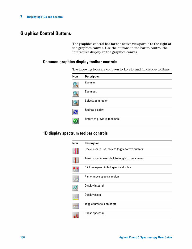
7 Displaying FIDs and Spectra
Graphics Control Buttons
150
The graphics control bar for the active viewport is to the right of the graphics canvas. Use the buttons in the bar to control the interactive display in the graphics canvas.
Common graphics display toolbar controls
The following tools are common to 1D, nD, and fid display toolbars.
Icon Description
Zoom in
Zoom out
Select zoom region
Redraw display
Return to previous tool menu
1D display spectrum toolbar controls
Icon Description
One cursor in use, click to toggle to two cursors
Two cursors in use, click to toggle to one cursor
Click to expand to full spectral display
Pan or move spectral region
Display integral
Display scale
Toggle threshold on or off
Phase spectrum
Agilent VnmrJ 3 Spectroscopy User Guide

Displaying FIDs and Spectra 7
Display FID toolbar controls
Agilent VnmrJ 3 Spectroscopy User Gui
Icon Description
One cursor in use, click to toggle to two cursor
Two cursors in use, click to toggle to one cursor
Click to expand to full FID display
Pan and stretch
Click to show real and imaginary
Click to show real and zero imaginary
Click to show real only
Toggle scale on and off
Phase FID
Main nD Display Bar Tools
Icon Description
Display color map and show common nD graphics tools
Display contour map and show common nD graphics tools
Display stacked spectra and show common nD graphics tools
Display image map and show common nD graphics tools
de 151
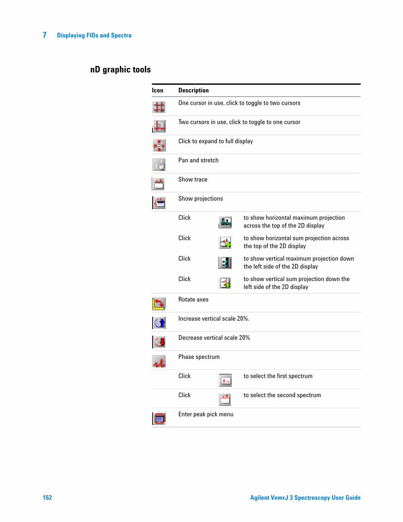
7 Displaying FIDs and Spectra
nD graphic tools
152
Icon Description
One cursor in use, click to toggle to two cursors
Two cursors in use, click to toggle to one cursor
Click to expand to full display
Pan and stretch
Show trace
Show projections
Click to show horizontal maximum projection across the top of the 2D display
Click to show horizontal sum projection across the top of the 2D display
Click to show vertical maximum projection down the left side of the 2D display
Click to show vertical sum projection down the left side of the 2D display
Rotate axes
Increase vertical scale 20%.
Decrease vertical scale 20%
Phase spectrum
Click to select the first spectrum
Click to select the second spectrum
Enter peak pick menu
Agilent VnmrJ 3 Spectroscopy User Guide

Displaying FIDs and Spectra 7
Phasing
Agilent VnmrJ 3 Spectroscopy User Gui
The Phase button starts the interactive phasing mode. Any integral and cursors that are displayed along with the spectrum are removed. The width of the update region is set by the Spectrum updating during phasing (0-100) field in Edit > System settings > Display/Plot tab, which sets the percentage of the screen display to be updated.
FID phasing
The Phase button activates the interactive phasing mode:
1 Position the mouse arrow on a FID region of interest, about halfway vertically up the screen, and click the left mouse button.
A horizontal cursor intersects at the mouse arrow, and two vertical cursors are placed on either side of the mouse arrow. A small region of the FID is displayed in a different color if a color display is present. Only this spectral region is interactively updated.
2 Move the mouse above or below the horizontal cursor, but within the two vertical cursors. Click the left or right button to adjust the FID phase parameter phfid.
Click the mouse above the horizontal cursor to increase phfid. Click below the horizontal cursor to decrease phfid. Place the mouse arrow right on the horizontal cursor and click the left button to restore the initial phase.
3 To exit the interactive phasing mode, make another selection from the menu. Select the Cursor or Box button if no other choice is desirable.
de 153

7 Displaying FIDs and Spectra
Spectrum phasing
154
1 Position the mouse arrow on a spectral region of interest toward the right side of the spectrum, about halfway vertically up the screen, and click the left mouse button.
A horizontal cursor will intersect at the mouse arrow. Two vertical cursors will be placed on either side of the mouse arrow. A region of the spectrum will be displayed in a different color if a color display is present, and only this spectral region will be interactively updated (for the case of less than 100% updating).
2 Move the mouse above or below the horizontal cursor, but within the two vertical cursors. Click the left or right button to adjust the zero-order or frequency-independent phase parameter rp.
• Click above the horizontal cursor to increase rp (cause a clockwise rotation of the peaks).
• Click below the horizontal cursor to decrease rp (and cause a counter-clockwise rotation).
• Place the arrow on the horizontal cursor and click the left button to restore the initial phase.
The left and right buttons of the mouse differ only in their sensitivity. Full scale (top to bottom of the screen) corresponds to approximately 180° for the left button, and 20° for the right button. The left button is a “coarser” adjustment, and the right button is a “finer” adjustment.
3 Move the mouse arrow to another region of the spectrum, near the left edge of the display, outside the vertical cursors, and click the left mouse button again.
The frequency-independent phase-correction made so far is first applied to the entire spectrum. A new horizontal cursor is displayed at the mouse arrow, and two new vertical cursors are displayed on either side of the mouse arrows. The mouse now controls the first-order or frequency-dependent phase parameter lp.
4 Click the left or right button above or below the horizontal cursor to increase or decrease lp so that the phase at the center of the previous region bracketed by the vertical cursors is held constant.
This process eliminates or substantially reduces the necessity to iteratively adjust the two parameters rp and lp. As with the zero-order correction, the left button acts as a “coarse” adjust, and the right button as a “fine.”
Agilent VnmrJ 3 Spectroscopy User Guide

Displaying FIDs and Spectra 7
Agilent VnmrJ 3 Spectroscopy User Gui
Define a new update region by clicking the mouse outside the two vertical cursors.
Subsequent first-order phase changes cause the zero-order phase to be adjusted so that the phase angle at the center of the previous region bracketed by the vertical cursors remains constant. Click the Phase button again if to return to the zero-order phase correction.
Adjust the vertical scale and apply the latest phase correction by clicking the middle mouse button at the top of a peak that is on scale. This leaves the vertical scale unaffected but recalculates the phase of the entire spectrum. Clicking the center button above or below the peak raises or lowers the vertical scale.
5 Exit the interactive phasing mode by clicking another graphics control button.
de 155

7 Displaying FIDs and Spectra
Line Tools
Find nearest line and line resolution
156
1 Place a cursor near the line of interest.
2 Select the Process page and click the Find nearest line button. The cursor moves to the nearest line and displays its height and frequency (in Hz and ppm) in the message window.
3 Click Display linewidth to display the resolution of a line, as well as the limiting digital resolution of the spectrum. The resolution is determined by a width at half-height algorithm and not by least-squares.
Display line list
1 Click the Threshold graphics control button and use the middle mouse button to vertically position the yellow threshold line.
2 Select the Line List page and click the Display Line List button. This process displays line frequencies and intensities that are above a threshold.
Agilent VnmrJ 3 Spectroscopy User Guide

Displaying FIDs and Spectra 7
Spectral Referencing
Agilent VnmrJ 3 Spectroscopy User Gui
Frequency referencing is set on the Display page.
Button Description
By Solvent Reference the spectrum for selected solvent.
By TMS Reference the spectrum to a TMS line. In the case of other signals (for example, from silicon grease) immediately to the left of the TMS line (even if they are higher than the reference line), tmsref tries avoiding those signals by taking the line furthest to the right in that area, as long as it is at least 10% of the main Si-CH3 signal. Large signals within 0.6 ppm for 1H (or 6 ppm for 13C) to the right of TMS might lead to mis-referencing.
Cancel Clears the reference line by removing any spectral referencing present, and turns off referencing.
By Cursor References the spectrum based on the current cursor position. To reference the spectrum based on a line position in the spectrum, first use the Find nearest line button on the Process page, then click By Cursor.
Table 7 Parameters used in spectral referencing
Reference line (frl) The distance, in Hz, of the reference line from the right edge of the spectral window. This line is the spectral position used to set the referencing. It can be the signal of a frequency standard (such as TMS), or any line (such as a solvent signal) with a known chemical shift (in ppm), or a position in the spectrum where such a line is expected to appear.
de 157

158
7 Displaying FIDs and Spectra
The By Solvent and By TMS buttons assume that the system is locked (and that the lock solvent is defined in /vnmr/solvents). Ensure that the field offset has been adjusted so that the lock frequency is on resonance with a sample of similar susceptibility if the experiment is to run unlocked and these buttons are used to set the field offset. Adjust the field offset is adjusted using the following procedure:
1 Insert a sample with deuterated solvent.
2 Adjust z0 (or lkof) in acqi so that the lock frequency is on resonance.
3 Switch off the lock.
4 Insert the non-deuterated sample.
The accuracy of the solvent and TMS referencing buttons is mostly limited by the accuracy of the chemical shift of the lock resonance line, which may depend on the concentration and the chemical properties (acidity/basicity) of the components in the sample. But they should normally be accurate enough to find an actual reference line close to its predicted position.
Estimate the position of the reference frequency in spectra from unlocked samples, provided the spectrometer is first locked on a sample with similar susceptibility, then the lock is disengaged and the field offset adjusted such that the lock signal is on-resonance. Now, acquire a spectra without lock and calculate their (estimated) referencing using setref, provided the solvent parameter is set to the solvent that was last locked on.
Reference position (rfp) The difference between the reference line and the reference frequency (zero position of the scale) in Hz. Referencing a spectrum using the signal of a frequency standard, such as TMS, use reference position is 0. The distance of the reference frequency from the right edge of the spectrum is reference line reference position.
Spectrometer frequency The absolute frequency, in MHz, of the center of the spectrum (the transmitter position). Use the spcfrq command in order to see the accurate value of the spectrometer frequency (sfrq parameter).
Reference frequency The frequency, in MHz, of the frequency standard, that is, the zero position of the frequency scale, and the divider (unit) for the calculation of ppm scales (reffreq).
Table 7 Parameters used in spectral referencing (continued)
Agilent VnmrJ 3 Spectroscopy User Guide

Displaying FIDs and Spectra 7
Display an Inset Spectrum Using Viewport Tab
Viewport tab
Agilent VnmrJ 3 Spectroscopy User Gui
Click the Viewport tab to display the viewport controls. If the tab is not visible, click View on the main menu and select Viewport.
Figure 26 Viewport tab and controls
de 159

7 Displaying FIDs and Spectra
Frame Tab
160
The Frame tab, see Figure 27, of the viewport tab has the following tools, button, and check boxes:
Figure 27 Frame tab and controls
Table 8 Viewport tools
Icon Function
Default mode — left mouse click moves the left cursor and right mouse click moves right mouse cursor.
Inset mode — left mouse drag a box over a spectrum region creates an inset frame of the region. A viewport can have multiple inset frames.Exit inset mode — release mouse button.
Agilent VnmrJ 3 Spectroscopy User Guide

Displaying FIDs and Spectra 7
Agilent VnmrJ 3 Spectroscopy User Gui
Inset frame buttons
The buttons delete one or all inset frames and restore the default frame to full size.
Display check boxes
The check boxes control optional display features.
Button Function
Delete Inset Delete the selected inset.
Delete all Delete all inset frames.
Full size Restore the default frame to its full size.
Check box Function
Cross hair Display cross hair and chemical shift(s) of the cursor position when the mouse is moved over the spectrum. A useful function when the fields are not shown, not in cursor mode (default mode), or when chemical shift of a peak without moving the left cursor is required while in the cursor mode.
Fields Display cr, delta, vp etc... fields at the bottom of the viewport.
Axis Show scale of the axis.
Show frame border Check the box to display a box around the frame. Un-check the box to display the four corners of the selected frame as hot spots for resizing. No border or corner will be displayed if a frame is not selected. An empty frame is not visible until it is selected.
de 161

7 Displaying FIDs and Spectra
Working with viewports and inset frames
162
All VnmrJ 3 graphics are displayed in frame(s). The viewport has a default frame that occupies the entire viewport graphics area. An inset frame initially shares the same workspace and data as the original frame and is manipulated in the same way as the default frame.
Creating an inset frame
An inset frame has the full capability of the default frame. The only difference is that the default always exists, while an inset frame can be created and removed. Create an inset frame within the default viewport frame as follows:
1 Select the inset mode tool .
2 Place the cursor at the low field (left) side of the region to be expanded as shown in Figure 28 frame 1a.
3 Hold the left mouse button down and drag the inset window to the high field (right) side of the region.
4 Drag the cursor down to set the height of the inset frame as shown in Figure 28 frame 1b.
5 Release the mouse button to create the inset frame, see Figure 28 frame 2.
Figure 28 Creating an inset frame
Agilent VnmrJ 3 Spectroscopy User Guide

Displaying FIDs and Spectra 7
Agilent VnmrJ 3 Spectroscopy User Gui
Zooming in on a region within an inset frame
1 Select the default mode tool .
2 Click inside the frame to make the frame active.
3 The frame has a yellow border when it is active and white border when it is inactive (these are the default colors of inactive and active frames).
4 Select the zoom mode tool .
5 Place the cursor at the low field (left) side of the region to be expanded as shown in Figure 28 frame 3a.
6 Hold the left mouse button down and drag the inset window to the high field (right) side of the region, Figure 28 frame 3b.
7 The region selected is indicated by a transparent gray rectangle.
8 Release the mouse button and the selected region expands to fill the inset box, Figure 28, frame 4.
Resizing an inset frame
1 Select the default mode tool .
2 Click inside the frame to make the frame active. An active frame has a yellow border.
3 Move the mouse cursor to a corner of the inset frame. The cursor changes from a single-headed arrow to a double-headed arrow.
4 Hold down the left mouse button and grab the corner of the frame.
5 Drag the corner to resize the frame.
6 Release the mouse button when the frame is at the desired size.
de 163

164
7 Displaying FIDs and Spectra
Moving an inset frame
1 Select the default mode tool .
2 Click inside the frame to make the frame active. An active frame has a yellow border.
3 Move the mouse cursor to an edge of the inset frame. The cursor changes from a single-headed arrow to a four-headed arrow.
4 Hold down the left mouse button and grab the edge of the frame.
5 Drag the frame to the new position.
6 Release the mouse button when the frame is at the desired position.
Agilent VnmrJ 3 Spectroscopy User Guide

Displaying FIDs and Spectra 7
Stacked 1D Display
Stacked display using the main menu display
Agilent VnmrJ 3 Spectroscopy User Gui
1 Click Display on the main menu.
2 Select a display mode from the drop-down menu:
• Display Multiple Spectra Horizontally
• Display Multiple Spectra w/ Labels
• Display Multiple Spectra Vertically
• Increase vertical Separation by 20%
• Decrease vertical Separation by 20%
• Create an Inset of the current Display
— Save Current Display Parameters
— Plot Current Display before Making Inset
— Make Inset
— Plot Inset and Return Original Display
Stacked display using the display page1 Click the Process tab.
2 Select the Display page.
de 165
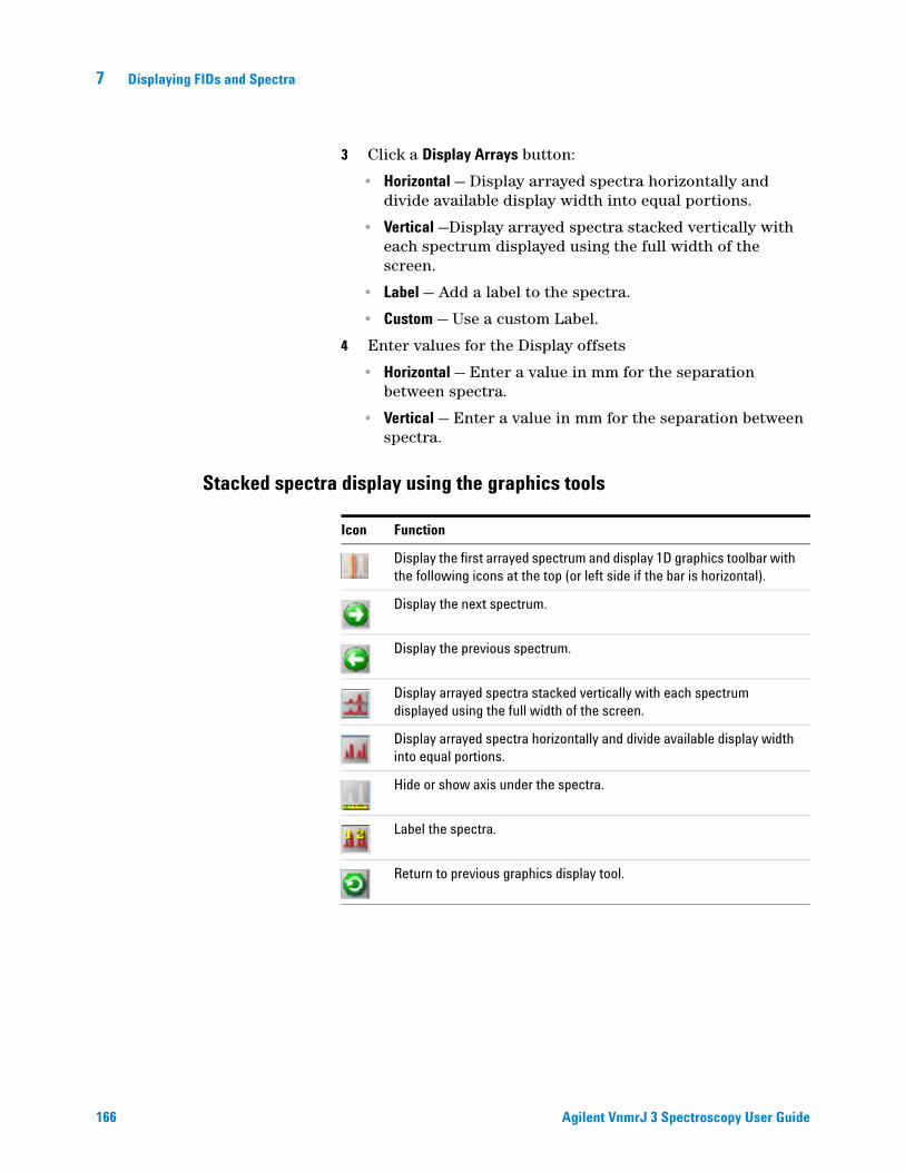
166
7 Displaying FIDs and Spectra
3 Click a Display Arrays button:
• Horizontal — Display arrayed spectra horizontally and divide available display width into equal portions.
• Vertical —Display arrayed spectra stacked vertically with each spectrum displayed using the full width of the screen.
• Label — Add a label to the spectra.
• Custom — Use a custom Label.
4 Enter values for the Display offsets
• Horizontal — Enter a value in mm for the separation between spectra.
• Vertical — Enter a value in mm for the separation between spectra.
Stacked spectra display using the graphics tools
Icon Function
Display the first arrayed spectrum and display 1D graphics toolbar with the following icons at the top (or left side if the bar is horizontal).
Display the next spectrum.
Display the previous spectrum.
Display arrayed spectra stacked vertically with each spectrum displayed using the full width of the screen.
Display arrayed spectra horizontally and divide available display width into equal portions.
Hide or show axis under the spectra.
Label the spectra.
Return to previous graphics display tool.
Agilent VnmrJ 3 Spectroscopy User Guide

Displaying FIDs and Spectra 7
Stacked FID Display Using the Graphics Tools
Agilent VnmrJ 3 Spectroscopy User Gui
Icon Function
Display the first arrayed FID and display 1D FID graphics tool bar with the following icons at the top (or left side if the bar is horizontal).
Display the next FID.
Display the previous FID.
Display arrayed FIDs stacked vertically with each spectrum displayed using the full width of the screen.
Display arrayed FIDs horizontally and divide available display width into equal portions.
Label the FIDs.
Return to previous graphics display tool.
de 167

7 Displaying FIDs and Spectra
Aligning and Stacking Spectra
Requirements for aligning and stacking spectra
168
Spectra can be a mixture of 1D and 2D data sets, all 2D data sets, or all 1 D data sets provided these requirements are met:
• All selected viewports need to use a common scale.
• Data in the viewports may have different nuclei, different spectrum width, or different spectral regions. The common scale is determined based on data in all selected viewports and determines whether alignment or stacking is possible. Overlaid and stacked spectra are drawn based on the common scales.
• Alignment is enabled if more than one axis in more than one viewport has the same axis (H1, C13 etc.).
• Stacking is enabled when data in all viewports have the same axis/axes.
Setting up stacked aligned spectra
1 Select the Viewport tab from the vertical tabs panel.
2 Load each data set into a different viewport and process the data. Data must meet the requirements mentioned in “Requirements for aligning and stacking spectra” .
3 Select viewports containing spectra to overlay by placing a check in the check box under select.
4 Click the Overlay Viewports button to overlay all selected viewports.
The Stack Spectrum button, Figure 29, is displayed below the Overlay Viewports button if all spectra have the same dimension (all 1D or all 2D) and all axis/axes (nuclei) match. Stacked spectra are aligned and each spectrum is shifted along x and y. The shift between spectra is specified by x and y offset in the entry fields below the Stack Spectrum button. Spectral axes are also synchronized to enable zoom and pan of the spectrum without losing the alignment.
Agilent VnmrJ 3 Spectroscopy User Guide

Displaying FIDs and Spectra 7
Agilent VnmrJ 3 Spectroscopy User Gui
The Align Spectra button, Figure 30, is available if it is a mix of 1D and 2D spectra when multiple spectra are overlaid. All 2D spectra must have matching axes. All 1D data must match one of the 2D axes. 1D spectra are aligned and displayed at the margins of the 2D spectrum. 1D spectrum will be rotated if necessary to align with the 2D spectrum. Zoom and pan are synchronized when the spectra are aligned.
Figure 29 1D stacked spectra
Figure 30 2D spectra with overlaid 1D’s
de 169

170
7 Displaying FIDs and Spectra
The Stacked Spectrum button for 2Ds, Figure 31, is displayed below Overlay Viewport if all 2D spectra axes and nuclei match. Spectral axes are synchronized to enable zoom and pan of the spectra without losing alignment.
Figure 31 Stacked overlaid 2D spectra
Agilent VnmrJ 3 Spectroscopy User Guide
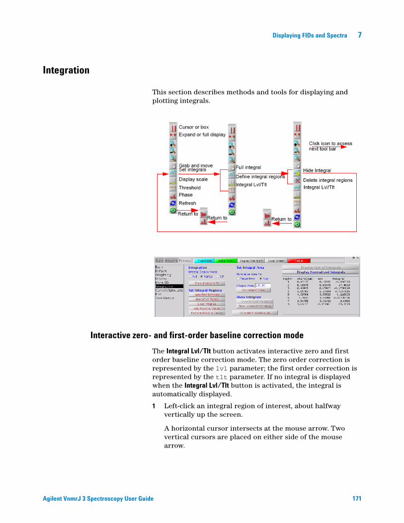
Displaying FIDs and Spectra 7
Integration
Agilent VnmrJ 3 Spectroscopy User Gui
This section describes methods and tools for displaying and plotting integrals.
Interactive zero- and first-order baseline correction mode
The Integral Lvl/Tlt button activates interactive zero and first order baseline correction mode. The zero order correction is represented by the lvl parameter; the first order correction is represented by the tlt parameter. If no integral is displayed when the Integral Lvl/Tlt button is activated, the integral is automatically displayed.
1 Left-click an integral region of interest, about halfway vertically up the screen.
A horizontal cursor intersects at the mouse arrow. Two vertical cursors are placed on either side of the mouse arrow.
de 171

172
7 Displaying FIDs and Spectra
2 Right or left-click above or below the horizontal cursor, but within the two vertical cursors, to adjust the zero-order baseline correction parameter lvl.
• Clicking above the horizontal cursor increases lvl.
• Clicking below the horizontal cursor decreases lvl.
• Clicking on the horizontal cursor restores the initial baseline correction value.
3 Left-click another region of the spectrum, outside the vertical cursors.
A new horizontal cursor is displayed at the mouse arrow, two new vertical cursors are displayed on either side of the mouse arrow, and a single vertical cursor is displayed in the middle of the region where lvl was being updated. The mouse now controls the first-order baseline correction parameter tlt.
4 Right or left-click above or below the horizontal cursor to increase or decrease tlt, and change lvl so that the total drift correction at the single vertical cursor in the middle of the previous region is held constant.
This process eliminates or substantially reduces the necessity to iteratively adjust the two parameters lvl and tlt. As with the zero-order correction, placing the mouse arrow right on the horizontal cursor and clicking the mouse button will restore the initial baseline correction values.
Each time the mouse is clicked outside the two vertical cursors, new vertical and horizontal cursors are displayed.
The left and right mouse buttons both adjust the baseline correction parameters and differ only in their sensitivity. The left button causes changes a factor of eight times larger than the right button, making the left button a “coarse” adjust and the right button a “fine” adjust. The overall sensitivity of these adjustments can also be controlled by the parameter lvltlt. This parameter is a multiplier, with a default value of 1.0, for the size of the changes. To make larger changes, make lvltlt larger than 1.0. To have finer control, set lvltlt to be between 0.0 and 1.0.
The middle mouse button adjusts the integral scale (parameter is) or the integral offset (parameter io), exactly as whenever an integral is displayed.
5 Exit the interactive baseline correction mode by clicking on another graphics control button.
Agilent VnmrJ 3 Spectroscopy User Guide

Displaying FIDs and Spectra 7
Displaying integrals step-by-step
Agilent VnmrJ 3 Spectroscopy User Gui
The following methods provide an opportunity to compare procedures. Before starting each procedure, be sure to obtain a typical spectrum.
1 Load a data file into the active viewport using the file browser or the Locator.
2 Transform the data if necessary.
3 Click the Process tab.
4 Select the Integration page.
5 Click an Integration Display Mode radio button: Full, Partial, or Off.
• Full shows integrals over the entire spectrum, including the noise.
• Partial shows even integrals regions and hides all the odd integral regions.
• Off turns off the integral display.
6 Click Auto Find Integrals to automatically set the integral resets and display the data as set by the Integration Display Mode radio button.
7 Click the Scale display to fit button to automatically scale the display.
8 Set the integral area.
9 Enter a value in the Integral Area field.
de 173

174
7 Displaying FIDs and Spectra
10 Click one of the following radio buttons under the Normalize Area to: page region.
• Single Peak — selects the region or peak under the cursor as the reference and sets the single peak integral to the value in the Integral Area field when the Set Integral Value button is clicked.
• Sum — sets the entire integral to the value in the Integral Area field. Do not click the Set Integral Value button. This button sets the single peak reference.
11 Display the integral results as follows:
• Single Peak — both the Show Integral Values and Show Normalized Value buttons are active.
• Integral Values Click Show Integral Values to display the values of the integral regions on the screen below the spectrum. Click Display Lists of Integrals to list the display regions and the value of the integral over each region.
• Normalized Integral Values Click Show Normalized Values to display the values of the integral regions normalized to the reference region on the screen below the spectrum. Click Display Normalized Integrals to list the display regions and the value of the integral over each region normalized to the reference region.
Manual method
1 Load a data file into the active viewport using the file browser or the Locator.
2 Transform the data if necessary.
3 Click the Process tab.
4 Select the Integration page.
5 Click Clear Integrals.
Any currently defined integral reset points are cleared.
Agilent VnmrJ 3 Spectroscopy User Guide

Displaying FIDs and Spectra 7
Agilent VnmrJ 3 Spectroscopy User Gui
6 Set up the integral resets from left to right (down field to up field).
a Click the Interactive Resets button.
b Place the cursor to the left of the first integral region.
c Click the left mouse button.
d Move the cursor to the right of the first integral region.
e Click the left mouse button.
f Repeat Step b through Step e until all the required integral regions are defined.
7 Click Scale display to fit button to automatically scale the display.
8 Set the integral area:
a Enter a value in the Integral Area field.
b Click one of the following radio buttons under the Normalize Area to: page region.
• Single Peak — selects the region or peak under the cursor as the reference and sets the single peak integral to the value in the Integral Area field when the Set Integral Value button is clicked.
• Sum — sets the entire integral to the value in the Integral Area field. Do not click the Set Integral Value button. This button sets the single peak reference.
9 Display the integral results as follows:
• Single Peak — both the Show Integral Values and Show Normalized Value buttons are active.
• Integral Values
Click Show Integral Values to display the values of the integral regions on the screen below the spectrum.
Click Display Lists of Integrals to list the display regions and the value of the integral over each region.
• Normalized Integral Values
Click Show Normalized Values to display the values of the integral regions normalized to the reference region on the screen below the spectrum.
Click Display Normalized Integrals to list the display regions and the value of the integral over each region normalized to the reference region.
de 175

7 Displaying FIDs and Spectra
Command line equivalents for vnmrj 3 interface driven integration
176
Use the parameter page editor to view the commands on the current parameter page.
1 Click Edit on the main menu.
2 Select Parameter Pages.
3 Place the mouse cursor on a button or entry field.
4 Double-click (left mouse button).
5 Read the associated command next to the field Vnmr Command.
Baseline correction
Most operations performed on spectra assume a quality baseline. Line lists, integrations, resolution measurements, 2D volume integrations, etc., all measure intensities from “zero” and do not perform any baseline adjustments. If the baseline in your spectrum is not flat perform a baseline correction operation before performing further data reduction. Two types of baseline correction are provided, linear and non-linear, and are available using the buttons on the Display page.
Baseline correction commands
Using the beginning and end of the displayed spectrum to define a straight line to be used for baseline correction, the dc command turns on a linear baseline correction. dc calculates a zero-order baseline correction parameter lvl and a first-order baseline correction parameter tlt. The cdc command turns off this correction. The results of the dc or cdc command are stored in the dcg parameter, which can be queried (dcg?) to determine whether drift correction is active. If active, dcg=''; if inactive, dcg='cdc'.
The bc command performs a 1D or 2D baseline correction. The 1D baseline correction uses spline or second to twentieth order polynomial fitting of predefined baseline regions. bc defines every other integral, that is, those integrals that disappear in partial integral mode (intmod='partial') as baseline and attempts to correct these points to zero. A variety of parameters can be used to control the effect of the bc command.
For more information about the bc command, see the entry for bc in the Command and Parameter Reference.
Agilent VnmrJ 3 Spectroscopy User Guide

Displaying FIDs and Spectra 7
Agilent VnmrJ 3 Spectroscopy User Gui
Integral reset points commands
The z command (or the equivalent button or icon) resets the integral to zero at the point marked by the displayed cursor. z(reset1,reset2,...) allows the input of the reset points as part of a command, instead of using the position of the cursor. Reset points do not have to be entered in order. The resets are stored as frequencies and will not change if the parameter fn is changed. The command cz (or the equivalent button) removes all such integral resets. cz(reset1,reset2,...) clears specific integral resets.
The liamp parameter stores the integral amplitudes at the integral resets points, and the lifrq parameter stores the frequencies of integral reset points, for a list of integrals. To display the values of liamp, enter display('liamp') with a Text Output page selected. Frequencies are stored in Hz and are not adjusted by the reference parameters rfl and rfp.
Integral regions commands
The region command divides a spectrum into regions containing peaks. A variety of parameters can be used to control the effect of the region command. For more information, see the Command and Parameter Reference.
Integral display and plotting commands
Display and plotting of the integral trace is independent of the values of the integrals. The height of the trace is controlled by the parameter is and can be interactively adjusted with the ds command. The macro isadj(height) (or the equivalent button) adjusts the integral height so that largest integral fits the paper or is height mm tall if an argument is provided, for example, isadj(100).
de 177

178
7 Displaying FIDs and Spectra
The command dli (or the equivalent button) displays a list of integral values at the integral reset points. The frequency units of the reset points are defined by the parameter axis. The reset points are stored as Hz and are not referenced to rfl and rfp. The amplitudes are stored as actual values, they are not scaled. The integral values are scaled by the parameters ins and insref and the Fourier number. Typically, ins is set to the number of nuclei in a given region. For example, if a region represented a single methyl group, the following procedure would scale the integral values of that region:
1 Set ins=3.
2 Set insref to the Fourier-number-scaled-values of that integral.
3 Enter dli. The integral value of that region is displayed as 3 and all other integral values are accordingly scaled.
Integral value scaling can be interactively set with the ds command. The setint macro can also be used to adjust integral value scaling. The setint macro sets the value of an integral and scales integral values in conjunction with the command dli. Normalized integral values can also be selected. In this case, ins represents the total number of nuclei. The individual integral values will be scaled so that their sum is equal to ins. The normalized mode may be selected by setting insref to “not used.” The integral is scaled by ins and insref.
Two commands are closely related to dli:
• nli is equivalent to dli except that no screen display is produced.
• dlni normalizes the values from dli using the integral normalization scale parameter ins and then displays the list.
The dpir command displays numerical integral values below the appropriate spectral regions, using the integral blanking mode in which only every other integral is plotted. The command dpirn shows the normalized integral values in an analogous fashion.
The pir command plots digital integral values below the spectrum, using the integral blanking mode in which only every other integral is plotted. The command pirn plots the normalized integral values in an analogous fashion.
Agilent VnmrJ 3 Spectroscopy User Guide
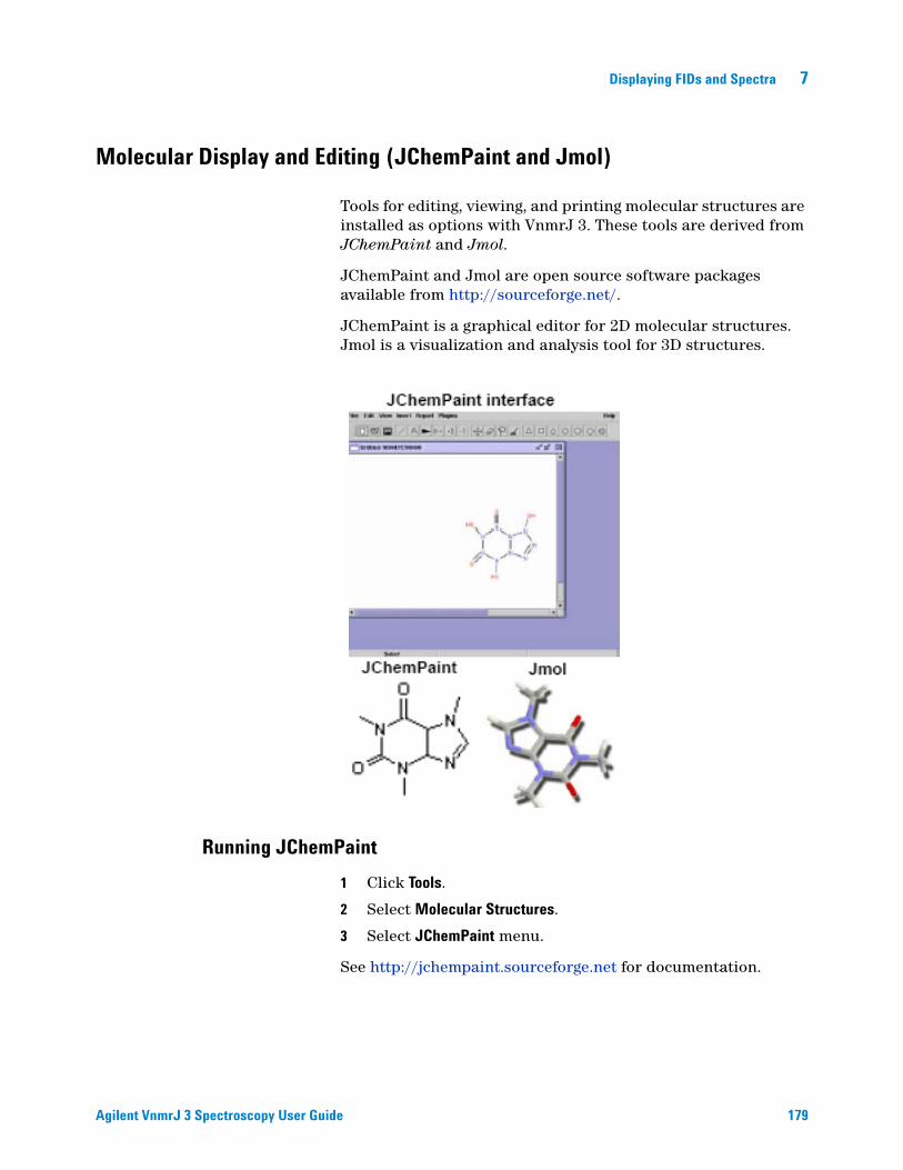
Displaying FIDs and Spectra 7
Molecular Display and Editing (JChemPaint and Jmol)
Agilent VnmrJ 3 Spectroscopy User Gui
Tools for editing, viewing, and printing molecular structures are installed as options with VnmrJ 3. These tools are derived from JChemPaint and Jmol.
JChemPaint and Jmol are open source software packages available from http://sourceforge.net/.
JChemPaint is a graphical editor for 2D molecular structures. Jmol is a visualization and analysis tool for 3D structures.
Running JChemPaint
1 Click Tools.
2 Select Molecular Structures.
3 Select JChemPaint menu.
See http://jchempaint.sourceforge.net for documentation.
de 179

7 Displaying FIDs and Spectra
File Formats
180
JChemPaint can edit, save, and export the file formats listed here.
1 Save files as MDL MOL (*.mol) in one of the mollib directories: /vnmr/mollib or ~username/vnmrsys/mollib.
2 Import an existing mol file into VnmrJ 3 by copying it into the mollib directory.
3 Click Tools on the main menu.
4 Select Open, browse to the file, and drag it to the VnmrJ 3 graphics screen.
Format Action
MDL MOL edit, save
SMILES edit, save
IUPAC Chemical Identifier edit
MDL SDF Molfile edit
Chemical Markup Language edit
Scalable Vector Graphics save
CDK source code fragment save
BMP save
JPEG save
PNG save
TIFF save
Gaussian Input export
Molecular structures
Molecular structures are displayed and manipulated in the VnmrJ 3 graphics window. View as many graphics as wanted. The graphics are displayed in the current experiment, and they are saved per experiment.
Agilent VnmrJ 3 Spectroscopy User Guide

Displaying FIDs and Spectra 7
Agilent VnmrJ 3 Spectroscopy User Gui
Use the following steps to display a molecular structure in the VnmrJ 3 graphics window:
1 Click Tools on the main menu.
2 Select Browser, browse to the mollib directory:
/vnmr/mollib or ~username/vnmrsys/mollib
3 Select the appropriate files and drag them to the VnmrJ 3 graphics window:
• Molecule file -- select a file from the mollib directory that ends in the mol extension.
• Graphic file -- open the icons directory and select a TIFF, GIF, JPEG, or PNG file.
After a molecular structure is displayed, use the mouse to move, resize, delete, or view the corresponding 3D version with Jmol.
To: Do:
Select Double-click the molecule.
Move Select the molecule and drag with the left mouse button.
Resize Select the molecule and drag with the middle mouse button.
Delete Select the molecule and drag to the trash can.
View a molecule with Jmol
Select the molecule and click the right mouse button. This only works with MOL files. See Jmol Interface in VnmrJ 3 Jmol Interface in VnmrJ 3.
de 181

7 Displaying FIDs and Spectra
Jmol interface in VnmrJ 3
182
VnmrJ 3 provides some Jmol tools to view a molecule.
Menu Description
Display H– Displays hydrogen atoms. Anti-Alias – Turns on anti-aliasing and smooths the graphics display. Measurements – Displays measurements.
Atom Type Displays the atoms with atomic symbols, atom types, atom numbers, or nothing.
View Views the molecule from front, tom, bottom, right, or left.
Mode Rotate – rotates the image.Zoom – zooms in/out.Translate – moves the image.Select – selects the atoms.Measure– measures distance, angle, or dihedral. See “Measuring a molecule” on page 183.
Save Image Saves the molecule image as BMP, JPEG, PPM, PNG, or PDF. The image is saved in the directory ~username/vnmrsys/mollib/icons with the name entered in the field. See “Saving a molecule image” on page 183.
Agilent VnmrJ 3 Spectroscopy User Guide

Displaying FIDs and Spectra 7
Agilent VnmrJ 3 Spectroscopy User Gui
Measuring a molecule
1 Select the measure mode: distance, angle, dihedral.
2 Click the appropriate atoms to create the measurement:
• distance – click two atoms.
• angle – click three atoms
• dihedral – click four atoms
3 Display the measurement by selecting the Measurement display option.
Saving a molecule image
1 Select the file format for the image: BMP, JPG, PPM, PNG, or PDF.
2 Enter a name for the image and add a file extension that corresponds to the file format chosen in step 1.
3 Press Enter.
The file is saved in the directory ~username/vnmrsys/mollib/icons/.
Jmol display options
• Change the foreground color of the molecule window: enter the following command on the VnmrJ 3 command line:
vnmrjcmd('mol','foreground','color')
where color is a color name or a hex value. The foreground color by default is set to the most visible color according to the background color.
• Change the font of the labels on 3D molecule graphics: use the Edit > Display Options window and change the font of Plain Text.
• Click to exit Jmol.
Full-Featured Jmol
Select Tools > Jmol to view a molecule with the full-featured Jmol software package,
See http://jmol.sourceforge.net/ for Jmol documentation.
Licenses for JChemPaint and Jmol
The licenses for JChemPaint and Jmol are included on the VnmrJ 3 CD in the licenses directory.
de 183

184
7 Displaying FIDs and Spectra
Agilent VnmrJ 3 Spectroscopy User Guide

Agilent VnmrJ 3 SpectroscopyUser Guide
8Printing, Plotting, and Data Output
Printing of the Graphics 186
Plotting 190
Plot Designer 195
Color Printing and Plotting 207
Sending a Plot via email 210
Pasting text into a Text Editor or Other Application 211
Advanced Printing Commands 212
Advanced Plotting Commands 214
This chapter describes how users can print and plot data.
Figure 32 A general printout with several objects identified
185Agilent Technologies

8 Printing, Plotting, and Data Output
Printing of the Graphics
186
After processing, the 1D or 2D spectrum is displayed in the graphics canvas so that the scale, expansion, and threshold can be adjusted.
To print the spectrum:
1 Click File from the menu.
2 Select Print Screen.
The pop-up in Figure 33 appears.
3 Select the name of the printer to print to it.
4 Select the print area, either Viewports or VnmrJ 3 Window. Viewport will capture the contents of the Viewport, while VnmrJ 3 Window will capture the entire VnmrJ 3 window.
5 Choose the number of copies to print.
6 Click the Print or the Preview button.
Figure 33 General tab of the Print Graphics pop-up
Agilent VnmrJ 3 Spectroscopy User Guide

Printing, Plotting, and Data Output 8
Printing a file
Agilent VnmrJ 3 Spectroscopy User Gui
Select the Print to file check box. Figure 34 shows the pop-up that appears when the Print to file check box is selected and the Print button is clicked.
• File Name: name of the file to be saved.
• Browse…: allows one to browse to a folder to set the location where the file will be saved.
• Format: drop-down menu that offers a choice of various outputs.
• Size: drop-down menu that offers choice for paper size.
• Orientation selection: radio-button to set Portrait or Landscape.
• Graphics color: radio-button to select Color or Monochrome output.
• Background and Foreground color selection: Pull-down menus for various color choices.
• Spectrum Line Width: spectrum line width in pixels.
• Graphics Line Width: graphics line width in pixels.
• Image Resolution: image resolution in dots per inch.
Figure 34 The Print to File pop-up
de 187

188
8 Printing, Plotting, and Data Output
• Screen resolution: the current screen resolution in dots per inch.
• Keep cursor lines: check box to include cursor lines as they appear in the graphics area.
• Reshape graphics to fit paper: check box to resize graphics to fit paper size.
• Save: saves output to File Name.
• Preview: starts Adobe Acrobat Reader and displays (without saving) the output.
• Cancel: closes Print to File pop-up (without saving).
The Page Setup and Appearance tabs (Figure 35 and Figure 36) allow for settings similar to the Print File Setup to be applied to the printed output. Additionally, entries are available for paper source, margins, and print quality (Draft, Normal, and High) while finer control of image resolution and preview is unavailable.
• Paper Source: drop-down menu choices for tray a printer will use.
• Margins: margins on the sides of the page in inches (in).
Figure 35 The Page Setup tab of the Print Graphics pop-up
Agilent VnmrJ 3 Spectroscopy User Guide

Printing, Plotting, and Data Output 8
Agilent VnmrJ 3 Spectroscopy User Gui
• Quality: a choice of Draft, Normal, and High.
Figure 36 The Appearance Setup tab of the Print Graphics pop-up
de 189

8 Printing, Plotting, and Data Output
Plotting
190
Plotting is based around the concept of a plot file. Setting up and submitting a plot can be done from the vertical and horizontal panels and from the command line. The Plot parameter page is accessed from the Process tab after the spectrum or FID is displayed. Items selected on the Plot parameter page (Figure 37 and Figure 38) are added to a temporary plot file, and the Plot Page button submits the plot file to the plotter.
Figure 37 The Plot parameter page for a 1D data set
To plot: Select: Click:
Pulse sequence Plot Pulse Sequence
FID Plot FID, Plot Page
FID and scale Plot FID, Plot FID Scale, Plot Page
Spectrum Plot Spectrum, Plot Page
Spectrum and scale Plot Spectrum, Plot Spectrum Scale, Plot Page
Spectrum, scale, and text
Plot Text, Plot Spectrum, Plot Spectrum Scale, Plot Page
Spectrum, scale, and parameters
Parameter Template option
Plot Spectrum, Plot Spectrum Scale, Plot Page
Spectrum, scale, and peak frequencies
Peak Frequencies option
Plot Spectrum, Plot Spectrum Scale, Plot Page
Spectrum, scale, and integrals
Plot Spectrum, Plot Spectrum Scale, Integrals Plot, Plot Page
Agilent VnmrJ 3 Spectroscopy User Guide

Printing, Plotting, and Data Output 8
Agilent VnmrJ 3 Spectroscopy User Gui
The Clear Plot button removes the plot file. The Plot Preview button starts Adobe Reader (Figure 39) and displays the output of the plot file. Some of the menu options in Adobe Reader are available for use. The Automatic Plot Page button executes the plot macro; then the resetplotter macro and the Auto Plot Preview button executes the macro pageview(‘auto’) to generate the output. The PlotView
Spectrum, scale, and integrals, integral values
Integrals option Plot Spectrum, Plot Spectrum Scale, Integrals Plot, Plot Page
Parameters only Parameter Template option
Plot Page
Text only Plot Text, Plot Page
Peak frequencies only Peak Frequencies option
Plot Page
Integrals only Integrals option Integrals Plot, Plot Page
Scaled integral values only
Integrals option Integrals Plot, Plot Page
Normalized integral values only
Integrals option Integrals Plot, Plot Page
Molecules only Plot Molecules, Plot Page
Logo only Plot Logo, Plot Page
Using default settings to the printer
Automatic Plot Page
Using default settings to Adobe Reader for preview
Auto Plot Preview
Figure 38 The Plot parameter page for a 2D data set
To plot: Select: Click:
de 191

192
8 Printing, Plotting, and Data Output
pop-up (Figure 40) appears during a preview, which allows the saving of the view to a pdf format file, sending the output to the default plotter, a file, and to one or more e-mail addresses.
The Plot parameter page for a 2D data set contains both- the show and plot buttons. Plot adds to a temporary plot file, show displays in the graphics area.
Figure 39 Preview of the plot file initiated from pressing the Plot Preview button
Figure 40 The PlotView pop-up
Agilent VnmrJ 3 Spectroscopy User Guide

Printing, Plotting, and Data Output 8
Agilent VnmrJ 3 Spectroscopy User Gui
The Basic parameter page (Figure 41) contains Plot and a Plot Preview buttons; both have the same function as the Automatic Plot Page and Auto Plot Preview buttons found on the Plot parameter page.
Figure 41 The Basic parameter page for a 1D data seThe 1D Vertical parameter page contains four buttons in the Basic Plotting group.
• Auto Plot Page does the same function as the Automatic Plot Page button in the Plot parameter page.
• Auto Plot Preview button does the same function as the Plot parameter page.
• Print Screen… button does the same function as File / Print Screen.
• More Plotting – Parameter Pages button opens the horizontal panel and displays the Plot parameter page.
de 193

194
8 Printing, Plotting, and Data Output
Figure 42 The 1D Vertical parameter page
Agilent VnmrJ 3 Spectroscopy User Guide

Printing, Plotting, and Data Output 8
Plot Designer
Agilent VnmrJ 3 Spectroscopy User Gui
Plot designer provides the following tools:
• Interactive plot composition fine-tuning of the layout on the screen prior to plotting.
• Label spectra with text in various fonts and draw lines, boxes, and arrows.
• Save customer plot layouts and templates for reuse.
• Export plots for further annotation and incorporation into reports and publications.
System requirements
Plot Designer is a Java-based application. The Java Runtime Environment (JRE) provides an environment in which Java applications run. Any required updates are available from the update area of the Sun Microsystems Web site at http://www.sun.com.
Using plot designer
Select a viewport and process the data set for plotting.Start the Plot Designer program as follows:
1 Click File.
2 Select Create a Plot Design.
The Plot Designer window opens. See Figure 43.
Figure 43 Plot Designer with current default template
de 195

196
8 Printing, Plotting, and Data Output
3 Load a template:
a Click File.
b Click Templates.
c Click Plot Template.
d Select from the following standard templates or any custom user-created template:
e Select Use this template as default to keep this as the template that loads each time Plot Designer is started. The name of the default template is shown on the message line above the Plot Templates window control buttons.
f Click Open.
4 Select Preview from the Plot Designer menu.
5 Select All.
The data from the active viewport is imported into the various regions of the template based upon the commands associated with each region.
deptB dicom.default chemParray chemP1d
basic2D oneD Whitewash ChemP2d
Figure 44 Default oneD template with imported data
Agilent VnmrJ 3 Spectroscopy User Guide
Printing, Plotting, and Data Output 8
Creating a customized template
Agilent VnmrJ 3 Spectroscopy User Gui
Create a template from scratch or base a customized template on one of the supplied templates.
To prepare to customize a template:
1 Start Plot Designer.
2 Click File.
3 Select Create a Plot Design.
4 Load a template or use the default template.
5 Do any or all of the following:
• Click a region to delete. See “Deleting a region” on page 197.
• Delete all the regions. See “Clearing all regions from the workspace permanently” on page 197.
• Add a new region. See “Adding a region” on page 198.
• Edit an existing region: double on a region, click Region on main menu, select Edit, and enter the plotting command for the content of the selected region. See “Editing plotting commands in a new or existing plot region” on page 198
• Add text and graphics elements: see “Adding and editing text and graphics elements” on page 199.
Deleting a region
1 Double-click a region.
2 Click Region-Delete.
Restoring a single deleted region
Click Region-Undelete.
Clearing all regions from the workspace permanently
Click Delete All: no undelete. Regions removed with Delete All cannot be restored with Undelete.
de 197

8 Printing, Plotting, and Data Output
Adding a region
198
1 Click Region on main menu.
2 Select New (mouse cursor changes to a cross hair).
3 Draw the new region on the screen.
Editing plotting commands in a new or existing plot region
1 Double-click a region to make it active. Active regions have red borders with control handles.
2 Enter new plotting commands or edit existing plotting commands in the region editor window. Any plotting currently support plotting command is allowed.
The Region Editor window control buttons as listed in Table 9 are found.
Figure 45 Editing a plot region commands
Table 9 Region editor buttons
Button Function
Restore Applies the original template to a region. Restores template to its original design if it was opened and changes were made to it, using this button.
Delete Removes text. This option is not similar to Copy. Deleted text is not stored in a buffer. Do not use Delete to cut and paste text.
Delete all Clears all text from the input area.
Copy Duplicates text.
Agilent VnmrJ 3 Spectroscopy User Guide

Printing, Plotting, and Data Output 8
Agilent VnmrJ 3 Spectroscopy User Gui
Paste Inserts copied text in the input area.
Close Exits the Region Editor.
Table 9 Region editor buttons (continued)
Button Function
Resizing and moving plot regions and objects
Move an object or region by double-clicking on it and dragging the mouse across the workspace. The arrow keys can be used to move objects.
Resize a region by double-clicking on it, grabbing a control handle (see Figure 45) on the border, and dragging it to the new size.
Adding and editing text and graphics elements
Change the size and color of objects in a region with the Item Preferences window, shown in Figure 46.
Click Region-Preferences to open this window or click the Item Preferences icon , described in “Plot designer tools” on page 202.
Figure 46 Item preferences window
de 199

8 Printing, Plotting, and Data Output
Changing line width
200
Change the width of a line by doing the following procedure:
1 Highlight the line or region by double-clicking on it.
2 Enter a new width in the Line Width field.
3 Click Apply to change the line.
4 Click anywhere in the workspace to deselect the line.
Changing fonts
Plot Designer has three font families: Sans Serif, Monospace, and Serif. Fonts can be Plain, Bold, or Italic. Change the family, style, and size of a font as follows:
1 Highlight the text or region.
2 Click the Item Preferences tool to open the Item Preferences window.
3 Choose a family, style, and enter a size in the Font field.
4 Click Apply to change the text.
Changing colors
Change the color of a line by doing the following:
1 Highlight the line or region.
2 Click the color button to open a pop-up menu showing a range of colors.
Move the tuning slider either left or right to change a color, or change a color by clicking on the left or right arrows in the Red, Green, and Blue fields. The values in the Color (RGB) field automatically change as the slider moves.
3 Click Apply when the required colors are selected.
4 Place the cursor anywhere in the workspace and click once to apply the color change.
Agilent VnmrJ 3 Spectroscopy User Guide

Printing, Plotting, and Data Output 8
Adding Text
Agilent VnmrJ 3 Spectroscopy User Gui
Do the following to add text into your design:
1 Click the text input tool to open the text input window.
2 Type text in the field at the top of the window.
3 Customize the text by clicking on the desired options and entering a font size in the indicated field.
4 Click Put and drag the cursor into the workspace, then click once to paste in the text.
Use the following procedure to copy and paste text that is already on the workspace and change the font styles:
1 Highlight the text.
2 Click the text input tool to open the Text Input window shown in Figure 46.
3 Select a Font family and Font style, and enter a Font size.
4 Click Put to paste the text in the workspace.
Figure 47 Text input window
Changing font color
Repeat the procedure given in“Changing colors” on page 200 to change font colors.
de 201
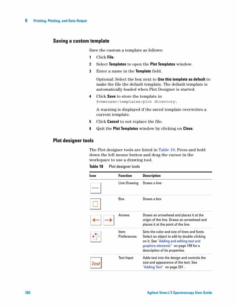
8 Printing, Plotting, and Data Output
Saving a custom template
202
Save the custom a template as follows:
1 Click File.
2 Select Templates to open the Plot Templates window.
3 Enter a name in the Template field.
Optional: Select the box next to Use this template as default to make the file the default template. The default template is automatically loaded when Plot Designer is started.
4 Click Save to store the template in $vnmruser/templates/plot directory.
A warning is displayed if the saved template overwrites a current template.
5 Click Cancel to not replace the file.
6 Quit the Plot Templates window by clicking on Close.
Plot designer tools
The Plot designer tools are listed in Table 10. Press and hold down the left mouse button and drag the cursor in the workspace to use a drawing tool.
Table 10 Plot designer tools
Icon Function Description
Line Drawing Draws a line
Box Draws a box
Arrows Draws an arrowhead and places it at the origin of the line. Draws an arrowhead and places it at the point of the line
Item Preferences
Sets the color and size of lines and fonts. Select an object to edit by double-clicking on it. See “Adding and editing text and graphics elements” on page 199 for a description of its properties.
Text Input Adds text into the design and controls the size and appearance of the text. See “Adding Text” on page 201 .
Agilent VnmrJ 3 Spectroscopy User Guide

Printing, Plotting, and Data Output 8
Agilent VnmrJ 3 Spectroscopy User Gui
Erasers The ALL eraser removes all objectsThe eraser tool removes selected objects. See also “Adding and editing text and graphics elements” on page 199, “Adding a region” on page 198, and “Deleting a region” on page 197.
Print Prints a file
Table 10 Plot designer tools (continued)
Icon Function Description
Changing an aspect or property of plot designer
1 Click Preferences from the main menu.
2 Select Set Up to open the Workspace Preferences panel.
3 Click the corresponding button to open a pull-down menu.
4 Select a color preference.
5 Click Apply to execute the changes.
6 Click Close to exit the window.
de 203

204
8 Printing, Plotting, and Data Output
Table 11 Workspace preference controls
Control Function
Background Changes the background color of the window
Border Color Changes the color of the border surrounding the workspace
Highlight Color Color of an object after double-clicking on an object to indicates that it is selected
Grid Color Changes the color of the grid
Plotter Selects a black and white or color plotter
Border Shows (on) and hides (off) region borders
Grid Shows (on) and hides (off) grid in the workspace
Snap The center of the border of an object snaps to the grid when an object is created or moved if snap is turned ON. Turn Snap OFF to disable this feature.
Snap Spacing Controls the amount of space on the grid to which an object snaps. Spacing is in inches, centimeters, or points.
Changing the shape of the plot designer window
Plot Designer can be viewed in two orientations- Landscape or Portrait (which is the default orientation). Change the shape of the Plot Designer window in the Orientation menu.
Changing the size of the plot designer window
Increase or decrease the size of the Plot Designer window by clicking on the sizes listed in the Magnify menu.
Saving a Plot File
Do the following procedure to save a plot:
Figure 48 Plot save window
Agilent VnmrJ 3 Spectroscopy User Guide

Printing, Plotting, and Data Output 8
Agilent VnmrJ 3 Spectroscopy User Gui
1 Click File in the Main Menu, then Save Data to open the Plot Save window shown in Figure 48.
2 Scroll down the list of directories and choose a directory or enter a path for the file in the Directory field.
3 Select a Data format for your file and enter a Data resolution. Table 12 lists the formats that are available.
Table 12 Output formats supported by plot designer
Format Description
AVS AVS X image file
BMP Microsoft Windows bitmap image file
EPS Adobe Encapsulated PostScript file
FAX Group 3 FAX
FITS Flexible Image Transport System
GIF Compuserve Graphics Interchange Format (version 89a)
GIF87 Compuserve Graphics Interchange Format (version 87a)
JPEG Compressed format from Joint Photographic Experts Group
MIFF Magick image file format
PCD Photo CD
PCX ZSoft IBM PC Paintbrush file
PDF Portable Document Format
PICT Apple Macintosh QuickDraw/PICT file
PGM Portable gray map
PNG Portable Network Graphics
PS Adobe PostScript file
PS2 Adobe Level II PostScript file
SGI Irix RGB image file
SUN Sun Rasterfile
TGA Truevision Targa image file
TIFF Tagged Image File Format
VIFF Khoros Visualization image file
XBM X11 bitmap file
XPM X11 pixmap file
XWD X Window System window dump image file
de 205

206
8 Printing, Plotting, and Data Output
4 Label your file by entering a name in the File field.
5 Click Close to exit the window.
Printing a plot
Click the print tool.
Exiting plot designer
Click File-Quit.
Any design in the window when Plot Designer is closed is automatically opened in the workspace the next time the program is started.
Agilent VnmrJ 3 Spectroscopy User Guide

Printing, Plotting, and Data Output 8
Color Printing and Plotting
Agilent VnmrJ 3 Spectroscopy User Gui
Printer and Plotter color output is defined using the Styles and Themes window, which provides access to the display colors and the VnmrJ 3 interface colors.
Setting colors
View the current settings or define new color settings as follows:
1 Click Edit.
2 Select Display options.
The Style and Themes window opens. See Figure 49.
Figure 49 Styles and themes for display and 2D colors
de 207

208
8 Printing, Plotting, and Data Output
3 Select the Display tab to set the colors for the spectra, axis, parameters, etc.
4 Click the Display and Output selection drop-down menu.
5 Select the output device: Display, Plot Postscript, Plot PCL, or Plot HPGL.
6 Select a color or keep the current color for each display or function shown.
7 Enter a name in the field next to the Save button to save the selection to a user defined file or continue with the next step to overwrite the current file.
8 Click Save to save the color selections to the specified file.
9 Click 2D colors.
10 Click Phase to set the colors for this 2D display mode.
11 Select the output device: Display, Plot Postscript, Plot PCL, or Plot HPGL.
12 Select a color or keep the current color for each contour level.
13 Click Absolute to set the color for this 2D display mode.
14 Select a color or keep the current color for each contour level.
15 Enter a name in the field next to the Save button to save the selection to a user-defined file or continue with the next step to overwrite the current file.
16 Click Save to save the color selections to the specified file.
Loading a color file
To retrieve a color file:
1 Select a theme file from the Theme drop-down menu.
2 Click Load.
Changing or renaming a color file
To change the colors in a file:
1 Select a theme file from the Theme drop-down menu.
2 Click Load.
3 Follow the procedure in “Setting colors” on page 207.
4 Click Save to save the file.
Agilent VnmrJ 3 Spectroscopy User Guide

Printing, Plotting, and Data Output 8
Agilent VnmrJ 3 Spectroscopy User Gui
To change the name of a color file:
1 Select a theme file from the Theme drop-down menu.
2 Click Load.
3 Enter a new name in the field next to the Save button.
4 Click Save to save the file.
5 Optional: To delete the file with the old name, see “Removing a color File” on page 209.
Removing a color File
To remove a color file from the list:
1 Select a theme file from the Theme drop-down menu.
2 Click Load.
3 Click Delete.
The deleted file is removed from the bottom list box.
4 Click OK, when prompted, to delete the file, or Cancel to keep the file.
Closing the color selection window
Click Close to exit the window.de 209

8 Printing, Plotting, and Data Output
Sending a Plot via email
210
After selecting the options to and clicking the Plot Preview button in the Plot parameter page.
1 Enter a Plot name in the PlotView pop-up.
2 Select File.
3 Select e-address.
4 Enter valid email addresses in the entry field of e-address.
5 Press the Plot / Save / Email button.
6 Press the Close button when done.
There are advanced macros that can be issued from the command line (eplot, epage, espec, fplot, fpage, efid, esampledir), which can be used to send the output to an email address. See the Command and Parameter Reference for details on the usage of the macros.
Agilent VnmrJ 3 Spectroscopy User Guide

Printing, Plotting, and Data Output 8
Pasting text into a Text Editor or Other Application
Agilent VnmrJ 3 Spectroscopy User Gui
Text output that appears in the Integration, Cursors/Line Lists/Text Output parameter pages can be pasted into a text editor or other application as shown in Figure 50, to be saved or used elsewhere.
1 Highlight the text to be pasted by clicking the left mouse button and dragging the mouse to the end of the desired text.
2 Release the mouse button at the end of the desired text. The selected text is highlighted indicating what has been selected.
3 Start the text editor or application and place the mouse cursor on the active document.
4 Click the middle mouse button to paste the highlighted text into the text editor.
Figure 50 Contents of the Display Line List text box copied into the Linux gedit text editor
de 211
8 Printing, Plotting, and Data Output
Advanced Printing Commands
212
Printing from within VnmrJ 3 is initiated with the printon command. Once the printon command is issued, all further output that normally appears in the text output window is redirected to a temporary file and no further output will appear in the text output window. When the printoff command is issued, the temporary file is sent to a printer, the file is purged from the system, and future text output is resumed to the text output window. This output includes the following:
• Parameter listings from dg, dgl, da, etc.
• Line listings from dll.
• Integral listings from dli.
• System configuration parameters generated by config ('display').
• Text files using the text command.
• Results of calculations from h2cal, adept, tl, t2, etc.
• Any other information that some program or macro may write to the text window.
This output is saved in a temporary file in the VnmrJ 3 subdirectory tmp. The VnmrJ 3 parameter printer determines the printer to which the output is directed. When the printoff command is issued, VnmrJ 3 executes a UNIX script called vnmrprint that sends the temporary file to the printer using standard UNIX printing utilities. This script is supplied with the name of the temporary file to be printed, the name of the printer (corresponding to a printcap entry), and the type of printer (corresponding to a devicetable entry).
NOTE The devicetable information is used to distinguish PostScript printers. The vnmrprint script allows users to customize.
The macro ptext(file) prints out the text file given as an argument. For example, the command ptext(’/vnmr/psglib/DEPT.c') prints the text file DEPT.c.
Print jobs for the currently active printer in VnmrJ 3 are held in a print queue. The showprintq macro displays the current print jobs in the print queue. The killprint macro will stop a print job and remove it from the print queue. Unless the user executing this macro is root (superuser), only that the user's print job is deleted from the print queue.
Agilent VnmrJ 3 Spectroscopy User Guide

Printing, Plotting, and Data Output 8
Agilent VnmrJ 3 Spectroscopy User Gui
Table 13 Printer-Associated commands and parameters
Commands
killprint Stop print job and remove from print queue
printoff<('clear'|file)> Stop sending text to printer and start print operation
printon Direct text output to printer
ptext (file) Print out a text file
showplotter Display currently defined plotters and printers
showprintq Display print jobs in print queue
vnmrprint* Print text files (UNIX)
* vnmrprint printfile <printcap> <printer_type <clear|file>>
Parameter
printer {string} Printer device
de 213

8 Printing, Plotting, and Data Output
Advanced Plotting Commands
Spectral plotting
214
The pl command plots the currently displayed region of the currently active spectrum, or spectrum plus integral (or the region which would be displayed if there were a spectral display on the screen). pl(’int’) plots the integral only. pl(’pen2’) plots the spectrum using pen number 2 of a multi-pen plotter.
The pscale command plots a scale under a spectrum. The syntax is:
pscale<(<axis><,vertical_start><,plot_start><,pen>)>
If the letter p, h, k, etc. is supplied as an optional argument for axis that is used instead of the current value of the parameter axis, the optional argument vertical_start defines the vertical position where the scale is drawn (the default is 5 mm below the current value of the parameter vp). The second optional argument plot_start is interpreted as a modified start of plot. The pen option defines the pen number to be used.
The ppf command plots peak frequencies in units specified by the axis parameter above the peaks, selecting only those peaks greater than th high. ppf(’noll’) plots peak frequencies using the last previous line listing while ppf(’pos’) plots only positive peaks. Other arguments for noise suppression (noise_mult) and label positioning work the same as the dpr command.
The pll command produces a columnar line list on a plotter, similar to what would appear on a printer. The output is automatically formatted into multiple columns, depending on the number of lines. The syntax is pll<(x,y,minimum_y)>. The arguments x and y are the x and y position of the upper left of the line list, and minimum_y is the minimum y at which to reset back to the top.
The plh command plots a proton spectrum based on parameters pltmod and intmod:
pltmod=’off’ sets no plotting.
pltmod=’fixed’ takes sp and wp as is.
pltmod=’full’ adjusts sp and wp to plot the full spectrum.
pltmod=’yariable’ adjusts sp and wp to plot only the region of interest.
intmod=’off’ gives no integral.
Agilent VnmrJ 3 Spectroscopy User Guide

Printing, Plotting, and Data Output 8
Agilent VnmrJ 3 Spectroscopy User Gui
intmod=’partial’ gives a series of integrals over each region.
intmod=’full’ gives a single integral over the entire spectrum.
Given a spectrum divided into regions by the region command or by the cursors in the ds program, the macro aexppl<(expansion_factor)> automatically plots each region at the horizontal scale requested (in Hz/ mm). The default scale is 2 Hz/ mm.
Several generic plotting macros, such as plot and plot1d, are available that call specialized plotting macros, depending on the user definition or other wise on the type of data in the experiment. For details, see VNMR Command and Parameter Reference.
Display limits
Because of the use of different plotters with different dimensions, the parameters sc, wc, sc2, and wc2 need to be set differently to position plots and displays in the same relative position on the page. The full, center, left, and right commands do nothing more than modify sc, wc, sc2, and wc2 to place the display and plot in the desired portion of the screen and page. The f command is used to set the sp and wp parameters to display a full spectrum. The zoom(width) macro adjusts the display limits to the width specified, in Hz, setting the limits to +/-width/2. Also available is the split macro, which repositions the left-hand cursor halfway between its original position and the position of the left cursor.
A scaling factor helpful for 1D plotting is the hzmm parameter, which contains the quotient of wp divided by wc.
The wysiwyg parameter is useful for scaling the image to a full window instead of the same size as the plot. Setting wysiwyg=’n’ sets a full display and wysiwyg=’y’ sets a plot display (the default).
Table 14 Plotting-Associated commands
Commands Descriptions
aexppl<(expansion_factor)> Automatic plot of spectral expansion
ap<(template)> Print out all parameters
bpa:$sc2_minimum Plot boxed parameters
hpa Plot parameters on special preprinted chart paper
killplot Stop plot job and remove from plot queue
page<(num_pages<,’clear’|file>)> Submit plot and change plotter page
de 215

8 Printing, Plotting, and Data Output
pap<(<template,>x,<,y><size>)> Plot out “all” parameters
pir Plot integral amplitudes below spectrum
pirn Plot normalized integral amplitudes below
pl* Plot spectra
plc<(pltmod)> Plot carbon spectrum
plh<(pltmod)> Plot proton spectrum
pll<(x,y,minimum_y)> Plot a line list
plp<(pltmod)> Plot phosphorus spectrum
plot Automatically plot spectra
plot1d Plotting macro for simple (non-arrayed) 1D spectra
ppf* Plot peak frequencies over spectrum
pscale* Plot scale below spectrum or FID
pltext* Plot text file
ppa<(x<,y>)> Plot parameter list in “English”
setpen<(maxpen,max_num_pen)> Set maximum number of HP pens
setplotdev<:plotter_type> Return characteristics of a named plotter
showplotq Display plot jobs in plot queue
showplotter Display currently defined plotters and printers
vnmrplot<file> Plot files (UN IX)
*pl<(<start,finish,step><,'int'><,'all'><,options>)>
*pltext<(<file><,x<,y<,width>>>)> <:$x_rext,$y_rext,$y increment>
*ppf<(<'noll'><,'pos'><,noise_mult><,'leader'><,length>)>
*pscale<(<'fid'><,axis><,yertical_start><,plot_start><,pen>)>
Plotting-Associated parameters
Parameters Descriptions
ap { string} “All” parameters display control
maxpen { 1 to number of pens} Maximum number of pens to use
plotter { string} Plotter device
wcmax { number, in mm} Maximum width of chart
Table 14 Plotting-Associated commands (continued)
Commands Descriptions
216 Agilent VnmrJ 3 Spectroscopy User Guide

Printing, Plotting, and Data Output 8
wc2max { number, in mm} Maximum width of chart in second direction
x0 { number, in mm} X -zero position of HP plotter or Postscript device
y0 { number, in mm} Y -zero position of HP plotter or Postscript device
hzmm { number} Scaling factor for plots
pltmod* Plotter display mode
sp { number, in Hz} Start of plot
wp { number, in Hz} Width of plot
* pltmod { ’ off’ ,’ fixed’ ,’ full’ ,’ standard’ ,’ user’ ,’ variable’ }
Plotting-Associated parameters (continued)
Parameters Descriptions
Agilent VnmrJ 3 Spectroscopy User Gui
de 217

218
8 Printing, Plotting, and Data Output
Agilent VnmrJ 3 Spectroscopy User Guide
Agilent VnmrJ 3 SpectroscopyUser Guide
9Advanced 1D NMR
Working with Experiments 220
Multi-FID (Arrayed) Spectra 222
Processing 226
T1 and T2 Analysis 229
Kinetics 232
Filter Diagonalization Method (FDM) 233
This chapter describes how to work with 1D NMR liquids experiments.
219Agilent Technologies

9 Advanced 1D NMR
Working with Experiments
220
In VnmrJ 3, NMR experiments are contained in Workspaces (also called experiments). Use the Locator to navigate to different workspaces.
1 Open up the Locator from within the Tools menu.
2 View the experiments in the Locator by clicking on the Locator Statements icon ( ) and selecting Sort Workspaces.
3 Open (connect to or join) an experiment by dragging it to the graphics window.
4 Create a new experiment (in sequential numerical order) by clicking on File > New Workspace.
5 Delete an experiment by dragging the experiment from the Locator to the trash can icon.
Enter explib. to view the experiments on a system in the Process / Text Output page. The output will show the library of the currently available experiment files (exp1, exp2,..., exp9999).
Although multiple experiments can be created, only one experiment at a time is allowed to be currently active in the foreground for manipulation. Simultaneously, background processing or acquisition can occur in other experiments.
To use the menu system to copy selected bits of information between Experiments:
1 Click Edit.
2 Select one of the following options:
• Move Parameters
• Move FID
• Move Text
• Move Display parameters
• Move Integral resets
3 Fill in the information requested in the pop-up window.
4 Join the new experiment if desired.
Agilent VnmrJ 3 Spectroscopy User Guide

Advanced 1D NMR 9
Agilent VnmrJ 3 Spectroscopy User Gui
These same functions can be accomplished on the command line by using the mp, mf, and md commands to move (copy) files between Experiments.
• mp(<n,>m) moves parameters from Experiment n to Experiment m, for example, mp(4,5). If n is omitted, parameters are moved from the currently active Experiment to Experiment m.
• mf(<n,>m) moves the last acquired FID and the associated parameters.
• md(<n,>m) moves only those “saved display” parameters associated with the commands s1 through s9.
de 221

9 Advanced 1D NMR
Multi-FID (Arrayed) Spectra
222
Many NMR experiments acquire a series of FIDs, related to each other through the variation of one or more parameters. For example, suppose it is necessary to run a series of spectra at four different temperatures: 30 °C, 50 °C, 70 °C, and 90 °C. Instead of acquiring four separate sets of data, it is possible to create an array in which the temp parameter is given four successively different values. These four subexperiments are now all treated as a single experiment. Entering go begins successive acquisition of all four experiments. One advantage of acquiring data like this – as an "array" – is that they can all be transformed, displayed, phased, referenced, plotted, and saved with single commands. Using arrays to acquire data has always been a very powerful feature of the Agilent software.
Arrayed parameters
Use the Array Parameter window (called from the Acquisition/ Parameter Arrays menu; see “Parameter Arrays” on page 120) to create an arrayed experiment. Alternatively, you can use the command line to create arrays by using either the array macro, or by entering the parameter and its desired arrayed values (separated by commas; that is, temp=30,50,70,90 or pw=5,10,15,20,25). Alphanumeric parameters can also be arrayed (that is, use dm='n','y' to perform two experiments in which the decoupler is off in the first experiment and on in the second experiment).
Not all parameters can be arrayed. Non-arrayable acquisition parameters include display parameters, most processing parameters, and any parameter that changes the number of data points to be acquired, such as np, sw, dp, and at.
To display the values of the currently arrayed parameter, either open the Array Parameter window or type da. The typed da command displays all values of arrayed parameters if entered without an argument. If one or more parameters are listed as an argument, da displays only the specified parameters.
Agilent VnmrJ 3 Spectroscopy User Guide

Advanced 1D NMR 9
Multiple arrays
Agilent VnmrJ 3 Spectroscopy User Gui
Two or more parameters can be arrayed in an experiment. For example, an experiment to perform a series of decoupling experiments using an array of decoupler power levels and an array of decoupler frequencies might be set up with dpwr=17,20,23 and dof=295,345,507,1245. In this example, twelve experiments are performed (for example, three different values of decoupler power dpwr are used for each of the four different values of the decoupler offset dof).
Setting array order and precedence
Whenever an array of one or more parameters is set up, the parameter array becomes important. This parameter tells the system the name of the parameter or parameters that are arrayed and the order and precedence in which the arraying is to take place. The Array Parameters window, see “Parameter Arrays” on page 120, may be used for setting all of the parameters associated with setting up the array.
The string parameter array can have one of several forms:
array= '' means no parameter is arrayed (this value is two single quotation marks with no space between, not a double quotation mark).
array='x' means parameter x is arrayed.
array='y,x' means parameters x and y are arrayed, with x taking precedence. The order of the experiments is x1y1, x2y1, ...xny1, x1y2, x2y2,...xmy2...xmyn, with a total of m×n experiments being performed. The order of precedence behaves the way an odometer would; right to left.
array='x,y' means parameters x and y are arrayed, with y taking precedence. The order of the experiments is x1y1, x1y2,...x1yn, x2y1, x2y2,...x2yn,...xmyn, with a total of m×n experiments being performed.
array='(x,y)' means parameters x and y are jointly arrayed (“diagonallized”). The number of elements of the parameters x and y must be identical, and the order of experiments is x1y1, x2y2, ...xnyn, with n experiments being performed.
Entering one or more arrayed parameters automatically sets up an array. It is necessary to enter the array directly only if the order or precedence needs to be changed.
All of these changes can also be accomplished within the Array Parameter window.
de 223

9 Advanced 1D NMR
Interactively arraying parameters
224
Separate from the array parameter is the array macro. Entering the array macro without an argument starts it in the interactive mode and it prompts for the following information in this order:
• The name of the parameter to be arrayed.
• The number of values of the parameter.
• The starting value.
• The step size (the difference between values in the array).
An arrayed parameter is set up using the information provided. The restrictions with this macro are that only numeric parameters can be arrayed and all values of the array must satisfy the limits of the parameter.
Entering an array with a parameter name as an argument, (for example, array('pw')) still starts an interactive mode, but the program only asks for the remaining three items of information. Alternatively, an array bypasses the interactive mode completely if it is started with all four arguments (in the proper order: parameter name, number of steps, starting value, and step size). For example, entering array('tof',5,1000,-50) sets the tof parameter to have 5 elements with the values in the order 1000, 950, 900, 850, 800.
Resetting an array
Once an array is created, it is possible to change the value of a single element of the array by typing, for example, pw[2]=11.3, where the 2 enclosed in brackets indicates which element of the array to modify (array elements are counted starting at 1). This can also be done within the Array Parameter window.
Set a single value for the parameter (for example, pw=10) to reset an arrayed parameter to a single value. The array parameter is automatically modified to reflect this change.
Array limitations
Regular multiple arrays can include up to 20 parameters, each of which can be a simple parameter or a diagonal array (a set of parameters), which can include up to 10 parameters. The total number of elements of all arrays is essentially unlimited (232–1).
Agilent VnmrJ 3 Spectroscopy User Guide

Advanced 1D NMR 9
Acquiring data
Agilent VnmrJ 3 Spectroscopy User Gui
Once any parameter is arrayed, acquisition generates not just one, but an entire array of spectra. These spectra can then be examined either individually or as a group, as described below.
Autogain cannot be used in an arrayed experiment. Either use gain='y', which sets the gain to the previously determined value, or set the gain equal to a fixed value. The gain parameter itself cannot be arrayed.
Arrayed acquisitions can be interleaved, in which, a part of each experiment is done in turn rather than starting and finishing each experiment sequentially. The interleave function is controlled by the parameters il and bs.
• il='y'
Experiments are interleaved: bs transients are performed for each member of the array, followed by bs more transients for each member of the array, which continues until nt transients are collected for each member of the array. Thus, il is relevant only if bs (block size) is less than nt (number of transients).
• il='n'
All nt transients are acquired for the first experiment in the array, then all nt transients for the second experiment, continuing until nt transients have been acquired for each member of the array. The bs parameter is still active, but it is not involved in interleaving when il='n'.
de 225
9 Advanced 1D NMR
Processing
226
The Transform, Transform all, and Process buttons reprocess all elements of the array. The typed commands ft or wft can also be used to transform all of the spectra. Both commands take the same arguments and options:
• 'acq' does not transform elements that have already been transformed.
• 'nods' prevents an automatic spectral display (same as ds command).
• 'zero' zeroes the imaginary channel of the FID before Fourier transform.
Phasing can be done on any spectrum. Only one set of phase correction parameters exists, so all spectra have the same phase at any one time (although the phase can of course be changed when examining different spectra).
Display and plotting
The Vertical Panel “Arrayed Spectrum” can be used for
displaying arrayed data. The command ds(index) or the
and icons, interactively display the requested spectrum
from the array. The index argument can have one, two, or three numbers, each separated by commas, depending on the size of the spectral array.
Note that spectra are always scaled according to the number of completed transients ct; if nt is arrayed (nt=1,2,4,8), each spectrum is scaled by its own ct.
Other spectra display commands are not interactive like the dc command: dss, dssn, dssa, dssan, dssh, dsshn, and dssl. They display stacked spectra in which each spectrum is offset with respect to the previous spectrum. The order of stacking can be left to right, right to left, top to bottom, or bottom to top, depending on whether the horizontal offset (ho) and vertical offset (vo) parameters are positive or negative. Some of these commands set ho and vo automatically.
Agilent VnmrJ 3 Spectroscopy User Guide

Advanced 1D NMR 9
Agilent VnmrJ 3 Spectroscopy User Gui
The spectra display commands function as follows:
• dss displays stacked spectra using the current values of ho and vo to set the order of stacking.
• dssn displays stacked spectra the same as dss, but the graphics window is not erased before starting the display. This allows composite displays of many spectra to be created.
• dssa displays stacked spectra automatically (that is, vo and ho are automatically adjusted to fill the screen in a lower left to upper right presentation).
• dssan displays stacked spectra automatically the same as dssa, but the graphics window is not erased before starting the display.
• dssh displays stacked spectra horizontally (that is, vo is set to zero, and ho is adjusted to fill the screen from left to right).
• dsshn displays spectra horizontally the same as dssh, but the graphics window is not erased before starting the display.
• dssl displays a label for each element in a set of stacked spectra. The label is an integer value starting with 1 and extending up to the number of spectra in the display. (Note that it always starts numbering with 1, regardless of which spectra are displayed.)
The command pl plots stacked spectra with the same format as displayed by dss.
The argument syntax <(start,finish<,step>)><,options>)> is used by the dss command, the variants of dss, and by the pl command. The arguments are the following:
• start is the index number of a particular trace to be viewed when displaying arrayed 1D spectra or 2D spectra. It is also the index of the first spectrum when displaying multiple spectra.
• finish is the index of the last spectra when displaying multiple spectra. Because the parameter arraydim is automatically set to the total number of spectra, if finish is set to arraydim, all remaining spectra in the array will be shown.
• step is the increment for the spectral index when displaying multiple spectra. The default step is 1.
Options can be any of the following:
• 'all' is a keyword to display all of the spectra.
de 227

228
9 Advanced 1D NMR
• 'int' is a keyword to display only the integral, independently of the value of the parameter intmod.
• 'top' or 'side' are keywords that cause the spectrum to be displayed either above or at the left edge, respectively, of a contour plot. This assumes that the parameters sc, wc, sc2, and wc2 are those used to position the contour plot. This option does not apply to dssa, dssan, dssh, or dsshn.
• 'dodc' is a keyword for all spectra to be drift corrected independently.
• 'red', 'green', 'blue', 'cyan', 'magenta', 'yellow', 'black', and 'white' are keywords that select a color. This option does not apply to dssa, dssan, dssh, dsshn, or pl.
• 'pen1', 'pen2', 'pen3', etc. specify a pen number on a plotter. This option does not apply to dss or any of its variants.
Pulse width calibration step-by-step (using an array)
Note, for illustration, how the following steps perform a pulse-width calibration using arrays:
1 Set up parameters and obtain a normal spectrum of any sample. For best results, one or more intense signals should appear near the center of the spectrum.
2 Enter 5 for the value of pw (for example, pw=5) or use some other small value.
3 Enter 1 for the value of nt (for example, nt=1).
4 Obtain a spectrum and phase it properly. Set d1 to 5* T1 (or set it to a long value like d1=10 if you do not know the T1).
5 Make an array of pw from 5 to 30 in steps of 5 or use some other set of suitable values for the pw array.
6 Select Absolute Intensity and acquire. For example, enter pw=5,10,15,20,25,30 ai go. (Absolute instensity mode is also set by Process / Display / Amplitude Scaling / Absolute.
7 Transform and display the stacked data after the experiment finishes acquisition (for example, wft dssh).
8 Find the experiment where the signal goes through its 360° (or 180°)null. Enter da to remind yourself of the values of the pw array.
9 Enter pw equal to one-quarter of pw360 (or, less desirably, to one-half of pw180) to reset the array.
Agilent VnmrJ 3 Spectroscopy User Guide

Advanced 1D NMR 9
T1 and T2 Analysis
Agilent VnmrJ 3 Spectroscopy User Gui
A common form of arrayed experiment is the "inversion-recovery T1" experiment. In this experiment the nuclei are allowed to relax to equilibrium (d1) then inverted with a 180° pulse (p1), given a variable time to return to equilibrium (d2), and finally given a monitoring 90° pulse (pw) to measure their peak height as a function of d2. Under most circumstances, the behavior of the peak heights as a function of d2 will be exponential and this exponential time constant is the T1.
Setting up the experiment
The standard two-pulse sequence is used to perform the T1 experiment. The experiment can be set up by using any one of the following three methods.
1 Entering appropriate values for p1, pw, d1, and an array of values for d2.
2 Using the dot1 macro.
dot1 sets up all parameters to perform a T1 experiment, including d1, pw, p1, nt, and an array of d2 values, based on information entered. The three arguments that can be input are the minimum expected T1, the maximum expected T1, and the total time in hours the experiment should take. If no arguments are provided, dot1 prompts the user for the information.
3 Click the T1_measure protocol button, or use the menu as follows:
a Click Experiment.
b Select H1 Relax. Measurements.
c Select T1 Measurements.
d Fill in the information on the Standard panel of the Start tab.
e Adjust parameters on the Acquire / Defaults page.
The parameter pw90 must contain a correctly calibrated 90-degree pulse width because dot1 uses this information.
de 229

9 Advanced 1D NMR
Processing the data
230
Once the data is acquired and transformed, use one of the following two methods to set up the data for analysis.
1 Go to the Process / T1 Analysis panel, and follow the directions listed there.
2 Display the last spectrum of the T1 arrayed dataset.
3 Phase this spectrum properly.
4 Select a threshold and adjust the threshold line position.
5 Enter dpf, or dll, or click the appropriate button to display a line list and locate lines for the system.
6 Enter fp to "find peaks" (measure the peak height of each peak in an array of spectra). If optional line indexes are supplied to fp as arguments (for example, fp(1,3)), only the peak heights of the corresponding lines are measured.
7 Type t1 to run the T1 analysis.
The npoint parameter (if defined and set “on”) determines the range of data points over which the fp command searches for a maximum for each peak.
Analyzing the data
T1 and T2 analysis is performed by the t1 and t2 macros, respectively. t1 and t2 measure relaxation times for all lines in the line listing and display an extended listing of observed and predicted peak intensities. t1s and t2s perform the same calculation as t1 and t2, but produce a shorter output, showing only a summary of the measured relaxation times.
The Process / T1 Analysis / Display All Fits button, or the command expl, displays the exponential/polynomial curves resulting from T1 and T2, or kinetic analysis. Optional input of line numbers as arguments allows you to display only selected lines. Similarly, the command pexpl will plot the same curves.
The macro autoscale returns the command expl to autoscaling, in which scale limits (set by scalelimits) are determined that will display all the data in the expl input file. The macro scalelimits causes the command expl to use typed-in scale limits. If no arguments are given, scalelimits asks for the desired limits. The limits are retained as long as an expl display is retained.
Agilent VnmrJ 3 Spectroscopy User Guide

Advanced 1D NMR 9
Agilent VnmrJ 3 Spectroscopy User Gui
Enter dels(index1<, index2>...) to delete spectral data from the t1 or t2 analysis (or from t1s or t2s). This command deletes data, for the spectra selected by the indexes, from the output file fp.out that is used by the t1 or t2 analysis. The deleted data can be restored by rerunning fp.
T1 data workup: step-by-step
The following procedures accomplish a manual T1 analysis:
1 Enter rt('/vnmr/fidlib/T1_measure_01.fid').
2 Enter wft dssh full ds(arraydim) aph.
3 Use the left mouse button to set the threshold.
4 Enter dll fp t1 center expl.
de 231

9 Advanced 1D NMR
Kinetics
232
The arraying capability of the VnmrJ 3 software provides for the acquisition of data for the study of kinetics.
Setting up the experiment
Typically, the best procedure is to array the preacquisition delay parameter pad. For example, if pad=0,3600,3600,3600,3600, the system acquires the first spectrum immediately (pad[1]=0), waits 3600 seconds (pad[2]=3600), acquires the second spectrum, waits another 3600 seconds, etc. Because 3600 seconds is 1 hour, this inserts a wait of one hour between acquisitions. After all the spectra have been obtained, they are processed much like T1 or T2 data.
Processing the data
If the signal decreases exponentially with time, the output is matched to the equation:
I=A1*EXP(-T/TAU)+A3
The analysis is done by the macro kind or by macro kinds if a short output table is desired.
If the signal increases exponentially with time, the output is matched to the equation:
I=-A1*EXP(-T/TAU)+A3-A1
with analysis done by the macro kini, or by the macro kinis for a short output table.
Kinetics step-by-step
The following steps are typical in processing a kinetics experiment using the command line:
1 Enter wft dssh full ds aph.
2 Click the Threshold icon in the Graphics Control menu. Use the left mouse button to set the threshold.
3 Enter dll fp.
4 Enter kind, kini, kinds, or kinis, as appropriate.
5 If desired, adjust sc, wc, sc2, and wc2 by entering center or full.
6 Enter expl.
Agilent VnmrJ 3 Spectroscopy User Guide

Advanced 1D NMR 9
Filter Diagonalization Method (FDM)
Agilent VnmrJ 3 Spectroscopy User Gui
Filter Diagonalization Method is an optional package that must be purchased and installed. Installation requires a password.
Filter Diagonalization Method (FDM) is a non-Fourier data-processing method that extracts spectral parameters (peak positions, line widths, amplitudes, and phases) of Lorentzian lines directly from the time-domain signal by fitting FID data to a sum of damped complex sinusoids. The spectral parameters (saved in curexp/datdir/fdm1.parm) are also called “line list” and are used to construct an “ersatz” spectrum of the NMR data.
FDM is slower than Fast Fourier Transform, but it offers better resolution in the case of truncated signals and it has the option of processing only a selected spectrum region. FDM has the potential to work well with corrupted data, and the potential to produce a line list with each line representing a true NMR peak.
FDM reads input parameters from a file created by the fdm1 macro, using default (optimal) values. Change any of the parameters from the command line as needed. Table 15 lists fdm1 parameters. If the spectrum is not referenced with rl, the reference rfl is also read from curpar in the local parameter set. The section Changing Local FDM Variables Changing Local FDM Variables describes how to override the default setting.
In most cases, the only parameters that need to be set are the number of data points to be used and the spectrum window to be processed. The default setting uses half of the FID data or 3000 data points, whichever is smaller.
Table 15 fdm1 parameters
Parameter Description
Cheat No cheat if cheat=1, lines are narrower if cheat<1
Cheatmore No cheatmore if cheatmore=0
Error Error threshold for throwing away poles
Fdm 1 for fdm, • 1 for dft
Gamm* Smoothing width (line broadening)
Gcut Maximum width for a pole
Idat −4 for ASCII complex FID file, −5 for FID file
Kcoef kcoef>0; use “complicated” dk(k). • 1 always preferred
Nb* Number of basis function in a single window
Nbc* Number of coarse basis vectors
de 233

234
9 Advanced 1D NMR
Nsig* Number of points to use, 3000 is ok
Nskip* Number of points to skip
Rho rho=1 is optimal
ssw A test parameter
t0 Delay of the first point
theta Overall phase of FID (rp in radians)
wmin Minimum spectrum frequency in hertz
wmax Maximum spectrum frequency in hertz
Table 15 fdm1 parameters (continued)
Parameter Description
Using FDM
The following steps describe how to do normal activities such as phasing, zooming in, zooming out, and processing a spectrum window with the fdm1 macro.
1 Display the FID data and use the right mouse button to select the data points to be used by FDM.
2 Process the data with ft (it uses all FID points), then display and reference the spectrum.
3 Place the cursor on a region of interest, zoom in on it, then type fdm1 or Process....1D FDM from the main menu. Selecting and not zooming in on a region causes the whole spectrum in display to be processed.
4 A new menu appears with Start and Abort buttons. The calculation might take a few seconds to a few minutes depending on the number of data points used and the size of spectrum window to be processed. To abort the process, click Abort. The process is finished when the message, “FDM Execution Stopped Successfully” is displayed. If the process is finished, display the spectrum.
Reprocessing a spectrum
The Start button is displayed in the Process...1D FDM... drop-down menu. Use this button to reprocess a spectrum.
Agilent VnmrJ 3 Spectroscopy User Guide

Advanced 1D NMR 9
Changing parameters
Agilent VnmrJ 3 Spectroscopy User Gui
Relevant fdm1 global parameters are displayed on the 1D FDM... popup window with current values. These parameters can be changed. The value of a global parameter is saved to curpar, and it remains the same until changed from the parameter panel or a new assignment using the command line is made. The parameters can also be changed from the fdm1 command line as described in the section Changing Local FDM Variables Changing Local FDM Variables .
FDM global parameters
The following FDM parameters are global.
• Nsig is the number of FID points to use. Initialize it with the right mouse button position (crf + deltaf) *sw. If Nsig=0, half of the FID data points or 3000, whichever is smaller, is used. Nsig can be changed from the command line Nsig=nnnn, the right mouse button (when the FID is displayed), or the command line fdm1('Nsig',nnnn). In general, the more peaks, the more data points it takes to fit the spectrum. Check the reliability of the FDM method by changing Nsig a few times, and reprocess the data to see if the result is the same.
• Nskip is the number of data points to skip at the beginning of a FID. By default, zero points are skipped. In some cases, baseline can be improved by skipping the first one or two points.
• Nb is the number of basis functions (poles) used to fit each of the windows in an FDM calculation. The default is 10. FDM breaks down the specified window into smaller windows. In general, bigger Nb gives better results, especially better baseline. Sensible values for Nb are between 10 and 50.
• Nbc is the number of additional poles (coarse basis functions) to be used. The default is zero, but setting Nbc to an integer larger than zero (typically 4-10) might improve the baseline.
• Gamm is the smoothing width (line broadening). The default is 0.2*sw/Nsig, which is about a tenth of the FT resolution. Typical values are 0.1 to 1.0.
Using bigger Nsig, Nb, Nbc, or a spectral window significantly slows down the calculation.
de 235

9 Advanced 1D NMR
Changing Local FDM Variables
236
FMD parameters that are not commonly used are set as fdm1 local variables. These parameters are listed with global parameters in Table 15 on page 233. Local variables can be changed only from the command line. Parameter values are lost after the completion of the macro. To use a value again, it must be reentered. Otherwise, fdm1 sets the value to the default. To change more than one local variable, enter the variables from the same command line.
Any of the FDM parameters in the fdm1 command and both global and local variables can be changed. Values entered from the fdm1 command override the default, the change from the 1D FDM panel, and the value selected with the cursor. Enter command line arguments by giving the parameter name in single quotation marks and a value separated by a comma, for example:
fdm1('cheat',0.8) fdm1('Nsig',3000) fdm1('Nsig',3050) fdm1('Nb',20) fdm1('Nbc',10,'Nb',20) fdm1('Nsig',3000,'Nb',20,'Gamm',0.5) fdm1('wmin',-1600,'wmax',1600) fdm1('wmin',-1600,'wmax',0)
cheat is a factor multiplied to the line width. There is no cheat when cheat=1; lines are narrower when cheat<1.
wmin is the minimum spectrum frequency in Hz. The default is sp+rfl-sw/2. wmin is the upper field.
wmax is the maximum spectrum frequency in Hz. The default is wmin+wp. wmax is the lower field.
The center of the full spectrum is zero.
Seeing parameter values
Parameters are set to their default values. Normally, it is not necessary to change these parameters. Values of local fdm1 parameters cannot be queried with echo. To see the values of all parameters used, look in the fdm1.inparm file created by the fdm1 macro in the datdir directory of the current experiment.
Agilent VnmrJ 3 Spectroscopy User Guide

Advanced 1D NMR 9
FDM References
Agilent VnmrJ 3 Spectroscopy User Gui
J. Chen and V. A. Mandelshtam, J. Chem. Phys. (2000) 112: 4429-4437.
V. A. Mandelshtam, J. Magn. Reson. (2000) 144: 343-356.
H. Hu, A. A. De Angelis, V. A. Mandelshtam and A.J. Shaka, J. Magn. Reson. (2000) 144: 357-366.
de 237

238
9 Advanced 1D NMR
Agilent VnmrJ 3 Spectroscopy User Guide

Agilent VnmrJ 3 SpectroscopyUser Guide
10Multidimensional NMR
Hadamard Spectroscopy 240
Real-Time 2D 251
2D Experiment Set Up 254
Data Acquisition: Arrayed 2D 255
Weighting 257
Baseline and Drift Correction 260
Processing Phase-Sensitive 2D and 3D Data 264
2D and 3D Linear Prediction 270
Phasing the 2D Spectrum (Both F1 and F2) 271
Display and Plotting 273
Interactive 2D Color Map Display 277
Interactive 2D Peak Picking 282
3D NMR 287
4D NMR Acquisition 293
2D NMR data are similar to arrayed 1D data in many respects. A series of FIDs are acquired in 2D experiments as a function of time (using one of the time variables in the pulse sequence) and transformed into a series of spectra. 2D experiments do not explicitly specify the values of the time array. Instead, the timing is specified by two parameters, sw1 and ni, that respectively describe the “2D” spectral width (to be discussed shortly) and the "number of increments" (which determines the number of elements in the array, and the number of different experiments).
239Agilent Technologies

10 Multidimensional NMR
Hadamard Spectroscopy
240
Hadamard spectroscopy is a technique for acquiring multidimensional data sets using a small number of transients and reconstructing the nD spectrum using a Hadamard transform based on selective excitation of a predetermined set of frequencies using Hadamard encoding. A waveform generator is required due to the complexity of the shaped pulses. On the 400MR and VnmrS consoles, a waveform generator is included on the RF broad of each channel.
Acquiring the data
A list of selectively excited frequencies is created from a 1D spectrum or other means. A series of shaped pulses is created from the frequency list using a Hadamard matrix to selectively excite or invert the signals of interest. The matrix size is greater than the number of frequencies in the list. A typical Hadamard matrix is shown in Figure 51.
The first shaped pulse selectively excites all of the frequencies in the 8 x 8 matrix above. A second shaped pulse selectively excites the first four frequencies and inverts the second four frequencies. Frequencies 1, 2, 5, and 6 are selectively excited, and frequencies 3, 4, 7, and 8 are inverted by the third shaped pulse. The process is repeated until each row of the Hadamard matrix has been acquired.
Figure 51 Hadamard Matrix
Processing the data
Hadamard processing in the indirect dimension is done by summing, adding, or subtracting the acquired data increments in combinations according to the Hadamard matrix elements. Each sum gives a trace corresponding to a frequency in the list and is placed at the appropriate frequency in the indirect dimension. Areas between the frequencies in the list are
Agilent VnmrJ 3 Spectroscopy User Guide
Multidimensional NMR 10
Agilent VnmrJ 3 Spectroscopy User Gui
zero-filled. The data sets acquired in the direct dimension are Fourier transformed to produce a 2D spectrum.
The trace for the first frequency in the list is usually found in the second row of the Hadamard matrix. The second row in an 8 x 8 Hadamard matrix is created by adding the first four acquired elements and subtracting the second four acquired elements. The process is repeated until all traces for the selected frequencies are complete. A Hadamard matrix is created that is greater in size than the number of frequencies and contains more Hadamard sums than are needed.
2D and higher dimensional experiments using the Hadamard method are run and processed in a significantly shorter time than the same experiment acquired using hypercomplex or TPPI methods. Current software supports only 2D versions of Hadamard spectroscopy.
Implementing the method
A list of frequencies used for 2D Hadamard spectroscopy is contained in the parameter htfrq1. The Hadamard matrix size is set to a value that is both greater than the number of frequencies contained in the parameter htfrq1 and a power of two multiplied by 1, 12, 20, or 28. All shaped pulses are created in the pulse sequence using Pbox.
Hadamard data is processed using ft2d (or one of its variations) with proc1='ht'. The zero-filling size in the indirect dimension is set by fn1, which may be used to adjust the separation of the frequencies of interest.
Setting up a homonuclear 2D hadamard sequence
The currently available homonuclear 2D Hadamard sequences are TOCSY, COSY, DQ-COSY, NOESY, and ROESY. These experiments are accessible by either selecting the experiment from the pull-down menu Experiments > Hadamard Experiments > Use current parameters, Load new parameter set or AutoHT or from the Experiment Selector. Alternatively, they can be loaded by entering their macro name on the command line (tocsyHT, gcosyHT, dqcosyHT, noesyHT, and roesyHT respectively) from the Locator.
1 Acquire a 1 D spectrum (1H or other nucleus).
2 Process and phase the spectrum.
de 241

242
10 Multidimensional NMR
3 Select Experiments > Hadamard Experiments > Setup Hadamard encoding to open the Edit Hadamard Encoding Frequencies window. Alternateivly, enter editht on the command line.
4 Enter a line width in the HT linewidth, lb [Hz] entry box in Hz. Typically, a linewidth of 20 – 25 Hz is used for 1H spectra. Use 25 Hz for samples with large germinal couplings.Use 1 – 5 Hz for 13C spectra.
5 Adjust the threshold to select the peaks of interest.
6 Press the Create Line List button and edit the line list as needed in the Line List Box. It is also possible to use the cursor to selectively add or remove entries in the line list with the Select HT Frequencies buttons.
7 Click Set list into parameters button to save the frequency list in the current workspace.
8 Click Close.
9 Load the Hadamard homonuclear 2D experiment.
Either use the Experiments menu, Use current parameters, or enter the macro on the command line.
10 The Defaults panel can be used to customize basic parameters while the Pulse Sequence panel is used for advanced parameters.
Figure 52 roesyHT experiment – default panel
Note the menu option for Mixing time (which is displayed only for tocsyHT, noesyHT and roesyHT). The Haramard Frequency List Options section supplements the Edit Hadamard Encoding Frequencies window.
Agilent VnmrJ 3 Spectroscopy User Guide

Multidimensional NMR 10
Figure 53 roesyHT experiment – pulse sequence panel
Agilent VnmrJ 3 Spectroscopy User Gui
The parameters for controlling Haramard Transform Excitation, Solvent Suppression, Mixing time, and Gradients are provided. Note that the buttons for Import and Edit HT Frequencies can also be found on this panel.
11 Start acquisition.
12 Process using the Full 2D Transform button on the Default Process page or enter wft2da on the command line.
Setting up a heteronuclear 2D hadamard sequence
The currently available heteronuclear 2D Hadamard sequences are HSQC, HSQC-TOCSY, HMBC, and HETCOR. These experiments are accessible by either selecting the experiment from the pull down menu Experiments > Hadamard Experiments > Use current parameters, Load new parameter set or AutoHT or from the Experiment Selector. Alternatively, they can be loaded by entering their macro name on the command line (hsqcHT, hsqctocsyHT, hmbcHT, and hetcorHT respectively) from the Locator.1 Acquire a 1D spectrum (13C or other nucleus).
2 Process and phase the spectrum.
3 Select Experiments > Hadamard Experiments > Setup Hadamard encoding to open the Edit Hadamard Encoding Frequencies window. Alternateivly, enter editht on the command line.
4 Enter a line width in the HT linewidth, lb [Hz] entry box in Hz. Typically, a linewidth of 1 – 5 Hz for 13C spectra.
5 Adjust the threshold to select the peaks of interest.
6 Press the Create Line List button and edit the line list as needed in the Line List Box. It is also possible to use the cursor to selectively add or remove entries in the line list with the Select HT Frequencies buttons.
de 243

244
10 Multidimensional NMR
7 Click Set list into parameters button to save the frequency list in the current workspace.
8 Click Close.
9 Acquire a 1D 1H spectrum and adjust the spectral width and decoupling as desired.
10 Load the Hadamard heteronuclear 2D experiment.
Either use the Experiments menu, Use current parameters, or enter the macro on the command line.
The Defaults panel can be used to customize basic parameters while the Pulse Sequence panel is used for advanced parameters.
Figure 54 hsqctocsyHT experiment – default panel
Note that the menu option for Mixing time (which is displayed only for the hsqctocsyHT experiment) and the addition of the C13 pulse width. The Haramard Frequency List Options section supplements the Edit Hadamard Encoding Frequencies window.
Figure 55 hsqctocsyHT experiment – pulse sequence panel
Agilent VnmrJ 3 Spectroscopy User Guide

Multidimensional NMR 10
Agilent VnmrJ 3 Spectroscopy User Gui
Parameters for controlling Haramard Transform Excitation, Solvent Suppression, Mixing time, and Gradients are provided. Note that the buttons for Import and Edit HT Frequencies can also be found on this panel.
Figure 56 hmbcHT experiment – pulse sequnce panel
Parameters for controlling Haramard Encoding, Decoupling, Solvent Suppression, J-couplings, and Gradients are provided.
Figure 57 hsqcHT experiment – pulse sequence panel
11 Start acquisition.
12 Process using the Full 2D Transform button on the Default Process page or enter wft2da on the command line.
de 245

10 Multidimensional NMR
Editing or creating hadamard frequencies
246
1 Select Experiments > Hadamard Experiments > Setup Hadamard encoding to open the Edit Hadamard Encoding Frequencies window or enter editht on the VnmrJ 3 command line to open the Edit HT Freq window.
2 Edit the Hadamard frequencies from a 1D spectrum using the editable text entry window under Line List. See Figure 58.
3 Click Display to show the Hadamard frequencies.
4 Create or edit a Hadamard frequency list using the Edit Hadamard Encoding Frequencies window buttons.
Figure 58 Spectrum and edit HT freq window
Table 16 Edit hadamard encoding frequencies window buttons
Button Function
Create Line List Processes the spectrum using the line broadening specified in the field next to Min line width [Hz] to smooth out multiplet structures. Peak thresholds are adjusted automatically and a line list is created.
The line list is set into the parameter htfrq1. Only frequencies separated by the minimum line width are used.
Nearest line Places the cursor on the nearest line
Agilent VnmrJ 3 Spectroscopy User Guide

Multidimensional NMR 10
autoHT
Select Adds the current cursor position to the line list. The cursor must be more than the minimum line width from an existing frequency in the line list.
Remove Removes the line nearest the cursor position from the line list
Display Displays the frequency list. If a 1D spectrum is displayed, show the frequencies using dpf in units set by the axis parameter
CLEAR Clears all frequencies from the frequency list
Save in Datadir Saves the current frequency list as a Hadamard line list for the current nucleus (tn). It saves the frequency list, band width, current nucleus, spectral width, and frequency offset in a persistence file. The frequencies and other parameters are loaded from the persistence file when loading a Hadamard experiment.
Line List Displayed in the editable text entry window under Line List. The first column contains the Hadamard frequency list (parameter htfrq1). The second column of numbers, if present, contains the bandwidth, in Hz, for each frequency.
Set list into parameters Sets the changes from the Line List text entry window into the parameters htfrq1 and htbw1
Lock Locks the current line list so the list cannot be changed unless it is unlocked first.
Copy HT list to Exp Copies a line list file from the current line list into a workspace (Exp). The file name:/export/home/vnmr1/vnmrsys/exp2/htll.htfrq1 has the same format as the Line List in the text entry window.
Import HT list from Exp Copies a line list file from a workspace (Exp) into the current line list, and sets the line list into the parameters. The file name:/export/home/vnmr1/vnmrsys/exp2/htll.htfrq1 has the same format as the Line List in the text entry window.
Table 16 Edit hadamard encoding frequencies window buttons (continued)
Button Function
Agilent VnmrJ 3 Spectroscopy User Gui
The autoHT panel allows a queue of Hadamard experiments to be run sequentially. The only customization allowed for the queue from this panel is the number of scans for each experiment.
de 247

248
10 Multidimensional NMR
To set up autoHT experiments:
1 Create a working directory.
2 Record 1D H-1 and C-13 experiments and save in the working directory as H1.fid and C-13.fid.
Optional CH.fid file contains only the CH region (for example INEPT or DEPT).
3 Create H1.ll, C13.ll and optional CH.ll and H1noe.ll Hadamard line lists and save in the working directory. All frequency lists in autoHT series are optional and ensure more reliable results.
4 From the Hadamard Experiments menu, choose autoHT.
5 In the autoHT page, select the required experiments, set the working directory.
6 Check the H1 pulse length and click Begin.
Running Hadamard experiments from the study queue
The Study Queue allows a queue of Hadamard experiments to be run in the order of the Study Queue, they can be customized individually, and can be mixed with other protocols within the queue. If a 1D experiment has a Haramard line list already saved with it.
1 Acquire a Proton spectrum using the Study Queue.
2 Display the Proton spectrum.
3 Select Experiments/Hadamard Experiments/Setup Hadamard encoding to open the Edit Hadamard Encoding Frequencies window. Alternateivly, enter editht on the command line.
4 Enter a line width in the HT linewidth, lb [Hz] entry box in Hz. Typically, a linewidth of 20—25 Hz is used for 1H spectra.
5 Adjust the threshold to select the peaks of interest.
6 Click the Create Line List button and edit the line list as needed in the Line List Box. It is also possible to use the cursor to selectively add or remove entries in the line list with the Select HT Frequencies buttons.
7 Click the Set list into parameters button to save the frequency list in the current workspace.
8 Click Save in Datadir.
If a heteronuclear Hadamard experiment will be run, such as a 1H-13C hsqc, then a Carbon spectrum will also need to be acquired, repeating steps 1-8 for the Carbon spectrum.
Agilent VnmrJ 3 Spectroscopy User Guide

Multidimensional NMR 10
Agilent VnmrJ 3 Spectroscopy User Gui
9 Click Continue Study.
10 Click the Hadamard tab in the Experiment Selector then select the homonuclear hadamard experiment. The experiment will be added to the Study Queue.
11 The Experiment node can be customized, more experiments can be added to the queue or to start the queue click the Submit button.
Commands, macros, and parameters
For more information on the following commands, macros, and parameters used in Hadamard Spectroscopy, see the VnmrJ 3 Command and Parameter Reference manual.
Command/Macro Description
dll Display listed line frequencies and intensities (C)
editht Edit a Hadamard frequency list (M)
ft1d Fourier transform along f2 dimension (C)
ft1da Fourier transform phase-sensitive data (M)
ft2d Fourier transform 2D data (C)
ft2da Fourier transform phase-sensitive data (M)
getht Retrieve or save a Hadamard frequency list file (M)
nll Fine line frequencies and intensities (C)
selexHT Set up the selexHT experiment (M)
sethtfrq1 Set a Hadamard frequency list from a line list ((M)
gcosyHT Set up the gcosy experiment (M)
dqcosyHT Set up the dqcosyHT experiment (M)
tocsyHT Set up the tocsyHT experiment (M)
noesyHT Set up the noesyHT experiment (M)
roesyHT Set up the roesyHT experiment (M)
hsqcHT Set up the hsqcHT experiment (M)
hsqctocsyHT Set up the hsqctocsyHT experiment (M)
hmbcHT Set up the hmbcHT experiment (M)
hetcorHT Set up the hetcorHT experiment (M)
wft1d Weight and Fourier transform f2 for 2D data (C)
wft1da Weight and Fourier transform phase-sensitive data (M)
de 249

10 Multidimensional NMR
Reference
wft1dac Combine arrayed 2D FID matrices (M)
wft2d Weight and Fourier transform 2D data (C)
wft2da Weight and Fourier transform phase-sensitive data (M)
Required Parameters Description
htfrq1 Hadamard frequency list in ni (P)
ni Number of increments in 1st indirectly detected dimension (P)
htofs1 Hadamard offset in ni (P)
proc1 Type of processing on ni interferogram (P)
fn1 Fourier number in 1st indirectly detected dimension (P)
Optional Parameters Description
htbw1 Hadamard pulse excitation bandwidth in ni (P)
pxrep Flag to set the level of Pbox reports (P)
pxbss Bloch-Siegert shift correction during Pbox pulse generation (P)
htbitrev Hadamard bit reversal flag (P)
htss1 Stepsize for Hadamard waveforms in ni (P)
htcal1 RF calibration flag for Hadamard waveforms in ni (P)
htpwr1 Power level for RF calibration of Hadamard waveforms in ni (P)
nimax Maximum limit of ni (P)
Command/Macro Description
250
E. Kupce and R. Freeman, “Two-dimensional Hadamard spectroscopy”, J. Magn. Reson. (2003), 162:300-310.
Agilent VnmrJ 3 Spectroscopy User Guide

Multidimensional NMR 10
Real-Time 2D
Agilent VnmrJ 3 Spectroscopy User Gui
Real-time 2D allows the user to perform 2D actions while the experiment is still in progress. A full 2D transform on the data can be performed when eight or more increments are completed.
Experiments such as heteronuclear chemical shift correlation and homonuclear 2D-J experiments require only a few increments to resolve the resonances of interest. Other experiments require more increments. The experiment can be stopped at any time if there is sufficient data to solve the problem.
Interferograms
Interferograms are produced by transposing a matrix created from a series of spectra in the acquisition dimension. The peaks’ heights in a 1D arrayed experiment, like an inversion-recovery T1 experiment, behave exponentially as a function of time. In a 2D experiment, the peaks’ heights oscillate, and these oscillations contain the information of interest in a 2D-experiment. The decaying oscillations are called interferograms, and they resemble a free induction decay (FID).
Each interferogram in the 2D dataset contains a series of points that represent the peak height at a particular frequency in the original spectrum as a function of time. Many of the interferograms contain only noise because, at that point, the original spectrum contained only noise. Interferograms that correspond to the peaks in the original spectrum contain useful information.
Evolution time, or t1, is the time that is varied in a 2D experiment and is the first of two evolution time periods in the 2D experiment. The t1 evolution time is controlled by the parameter d2. This time is normally calculated automatically from the number of increments (the parameter ni) and 1/sw1. The value of ni determines if a 2D experiment will be run. The initial value of d2 (at the start of the experiment) is usually set to zero but can be set to any value.
A d2 array does not appear in the display da (for example, d2 is “implicitly” arrayed). Only the first value of d2 appears as a parameter value in the display dg. A minimum of eight increments is required before the 2D transform can be performed, but a more typical range is 32 to 512.
de 251

252
10 Multidimensional NMR
Detection time, or t2, is the time during which the signal is detected and is the second of the two evolution time periods. After transformation of the signals detected during the time t2, the “normal” spectrum appears along the F2 axis. The second transform reveals information about the frequencies of oscillations during the t1 time period and places them along the F1 axis. (By convention, when an axis is still in the time domain, we label that axis with "t", whereas after the FT, when the axis shows frequency, we use the "F".)
Parameters that refer to the F1 axis in a 2D experiment are identified by the number 1 (for example, sw1, lb1, fn1), whereas the normal 1D parameters control F2.
The process of "transformation, transposition to interferograms, and second transformation" is often reduced to a single command, button, or menu choice. Most buttons that start the acquisition of a 2D experiment also perform all the necessary processing when the experiment is done.
Phase-Sensitive 2D NMR
Phase-sensitive 2D NMR acquisition and processing offers better sensitivity, resolution, and the ability to display and plot phased data (as opposed to absolute-value data). There are four kinds of experiments in which a user might want to examine phase-sensitive data:
• Experiments in which two different experiments are performed for each value of t1, typically using different phase cycles or gradients, producing a full complex data set for the second transformation. This method is called, in the case of phase cycling, (popularized by States, Haberkorn, and Ruben, J. Magn. Reson. 1982, 48, 286), the hypercomplex method.
• Experiments in which the phase of the excitation pulse is updated as a function of t1 (TPPI or Time Proportional Phase Incrementation (see Marion and Wuthrich, Biochem. Biophys. Res. Commun. 1983, 113, 967), which produces real data along the t1 axis.
• A 2D experiment in which the data, processed in a suitable way, is expected to appear in absorption mode in both directions, that is, Heteronuclear 2D-J.
• A 2D experiment in which the data is not expected to appear in absorption mode in both directions, but in which it is nonetheless desirable to observe the data in a phase-sensitive presentation.
Agilent VnmrJ 3 Spectroscopy User Guide

Multidimensional NMR 10
Agilent VnmrJ 3 Spectroscopy User Gui
Complex transforms are usually performed along t1. This is the ideal situation for the hypercomplex method. TPPI data can be processed along t1 with either a complex FT or a real FT, depending upon the method of data collection.
The recommended hypercomplex method requires two data tables (TPPI method requires one). TPPI requires sampling at twice the frequency along t1 to create one data table twice the data size per data table as the hypercomplex method to produce the same real resolution. In terms of data storage requirements and execution time, the experiments are equivalent. The TPPI method is no longer routinely supplied or supported.
de 253

10 Multidimensional NMR
2D Experiment Set Up
254
1 Drag-and-drop or double-click the desired experiment, using the Experiment Selector.
2 Use the Experiments menu, which offers more options for customization.
3 Use the Locator to list the available 2D experiments:
a Click the Locator Statements button (magnifying glass icon), and select Sort Protocols for experiments.
b Set the columns to name, apptype, and seqfil.
c Modify the Locator Statement to show hetero2d (heteronuclear 2D) or homo2d (homonuclear 2D).
Agilent VnmrJ 3 Spectroscopy User Guide
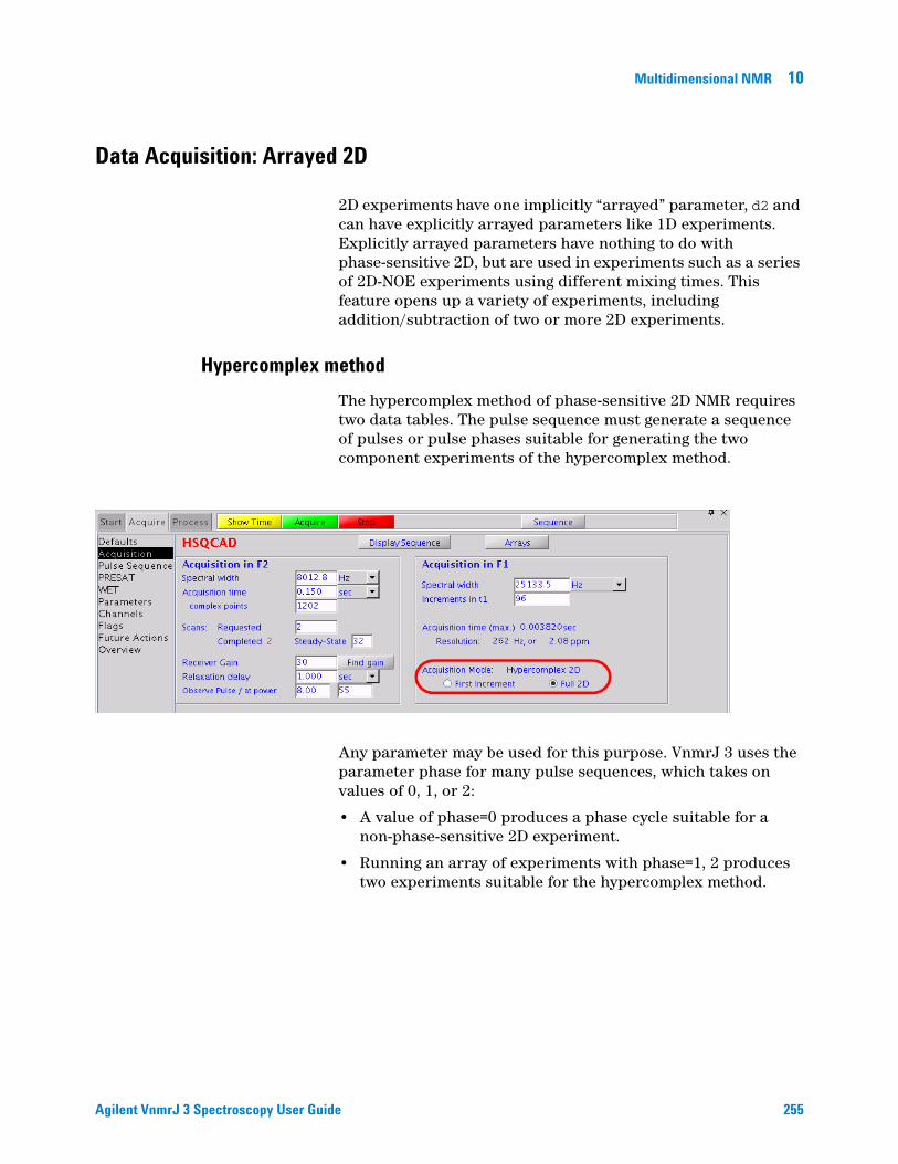
Multidimensional NMR 10
Data Acquisition: Arrayed 2D
Agilent VnmrJ 3 Spectroscopy User Gui
2D experiments have one implicitly “arrayed” parameter, d2 and can have explicitly arrayed parameters like 1D experiments. Explicitly arrayed parameters have nothing to do with phase-sensitive 2D, but are used in experiments such as a series of 2D-NOE experiments using different mixing times. This feature opens up a variety of experiments, including addition/subtraction of two or more 2D experiments.
Hypercomplex method
The hypercomplex method of phase-sensitive 2D NMR requires two data tables. The pulse sequence must generate a sequence of pulses or pulse phases suitable for generating the two component experiments of the hypercomplex method.
Any parameter may be used for this purpose. VnmrJ 3 uses the parameter phase for many pulse sequences, which takes on values of 0, 1, or 2:
• A value of phase=0 produces a phase cycle suitable for a non-phase-sensitive 2D experiment.
• Running an array of experiments with phase=1, 2 produces two experiments suitable for the hypercomplex method.
de 255

10 Multidimensional NMR
TPPI Method
256
The TPPI method of phase-sensitive 2D NMR requires one data table. The data is processed along t1 with a complex Fourier transform by setting proc1 (which sets the type of data processing to be performed on the t1 interferogram) to 'ft'. This manner of implementing TPPI leads to a doubling of the f1 frequency axis.
When an arrayed 2D experiment is run in this manner, there is in reality a double array: d2 (the evolution time) and phase. The order of these arrays is such that the phase array is cycled the most rapidly. Observe the order of these experiments; for example:
Not all pulse sequences have the TPPI method incorporated. The acquisition status window displays a count of the current FID and the number of completed transients (ct) in that FID. The current FID number is the total count of completed FIDs to this point, including all arrays. As the phase parameter is cycling the most rapidly, and since, typically, phase is an array of two values, the current FID number is typically twice the number of the current increment. For example, when the counter reads FID 54, this means that 27 FIDs of the first type of experiment have been completed, 26 of the second type, and the system is working on the 27th experiment of the second type.
Method Evolutiontime Phase
States-Haberkorn d2=0 phase=1
d2=0 phase=2
d2=1/sw1 phase=1
d2=1/sw1 phase=2
TPPI (non-arrayed) d2=0 phase=3
d2=1/sw1 phase=3
d2=2/sw1 phase=3
d2=3/sw1 phase=3
Agilent VnmrJ 3 Spectroscopy User Guide

Multidimensional NMR 10
Weighting
Agilent VnmrJ 3 Spectroscopy User Gui
This section describes weighting functions for processing 2D experiments.
2D weighting parameters
The 2D weighting parameters used for processing the t1 domain (the interferogram) or first indirectly detected dimension (ni) are set on the Process page in the Process panel and are analogous to weighting parameters for 1D experiments.
Non-phase-sensitive (absolute-value and power) 2D experiment
“Pseudo-echo,” sinebell, or sinebell-squared weighting is typically used to attenuate long dispersion tails. This weighting is often responsible for a significant loss in sensitivity in absolute-value 2D experiments.
Phase-sensitive 2D experiments
The key to using weighting functions is to use them to ensure that the weighted FID or interferogram decays to zero by the end to avoid “truncation wiggles.” The Gaussian function is ideally suited for this, typical values might be gf=0.6*at, gf1=0.6*ni/sw1 (=0.6*at1), which are entered in the Weight Parameters fields. Resolution enhancement (using negative line
Weighting AutoSelect weighting button
pseudo-echo Pseudo
sinebell Sine
sinebell-squared sq-sine
de 257

258
10 Multidimensional NMR
broadening) may be helpful in cases of spectral overlap, but can also be dangerous, since the “wiggles” that it can produce around the sides of peaks show up as peaks of opposite sign in the 2D plot, which complicates the analysis of the spectrum.
Interactive weighting
The Interactive Weighting button that shows up in several pages of the Process tab (or the wti command) allows interactive setting of the weighting parameters for any selected dimension (either the t2 FIDs or the t1 interferograms, for example, both the ni and ni2 dimension). The currently active element or trace is used in adjusting the weighting parameters.
Agilent VnmrJ 3 Spectroscopy User Guide

Multidimensional NMR 10
Agilent VnmrJ 3 Spectroscopy User Gui
The following graphics toolbar buttons control these parameters used with interactive weighting:
The values displayed in the graphics display window correspond to the values displayed in the Weight Parameters fields on the Process page. Clicking a graphics control button toggles the weighting function on and off.
Enter values in the fields next to the Weight Parameters and select the box to activate the parameter. Press Return to enter the value.
On the graphics screen, the left mouse button changes the selected parameters. The right mouse button turns the spectrum on and off. (This produces a faster response to changes in the weighting function, which was useful years ago on slower computers.)
1 pmode='' is both ph and ph1 must be executed before performing 2D FT.
• pmode='partial' is only ph must be executed before performing 2D FT.
• pmode='full' is a command must be executed before 2D FT.
Check Box Icon Function
Line broadening Selects line broadening or exponential weighting. A negative value gives resolution enhancement.
Sinebell Selects the sinebell constant. A negative value gives squared sinebell.
Shifted Sinebell Selects the sinebell shift constant (if sinebell is active)
Gaussian Selects the Gaussian time constant
Shifted Gaussian Selects the Gaussian shift constant (if Gaussian is active)
Additive weighting Selects the additive weighting constant
Return Returns to the previous menu
de 259

10 Multidimensional NMR
Baseline and Drift Correction
260
Use the Linear Prediction and Display pages in the Process tab to correct baseline and drift.
Calculating the preacquisition delay
Unless the first-order phase in the directly-detected dimension is approximately zero (which it should normally be on modern spectrometers), the non-zero lp value will affect both the spectral drift correction (dc) offset and the curvature of the spectrum during 2D data processing. Delay values are shown on the Acquire / Flags page. The ideal first-order phase correction should be close to zero. If the probe file is calibrated properly, this will occur automatically. If the probe files are not properly calibrated, do one of the following.
1 Enter setrc to calculate a new value for the ddrtc delay so that lp is rendered approximately 0 after acquisition. This is done before acquisition, and does not require an existing spectrum.
2 Enter setlp0 to calculate a new value for the ddrtc delay so that lp is rendered approximately 0 after acquisition. This macro requires an existing spectrum, properly phased (it looks at lp), and it must be followed by a reacquisition of the spectrum.
On older spectrometers, do one of the following:
1 Obtain a trial spectrum and phase it to pure absorption. This spectrum provides the current pre-acquisition delay and first-order phase values. Using these values, the calfa macro will calculate proper values for the pre-acquisition delays (like alfa) such that when the spectrum is re-acquired, lp should now be approximately 0 when the spectrum is properly rephased. This macro requires an existing spectrum, properly phased (it looks at lp), and it must be followed by a reacquisition of the spectrum.
2 Enter setlp0 to calculate a new value for the pre-acquisition delay (alfa) so that lp is rendered approximately 0 when the spectrum is reacquired. This macro requires an existing spectrum, properly phased (it looks at lp), and it must be followed by a reacquisition of the spectrum.
Agilent VnmrJ 3 Spectroscopy User Guide

Multidimensional NMR 10
Setting the receiver gating time
Agilent VnmrJ 3 Spectroscopy User Gui
Set the receiver gating time (typically rof2) to a value appropriate for the current probe and observe nucleus. On DDR systems (that is, VNMRS), the appropriate gating time for a cold probe is approximately 25 μsec to prevent ringing, and the appropriate gating time for a room temperature probe is approximately 25 μsec. On older spectrometers, the appropriate gating time for a cold probe is approximately 20 μsec, and the appropriate gating time for a room temperature probe is approximately 4 μsec.
First point multipliers
The fields under 1st Pt Multiplier (on the Linear Prediction page) multiply the first point of each FID by the F2 value and the first point of each interferogram (for the indirectly-detected dimension) by the F1 value. The 1st Pt Multiplier compensates for first point distortion in analog receivers (see Otting, Widmer, Wagner and Wuthrich, J. Magn. Reson. 1986, 66, 187). The default fpmult value on older spectrometers is 1.0, except if the processing involves backward extension of the time-domain data with linear prediction, in which case, the value is then 0.5. On newer spectrometers, the default fpmult value should always be 0.5. The default fpmult1 value is 0.5.
The effect of using the F2 value in 1st Pt Multiplier is to perform a linear baseline correction on all F2 data, reducing negative-going ridges along F2 in phase-sensitive 2D data. This correction is not needed in experiments such as COSY, where the FID starts at zero and grows. It is also not needed in absolute-value mode presentation, if pseudo-echo or sinebell processing is used, because the processing function goes to zero at t2=0, forcing all FIDs to start at zero amplitude.
Typically, no correction for 1st Pt Multiplier is necessary. Automatic empirical setting of fpmult is available through the macro cfpmult, which is used on a first increment spectrum. Clearing the check boxes next to F1 and F2 disables the first-point multiplier feature. This is the usual value for sinebell or pseudo-echo processing.
de 261

262
10 Multidimensional NMR
The best empirical value of the 1st Pt Multiplier can also be determined manually. It can be determined manually during or after the acquisition of the 2D data by using the FT 1D -1st Increment button in the Process pages.
1 Enter dc or use the DC Correct button with a properly phased first increment spectrum on the screen.
2 Position the mouse at the right edge of spectrum baseline (to keep track of the ideal baseline position).
3 Enter cdc and observe the new position of the baseline. It typically drops.
• Baseline goes negative: set the F2 1st Pt Multiplier to greater than 1.0 (try 1.5) and click FT 1D - 1st Increment on the Process / Default or Process / Display pages.
• Baseline rises but does not return to the position indicated by the mouse arrow: increase the value of F2 1st Pt Multiplier and click FT 1D - 1st Increment again. If in doing so the baseline rises above the ideal level, reduce the value and try again.
Usually, only a few tries are required before the proper value of F2 1st Pt Multiplier is found.
Spectral drift correction
Drift corrections can be performed on the 2D datasets as well. This can sometimes help remove ridges from the processed data. The DC Correct (F1, F2) button on the Process / Default page performs drift corrections along both axes, and should only be performed after the 2D transform. The drift corrections can also be called via the command line using dc2d('f2') and dc2d('f1'), in which case, they can be using either during or after the 2D transform, as long as the indicated axis has been transformed.
Agilent VnmrJ 3 Spectroscopy User Guide

Multidimensional NMR 10
Baseline correction
Agilent VnmrJ 3 Spectroscopy User Gui
Baseline Correction is related to the 1st Pt Multiplier and Drift Correction tools, which are used to remove ridges from the processed data. Access baseline correction on a 2D dataset by clicking on the BC Correct (F1, F2) button on the Process / Default page. It performs baseline corrections along both axes, and should only be performed after the 2D transform. Baseline correction in 2D processing uses the spline or second to twentieth order polynomial fitting of predefined baseline regions. These regions are set up prior to the use of bc by setting integral resets so that integrals appear only over regions of the spectrum with signals present. These can be set after clicking FT 1D - 1st Increment. The quality of the baseline correction can be assessed by bc(1). The baseline corrections can also be called via the command line using bc2d('f2') and bc2d('f1'), in which case they can be using either during or after the 2D transform, as long as the indicated axis has been transformed.
In setting baseline regions near the ends of the spectrum, the actions of the bc and dc operations are similar to the 1st Pt Multiplier, because they all represent a simple spectral drift correction.
de 263

10 Multidimensional NMR
Processing Phase-Sensitive 2D and 3D Data
264
The complete 2D transformation can be performed after 2D data has been acquired by using one of the Transform buttons on the Process pages. A typical example would be the Full 2D Transform button on the Process / Default page.
A series of complex FIDs, obtained as a function of t1, are transformed to become a series of spectra. Each spectrum contains a real and imaginary part. Each spectrum is then phase-rotated, according to the phase correction determined from an individual spectrum. This produces a series of spectra, each consisting of an absorptive and a dispersive part, formed as linear combinations of the original real and imaginary parts. Complex interferograms then form out of corresponding points along the frequency axis from each of the spectra and this is transformed to produce the final 2D spectrum.
The real and imaginary part of the interferograms can be formed from any linear combination of the real and imaginary parts of one or more spectral sets after the first Fourier transformation. Refer to these coefficients below according to the following scheme: RR1 is the coefficient used to multiply the real part (first R) of spectra in set 1 (the 1) before it is added to the real part (second R) of the interferogram. IR2 thus represents the contribution from the imaginary part of spectra in set 2 to the real part of the interferogram, and so on.
Another set of complex interferograms are formed from these two sets of F2 spectra for some experiments. This set of interferograms is 90° out-of-phase in F2 to the previous set and can be constructed without any additional coefficients.
Different experiments require different coefficients. Some, such as heteronuclear 2D-J experiments, consist of only one FID and spectral set, and hence need a total of four coefficients to be processed correctly. Others, including hypercomplex 2D experiments, consist of two original data sets and need a total of eight coefficients to allow it to be processed correctly. Other experiments are possible with three or even more data sets, requiring in each case, four times as many coefficients as the number of data sets (see the macro wft2dac).
4n coefficients must be supplied if there are n data sets to be transformed, as in typical phase-sensitive experiments. The first 2n coefficients are the contributions to the real part of the interferogram, alternating between real and imaginary parts of the successive data sets. The next 2n coefficients are the contributions to the imaginary part of the interferogram, in the same order.
Agilent VnmrJ 3 Spectroscopy User Guide

Multidimensional NMR 10
Agilent VnmrJ 3 Spectroscopy User Gui
Thus, using the definition that the first letter refers to the source data set, the second letter refers to the interferogram, and the number identifies the source data set, we have the cases shown in the table.
The coefficients are generally 1, 0, or –1, but other coefficients are acceptable. Any real coefficient can be used, and as many coefficients can be non-zero as is desired. Up to 32 coefficients can be supplied, which at four per data set, allow the addition, subtraction, etc., of eight 2D data sets (that is, eight different phase cycles). See the macro wft2dac for more information.
Data Sets Coefficient Order
1 RR1, IR1, RI1, II1.
2 RR1, IR1, RR2, IR2, RI1, II1, RI2, II2.
3 RR1, IR1, RR2, IR2, RR3, IR3, RI1, II1, RI2, II2, RI3, II3.
... ...
Processing programs
A number of processing programs are available:
• ft1d(coefficients) performs only the first Fourier transformation along the F2 dimension (without weighting) and matrix transposition, allowing the display of interferograms with the wti, dcon, and dconi commands.
• wft1d(coefficients) functions the same as ft1d except weighting is included.
• ft2d<(<option,>coefficients)> performs a complete transformation in 2D, without weighting, after 2D data has been acquired. If the first Fourier transformation has already been done using ft1d, wft1d, ft1da, or wft1da, then ft2d performs only the second (t1) transform. 'ptype' or 'ntype' can be used as the first argument to select P-type or N-type peak selection. The coefficients arguments are discussed below.
• wft2d<(<option,>coefficients)> performs the same as ft2d, except weighting is included. To perform a normal 2D transform on the n-th element in an arrayed 2D experiment, type wft2d(n).
de 265

266
10 Multidimensional NMR
• ft2da<('bc',polynomial_order)> runs complete phase-sensitive Fourier transform after the 2D FID data has been acquired. 'bc' is a keyword to perform a baseline correction on the F2 spectra prior to the Fourier transform along F1. The polynomial_order is the order of the polynomial used in the baseline correction.
• wft2da<('bc',polynomial_order)> functions the same as ft2da, except weighting is included.
• ft1da functions the same as ft2da, except a Fourier transform along F1 is omitted.
• wft1da functions the same as ft1da, except weighting is included.
You can reduce the processing time for some 2D data sets by selectively transforming the t1 interferograms. The command ft2d('f2sel') allows only preselected F2 regions to be transformed along t1; the t1 interferograms in the non-selected F2 regions are zeroed but not transformed. The same mechanism that is used to select baseline regions for baseline correction (bc) is used to select the F2 regions that are to be transformed along t1. Partition the integral of the spectrum into several regions. The even numbered F2 regions, for example, 2, 4, etc., will be transformed along t1; the odd numbered ones will not be transformed along t1.
Unreliable peak heights can be caused by Fourier transformation of truncated time-domain data. To obtain properly defined signals, take one of the following steps:
• Collect data until the signal has decayed to zero in the time domain.
• Transform the data with zero-filling (fn>=2*np, fn1>=4*ni).
Taking one of these steps is particularly important in 2D spectra with antiphase or dispersive signals, where underdigitization can lead to signal cancellation.
Common coefficients for wft2d processing
To enter process coefficients, use the Transform Coefficients field on the Process/Default page. Typically, the coefficients are already set in the 2D parameter sets (4 coefficients for absolute value mode and 8 coefficients for phase-sensitive).
A magnitude-mode transform, in which the real part of the interferogram is formed from the real part of the spectra and the imaginary part of the interferogram is formed from the imaginary part, would require 1,0,0,1. Changing the sign of
Agilent VnmrJ 3 Spectroscopy User Guide

Multidimensional NMR 10
Agilent VnmrJ 3 Spectroscopy User Gui
the imaginary part of the interferogram serves to change the effective direction of the F1 frequency axis, as is required for data in which N-type peaks are detected. This can be done with 1,0,0,-1.
In some experiments, including heteronuclear 2D-J, the basic data are purely amplitude modulated, with a starting amplitude of +1. After the first transformation and phasing operation are complete, the dispersion part of each spectrum serves only to produce a phase-twist in the final spectrum without contributing any information. Setting the imaginary part of the second transform to zero produces a pure absorption display in both domains: 1,0,0,0.
In the hypercomplex method of acquiring pure absorption 2D data, we have two complete sets of spectra and must therefore provide eight coefficients to specify the composition of the interferograms. A typical execution of the method described by States, Haberkorn, and Ruben, assuming that the first spectrum of the first data block has been phased for absorption, requires 1,0,0,0,0,0,1,0 to produce pure absorption spectra.
Other manipulations of two data blocks are formatted similarly. A magnitude-mode 2D experiment that is the sum of the two different experiments can be constructed by 1,0,1,0,0,1,0,1. For a COSY experiment, this would produce the P-type experiment. Subtracting data block two from block one, which for a COSY experiment gives the N-type COSY, would be accomplished by 1,0,-1,0,0,1,0,-1. Thus, two different absolute-value 2D experiments, (P-type and N-type) and a phase-sensitive 2D experiment, can be produced from the same data set, without acquiring the data again.
Different combinations of data sets with appropriate phase cycling might allow selection of various quantum orders in a single experiment. Note that since the coefficients may be different from one, it is possible essentially to phase shift each experiment separately (phase shift the receiver) after the experiment is done. For TPPI data with phase=3, only one data set is collected, and the imaginary part of the second transform is set to zero: 1,0,0,0.
The parameter f1coef is used to store the above coefficients as text strings and is displayed under the label Transform Coefficients.
de 267

10 Multidimensional NMR
2D solvent subtraction filtering
268
2D solvent subtraction is set up on the Process / Linear Prediction page. In a 2D transform, solvent subtraction is invoked on t2 FIDs. The parameters ssfilter and ssorder select the processing option as follows:
• The zfs (zero-frequency suppression) option is selected if both bandwidth (ssfilter) and polynomial (ssorder) are set to a value.
• The lfs (low-frequency suppression) option is selected if bandwidth is set to a value and polynomial is not selected.
• The solvent subtraction (both the zfs and lfs options) is turned off if the bandwidth is blank.
Left shift FID, left shift frequency, phase rotation
Use the Process / Linear Prediction page to adjust the Left Shift FID, Left Shift Frequency, and the Phase Rotation.
Check Left Shift FID to left-shift the FID by the entered number of complex (or hypercomplex) points before the weighting and Fourier transformation are performed. The parameter name is lsfid; the value must be between 0 and np minus 1.
Enter a negative value for Left Shift Frequency to shift the peaks upfield (to the right) or a positive value to shift the peaks downfield (to the left). The Left Shift Frequency (lsfrq) operates only on the F2 data. Arelated parameter (lsfrq1) performs a similar function in F1.
Apply a phase-rotation to the interferogram by checking the appropriate box and entering a value in degrees (zero-order phase rotation). This causes zero-order phase rotation before weighting and Fourier transformation are performed.
Agilent VnmrJ 3 Spectroscopy User Guide

Multidimensional NMR 10
2D processing of 3D data
Agilent VnmrJ 3 Spectroscopy User Gui
Acquisition and full processing of 3D data requires the parameters ni2 and sw2 (d3 is the delay increment in the ni2 dimension). 2D processing of “slices” of the 3D data matrix is accomplished using the following commands:
ft2d('ni2') Transforms non-arrayed 2D data that have been collected with ni2 and sw2 (instead of ni and sw1). The addpar('3d') macro creates the necessary processing parameters for the ft2d('ni2') operation (par3d functions the same as addpar('3rf')).
ft2d('ni',#) Selectively transforms selected np-ni 2D plane within a non-arrayed 3D data set, # is an integer that can range from 1 to ni2.
ft2d('ni2',#) Selectively transforms selected np-ni2 2D plane within a non-arrayed 3D data set, # is an integer that can range from 1 to ni.
wft2d Acts the same as ft2d, but applies weighting before transformation.
The format of the arguments to ft2d changes if an arrayed 3D data set is selectively processed. For example, ft2d('ni',#1,#2) performs a 2D transform along np and ni of the #2-th ni2 increment and the #1-th element within the explicit array. This yields a 2D np–ni frequency plane. #1 ranges from 1 to ni2; #2 ranges from 1 to [arraydim/(ni*ni2)].
Arrayed 3D data sets can also be subjected to 2D processing to yield 2D absorptive spectra. If the States-Haberkorn method is used along both F1 (ni2 dimension) and F2 (ni dimension), there will generally be four spectra per (ni,ni2) 3D element. In this case, the command ft2d('ni2',#1,<16 coefficients>) performs a 2D transform along np and ni2 of the #1-th ni increment using the ensuing 16 coefficients to construct the 2D t1-interferogram from appropriate combinations of the four spectra per (ni,ni2) 3D element. Use the proc2 parameter to specify the type of data processing to be performed on the ni2 interferogram (3D): 'ft' for complex FT, 'rft' for real FT, or 'lp' for linear prediction processing on complex data. The macro dg2 displays 3D processing parameters in the test output page.
de 269

10 Multidimensional NMR
2D and 3D Linear Prediction
270
Linear prediction parameters are adjusted on the Linear Prediction page. The F1 check box controls the transformation process along t1, and the F2 check box controls the transformation process along t2. Using the same method of transformation is not necessary along two (or three axes). For example, you can employ a backwards linear prediction in t2 of a 2D experiment and a forward linear prediction along t1, or perhaps a simple Fourier transformation along t2 and a backwards linear prediction along t1.
Agilent VnmrJ 3 Spectroscopy User Guide

Multidimensional NMR 10
Phasing the 2D Spectrum (Both F1 and F2)
Agilent VnmrJ 3 Spectroscopy User Gui
The phase constants lp1 and rp1 control the phase correction along F1 in phase-sensitive data. These should ideally be near zero in most 2D experiments. Finite pulse widths and delays in the pulse sequence can cause deviations from zero, but standard pulse sequences should properly compensate for these imperfections and make it possible to have zero lp1 and rp1. Most of the setup macros set lp1 and rp1 to zero so that the first display of the 2D spectrum will indicate the need (if any) for phase correction in F1. The same techniques as used in 1D phasing are employed here, with minor differences. (The methodology listed below can also be used to phase F2 if appropriate modifications are made.)
1 Enter f full to display the full data matrix in a full chart display.
2 Phase the 2D spectrum: Use the horizontal cursor in the interactive display to identify a peak toward the right-hand edge of the spectrum. Note the trace number indicated at the top of the display (“memorize” this by setting r1 equal to its value.)
3 Select one or more other traces at F1 values more toward the center and left parts of the spectrum. (One easy option for spectra with a large diagonal is to use peaks on the diagonal. These will typically provide very sensitive phase corrections.) Use r2, r3, etc. to “memorize” these trace values. A minimum of two is needed, one at the far right and one at the far left.
4 Enter ds(r1). Phase this spectrum like a 1D spectrum (for example, by using the Phase button in the graphical toolbar). Click the mouse on the peak displayed near the right edge of the spectrum. Phase up this spectrum (thus setting rp1). Do not click in the left part of the spectrum at this time.
5 Enter ds(r2). The second trace appears. Click the mouse near the right edge of the spectrum (to fix rp1 at the previously determined value) and do not rephase. Move the mouse to the peak at the left, click and phase it (thus setting lp1).
6 Enter ds(r1) to recheck rp1. Repeat the process again if necessary.
Use the diagonal peaks for phasing in homonuclear correlation spectra (such as NOESY, TOCSY, and ROESY). Phase an f1 trace exactly like a 1D spectrum if there are strong cross-peaks. Phase HMQC spectra by progressively working from right to left, with
de 271

272
10 Multidimensional NMR
several peaks selected along the way to make sure that lp1 does not go through an extra revolution that would induce some baseline roll.
Corrections in f2 phasing may be obvious in the 2D data when they are not in the first increment 1D spectrum. If pmode='full' before the 2D transform, f2 phasing may be corrected without retransforming by setting trace='f2' and using the same approach as described for f1phasing. Transformation of the data again is necessary if pmode='' or pmode='partial'. No f1 phasing is possible after transformation if pmode=''. f1 phasing after the transform is possible (but not f2 rephasing) if pmode='partial'. Do baseline corrections such as dc2d or bc only after data is properly phased in f1 and f2.
Agilent VnmrJ 3 Spectroscopy User Guide

Multidimensional NMR 10
Display and Plotting
Agilent VnmrJ 3 Spectroscopy User Gui
This section discusses the manual mode of (non-interactive) 2D display and plotting. For more details, see Chapter 8, “Printing, Plotting, and Data Output” .
Display modes
Select display modes in the Display page.
Display and plot limitsThe center, left, right, and full set the spectrum to display (and subsequent plot) in the relevant portion of the screen (and page).
Display scaling
The peak2d command searches the area defined by sp, wp, sp1, and wp1 in a 2D data set for a maximum intensity. It returns the maximum intensity value found, the trace number of the maximum, and the data point number of the maximum on that trace.
The AutoScale 2D button on the Display page uses peak2d to set up the vertical scaling and threshold for a 2D contour plot and color map display.
de 273

10 Multidimensional NMR
Grid lines
274
A grid of horizontal and vertical lines over a 2D display can be drawn by the grid macro. By default, grid lines are drawn in blue at approximately 1 cm intervals, rounded so that the intervals fall at a multiple of 1, 2, or 5 Hz or ppm. To change the defaults, enter grid with a different spacing (in cm) or a different color ('red', 'green', etc.); for example, grid(2,'white') gives white grid lines at 2 cm intervals.
The grid command also can define a grid, using the following syntax:
grid<(startf2,incrf2,startf1,incrf1,color)>
The arguments define the frequency and increments between grid lines in the f2 and f1 directions and the color of the grid lines.
The plgrid macro uses the same arguments as grid, but plots the grid instead.
Whitewashed spectra
The dsww<(start,finish,step)> command displays one or more spectra with whitewashing (traces in front “block” the view of traces behind them). Use the argument 'all' to display all spectra. plww<(start,finish,step)> plots the same spectra.
Use the Stacked Plot graphics button in the Plot page to display a stacked display of 2D spectra in the whitewash mode.
Agilent VnmrJ 3 Spectroscopy User Guide

Multidimensional NMR 10
Label display
Agilent VnmrJ 3 Spectroscopy User Gui
The dssl macro displays a label for each element in a set of stacked spectra. The label is an integer value starting with 1 and ranging to the number of spectra in the display.
Labels can appear at incorrect positions if wysiwyg='n'. The positions were empirically determined for a large screen display and are not guaranteed to be correct for all displays.
The following options control the dssl display (more than one option can be entered as long as the options do not conflict with each other):
• 'center', 'left', 'right', 'top', 'bottom', 'above', and 'below' are keywords setting the position of the displayed index relative to each spectrum.
• 'value' is a keyword that produces a display of the values of each array element, instead of an integer index.
• 'list=xxx' produces a display of the values contained in the arrayed parameter xxx.
• 'format=yyy' uses the format yyy to control the display of each label. See the write command for information about formats.
2D referencing
Use the Referencing buttons on the Process / Display page to modify (as needed) the referencing of 2D spectra.
Enter a frequency (in Hz or PPM) to re-reference the indicated chemical shift axis.
Click the Cancel button to reset referencing along F2 and F1.
de 275

276
10 Multidimensional NMR
Use the centersw macro to indicate the center of the directly detected dimension, and the centersw1 macro to indicate the center of the first indirect dimension. Use both to center the cursors in the spectrum.
Prior to acquisition, you can use the macro setsw1(nucleus,downfieldppm,upfieldppm) to set the spectral width to a given spectral window.
Rotating homonuclear 2D-J spectra
The rotate command rotates homonuclear 2D-J data 45° (rotation in frequency-space) to line up multiplets. Use the rotate(angle) command with the angle argument to specify other angles.
Setting negative intensities to zero
The command zeroneg is used for the projection of proton 2D-J spectra at 45° to strip a high-resolution proton spectrum down to a list of chemical shifts. The zeroneg command sets all negative intensities to zero.
Agilent VnmrJ 3 Spectroscopy User Guide

Multidimensional NMR 10
Interactive 2D Color Map Display
Agilent VnmrJ 3 Spectroscopy User Gui
Use the graphics control buttons and the mouse to control the display in the graphics window.
2D display
Below is an example of a 2D display with the projection graphics control buttons selected.
Controls for adjusting the color/grayscale are on the right side of the window.
The interactive display parameters are displayed across the bottom of the graphics window (assuming "fields" is checked "on" in the Frame vertical panel):a
cr Shows the current cursor position
cr1 Shows the current cursor position along the first indirectly detected dimension
delta Shows the cursor difference
delta1 Shows the cursor difference along the first indirectly detected dimension
vs2d Shows the vertical scale of the display
vsproj Shows the vertical scale of the trace or projection
de 277

10 Multidimensional NMR
Interactive nD display control buttons
278
Table 17 Main nD display bar tools
Icon Description
Display color map and show common nD graphics tools
Display contour map and show common nD graphics tools
Display stacked spectra and show common nD graphics tools
Display image map and show common nD graphics tools
Table 18 nD graphic tools
Icon Description
One cursor in use, click to toggle to two cursors
Two cursors in use, click to toggle to one cursor
Click to expand to full display
Pan and stretch
Show trace
Show projections
Click to show horizontal maximum projection across the top of the 2D display
Click to show horizontal sum projection across the top of the 2D display
Click to show vertical maximum projection down the left side of the 2D display
Click to show vertical sum projection down the left side of the 2D display
Rotate axes
Increase vertical scale 20%
Decrease vertical scale 20%
Agilent VnmrJ 3 Spectroscopy User Guide
Multidimensional NMR 10
Agilent VnmrJ 3 Spectroscopy User Gui
Phase spectrum
Click to select the first spectrum
Click to select the second spectrum
Enter peak pick menu
Table 18 nD graphic tools (continued)
Icon Description
Cursors
Use the left and right mouse buttons to move cursors, and the center button to adjust the vertical scale of traces, projections, and contour maps, as well as to adjust the threshold in the optional color bar. The cursors can be used to select regions for expansions of the display. The cursors can also be used to select positions to “mark” using the ll2d('mark') command, which displays and records spectral frequencies, maxima, intensities, and volumes.
The left mouse button adjusts the position of the 2D cursor. The corresponding frequencies are displayed at the bottom of the graphics window. Both the horizontal and vertical cursors move if the left mouse button is pressed within the 2D display box.
Above and below the box, only the vertical cursor can be moved. At the left and the right of the box, only the horizontal cursor can be moved. In addition, holding the mouse button down and then moving the mouse moves the cursor with the mouse.
The function of the center mouse button depends on the location of the cursor:
• Cursor is within the 2D display box: In gray scale images, pressing the center button sets the point to medium gray. Otherwise, for color map and contour displays, if there is no intensity at that point, the center button changes vertical scale to show intensity at that point. If there is intensity at the point, the center button changes the scale to show no intensity, then changes the parameter vs and redraws.
• Cursor is near an active trace and active horizontal or vertical projection: Pressing the center button changes the vertical scale of trace or projection, so that the spectrum goes through the current mouse position.
de 279

280
10 Multidimensional NMR
• Cursor is near the color/grayscale bar and in the color mode: Pressing the center button sets the threshold to remove low intensity peaks. If in the grayscale mode, pressing the center button sets the grayscale intensity (the right button adjusts contrast).
A second cursor pair is displayed with the right mouse button. The second pair can be moved in exactly the same way as the first pair, and is used to select a box within the 2D display. The right mouse button also switches the display into the box mode, the same as clicking on the Box button in the menu.
Traces
1 Click the Trace icon. A trace is displayed for the position of the horizontal cursor.
2 Move the horizontal cursor to change the displayed trace.
3 Adjust the vertical scale of the trace by clicking the middle mouse button on the trace, not in the 2D spectrum.
Exit the trace mode by displaying a box with the right mouse button, or by selecting another display mode.
Projections
1 Click the Projection icon to open the Projection graphic control buttons.
2 Select the type of direction (horizontal or vertical) and mode (maximum or summary).
3 Adjust the vertical scale of the projections with the middle mouse button.
Expanding the display
1 Use the Box cursors to select the region in the spectrum to expand.
2 Click the Expand icon to obtain an expanded display.
Setting the vertical scale
If a peak is expected at a certain position in the spectrum but is not visible, click once at that position with the middle mouse button. This selects a new vertical scale, so that the intensity at that point is by a factor of 2 above the threshold, and the display is redrawn.
Agilent VnmrJ 3 Spectroscopy User Guide

Multidimensional NMR 10
Adjusting the threshold
Agilent VnmrJ 3 Spectroscopy User Gui
If noise is visible at a certain position in a spectrum, but should be suppressed below the threshold, click once at that position with the middle mouse button. A vertical scale is calculated so that this intensity falls by a factor of 2 below the threshold, and again the spectrum is redrawn.
Treating 2D traces as 1D spectra
Enter the command ds after a trace has been selected in the interactive 2D display program to allow the trace to be displayed as if it were a simple 1D spectrum. All standard 1D data manipulations, including line listing, integration, etc., are then accessible for that trace. The command ds(tracenumber) can also be used to display an F1 or F2 trace, depending on the value of trace.
de 281

10 Multidimensional NMR
Interactive 2D Peak Picking
282
The ll2d program is used to automatically or interactively pick peaks in 2D spectra or 2D planes of 3D spectra. The peaks can be displayed on top of the spectrum in the dconi display or can be plotted using the pll2d command.
The results of all peak-picking operations are stored in a binary file in the ll2d subdirectory of the current experiment directory:
• The results are stored in the file peaks.bin for 2D spectra.
• The results are stored in peaks_f#f#_#.bin for 2D planes of 3D spectra, where f#f# denotes the orientation of the plane being picked (for example, f1f3 or f2f3), and the last # denotes the number of the plane.
Binary peak files can be converted to text files for printing or for export to other programs.
For each peak in a peak file, the following information is stored:
• Peak number
• Interpolated peak frequency in both dimensions
• Interpolated peak amplitude
• Full width at half-height (FWHH) in both dimensions
• Bounds of the peak in both dimensions
• Volume of the peak
• 15-character peak label
• 80-character comment
Agilent VnmrJ 3 Spectroscopy User Guide

Multidimensional NMR 10
Interactive 2D peak picking buttons
Agilent VnmrJ 3 Spectroscopy User Gui
Most of the above options are accessible through a series of graphics control buttons. From the 2D Display, the Peak Picking button brings up the 2D Peak Picking buttons.
Return
Display
File
Edit
Auto
Peak PickingMain Menu
AutomaticPeak Picking
Box/Cursor
Expand/Full
Auto Peak Pick
Auto Pick Footprints
Auto Pick Peak and FootprintsAdjust for overlap
Delete all peak picks
EditPeaks
Box/Cursor
Expand/Full
Pick peaks
Un-pick peaks
Delete all peak picksCombine peak picks
Display info - nearest peak
Integrate 2D peaks
Peak Files
Read Binary Peak Pick File
Read Peak Pick Text File
Write Peak Pick Text FileWrite Binary Peak Pick File
Display Peaks
Show Peak Picks
Show Peak Pick Numbers
Show FootprintsShow Peak Labels
Show All Peak Markers
Hide All Peak Markers
Return
Return
Return
Return
These buttons provide access to the following menus (depending on the mode, the labels on some buttons change).
The following menu selects another 2D Peak Picking menu. The buttons function as follows:
Table 19 2D peak picking main menu
Auto Displays the buttons for automatically picking peaks.
Edit Displays the buttons for interactively editing peaks.
File Displays the buttons for manipulating peak files.
Display Displays the buttons for controlling the display of peaks.
Return Returns to the 2D Color Map Display buttons.
de 283

284
10 Multidimensional NMR
This menu provides automatic peak picking. The buttons functions as follows:
Table 20 2D peak picking automatic menu
Box/ Cursor Selects the cursor mode.
Expand/ Full Selects expanded or full display.
Peak Automatically finds peaks in the 2D spectrum. If one cursor is visible, all peaks above the current threshold in the currently displayed region of the spectrum are found and marked. A peak is defined as a data point that is higher than the eight points around it. Once such a point is found, the actual peak location is determined by interpolation in both dimensions.
Volume Automatically finds the bounds of a peak and the integral of all points within these bounds. The bounds are found by descending down the sides of a peak until the point is reached where the amplitude of a data point is less than th2d times the current threshold. Thus, using a smaller value for th2d will cause ll2d to find and integrate a larger area for the bounds of the peaks. The peak volume is calculated by summation of all data points within these bounds. If the bounds of a peak already exist, the volume is recalculated.
Both Picks peaks and calculates volumes. The Both button does both the peak and volume operations at once.
Adjust Adjusts peak bounds so that none overlap. The Adjust button adjusts all peak bounds in the displayed region of the spectrum so that none overlap and recalculates peak volumes with the new peak bounds.
Reset Deletes all peaks that have been found in the current spectrum.
Return Displays the 2D Peak Picking buttons.
This menu provides interactive peak editing. The buttons functions as follows:
Table 21 2D peak picking edit menu
Box/ Cursor Selects cursor mode.
Expand/ Full Selects expanded or full display.
Mark In dconi cursor mode, this button inserts a peak at the current cursor location. In dconi box mode, the cursors are taken as peak bounds, and the area inside the cursors is integrated. These peak bounds are then assigned to all peaks within the cursors that do not already have their bounds defined. If a peak without bounds does not exist inside the area defined by the cursors, the highest point within that area is found, marked as a peak, and assigned the bounds defined by the cursors.
Unmark In dconi cursor mode, this button deletes the peak nearest the cursor. In dconi box mode, this button deletes peak bounds from peaks whose bounds are entirely within the area defined by the cursors.
Clear In dconi cursor mode, this button deletes all peaks in the area of the spectrum displayed in dconi. In dconi box mode, the Clear button deletes all peaks that are within the area defined by the cursors.
Agilent VnmrJ 3 Spectroscopy User Guide

Multidimensional NMR 10
Combine This button works only in dconi box mode. It combines all peaks within the area defined by the cursors into a single peak. This combination peak is located at the average frequencies of all of the original peaks and has bounds that encompass all of the original bounds of the peaks. The volume of the combination peak is calculated by summation of all data points within its bounds. Use the Backup File button in the 2D Peak Picking File menu (see below) prior to using the Combine button to save the original peaks if this data must be kept. Crating the combination peak are permanently deletes the contents of the current file.
Label Prompts for a 15-character label to be assigned to the peak nearest the cursor (dconi cursor mode) or to all peaks within the area defined by the cursors (dconi box mode). Based on the value of the parameter ll2dmode, this label can be displayed next to the peak in dconi.
Comment Prompts for an 80-character string to be assigned to the peak nearest the cursor (cursor mode) or to all peaks within the area defined by the cursors (box mode).
Info Prints the peak file information about the peak nearest the cursor to the text window.
Set Int Sets the value of the peak volume.
Return Displays the 2D Peak Picking main menu. (See Table 19 on page 283).
Table 22 2D peak picking file menu
Read Prompts for the filename of a binary peak file and reads that file into VnmrJ 3. When a file is read in, the current peak file (peaks.bin for 2D spectra) is overwritten by a copy of the peak file that was read in.
Read Text Prompts for the file name of a text peak file and reads that file into VnmrJ 3. When a file is read in, the current peak file (peaks.bin for 2D spectra) is overwritten by a new binary copy of the peak file that was read in.
Write Text Prompts for a filename to write a text version of the current ll2d peak file.
Backup File Prompts for a file name to copy the current binary peak file. Do this occasionally when doing a significant amount of interactive peak editing, so that intermediate versions of the peak file can be recovered in the event of an error (such as inadvertently selecting the Clear or Reset button or making a mistake using the Combine button).
Return Displays the 2D Peak Picking main menu. (See Table 19 on page 283).
Table 23 2D peak picking display menu
Show Peak/ Hide Peak
Show Peak: The “+” is hidden and this button shows a “+” at the location of each peak.Hide Peak: The “+” is shown and this button hides the “+” at the location of each peak.
Show Num/ Hide Num
Show Num: The peak numbers are now hidden, and this button shows a peak number next to each peak.Hide Num: The peak numbers are now shown, and this button hides the peak numbers.
Show Box/ Hide Box
Show Box: The box is now hidden, and this button shows a box with the area integrated to get the volume of the peak.Hide Box: The box is now shown, and this button hides this box.
Table 21 2D peak picking edit menu (continued)
Agilent VnmrJ 3 Spectroscopy User Guide 285

10 Multidimensional NMR
Show Label/ Hide Label
Show Label: The peak labels are now hidden, and this button shows a peak label next to each peak.Hide Label: The peak labels are now shown, and this button hides peak labels.
Show All/ Hide All
Show All: Displays a “+”, the peak number, the peak bounds, and the peak label for each peak.Hide All: Hides all peak information.
Return Displays the 2D Peak Picking button.
Table 23 2D peak picking display menu (continued)
286 Agilent VnmrJ 3 Spectroscopy User Guide

Multidimensional NMR 10
3D NMR
Agilent VnmrJ 3 Spectroscopy User Gui
VnmrJ 3 includes full support for 3D NMR, including acquisition, processing, and display.
Many of the 3D-related macros and parameters—for example, centersw2, cr2, crl2, delta2, dmg2, lp2, lsfid2, phfid2, rfl2, rfp2, rp2, sp2, wp2—are normally used in the same manner as their 1D and 2D counterparts and are not described further in this section.
A non-arrayed 3D experiment has two implicitly arrayed parameters: d2 and d3. d2 is associated with ni and sw1, d3 with ni2 and sw2. The order of these two arrayed parameters is such that d2 is normally cycled the most rapidly.
An arrayed 3D experiment, such as a single 3D with “superhypercomplex” data acquisition (States-Haberkorn method applied along both t1 and t2), has at least three arrayed elements. By convention, such an arrayed 3D experiment is implemented using four arrayed elements: d3 (t2 evolution time), phase2, d2 (t1 evolution time), and phase. Assuming that array='phase,phase2' (see below), the order of arrays is such that the phase2 array is cycled the most rapidly, followed by the phase, d2, and d3 arrays.
3D acquisition
3D data acquisition is accomplished with pulse sequences using the parameter d3, which is updated according to the parameters ni2 and sw2. This is analogous to incrementing d2 according to ni and sw1 for 2D NMR (of course, d2, ni, and sw1 are active in 3D as well). In addition, the parameter phase2 is used to control the “mode” of acquisition (hypercomplex, TPPI, or absolute value) in the third frequency domain, just like phase in the second domain. All of these 3D parameters are created with the macro addpar('3d') along with other 3D parameters, including fiddc3d for 3D time-domain dc correction, ptspec3d for region-selective 3D processing, and path3d for the path to the currently displayed 2D planes extracted from a 3D data set. (The macro par3d is functionally equivalent to addpar('3d').)
By convention, 3D sequences are described with the first evolution time being known as t1, the second evolution time as t2, and the time during which data are acquired as t3. After transformation, these same dimensions are called the F1, F2, and F3 dimensions.
de 287

10 Multidimensional NMR
3D processing
288
Data processing includes the ft3d command for full 3D processing, governed by the usual parameters to control transform sizes, weighting, phasing, etc., with a “2” at the end of the parameter name signifying the third dimension. Unlike other commands, ft3d occurs in the background by default. That is, it is run as a separate task, leaving VnmrJ 3 free to continue with other tasks (including 1D and 2D processing of the same data set). To increase the speed of 3D transforms further, the wftt3 macro allows the software to process one dimension (the acquisition or t3 dimension) as the data are being acquired. Also, the ft3d software can be configured to run on several computers simultaneously, for even greater speeds. The killft3d macro terminates any ft3d program that has been started in an experiment.
3D display
Display the data as two-dimensional planes of the 3D data set in any of the three orthogonal directions. Skew planes are not supported, nor are “full 3-dimensional” displays. One command, getplane, extracts the 2D planes from the 3D data set in one or more of the three orientations. After the planes are “extracted” in this manner, they are displayed with the dplane macro. The parameter index2 keeps track of which plane is on display. The macro nextpl displays the next plane from the plane currently on view. Another macro, prevpl, shows the previous plane from the current plane.
The dsplanes(start_plane,stop_plane) macro produces a graphical 2D color or contour map for a subset of 3D planes specified by the arguments. The dconi program is used to display the planes. The plplanes macro is available to plot a series of 3D planes.
The new concept of time-domain frequency shifting can be employed to good use in 3D NMR, where spectra in the indirectly detected directions are often “folded” by accident or by choice. The parameters lsfrq, lsfrq1, and lsfrq2 cause the frequency of the spectrum to be shifted as part of the Fourier transformation process.
3D pulse sequences
Write a sequence that includes a d2 and d3 delay (these delays may also be d2/2 or d3/2). Use the parameters phase and phase2 to select between the two orthogonal components of the
Agilent VnmrJ 3 Spectroscopy User Guide

Multidimensional NMR 10
Agilent VnmrJ 3 Spectroscopy User Gui
hypercomplex experiment in the relevant domain (for the sequence to operate in the hypercomplex – or the hyper-hypercomplex – mode. Ensure that the experiment processes correctly by using the default processing coefficients. Write the pulse sequence so that the phase=2 (and phase2=2) experiments leave the receiver unchanged (compared to phase=1) and either increment the phase of the pulse (or pulse sandwich) just prior to the relevant evolution time or decrement the phase of the pulse following evolution by 90 degrees (or for multiple-quantum experiments, b y 90/n).
Experiment setup
Setup is necessary in 3D experiments to position transmitters and decouplers, adjust pulse widths, etc. Just as the setup of 2D experiments can often be assisted by performing “first increment” experiments (that is, a 1D experiment that represents the first increment of the 2D), so 3D experiments can be assisted not only by 1D setup experiments, but also by “first plane” 2D experiments. To perform a 2D experiment in the sw1 dimension, set ni2=1 and phase2=1 (when ni > 1 and phase=1,2; or phase=3 for TPPI experiments). This combination of parameters will perform a “normal” 2D experiment, incrementing d2, and the data can be processed with the wft2da command (or its variants).
The “third dimension” 2D experiment is performed by setting ni=1 and phase2=1 (when ni2 > 1 and phase2=1,2; or phase2=3, as desired). These parameters will produce a 2D experiment in which d3 is incremented, resulting in a spectral width sw2. The wft2d command must be given the special argument ni2 to process this data correctly, for example, wft2d('ni2',1,0,0,0,0,0,-1,0). Use wft2da('ni2',1) to transform the first F2 X F3 plane of a 3D data set.
When processing a “first plane” 2D experiment, the axes are always labeled F1 and F2 because this is considered to be a 2D experiment and the axis labeling corresponds to conventions used in 2D NMR.
After setting up the 3D experiment, reset ni, ni2, phase, and phase2 to their desired values. Check the value of the parameter array and make sure that array='phase,phase2' and not 'phase2,phase', which will acquire data in the incorrect order. To ensure the correct order, always enter phase before phase2, or simply enter array='phase,phase2'.
de 289

10 Multidimensional NMR
Data processing
290
Processing of 3D NMR requires coefficients to select various components of the data to be combined to form the final data set. There are up to 40 coefficients; see the Command and Parameter Reference. The coefficients are normally transparent to the user, just as are the 2D coefficients. The set3dproc command can create a 3D coefficient file for processing 3D FID data under certain conditions.
The ft3d command determines from the values of phase and phase2 what the expected coefficients are, based on whether a hypercomplex (“States-Haberkorn”) or TPPI experiment has been performed in a particular dimension. This assumes that the pulse sequence has been written to perform “standard” phase cycling as described above. If the data is reflected along a particular dimension, it is possible (or probable) that different coefficients are required for data processing. In this case, the ft3d('nocoef') form is used to allow coefficients to be specified (which are found in a text file named coef in the 3D experiment directory, unlike in ft2d, where they are given as arguments to the command). By default, ft3d calls the make3dcoef macro to create a coefficient file using the f1coef and f2coef string parameter values.
The format for the 3D coefficient file is an extension of that used for 2D coefficients. The coefficient file contains four rows of eight coefficients used to construct the t2 hypercomplex interferograms and a final row of eight coefficients used to construct the t1 interferogram. The actual values of the coefficients depend on the order in which the States-Haberkorn components of the 3D FID data set were collected. This order depends in turn on the values of the parameters phase, phase2, and array.
If TPPI phase cycling is used to collect data along one or both of the indirectly detected dimensions, instead of four data sets per (ni,ni2) increment, there are only two or one data set(s), respectively, per (ni,ni2) increment. If there are only two data sets per (ni,ni2) increment, the coef file contains four rows of four coefficients that are used to construct the t2 hypercomplex interferograms, and a final row of eight coefficients that are used to construct the t1 interferogram. If there is one data set per (ni,ni2) increment, the coef file contains four rows of two coefficients that are used to construct the t2 hypercomplex interferograms and a final row of eight coefficients that are used to construct the t1 interferograms.
Agilent VnmrJ 3 Spectroscopy User Guide

Multidimensional NMR 10
Agilent VnmrJ 3 Spectroscopy User Gui
Phasing a 3D data set is best accomplished using 2D transforms. In general, the recommended method in writing 3D pulse sequences is to attempt to minimize frequency-dependent phase shifts in f1 and f2. Even so, there are generally small phase shifts that must be dealt with. The following steps are suggested:
1 Set pmode='full' to allow full phasing in both dimensions after a 2D transform.
2 Adjust rp and lp on a 1D spectrum (the first increment of the 3D), just as for 2D (for example, by typing wft(1)).
3 Enter wft2d('ni',1,1,0,0,0,0,0,0,0,0,0,0,0,-1,0,0,0) to adjust f1 phasing (there are 11 consecutive zeros in the middle of this argument).
4 Fix the f1f3 2D spectrum (with incorrectly labeled axes). Set trace='f1' to adjust the f1 phase, then set trace='f2' to trim the f3 phasing. Now adjust rp1 and lp1 (as well as rp and lp).
5 Enter wft2d('ni2',1,1,0,0,0,0,0,0,0,0,0,-1,0,0,0,0,0) to adjust f2 phasing (note that this argument has nine consecutive zeros in the middle and five zeros at the end).
6 Adjust f2f3 2D spectrum phase. Set trace='f1' to adjust the f2 phasing (rp2 and lp2), then set trace='f2' to trim the f3 phasing if necessary.
Some pulse sequences are written to result in a 180° phase shift across the spectrum. Remember that in VnmrJ 3, the “origin” for phasing is defined as the right edge of the spectrum. However, in “real” terms, the actual origin of phasing (that is, the zero-frequency point) is at the center of the spectrum. If a certain lp1 or lp2 value is expected, such as –180°, simultaneously use a value of rp1 or rp2 equal to –lp1/2 or –lp2/2 (for example, 90°).
Adjust the weighting functions for the 3D transform by using the wti command and examine interferograms. Do so along either the t1 or the t2 axes. Use the same commands given above to adjust the phasing (the commands with the long series of zeros), but use wft1d instead of wft2d.
For the final transformation, the specdc3d parameter controls the dimensions in which a spectral drift correction is performed on the data. A three-letter value of 'ynn' gives drift correction along F3 (the first letter) but not along F1 (the second letter) or F2 (the third letter); this value could be a good starting point for your efforts.
The pmode parameter is ignored by the 3D transformation. No phasing is possible after the 3D transform.
de 291

292
10 Multidimensional NMR
The 3D transformation process needs to be followed by the process of extracting the 2D planes from the full 3D data set. This can be done separately, with the getplane command, but most often is combined with the ft3d command. In general, and especially for heteronuclear experiments, the F1F3 and F2F3 planes are the most interesting. The F1F2 plane is not only generally less useful, but also is considerably slower to extract from the data. The recommended command to use for 3D transformation, therefore, is ft3d('f1f3','f2f3'), which performs the 3D transform and extracts the two interesting planes in one step.
Solvent suppression works on t3 FIDs of 3D spectra just like in the 1D and 2D cases.
Follow the transform, set plane='f1f3' or 'f2f3'. Then use the dproj macro to display the projection of the data on that plane, or dplane(n) to display the nth plane. The resetf3 macro will reset parameters after a partial 3D Fourier transform.
Agilent VnmrJ 3 Spectroscopy User Guide

Multidimensional NMR 10
4D NMR Acquisition
Agilent VnmrJ 3 Spectroscopy User Gui
The addpar('4d') macro creates the parameters ni3, sw3, d4, and phase3 that can be used to acquire a 4D data set (the macro par4d functions the same as addpar('4d')).
The parameter ni3 is the number of t2 increments. sw3 is the spectral width along the third indirectly detected dimension. d4 is the incremented delay, and phase3 is the phase selection for 4D acquisition. Processing and display in 4D are currently not available in VnmrJ 3.
de 293

294
10 Multidimensional NMR
Agilent VnmrJ 3 Spectroscopy User Guide

Agilent VnmrJ 3 SpectroscopyUser Guide
11Indirect Detection Experiments
Probes and Filters 296
The Basic HMQC Experiment for 13C 298
Experiment Manual Setup 303
Cancellation Efficiency 308
Pros and Cons of Decoupling 31015N Indirect Detection 311
HMQC Pulse Sequence 312
HSQC Pulse Sequence 317
This chapter describes an indirect detection experiment known as heteronuclear multiple-quantum coherence (HMQC). Indirect detection experiments show correlations between heteronuclei while detecting high-sensitivity protons. HMQC differs from the older heteronuclear correlation techniques that detect the low-sensitivity heteronucleus (for example, 13C or 15N).
295Agilent Technologies

11 Indirect Detection Experiments
Probes and Filters
Indirect detection probes
296
The most commonly used probes for indirect detection experiments are the Agilent Technologies, Inc. “indirect detection” NMR probes, such as the Triple Resonance, Penta, Tunable Triple, Indirect Detection, gHX Nano, Cold Probes, and others. Indirect detection probes have a 1H coil and an
X-nucleus coil with the 1Hcoil positioned closer to the sample for the highest possible sensitivity for 1H observe. When connecting cables to the probe, ignore words like “observe” and
“decouple”, and think of 1H (for observe) and X (for decouple) for connections.
Normal “broadband” probes similarly have a 1H coil and an X-nucleus coil and can be used for indirect detection. But broadband probes have significantly lower proton sensitivity (about half that of indirect detection probes) and so are not optimum for indirect detection experiments. Nevertheless, indirect-detection data acquired on broadband probes are usually still more sensitive than direct detection heteronuclear correlation data. Four-nucleus and “Switchable” probes also
have a 1H coil and an X-nucleus coil, with the X coil closer to the sample, and can satisfy the needs for indirect detection experiments.
For more information on Agilent Technologies, Inc. NMR probes, go to www.agilent.com. Refer the manual that was shipped with the probe for installation and tuning instructions.
Filters
Bandpass filters may be needed on the transmitter, receiver, decoupler, and lock channels. Filters are part of the probe kit shipped with each indirect detection probe that Agilent sells.
Modern spectrometers normally leave the appropriate filters in place to allow you to do indirect detection "all the time" (in contrast to years ago). The details listed below are for older spectrometers and special applications.
Install a 2H bandpass filter in the lock channel line. Expect the lock phase to change when the filter is added. This filter can be left in the system at all times; it will, however, cause a small (about 3 dB) loss in lock sensitivity.
Agilent VnmrJ 3 Spectroscopy User Guide

Indirect Detection Experiments 11
Agilent VnmrJ 3 Spectroscopy User Gui
The following table lists part numbers for the bandpass filters supplied with indirect detection probes.
Filter 300-MHz 400-MHz 500-MHz 600-MHz 750-MHz
15N BE30.4-7.6-9BB BE40-14-9BB BE53-15-8BB BE61-10-8BB BE77-15-4BB
2H BE46-4-6BB BE61-10-8BB BE77-3.8-8BB BE95-12-8BB BE115-11-6BB
13C BE75-15-8BB BE109-22-8BB BE135-35-8BB BE151-40-8BB BE188-20-7BB
31P BE135-35-8BB BE151-40-8BB BE175-60-8BB BE240-100-8BB BE301-46-8BB
NOTE All standard specifications are given with the indirect detection filters not in place.
CAUTION Filters used for indirect detection degrade specifications by approximately 10%.
Note that the filters used for indirect detection tend to degrade specifications approximately 10% in terms of longer pulse widths and lower signal/noise. The user thus faces a classic trade-off of performance (manually insert filters only when needed but achieve better specs) versus convenience (leave filters in place continuously and achieve worse specs). The convenience factor, of course, is non-existent if the instrument does anything other than 13C and 1H, because the 13C bandpass
filter cannot be left in place on the X line while doing 31P, 15N, or anything else. All standard specifications are given with the indirect detection filters not in place.
de 297

11 Indirect Detection Experiments
The Basic HMQC Experiment for 13C
298
The purpose of the phase-cycled (non-gradient) HMQC experiment is to cancel or eliminate signals from proton magnetization attached to C, leaving only signals from proton magnetization attached to C, contributing to a C–H chemical shift correlation spectrum. The three basic independent mechanisms to generate this discrimination are:
Spin-Echo difference experiment
The heart of the HMQC sequence can be reduced to a heteronuclear spin-echo difference experiment that looks like Figure 59.
In Figure 60 a, b, and c represent the proton magnetization attached to carbons, where a is the proton magnetization
attached to up-13C, b is proton magnetization attached to 12C, and c is proton magnetization attached to down-13C. Assume that we are at the resonance frequency of the proton
magnetization attached to the 12Cs. In the rotating frame, the following steps (shown in Figure 60) occur:
Figure 59 Heteronuclear spin-echo difference experiment
Agilent VnmrJ 3 Spectroscopy User Guide

Indirect Detection Experiments 11
Agilent VnmrJ 3 Spectroscopy User Gui
1 The first proton 90° pulse places all proton magnetization along the y axis.
2 After a time Δ = 1/(2J), the b proton magnetization is still along the y axis, but the a proton magnetization is along the –x axis and the c proton magnetization is along the +x axis.
3 Next, the 180°× proton pulse places the b proton magnetization along the –y axis, but does not affect the a and c proton magnetization.
4 The next pulse has the following effect:
a The 90°×90°–× carbon pulse is effectively a null pulse. All rotational directions are maintained.
b The 90°×90°× (= 180°×) carbon pulse reverses the 13C, which makes the a proton magnetization attach to the down-13C and the c proton magnetization attach to the up-13C, essentially reversing their rotational direction.
5 After another period Δ = 1/(2J), the following occurs:
a The a, b, and c proton magnetization are refocused along the –y axis.
b The b proton magnetization is still along the –y axis, and the a and c proton magnetization are refocused along the +y axis.
Figure 60 HMQC pulse sequence, showing movement of attached protons
de 299

300
11 Indirect Detection Experiments
Subtracting the signal resulting from step 5b and 5a, by changing the receiver phase oph, results in cancellation of the b proton magnetization, while the signal for the a and c proton magnetization doubles.
To create a 2D experiment with information about heteronuclear chemical shifts, we introduce an evolution time t1 that occurs between the two X-nucleus 90° pulses, as shown inFigure 61.
In this 2D experiment, which is now a full HMQC experiment,
proton magnetization attached to 12C shows no different behavior and is still cancelled after two scans. Whether the 13C nuclei experience a 180° pulse, a 0° pulse, or something in between depends on the time between the two 90° pulses and their rate of precession during that time (that is, their chemical shift). Therefore, this experiment produces a modulation of the
intensity of the 13C-bound proton magnetization, and the Fourier transform of that modulation yields the chemical shift
of the 13C bound to that proton.
Thus, we detect 13C chemical shifts with the intensity of proton magnetization, and simultaneously we obtain a correlation of the C and H chemical shifts. Appropriate variations of the experiment produce long-range coupling information.
Figure 61 Evolution time added between x-nucleus pulses
BIRD Nulling
The BIRD (Bilinear Rotation Decoupling) pulse nulling effect (Summers, Marzilli, and Bax, JACS, 1986, 108, 4285) is the second type of cancellation that can occur during an HMQC sequence. A particular sequence of the BIRD pulse, three pulses
Agilent VnmrJ 3 Spectroscopy User Guide

Indirect Detection Experiments 11
Agilent VnmrJ 3 Spectroscopy User Gui
on the H channel and one on the X channel, inverts the z-magnetization of proton magnetization bound to C and leaves the z-magnetization of proton magnetization bound to 13C unaffected. The full sequence is illustrated in Figure 68 on page 312, where Δ=1/2J
After the BIRD pulse, a variable waiting period (τ in Figure 62) is inserted, allowing the 13C-bound proton magnetization to relax back to equilibrium.
If τ is adjusted so that the C-bound proton magnetization is approximately at a null, when the remainder of the pulse sequence (the normal HMQC sequence) is executed, cancellation of the C-bound proton magnetization is enhanced (since those proton magnetization had very little magnetization at the start of the HMQC sequence). Not all proton magnetization will have the same relaxation time. The choice of τ must be a compromise; unless only one proton is involved, the additional suppression from the BIRD nulling will be a factor of two to five.
For systems that exhibit a negative NOE, such as macromolecules, cross-relaxation between the inverted proton magnetization on C and the non-inverted proton magnetization on C will decrease the intensity of the desired proton signal. The extent of this decrease can vary between 0% and 100%. Omission of the BIRD part of the sequence is advised for macromolecules.
BIRD pulse nulling is not possible when long-range indirect detection experiments (Heteronuclear Multiple-Bond Coherence, or HMBC) are performed. In this case, proton magnetization that have long-range couplings to 13C are directly
bonded to 12C (99% of them, anyway) and the BIRD pulse nulling would lose all intensity in the proton magnetization of interest.
Figure 62 HMQC with BIRD pulse nulling effects
de 301

11 Indirect Detection Experiments
Transmitter presaturation for high-dynamic range signals
302
When high-dynamic range situations, such as observing signals in H2O, are involved, HMQC phase cycling and/or BIRD pulse nulling may be insufficient to produce cancellation of the large proton signals. For this reason, a third mechanism, presaturation, may be necessary. Since one channel of the instrument is set to an X-nucleus like C or N, this presaturation must be accomplished with the other channel. That is, the same channel that will be applying observe pulses to the proton magnetization. During one or two different periods of the sequence (during the initial delay and during the τ delay), a change in power level and possibly frequency will be appropriate in order to perform the presaturation.
Agilent VnmrJ 3 Spectroscopy User Guide

Indirect Detection Experiments 11
Experiment Manual Setup
Agilent VnmrJ 3 Spectroscopy User Gui
HMQC and other indirect detection experiments are set up using the Experiment Panel or the menu system (Experiment /
Indirect Het. Corr.). This process retrieves 1H and 13C calibrations from the active probefile and generates a parameter set in which the only significant choices are how long to run the experiment (nt) and how much resolution is needed in F1 (ni). However, a step-by-step process is described in this section to detail the choices that can be made and the impact of the choices.
A recommended first natural abundance sample is the 1% 3-heptanone in CDCl3 sample (Part No. 00-968120-93) or a similarly concentrated sample.
1 Insert the sample and, after shimming, leave the spinner off. Regulate the temperature if the experiment is run at a controlled temperature.
2 Optional – obtain a normal carbon spectrum and narrow the spectral width to the appropriate region. In some cases, the C spectrum will be too weak to observe in a reasonable amount of time. If this is the case, two approaches can be taken to set the parameters controlling the C frequency and spectral width.
• Use the same parameters as used in similar experiments in the past on similar samples.
• Set up a standard Carbon experiment and an appropriate solvent. The spectrum obtained should be properly referenced. Apply the appropriate knowledge of the expected chemical shift range, even if the peaks in the spectrum cannot be seen, to place two cursors where the edges of that range will be, and narrow the spectral width.
3 Obtain a proton spectrum and narrow the spectral width. Check the calibration of the pulse width by entering pw=4*pw ga. Look only at the signals near the center of the spectrum and see if they produce a null signal. If they are negative, enter pw=pw+0.8 ga. If they are positive, enter pw=pw-0.8 ga. Repeat until a good null is found, then enter pw=pw/4.
4 Switch to the HMQC experiment and set the relevant parameters based on the results of steps 2 and 3.
5 Enter phase=1 ni=1 dm='nnn' null=0 ai wexp='wft dssh'. Set j to an appropriate value (normally 140 for C–H),
de 303

304
11 Indirect Detection Experiments
and set nt to 4 or more transients, depending on the concentration of the sample (signal to noise needs to be sufficient to see the C satellites). Now set pwx to an array of 0 and 90° and enter au to acquire two spectra. Proceed only if the two spectra are sufficiently different to be confident that the second spectrum is showing satellite peaks only and not just residual uncancelled intensity of the protons attached to 12C.
If a connection is correct but the quality of the spectra is not achieved, go to Step 8 and optimize the null parameter. Then return to this step to check and optimize pwx. Review the checklist in “Cancellation Efficiency” on page 308 to ensure cancellation optimization.
The spectrum in Figure 63 shows the result of this experiment on a sample of 1% 3heptanone at 300 MHz, using nt=64 null=2.0 and d1=2.
6 Run an array of pwx around the expected 90° value and choose the one that has the largest satellite signals.
7 Set pwx to its 90° value and enter an array of dm='nnn','nny' if decoupling is used during acquisition. These two experiments show coupled and decoupled spectra.
8 A value of null=0.3 is recommended. If appropriate, optimize the parameter null. Set nt=1 ss=4 and enter an array of null values with at least one very short value (for example, 0.001) and one very long value (for example, 2.0). This experiment depends on the relaxation times of the spins involved. Set at and d1 to the same values being used in the 2D experiment. Run the array and select the value of null for which either most of the peaks, or the biggest peaks, or the peaks of most interest (choose the criterion),
Figure 63 Verifying cancellation with pwx=0, 90
Agilent VnmrJ 3 Spectroscopy User Guide

Indirect Detection Experiments 11
Agilent VnmrJ 3 Spectroscopy User Gui
are approximately zero. No one value of null is correct for all peaks. Figure 64 shows this experiment run on a sample of 28 mg of gramicidin, with null arrayed over the range of values: 0.001, 0.05,0.1,0.2,0.3,0.4,0.5, and 2.0. Examination of the spectra shows how different values of null may be chosen.
9 Set up presaturation. It is necessary to observe the C-bound protons, set nt=1 dm='nnn', and set null=0 to omit the nulling period (for now at least).
a Enter ga and a proton spectrum will be observed.
b Move the FID to a different experiment, join the different experiment, and re-transform the data (for example, mf(1,2) jexp2 wft).
c Set the cursor on a peak that is to be removed by presaturation, and enter nl movetof. Note the value of tof selected and copy this value back to the parameter satfrq (for example, jexp1 satfrq=x) of the original experiment.
d Set satflg='yn' and satdly equal to a significant time compared with T of the peaks (for example, satdly=1).
e To find the minimum value for which the peak will be removed (for example, satpwr=10,7,4,1 au), array satpwr.
10 To use presaturation, set satflg='yy', reset null, and set satpwr to the determined value.
To not use presaturation, set satflg='nn't.
11 Set up the 2D experiment.
Figure 64 Optimizing the BIRD nulling time
de 305

306
11 Indirect Detection Experiments
12 Set ni between 128 and 256, phase=1,2, and nt to an appropriate number (comparable to the value used in step 5).
13 Phasing in F2 is accomplished by performing a 1D transform on the first increment with wft(1) and phasing the spectrum, paying attention only to the C satellite peaks. In F1, the combination of the usually large spectral width and the pulse in the center of the evolution time produces large negative values for lp1 – unless the pulse sequence compensates for this, as modern sequences do.
Expect to see artifacts in these spectra. The residual un-cancelled signals from protons attached to 13C show up as stripes parallel to the F1 axis at the frequency of each 1H peak. These artifacts will be larger for peaks with long T1, such as solvent peaks (for example, residual protons on a deuterated solvent) or methyl groups. In Figure 65 they are seen at 2.4 ppm, 1.0 ppm, and 0.9 ppm.
Axial peak artifacts, which are common, will show up either at f1=0 (the center of the spectrum in f1) or, as in Figure 65, at the edges of the spectrum in F1 (if FAD is used), again at F2 frequencies corresponding to each H peak and possibly through the entire spectrum. Another common artifact seen in Figure 65 is the “0,0” artifact in the exact center of the spectrum. Some peaks in the 1H spectrum, of course, will not appear in the HMQC spectrum, because they represent protons that are not bound to C (for example, protons from water or NH groups). However, this is not the case with 3-heptanone.
Multiple structures are typical with HMQC spectra. During the detection period a (that is, with H-H couplings), proton spectrum of only those protons attached to C is acquired. The proton attached to the carbon at 37.2 ppm is a quartet
Figure 65 Coupled HMQC spectrum of 3-heptanone
Agilent VnmrJ 3 Spectroscopy User Guide

Indirect Detection Experiments 11
Agilent VnmrJ 3 Spectroscopy User Gui
(it is adjacent to a CH group) and the proton attached to the carbon at 43.4 ppm is a triplet (it is adjacent to a CH group), see Figure 66.
In the H spectrum itself, these two groups of protons are heavily overlapped (see Figure 67).
Figure 66 Expansion of coupled 3-heptanone HMQC showing multiplets
Figure 67 Decoupled HMQC spectrum of 3-heptanone
de 307

11 Indirect Detection Experiments
Cancellation Efficiency
308
Cancellation efficiency is critical because indirect detection
experiments involve cancellation of non-13C-bound protons that are two orders of magnitude more intense (assuming unlabeled compounds). Cancellation efficiency depends on the fundamental stability of the system RF and the reproducibility of anything else that can affect the signal. Stability is determined by the instrumentation. A number of operating conditions that influence the quality of any cancellation experiment (NOE difference experiments are another good example) are under the control of the operator. Some of these conditions are discussed here, in the order of importance:
• Run experiments non-spinning.
• Use the highest lock power at which the lock is stable (be sure to shim with a non-saturating level, however) and keep the lock gain as low as possible, to ensure that lock is not lost during the experiment.
• Use a 2H band-pass filter in the lock line. Interference between X-nucleus decoupling or even X-nucleus pulses can affect the lock and cause field instabilities, limiting the ability to perform cancellation experiments (if such a filter is not available, run a short-term experiment in the unlocked mode as a test).
• Use VT regulation, even at room temperature. Large changes in temperature of the environment can affect the VT gas stream. The frequency of peaks in the spectrum and of the lock resonance (which affects all peaks) is temperature-sensitive to some degree. Shimming may also change if the probe temperature varies, which can affect the lineshape.
• Be sure that the system is in thermal equilibrium. When applying large amounts of power to the system, if experiments with X-nucleus decoupling are run, the temperature of the probe, the sample, or both, are almost certain to change even with VT regulation. The best way to ensure thermal equilibrium is to set up a “dummy” experiment with identical conditions (in terms of duty cycle) to the actual experiment, but which runs for perhaps several minutes (easily accomplished by setting ni to a small number). Now, queue the real experiment to follow the dummy one, and the sample and probe are properly equilibrated.
• Ensure that the system is in an NMR steady-state by using steady-state pulses.
Agilent VnmrJ 3 Spectroscopy User Guide

Indirect Detection Experiments 11
Agilent VnmrJ 3 Spectroscopy User Gui
• Use a large value of nt. Cancellation improves with larger nt, so the relevant cancellation is that which occurs at nt comparable to what will be used in an indirect detection experiment (16 to 1024). Do not expect perfect results with nt=2.
• Minimize floor vibration. Install an antivibration system if this cannot be fixed by spectrometer placement.
• Use only a moderate flow of body air through the probe. Too much air can cause “rattling” from turbulent flow.
• Use lengthened pulses (attenuated RF) if there is a rise time or phase glitch problem.
Before beginning an HMQC experiment, assess the quality of the reproducibility by performing some simple difference experiments. The standard S2PUL pulse sequence is a good one to use for this purpose. The first pulse of S2PUL, controlled by p1, is held at a constant phase, while the receiver varies in phase. Thus, after four scans with p1 set to the 90° value, pw=0, no signal should be seen. This can be compared to four scans with pw set to the 90° value, p1=0, which produces a full signal. Taking the ratio of these two spectra gives a concrete measurement of cancellation efficiency, while repeating the null spectrum a number of times gives a measure of the reproducibility of the cancellation. Use this test to assess the value of the various steps and modifications described above, or of other differences (for example, the relative cancellation efficiency of experiments with and without X-nucleus decoupling).
de 309

11 Indirect Detection Experiments
Pros and Cons of Decoupling
310
The pros of decoupling of X during acquisition are that the spectrum is less crowded, with half as many peaks, and each peak with twice the sensitivity.
The cons of X-nucleus decoupling stems from the need to use large (up to 8 kHz) decoupling fields. This high power can cause significant heating, particularly in lossy samples. As a consequence of sample heating, experiments with X-nucleus decoupling are generally limited to relatively short acquisition times, which, in turn, may produce less resolution in f as well as less sensitivity for molecules with long T1. Furthermore, the heating that does occur frequently produces worse cancellation efficiency. And, finally, to prevent the buildup of heat in the sample, the duty cycle of the experiment may need to be limited to 10 to 20%, again possibly reducing sensitivity. Therefore, experiments performed without X-nucleus decoupling are perfectly reasonable, and may well be preferable.
It is important to avoid sample heating if X-nucleus decoupling is desired. This form of sample heating can be non-uniform within the sample and can cause microconvection, producing poor cancellation. Keep the acquisition time short and the overall duty cycle less than 20%.
In the sequences described here, broadband decoupling is achieved by using the acquisition computer to provide WALTZ-4 modulation of the X-nucleus channel through explicit software control. It also imposes some limitation on spectral widths and pulse widths, since the WALTZ-4 sequence (whose length is 6*pw90) must fit in between successive data point samplings (which occur at time intervals of 1/sw).
When WALTZ decoupling is used, the maximum power level for decoupling is the level that provides an RF field strength (in Hz) comparable to half the range of expected X shifts. The normal spread of protonated carbons is 150 ppm, which is 15 kHz on a
400-MHz system, and, consequently, a 13C 90° pulse of 25 μs (corresponding to an RF field strength of 8 kHz) is adequate. The somewhat long proton pulses on broadband and switchable probes do not seem to present a problem because indirect detection experiments demand no more proton pulse power than DEPT or HETCOR.
Modern spectrometers use either GARP or WURST decoupling, which offers wider decoupling bandwidths at lower powers.
Agilent VnmrJ 3 Spectroscopy User Guide

Indirect Detection Experiments 11
15N Indirect Detection
Agilent VnmrJ 3 Spectroscopy User Gui
Calibrations and operations for 15N indirect detection proceed much like it is outlined above for C. In the standard sample, 2% N-benzamide (Part No. 00-968120-97), the N satellite lines are partially obscured by other resonances in the conventional 1D spectrum. The N pulse width calibration must be done using multi-transient HMQC experiments. Use a J appropriate for NH couplings (90 Hz).
Ensure that the γB is sufficient to decouple the relatively narrow range of N chemical shifts expected in such samples. This step can be done in N work of peptides. This minimizes heating effects and improves cancellation. Typical acquisition times (at) are 0.075 to 0.1 seconds.
Use the HMQC or HSQC pulse sequences for indirect detection experiments.
de 311

11 Indirect Detection Experiments
HMQC Pulse Sequence
312
The hmqc<(isotope)> macro sets up parameters for a HMQC (heteronuclear multiple-quantum coherence) pulse sequence. The optional isotope argument is the isotope number of the heteronucleus of interest, for example, hmqc(1) for 1H (the
default is 13C). Shown below in Figure 68 is a diagram of this sequence. The first 2*pwx pulse on the X heteronucleus is a composite 180 consisting of 90(v9) – 180(v1) – 90(v9).
Figure 68 Basic HMQC pulse sequence
Figure 69 HMQC pulse sequence with null<>0 and mbond='n'
Agilent VnmrJ 3 Spectroscopy User Guide

Indirect Detection Experiments 11
Phase-Sensitive Aspects of the Sequence
Agilent VnmrJ 3 Spectroscopy User Gui
The parameter phase, as in other phase-sensitive 2D experiments, controls the F1 phase detection. Use phase=1 for 1D setup experiments or a 2D experiment without quadrature detection in F1. Use phase=1,2 for a normal 2D experiment using the States-Haberkorn-Ruben (hypercomplex) method. Use phase=3 to acquire data with TPPI and ensure that sw1 is twice the expected range.
The FAD, for “F1 Axial Displacement” technique (D. Marion; M. Ikura; R. Tschudin; A. Bax, J. Magn. Reson. 1989, 85, 393) involves a change of phase cycling that shifts the axial artifacts in a hypercomplex experiment to the edge of the spectrum, giving the hypercomplex version the benefit of TPPI with none of the disadvantages. It is also referred to as “States-TPPI.” The hmqc macros include FAD. Once implemented, use of the technique is transparent. Perform a standard hypercomplex experiment with phase=1,2.
Table 24 Parameters for HMQC pulse sequences
Parameter HMQC
1H 90° pulse pw
1H 180° pulse derived from pw
1H amplifier power (if appropriate) tpwr
1H frequency tn, tof
1H spectral width sw
X 90°pulse Pwx
X 90°pulse for WALTZ decoupling 1/(4¥dmf)
X 180°pulse derived from pwx
X amplifier power for pulses (if appropriate) pwxlvl
X amp power for decoupling (if appropriate) dpwr
X frequency dn, dof
X spectral width sw1
Δ delay 1/(2j) [if j=0, D=0]
Δ delay for BIRD nulling (if null=0, entireBIRD sequence is skipped)
null
Coupled experiment dm='nnn'
X decoupling during acquisition. dm='nny'
de 313

314
11 Indirect Detection Experiments
pw is a 90° pulse on the observed nucleus (protons) phase=3 at power equal to tpwr.
pwx is a 90° pulse on the heteronucleus at power equal to pwxlvl.
dpwr is the decoupler power level for broadband X-decoupling.
dmf sets the modulation frequency (4*γB1) at decoupler power (dpwr).
dmm is decoupler modulation mode. dmm='ccg' is recommended.
dm='nny' activates heteronuclear broadband decoupling (recommended) during acquisition. Note that dm can be set to either 'nnn' or 'nny', and that the duty cycle for the decoupler should be less than 20%.
j is the average scalar coupling constant between the protons and the heteronucleus (usually one-bond constants). j is 140 for 13C or 90 for 15N. The time Δ, shown in the pulse sequence diagram, is calculated as 1/2j.
null is a WEFT-like delay used to improve the suppression of the protons connected to 12C (and not to 13C) that have been inverted by the preceding BIRD pulse. Try a null value of 0.3
for 13C, 1.0 for 15N, and 0 for macromolecules. To optimize, set ss=-8 and array null with nt=1 and phase=1. This selects the value of null that best minimizes the sample’s signals (typically 0.2 to 0.7 seconds). If null is set to 0, the BIRD element is omitted from the pulse sequence.
at is the acquisition time (t2 period).
ni is the number of t1 increments (set up with default values for
either 13C or 15N).
Setup experiments phase=1
Hypercomplex experiment phase=1,2
TPPI phase=3
Minimum nt possible 2
Presaturation and/or multiple-bond correlation see text
Axis parameter for proper ppm on both axes pd
Table 24 Parameters for HMQC pulse sequences (continued)
Parameter HMQC
Agilent VnmrJ 3 Spectroscopy User Guide

Indirect Detection Experiments 11
Agilent VnmrJ 3 Spectroscopy User Gui
ss is the number of complete executions of the pulse sequence not accompanied by data collection prior to the acquisition of the real data. If ss is positive, ss steady-state pulses are applied on the first increment only; if ss is negative, -ss transients are applied at the start of each increment.
nt is a multiple of 4 (minimum) or multiple of 8 (recommended).
phase=1,2 (2D hypercomplex data with hypercomplex-TPPI method) or phase=3 2D TPPI data). phase=1,2 is suggested. For phase=3, remember that hmqc sets sw1 to twice the desired value for heteronuclear experiments.
satflg='yn' gives presaturation during satdly, and satflg='yy' gives presaturation during satdly and null (not on MERCURYplus/Vx).
satfrq=x is the presaturation frequency (using the transmitter), satdly is the length of saturation time during the relaxation period (immediately after d1), satpwr is the power level for presaturation using the transmitter (not on MERCURYplus/Vx).
hs='yn' gives a homospoil pulse at beginning of d1 (length=hst). hs='yy' gives a homospoil pulse at beginning of both d1 and null.
taumb is a fixed delay associated with the multiple-bond HMQC experiment (taumb=0.055 is recommended).
mbond='n' is a normal HMQC experiment. mbond='y' is a multiple-bond HMQC experiment (HMBC).
(1) Set null=0 to run HMBC (mbond='y'); otherwise, only protons that are both long-range and short-range (one-bond)
coupled to a given heteronucleus (13C, for example) will not be suppressed, (2) set dm='nnn', (3) set taumb, and (4) run the single-bond (HMQC) and multiple-bond (HMBC) experiments with phase=1,2 or phase=3.
de 315

11 Indirect Detection Experiments
Phase cycling
316
The phase cycling is the following:
v1, v2, v3, v4, v5, v9 are phases for pulses. oph is the phase for receiver.
v1=x x y y
v2=-x -x -y -y
v3=x -x y -y
v4=x x y y y y -x -x
v5=x x y y x x y y
v9=y y -x -x
oph=x -x y -y
These phases are for phase=1. For phase=2, add 90° to v3. For phase=3, add 90*(ix - 1)° to v3, where ix is the increment counter.
Technique
The usual setup is to place a 1H bandpass filter between the observe port on the probe and the 1H/19F preamplifier, and to
place a 250-MHz lowpass LC filter and either a 13C bandpass or a 15N bandpass filter in the decoupler line just before the probe connection.
The experiment should be performed non-spinning and with VT regulation.
Agilent VnmrJ 3 Spectroscopy User Guide

Indirect Detection Experiments 11
HSQC Pulse Sequence
Agilent VnmrJ 3 Spectroscopy User Gui
The hsqc macro sets up parameters for the HSQC pulse sequence.
Parameters
sspul='y' selects for trim(x)-trim(y) sequence at the start of the pulse sequence; sspul='n' selects a normal experiment.
satmode='yn' gives presaturation during relaxation period (satdly) with the transmitter; satmode='nn' gives no presaturation during relaxation period (satdly); satmode='ny' gives presaturation during only the null period.
satfrq sets the presaturation frequency.
satdly sets the saturation time during the relaxation period.
satpwr sets the saturation power for all periods of presaturation with xmtr.
hs='yn' sets a homospoil pulse (hst) during the d1 relaxation delay.
null is the delay associated with the BIRD nulling.
tpwr is the power level for 1H transmitter pulses.
pw is a 90° transmitter pulse length for protons (the observed nucleus).
pwxlvl is the power level for X decoupler pulses.
pwx is a 90° decoupler pulse length for X.
jxh is a one-bond heteronuclear coupling constant to X (in Hz).
phase=1,2 for hypercomplex experiment with F1 quadrature (complex F1-FT).
de 317

318
11 Indirect Detection Experiments
Agilent VnmrJ 3 Spectroscopy User Guide

Agilent VnmrJ 3 SpectroscopyUser Guide
12Solids Experiments
Solids Pulse Sequences and VnmrJ 3 320
Running a Solids Experiment 321
Initializing a Workspace for Solids Experiments 324
Loading a Protocol 326
Setting Up a Probe File for a Solids Probe 327
Setting the Temperature 332
Setting up Single-Pulse Experiments 335
Setting up Cross Polarization 336
Setting Up Decoupling 338
Acquisition Parameters and Other Pages 339
Receiver Parameters for Solids 341
Tuning a Solids Probe 343
Shimming and Referencing for Solids 346
Using probeConnect with Solids 348
Using preAmpConfig with Solids 350
Using hipwrampenable for Solids 351
Using Amplifier Blanking and Unblanking for Solids 352
Calibration of 13C-1H CPMAS Probes 353
Basic 1D Experiments 369
HX2D Experiments 372
HXY Experiments 374
Quadrupole Experiments 376
Multipulse Experiments 377
319Agilent Technologies

12 Solids Experiments
Solids Pulse Sequences and VnmrJ 3
320
The section describes pulse sequences and protocols used for solid-state NMR experiments in VnmrJ 3 versions 3.0 and later. These sequences include basic experiments for cross-polarization, single-pulse experiments, and experiments such as MQMAS, REDOR, HETCOR, and WISE. This section includes proton multi-pulse acquisition CRAMPS sequences such as BR24 and windowed PMLG.
All of the solids sequences described here use a new set of consistent parameter definitions. These experiments can be set up from either setup macros or protocols on the command line, set up from the Experiments pull-down menu or by drag-and-drop from protocols in the Experiment Selector.
Solids parameter sets are not consistent with parameter sets for other non-solids sequences, including very basic sequences such as s2pul.c, older solids sequences such as xpolar1.c, and those sequences of the older SolidsLib. The sequence onepul.c replaces s2pul.c for solids (or xpolarv1.c with xpol = 'n') and the sequence tancpx.c replaces xpolarv1.c with xpol = 'y'. All the functions of xpolarv1.c (TOSS, relaxation measurements, and dipolar dephasing) are distributed among individual sequences. Sequences with multiple functions are avoided.
Solids pulse sequences use a new logical method of naming parameters based upon parameter groups. Each parameter group refers to a single NMR function (for example, cross polarization or TPPM decoupling) and each parameter group has its own interface on the Pulse Sequence page of the Acquire tab for the sequence. A pulse-sequence module (a set of C-functions in the pulse-programming language that executes the NMR function in a pulse sequence) is also associated with each parameter group.
The VnmrJ 3 solids sequences do not use legacy parameter names such as pw, tpwrm, or the older ad hoc names for solids such as dipolr, level1, or evolve. VnmrJ 3 solids sequences do not use the status() command for decoupling and the associated parameters, dm, dmm, dres, dmf and dseq. Equivalent choices for solids decoupling methods (CW, TPPM, SPINAL64, and off) are made through the decoupler parameter group and module. More information about parameter groups and pulse-sequence modules can be found in the User Programming manual.
Descriptions of the sequences are included in this chapter. The same information can be obtained through the Sequence Manual button on the Text page of Process tab or the man(seqfil) command on the command line.
Agilent VnmrJ 3 Spectroscopy User Guide

Solids Experiments 12
Running a Solids Experiment
Agilent VnmrJ 3 Spectroscopy User Gui
The following is a generalized procedure for running a solids experiment. Steps in the procedure are referenced to sections in this and other manuals, where more detailed information or procedures are provided. Use these procedures only if the spectrometer is set up for solids experiments and all probes have been installed, tested, and calibrated.
Set the user profile to AllSolids before starting this procedure if the Experiment Panel does not contain solids related protocols, see “Loading a Protocol” on page 326.
1 Do one of the following procedures:
• Systems operating in either the liquids or solids mode and the last used probe are either unknown or a liquids probe:
a Load any liquids probe file.
b Click the Start tab.
c Select the Spin/Temp page.
d Click the VT Air Off button.
e Type su on the command line.
f Continue with step 2.
• A System that operates only as a solids systems or the last probe used was a solids probe:
a Continue with step 2.
2 Load the sample into the rotor and install the probe in the magnet.
See the probe installation and operation manuals and related rotor packing manuals.
3 Load the Settancpx protocol to initialize the workspace for solids experiments.
See “Initializing a Workspace for Solids Experiments” on page 324.
4 Load the correct probe file.
See “Setting Up a Probe File for a Solids Probe” on page 327.
5 Do one of the following:
de 321

322
12 Solids Experiments
• Recall a data set acquired with the protocol to be used (if such a data set exists) into the workspace initialized for solids. The data set contains the last used calibrations and shim sets. The referenced adamantane spectrum that was saved during the probe calibration procedure is a good initial set up, see “Shimming with adamantane” on page 361.
• Load the protocol for the experiment to be run and set the parameters as needed.
6 Optional: Calibrate the system if the values in the recalled data set or the probe file are not known to be correct or to update the file. Follow the procedure in “Calibration of 13C-1H CPMAS Probes” on page 353, using a probe designed for cross polarization experiments.
7 Set the sample temperature regulation. See “Setting the Temperature” on page 332.
8 Set the MAS Spin rate. See “Setting the MAS spin rate” on page 328.
9 Set up for either:
• One pulse experiments. See “Setting up Single-Pulse Experiments ” on page 335.
• Cross polarization experiments. See “Setting up Cross Polarization ” on page 336.
10 Set up the decoupler parameters, see “Setting Up Decoupling” on page 338.
11 Set up the acquisition parameters, see “Acquisition Parameters and Other Pages ” on page 339.
12 Tune the probe, see “Tuning a Solids Probe” on page 343.
13 Acquire the data.
14 Reference the spectrum, see “Referencing for solids” on page 346.
15 Save the data.
16 Do one of the following:
• Select the next experiment from the Experiments menu to load the protocol into the current workspace for data acquisition.
• Click a Protocol in the Experiment Selector to load the protocol into the current workspace.
Agilent VnmrJ 3 Spectroscopy User Guide

Solids Experiments 12
Agilent VnmrJ 3 Spectroscopy User Gui
17 Lower the probe from the magnet to change the sample or to change to another probe as follows:
a Bring the sample to room temperature by adjusting the temperature setting on the MAS Spin/Temp panel. See “Setting the Temperature” on page 332.
b Press the Temp Off button to turn the temperature regulation off when the probe reaches room temperature.
c Stop spinning the rotor. Press the Stop button on the MAS Spin/Temp panel.
d Lower the probe from the magnet.
e Change samples and begin again at step 2.
de 323

12 Solids Experiments
Initializing a Workspace for Solids Experiments
324
A workspace must be initialized with standard solids parameters before any solids experiments are run.
1 Load the probe file corresponding to the probe in use, see “Loading the probe file” on page 329.
Create a probe file if one does not exist for the probe. See “Setting Up a Probe File for a Solids Probe” on page 327 and VnmrJ 3 Installation and Administration user guide for instructions on creating a probe file.
2 Load the protocol Settancpx either from the Experiment Selector (see Figure 70) or from the Experiments drop-down menu (see Figure 71 on page 325) to initialize a workspace for the solids experiments.
The protocol Settancpx retains the values of tn, dn, dn2, etc. and uses the rtp command to load the parameter set, Settancpx.par, from /vnmr/parlib and replace all remaining parameters.
Settancpx loads basic calibrations for requested nuclei from the probe file if a probe file is defined. Alternatively, load an existing dataset derived from an experiment initiated with Settancpx using the Open window in the File pull-down menu. Unpredictable system behavior results if a solids protocol is run in a workspace with parameters that have not been initiated for solids with Settancpx.
The solids1d apptype has a single protocol Settancpx that is used to initialize a workspace. All remaining solids protocols are apptype solidsseq1d. Protocols of apptype solidsseq1d preserve calibrations in the workspace and can be run in any order.
Figure 70 Solids protocols tabs
Agilent VnmrJ 3 Spectroscopy User Guide

Solids Experiments 12
Agilent VnmrJ 3 Spectroscopy User Gui
3 Calibrate the probe beginning with the Settancpx protocol.
See “Calibration of 13C-1H CPMAS Probes” on page 353, for a CP-MAS probe calibration procedure.
4 Save a standard dataset with calibrations and begin all experiments with that dataset.
Figure 71 Solids experiments and menus
de 325

12 Solids Experiments
Loading a Protocol
326
Protocols can be loaded from either the Experiment Selector or the Solid-State tab of the Experiments pull-down menu.
Using the experiments pull-down menu
1 Click Experiments on the main menu.
2 Select Solid-State.
3 Select an experiment group, see Figure 71 on page 325.
4 Click the specific protocol to load; see the next section.
Using the experiment selector
The VnmrJ 3 system administrator must assign the user profile AllSolids to use the Experiment Selector. Only solids protocols are displayed. The AllLiquids profile is required to display the liquids protocols. See the VnmrJ 3 Installation and Administration user guide for instructions on assigning profiles and creating custom profiles.
1 Select the Protocols tab from the vertical panel tabs.
2 Click a Protocol Type type on the Experiment Selector, see Figure 70 on page 324.
The tabs of the Experiment Selector are organized according to experiment type.
3 Select a Protocol from the menu and drag it to the active viewport.
4 The experimental protocol is loaded in the current active viewport as a foreground process.
Agilent VnmrJ 3 Spectroscopy User Guide
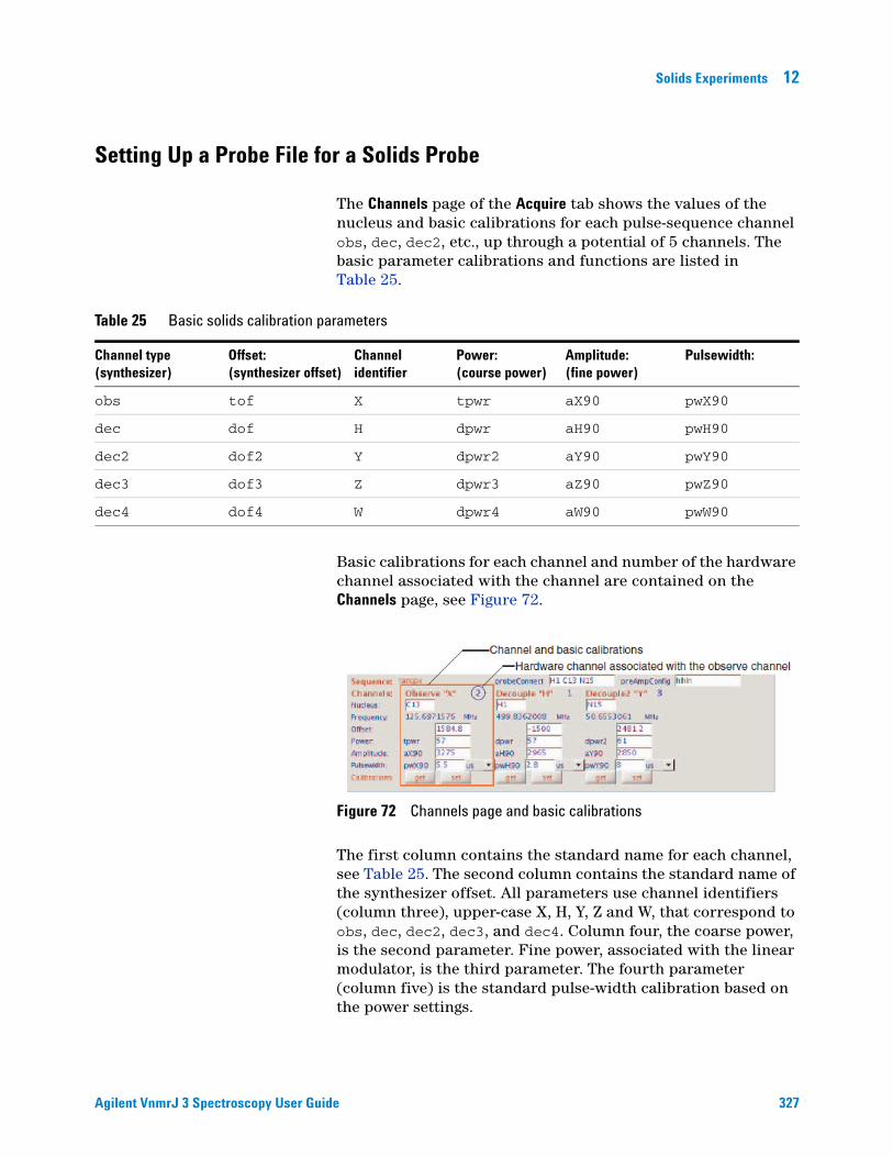
Solids Experiments 12
Setting Up a Probe File for a Solids Probe
Agilent VnmrJ 3 Spectroscopy User Gui
The Channels page of the Acquire tab shows the values of the nucleus and basic calibrations for each pulse-sequence channel obs, dec, dec2, etc., up through a potential of 5 channels. The basic parameter calibrations and functions are listed in Table 25.
Table 25 Basic solids calibration parameters
Channel type (synthesizer)
Offset: (synthesizer offset)
Channel identifier
Power: (course power)
Amplitude: (fine power)
Pulsewidth:
obs tof X tpwr aX90 pwX90
dec dof H dpwr aH90 pwH90
dec2 dof2 Y dpwr2 aY90 pwY90
dec3 dof3 Z dpwr3 aZ90 pwZ90
dec4 dof4 W dpwr4 aW90 pwW90
Basic calibrations for each channel and number of the hardware channel associated with the channel are contained on the Channels page, see Figure 72.
The first column contains the standard name for each channel, see Table 25. The second column contains the standard name of the synthesizer offset. All parameters use channel identifiers (column three), upper-case X, H, Y, Z and W, that correspond to obs, dec, dec2, dec3, and dec4. Column four, the coarse power, is the second parameter. Fine power, associated with the linear modulator, is the third parameter. The fourth parameter (column five) is the standard pulse-width calibration based on the power settings.
Figure 72 Channels page and basic calibrations
de 327

328
12 Solids Experiments
Click the Set button for each channel to save changes to the probe file for the set of basic calibrations for each nucleus to the probe file. The current value of the nucleus is attached to the values in the probe file. If needed, a new nucleus will be added to the probe file. An acknowledgement that the data is saved appears in the Message window.
Click the Get button for each channel to retrieve calibrations from the probe file. An error message appears in the Message Window if calibrations are not present. The current nucleus for the channel is used to choose the calibrations.
Use the Set and Get functions when the observe and decouple channel nuclei are interchanged.
The Settancpx protocol loads basic calibrations from the probe file if the probe file is defined and the nuclei are present in the file. The basic calibrations are the only values stored in the probe file by solids protocols.
Setting the MAS spin rate
The MAS spin rate is controlled through the MAS Spin/Temp page of the Start tab, see Figure 73. VnmrJ 3 sends commands to the MAS Automated Speed Controller by way of the console master controller.
Agilent T3 probes provide the name of the module (for example” 3.2 MM PENCIL”) to the MAS automated speed controller so that the appropriate values are set for start-up and regulation. The module name is also sent to VnmrJ 3 and it is displayed on the MAS Spin/Temp page as Probe ID. VnmrJ 3 uses the module name with underscores between words to automatically set the probe parameter.
Figure 73 Solids spin/temp page with: spintype ='mas'
Agilent VnmrJ 3 Spectroscopy User Guide

Solids Experiments 12
Loading the probe file
Agilent VnmrJ 3 Spectroscopy User Gui
Do one of the following:
• Select and load the probe file corresponding to the probe in use as follows:
a Click Probe on the hardware toolbar to open the Probe pop-up window.
b Select a probe from probes shown in the drop down menu.
c Click Close to load the probe and exit the Probe pop-up window.
• Create the probe file for the probe in use if one does not exist.
a Click Probe on the hardware toolbar to open the Probe pop-up window.
b Select the Edit box.
c Enter a name for the probe.
d Click the Make new probe button.
e Click the Edit Probe button to open the Probe Edit pop-up.
f Click the Probe tab.
g Enter the following information into the probe file:
Press Return after typing each entry into the specified field.
The probe name and these entries are required to display the MAS Spin/Temp page:
a Click OK to save and close the pop-up.
b Select any probe from the probes shown in the drop-down menu.
c Select the name of the solids probe from the drop-down menu. The probe name must be explicitly selected after the probe file has been created.
d Click Close to load the probe file and exit the pop-up window.
Probe file field Value Parameter set
Probespintype mas spintype
Probespinmax Maximum rotor speed in Hz spinmax
de 329

12 Solids Experiments
Starting the rotor
330
1 Set the MAS automated speed controller to AUTO mode.
2 Verify that the correct module name is shown on the MAS Spin/Temp page.
Load (or reload) the correct probe file for the installed probe if the module name is not correct.
3 Select Thin or Std to select the correct Max Speed.
4 Set the Target(Hz) for spinning.
5 Press Start on the MAS Spin/Temp page.
6 Wait for the speed to regulate.
The LOCKED light on the controller is on when spinning is in regulation. The current speed is displayed on the MAS Spin/Temp page and on the controller.
Changing the rotor speed
1 Enter a new Target(Hz) value.
2 Press Return.
3 Wait for the speed to regulate.
Stopping the rotor
Press Stop to stop the rotor.
Setting the bearing pressure
The bearing pressure is set automatically based on the value of Bearing: Max(psi) as roughly a linear function of the Target(Hz) spin rate.
Make a fine adjustment for the bearing as follows:
1 Set Bearing: Span = 0
2 Set the Bearing: Adjust(psi) to the change in pressure, positive or negative.
3 Reset Span = 100 to lock the new bearing pressure in place.
The new bearing pressure can be read from the display on the MAS Automated Speed Controller.
Agilent VnmrJ 3 Spectroscopy User Guide

Solids Experiments 12
Starting the rotor manually
Agilent VnmrJ 3 Spectroscopy User Gui
Start a rotor manually and then put it in regulation as follows:
1 Set the Target(Hz) on the MAS Spin/Temp page.
2 Set the knobs for the drive and bearing pressure valves on the controller counter clockwise.
3 Press the Auto/Manual button on the controller to put it in the manual mode.
4 Obtain stable spinning near the desired speed using the knobs.
5 Press the Auto/Manual button again to put the rotor in regulation.
6 Reset the pressure valves counter-clockwise.
7 Stop the rotor as follows:
Press Stop button on the MAS Spin/Temp page.
It is not possible to return to manual mode while the rotor is spinning.
The Start and Stop buttons on the MAS Automated Speed Controller have the same function as the Start and Stop buttons on the MAS Spin/Temp page.
de 331

12 Solids Experiments
Setting the Temperature
332
The temperature of the rotor is controlled through the VT stack, which sits in the upper bore of the magnet and must be installed before starting solids VT operations. The VT stack replaces the liquids upper barrel and attaches to the top of the probe for wide-bore magnets. The VT stack sits inside the liquids upper barrel in narrow-bore magnets. A heater and thermocouple are present at the exit of the VT stack to provide temperature-controlled gas to the module. Both bearing and drive gas for MAS spinning are maintained at ambient temperature and are separate from the gas used for VT operation. Low temperature cold gas is supplied to the VT stack using a gas cooler, such a cold trap in a liquid nitrogen Dewar or an FTS unit.
Starting temperature regulation
A solids/liquids NMR system pneumatics router has separate gas regulation systems for solids and liquids and a common regulator valve for the VT-gas pressure. Solids gas flow is controlled with a manual valve below the flow meter. A typical flow rate is 40 lpm.
Start temperature regulation as follows:
1 Load the Solids Probe file if it is not already loaded.
The solids meter is selected by loading a solids probe file and entering su.
2 Click the Start tab.
3 Select the Spin/Temp page.
Solids gas flow is set from the solids Spin/Temp page, see Figure 73 on page 328. A set of LEDs are lit on the selected pneumatic router meter.
4 Set the value of the parameter vtc from the command line to a value above the highest expected temperature that requires cooling gas.
A typical value for vtc is 5 °C to 10 °C below the ambient room temperature or the temperature of the VT supply gas.
The choice of gas cooling or the bypass is determined by the parameter vtc, the variable temperature cutoff. A set temperature below vtc chooses gas cooling and a set temperature above vtc chooses the bypass. Choose a value of vtc in the dataset that corresponds to the desired operation.
Agilent VnmrJ 3 Spectroscopy User Guide

Solids Experiments 12
Agilent VnmrJ 3 Spectroscopy User Gui
The standard protocol Settancpx automatically resets vtc = -30. To change the default value of vtc, save a copy the parameter set, Settancpx.par, with the new value of vtc in ~/vnmrsys/parlib. The new parameter set will be loaded each time the protocol Settancpx is loaded by the current user. The change does not affect any of the other users. Make the change available to all users by logging in as the system administrator, vnmr1, and saving Settancpx.par with the new value of vtc in /vnmr/parlib.
The system administrator can edit the file /vnmr/parlib/Settancpx/procpar and change the entry for vtc: vtc 1 1 250 -100 0.1 2 1 2 1 64 1 -30 using vi or any ASCII text editor supplied with the operating system to reflect the new cut-off temperature by changing the value of entry -30 at the end of the vtc line to a new value such as 15. The new entry reads: vtc 1 1 250 -100 0.1 2 1 2 1 64 1 15 The entries for vtc of primary interest are: vtc 1 1 [upper temperature limit] [lower temperature limit] [precision] 2 1 2 1 64 1 [bypass cutoff]
5 Enter su on the command line.
Press the Pneumatics Reset button once or twice if the set up (su) does not proceed.
Liquids flow may persist after selection of solids. Do the following if this happens:
a Load a liquids probe file.
b Press the VT Air Off button on the Spin/Temp panel.
c Reload the solids probe file.
6 Move the Temperature slider control left or right on the Spin/Temp page until the required temperature (°C) is displayed in the field to the left of the slider or enter the temperature regulation value, in °C, in the field to the left of the slider on the Spin/Temp page and press Return.
7 Press the Regulate Temp button.
Press the Reset Pneumatics Router and/or Reset VT Controller buttons before proceeding if the temperature regulation does not set up.
de 333
334
12 Solids Experiments
8 Select the check box for Control Temperature from This Panel Only.
9 Select the error reporting radio button.
The radio button choices below Control Temperature from This Panel Only are:
• Abort after temperature error
• Warn after temperature error
• Ignore temperature error
The parameter temp is a passive indicator of the temperature set in the panel when the Control Temperature from This Panel Only check box is selected. The current value of the parameter temp is used to set the temperature at su or at the start of acquisition if the Control Temperature from This Panel Only is not checked.
Stopping temperature regulation
1 Press the Temp Off button.
2 Reselect a liquids probe and press the VT Air Off button on the Spin/Temp panel.
3 Turn Off the solids gas-flow valve when selecting liquids.
Recovering from a VT fault
The solids VT stack is equipped with a high temperature bypass that bypasses the installed gas cooler that supplies ambient temperature gas to the stack. Narrow bore VT stacks have a gas-flow sensor, a probe-stack integrity sensor, and a bore-temperature sensor that may fault under a variety of error conditions. The temperature controller is disabled and the gas flow is switched to bypass if a fault condition is detected. A small amount of purge gas is vented through the gas cooler to keep it from freezing up.
1 Correct the problem causing the fault condition.
2 Press the Reset Pneumatics Router and Reset VT Controller buttons.
3 Reset the temperature to resume operation.
Agilent VnmrJ 3 Spectroscopy User Guide

Solids Experiments 12
Setting up Single-Pulse Experiments
Agilent VnmrJ 3 Spectroscopy User Gui
Single-pulse excitation is run using the Onepul protocol. The protocol uses the calibrated 90-degree pulse pwX90 from the Channels page of the Acquire tab and provides acquisition with a standard Decoupling parameter group; see “Setting Up Decoupling” on page 338. Decoupling parameters are located on the Pulse Sequence page.
de 335

12 Solids Experiments
Setting up Cross Polarization
336
Cross polarization is run using the Tancpx protocol. The protocol uses the cpHX parameter group for constant, linear, or tangent-ramped cross polarization. The cpHX parameter group is located on the Pulse Sequence page of the Acquire tab and it used in any pulse sequence where cross polarization is needed, see Figure 74.
Calibrate the probe, see “Calibration of 13C-1H CPMAS Probes” on page 353.
Tancpx provides excitation with the basic calibrated 90-degree pulse pwH90 from the Channels page and acquisition with standard Decoupling parameter group located on the Pulse Sequence page, see “Setting Up Decoupling” on page 338.
The cpHX parameter group and upper-case channel identifiers specify the channels involved in cross polarization. The first character is the channel from which the starting polarization is derived and the second is the channel that is polarized. The cpHX parameter group used with Tancpx indicates cross polarization from the dec channel to the obs channel.
The Pulse Sequence page of the Acquire tab for Tancpx, see Figure 74, contains two parameter groups: cpHX for cross polarization and Decoupling for proton decoupling. These parameter groups are used in all sequences that contain cross polarization and proton decoupling functions.
Figure 74 Tancpx pulse sequence page of the acquire tab
Agilent VnmrJ 3 Spectroscopy User Guide

Solids Experiments 12
Menu or Parameter Description
Shape menu Values are: const, linear, or tan.Pulse shape used on one of the two channels for the cpHX parameter group.
Channel menu Values are: from — channel used to apply the shape to the decoupler channel. to — channel used to apply the shape to the observe channel.
aHhx parameter The median amplitude of the decoupler channel and aXhx is the median amplitude of the observe channel.
dHX parameter The +/- amplitude excursion of a linear or tangent ramp about the median value and has no effect on constant CP.
bHX parameter Curvature factor for tangent ramps only.bHX must be greater than 0 (zero). bHX > 10000.0 applies a linear ramp. bHX < 1.0 applies a tangent ramp that is nearly constant with extreme excursions at the beginning and end. Values in between provide tangents of various curvatures.
tHX parameter Contact time.
ofHX parameter Frequency offset applied to the shaped channel as designated by the Channel menu choice.
Agilent VnmrJ 3 Spectroscopy User Gui
The CP parameter group generates it is offset with a phase ramp and the offset adds or subtracts from the value of the synthesizer offset (tof or dof) for the channel.de 337

12 Solids Experiments
Setting Up Decoupling
338
Decoupling during acquisition is carried out in nearly all pulse sequences with the Decoupling parameter group on the Pulse Sequence page of the Acquire tab, see Figure 80 on page 356. Select from the choices: TPPM, SPINAL64, CW decoupling, or decoupler off.
Parameter or Group Description
Decoupling parameter
Menu choices TPPM or SPINAL determine which of the Htppm or Hspinal parameter groups is displayed.
TPPM aHtppm Decoupling amplitude.
pwHtppm Width in microseconds of each of the two pulses (usually just less than a 180-degree pulse).
phHtppm The +/- phase of each of the two pulses. The sign of the phase is that of the first pulse.
SPINAL aHspinal Decoupling amplitude
pwHspinal Width in microseconds of each of the two pulses.(usually just less than a 180-degree pulse).
phHspinal The +/- phase of each of the two pulses of the base cycle.The sign of the phase is that of the first pulse.
SPINAL Applies +/- pulse pairs with a phase of +/-1.0, +/-1.5 and +/-2.0 times phHspinal in a 64-member supercycle.
CW decoupling On with either the TPPM or the SPINAL parameter groups when phHtppm or phHspinal is 0.0.
Off either the TPPM or the SPINAL parameter groups when aHtppm or aHspinal is 0.0.
The decoupling module explicitly associates a decoff() command with an amplitude of 0.0 to gate the decoupler fully off. The typical application with an amplitude of 0.0 only sets the linear modulator to full attenuation.
Agilent VnmrJ 3 Spectroscopy User Guide

Solids Experiments 12
Acquisition Parameters and Other Pages
Agilent VnmrJ 3 Spectroscopy User Gui
The Acquisition page of the Acquire tab provides a customized display of the standard 1D Acquisition parameters and the Receiver gain, see Figure 75.
Figure 75 Acquisition parameters - solids
Field Parameter Description and settings
Spectral Width sw Spectral width, menu select units: Hz, kHz, MHz, or ppm
Acquisition Time at Data acquisition time, menu selections: sec, ms, or µs.
Complex Points np Total number of points collected during the acquisition time.
Recycle Delay d1 First delay in the sequence, menu selections: sec, ms, or µs.
Total Scans nt Total number of transients collected.
Block Size bs Enter number of scans for block size and place a check in the check box to enable.Remove the check from the box to set bs='n', not used, and the block to Total Scans, nt.
Steady State ss Number of dummy scans run before starting data acquisition.
Receiver Gain gain Gain of the receiver. Set the value from 0 to 30 in the field. Select the check box to turn off the autogain function. Do not use autogain with solids.
MAS Rate srate Rotor spin rate, menu select units: Hz, kHz, MHz, or ppm.srate, identifies the spin rate for automatic calculation of synchronized delays in some sequences. The srate parameter is not the same as the setpoint for the MAS Automated Speed Controller on the Spin/Temp page and must be set manually to a value equal to the spin rate.
A check box next to srate sets the parameter hsrotor. Checking this sets the value of srate automatically from the measured spin rate at run time and cannot be used to track the spinning rate while the sequence is running.
Temperature temp Temperature regulation point, select C (centigrade) or K (Kelvin)
Other 2D parameters that are specific to a sequence. The fields are grayed out if the field is not defined. Use par2d if the 2D parameters are required.
de 339

12 Solids Experiments
Default and more pages
340
The Defaults page of the Acquire tab is empty. The More page is used in some sequences to provide space for additional parameter groups that do not fit on the Pulse Sequence page. Content of these pages is specific to the pulse sequence.
Other pages and tabs
The Acquisition, Channels, and Receiver pages that are set up when the Settancpx protocol is loaded have content that is specific to solids sequences. The Future Actions page, Start tab, and Process tab are common to all liquids and solids protocols.
Agilent VnmrJ 3 Spectroscopy User Guide

Solids Experiments 12
Receiver Parameters for Solids
Agilent VnmrJ 3 Spectroscopy User Gui
The Receiver page of the Acquire tab contains parameters that affect the receiver gain, the dead time and phase correction, see Figure 76 on page 341. The dead time is the time after the pulse or cross polarization before acquisition of the first data point.
All solids pulse sequences make use of explicit code for acquisition and avoid using rof2 and alfa. The parameter ddrtc controls the digital receiver time correction and is explicitly defined in solids data sets. Solids protocols do not automatically set ddrtc. The user must set it manually as described below.
Figure 76 Receiver page of the acquire tab, solids
Field name Parameter Values / Description
Receiver Gain (gain) gain Values between 0 and 60, default is 30. Gain can be as low as 0 for very strong signals as for proton experiments. A gain greater than 30 is usually of no benefit.
T/R Switch Delay (rd) rd Values range from 2.0 and 4.0 μs for 1H or 13C to many hundreds of microseconds for low-gamma nuclei with acoustic ringing. The application of rd in solids sequences is analogous to that of the rof2 in other sequences. Set rd to avoid probe ring-down in the first few points of the FID. The delay follows the last pulse or the cross polarization and precedes opening the T/R switch.
Minimum Value of rd (rof3) rd rof3,if defined
Controls the time between the opening of the T/R switch and the receiver turn-on. The value of rof3 can be set greater or less than 2.0 μs. The default time is 2.0 μs if rof3 is not defined.
Multi-pulse sequences explicitly set the value of rof3 so that it can be set to less than 2.0 μs. The value associated with rof3 for multi-pulse sequences, such as BR24, is part of the parameter group of the multi-pulse waveform and is labeled with the prefix r3. Always set rof3 = r3 when running multiple-pulse sequences.
de 341

12 Solids Experiments
Sampling Delay Adjust (ad) ad Values between 4.0 and 10 μs.The application of ad in solids sequences is analogous to that of alfa in other sequences. Typically, the T/R switch (if used) is opened at the beginning of the delay and the receiver is turned on 2.0 μs later. In this case, ad cannot be less than 2.0 μs. The first point is acquired at the end of the delay.
DDR Time Correction (ddrtc) ddrtc Controls automatic back-prediction of the FID in the digital receiver. The first-order phase correction lp will be approximately 0.0 if ddrtc = rd + ad. Fine tune ddrtc to obtain lp = 0.0. The parameter ddrtc corrects the phase for all spectral widths of 1.25 MHz and less.
A correct setting of ddrtc is very effective for automatic phasing, but it does not necessarily produce a flat baseline. One can expect a flat baseline if the value of ddrtc < 1/(2.0*sw) (a usual situation for CPMAS but not for larger spectral widths) and if the true first point of the FID is not distorted.
Field name Parameter Values / Description
342
First-point distortion of the baseline resulting from time correction has characteristic hooks at the outer edges. The spectrum appears to sit in a trough or on a pedestal. Ringing in the back-prediction calculation by bad first points in the FID is the typical cause. The ringing may extend well beyond the first points so this problem cannot be corrected with linear prediction.
Fix the first point distortion by increasing rd until the first point is good. Estimate the first point distortion and set rd by observing the FID with sw = 5.0e6. Choose the new value of rd and then obtain the data with the original spectral width.
Mitigate the effect of a first-point distortion by decreasing the slope of the digital-filter cut-off using the parameter ddrcr as follows:
1 Create the parameter ddrcr (if it does not already exist) by entering the following on the command line: create('ddrcr')
2 Set ddrcr to a value in the range of 5 to 10. The default value (if the parameter does not exist) is 75 and produces steep filters. A lower number decreases the slope of the filters and mitigates the ringing created by bad first points. Linear prediction can readily correct the baseline with a value of ddrtc>1/(2.0*sw) and a good first point.
The prepulse delay, rof1, used in liquids sequences to unblank the transmitter and to preset the phase of pulses, is displayed, but it is not generally used in solids sequences. Solids sequences explicitly preset the phase of pulses at the beginning of the previous delay and the transmitters are continuously unblanked making the pre-pulse delay unnecessary. A pre-pulse delay for multi-pulse sequences, such as BR24, is part of the parameter group of the multi-pulse waveform and is prefixed r1.
Agilent VnmrJ 3 Spectroscopy User Guide

Solids Experiments 12
Tuning a Solids Probe
Agilent VnmrJ 3 Spectroscopy User Gui
Solids experiments require frequent probe tuning, usually for each new rotor. Agilent NMR Systems provide in-line 30-db directional couplers to tap off the reflected power of each channel. A set of reversible 50-db directional couplers are available as an option for solids systems. Probe tuning is carried out with the standard Tune Sweep function of the Probe pop-up window or with the Tunerp protocol associated with the group of solids sequences.
Low power or in-line tuning using tune sweep
Tune the probe using the in-line tune (or low power) method as follows:
1 Install the 30-db couplers correctly with the arrow pointing towards the Front End. Be sure that the arrows on the reversible 50-db couplers point towards the Front End, not the Probe.
2 Click the Probe button.
3 Click the Tune Sweep button in the probe pop-up window.
The Probe tune page replaces the pages in all of the tabs, see Figure 77.
4 The Tune RF channel menu displays the hardware channel to be tuned. The default nuclei selections are: 1H for channel 1, 13C for channel 2, and channels 3 and 4 undefined. The nuclei and frequencies that appear on the Probe tune page are unrelated to those in the Workspace.
5 Select the Channel to be tuned.
6 Select Center Frequency by entering the nucleus from the menu or enter the frequency in the field next to Freq.
7 Choose a value (between 1MHz and 10 MHz) in the field next to Span.
Figure 77 Tune panel - solids
de 343

344
12 Solids Experiments
8 Click the Start Probe Tune button.
9 Press Autoscale to obtain a useful display.
10 Increase the power from 0 to 10 db if the signal-to-noise of the pattern is low.
The tune pulse sequence does not accept powers above 10 db to protect the probe.
11 Decrease the gain if the pattern clips.
12 Adjust the Vertical scale and the Vertical position of the pattern with the buttons or with the center mouse button.
13 Adjust the Span to the region of the tuning dip and adjust the vertical scale as needed.
The large sinusoidal changes of the tuning baseline are expected for tuning in-line with a directional coupler. These sinusoidal changes are the result of standing waves on the input cables between the preamplifier and the probe caused by the effectively infinite impedance of the probe outside the region of the tuning dip.
Some systems have channels with high-power low-band preamplifiers. These preamplifiers use passive diodes that cut off the input tune signal if it falls to too low a value and in some frequency ranges the pattern has no amplitude. Increase the gain to 10 on the channel if this occurs. The gain may still be too low to observe a tune dip. Bypass the preamplifier by connecting the cable on the XMTR port of the preamp to the cable attached to the PROBE port if increasing the gain is not enough. The amplitude of the pattern is affected by the presence of filters in-line with the input cables.
14 Tune the probe (see the probe manual to determine the correct knobs on the probe).
Figure 78 Tuning pattern, solids
Agilent VnmrJ 3 Spectroscopy User Guide

Solids Experiments 12
Agilent VnmrJ 3 Spectroscopy User Gui
The tuning pattern, see Figure 78, is a dip of the reflected power near zero when the probe is tuned. The width of the dip approximates the bandwidth of the probe.
15 Press Stop Probe Tuning to halt tuning.
16 Press Quit to return to the data in the Workspace.
High-power tuning
See “High Power Pulse Tuning (Tunerp)” on page 378 for tuning with pulses using the Protocol Tunerp and the reversible 50-db directional couplers.
de 345

12 Solids Experiments
Shimming and Referencing for Solids
Shimming
346
The field homogeneity for a MAS probe is usually optimized with a sample of adamatane. Follow the procedure in “Shimming with adamantane” on page 361.
Referencing for solids
Referencing for Solids is complicated by the fact that a solids probe has no lock channel and there is no lock solvent. As a result, the lock frequency is not necessarily on resonance. VnmrJ 3 automatic referencing uses the setref command, the file /vnmr/nuctables/nuctabref, and is dependant upon the lock being on resonance.
Set the lock frequency on resonance as follows:
1 Recall a referenced 13C spectrum of adamantane.
2 Click the Start tab.
3 Select the Lock page.
4 Click the Lock OFF radio button.
5 Enter 0.0 in the field next to the Z0 button if the value in the field it is no 0.0.
6 Insert a rotor containing adamatane and install the probe.
7 Shim using the adamantane signal.
8 Acquire a spectrum and reference the higher ppm line to 38.3 ppm.
9 Put a cursor on the line and type calclockfreq(38.3p).
10 Note the value of lockfreq in the message window.
11 The value of lockfreq is set to at least the fifth place after the decimal point.
12 Acquire a spectrum and reference the higher ppm line to 38.3 ppm (see Figure 79).
Agilent VnmrJ 3 Spectroscopy User Guide

Solids Experiments 12
Agilent VnmrJ 3 Spectroscopy User Gui
13 Reacquire the spectrum and type setref.
14 Set the correct value for lockfreq into the configuration parameters in the vnmr1 user. The value of lockfreq is lost when logging out of the user if it is not saved.
The correct value of the lock frequency depends upon the choice of the lock solvent. Choose a constant value of solvent (for example CHCL3) to be used for solids data. Referencing remains correct until the magnet has drifted outside the solids lineshape, usually after a couple of days.
The reference display of VnmrJ 3 does not correct itself if the spectral width sw or the offset tof is reset. Re-establish the reference based on the lock with setref after changing these parameters.
Figure 79 Adamantane reference spectrum
de 347

12 Solids Experiments
Using probeConnect with Solids
348
The transmitter associated with each pulse-sequence channel is displayed to the right of the channel name in the Channels page of the Acquire tab, see “Channels page and basic calibrations” on page 327.
A two-channel Agilent NMR System is always configured with channel 1 as the high-band transmitter and channel 2 as the low-band transmitter if the sfrq > 0.85 times the proton frequency. Otherwise, the transmitters are reversed. The system always sets the correct band based on the nucleus.
Agilent NMR System with more than two channels and a pulse sequence that uses more than two channels must use the parameter probeConnect. The probeConnect parameter does not need definition if only channels 1 and 2 are used. Channels 3 and 4 can be configured as either high-band or low-band. Entry boxes for probeConnect and preAmpConfig are on the top line of the Channels page (Figure 72 on page 327). The value of probeConnect is initially undefined, as indicated by dashes in the box.
Creating the probeConnect parameter
1 Verify the existence of the probeConnect parameter as follows:
a Enter probeConnect on the command line.
b Continue with step 2 if the message in the message box is:
c Variable “probeConnect” doesn’t exist
d Skip to Step 3 if there is no message reporting that the variable does not exist.
2 Enter the following on the command line:
create('probeConnect','string','global')
3 Enter the nucleus associated with each channel in order, channel 1, channel 2, etc. and separate each entry with a space.
The entries in the probeConnect field identify the nuclei that are associated with each hardware channel. Change the entries in the probeConnect field to correspond to a new probe-tuning configuration.
Agilent VnmrJ 3 Spectroscopy User Guide
Solids Experiments 12
Using probeConnect during the decoupler calibration process
Agilent VnmrJ 3 Spectroscopy User Gui
1 Set the decoupler nuclei one by one in the Nucleus field of the Observe ''X'' section in the Channels page of the Acquire tab and determine the basic calibrations using the Onepul experiment.
2 Click the Set button to enter the calibration into the probe file.
3 Return each nucleus to its proper decoupler channel when the calibrations are complete.
4 Click the Get button to reload the decoupler calibrations.
de 349

12 Solids Experiments
Using preAmpConfig with Solids
350
The value of preAmpConfig indicates the type of preamplifier- high-band or low-band, that is associated with each hardware channel. The default is preAmpConfig = 'hlnnn' where 'h' means high-band, 'l' means low-band and 'n' means no preamplifier. The characters of preAmpConfig are the hardware channels. The third to fifth characters of preAmpConfig should be changed to their correct values if preamplifiers are present on channels 3 to 5.
Agilent VnmrJ 3 Spectroscopy User Guide

Solids Experiments 12
Using hipwrampenable for Solids
Agilent VnmrJ 3 Spectroscopy User Gui
An Agilent NMR System with high-power (kilowatt) amplifiers contains relay boards to select high power for solids or low power for liquids. The default selection for the relay board is low power by default unless the parameter hipwrampenable is created. High power is defined as the specified amplifier output (usually a kilowatt, but a bit less for high-band amps at 600 MHz and above). Low power is defined as 50 Watts for high band and 300 Watts for low band. High power NMR Systems use the high band driver to provide the 50 Watts and they attenuate input of the low band kilowatt amp to provide the 300 Watts.
1 Verify the existence of the hipwrampenable parameter as follows:
a Enter hipwrampenable on the command line.
b Continue with step 2 if the message in the message box is: Variable ''hipwrampenable'' doesn’t exist
c Skip Step 2 if there is no message reporting that the variable does not exist.
2 Enter the following on the command line:
create('hipwrampenable','string','global')
The parameter hipwrampenable is a global parameter and applies to all data sets in a user and can only be accessed from the command line.
'y' enables high power or the RF channel.
'n' enables low power and disables high power for the RF channel.
A character is required for each hardware channel up to the total number of channels numrfch. The value of numrfch is 3 for system with three RF channels and high power on channel 1 and low power on the remaining channels is specified as:
hipwrampenable='ynn'
de 351

12 Solids Experiments
Using Amplifier Blanking and Unblanking for Solids
352
All solids sequences are written to maintain amplifiers on all channels as unblanked throughout the pulse sequence, except during acquisition. This convention is different from the convention used by the Agilent NMR System for liquids sequences (and older solids sequences). Continuous unblanking maintains each amplifier temperature on or hot to provide greater amplifier stability.
Solids sequences execute the unblank command on the obs channel before the recycle delay d1 and the sequence ends with an unblank after the acquisition. The same pattern of blanking and unblanking is repeated for the decouplers. Liquids sequences (and older solids sequences) execute the unblank on the obs channel before the first pulse or turn it on and off before and after the pulses. The decouplers have no blank and unblank commands and they use the decoupler amplifiers in continuous mode.
Solids sequences provide the option to blank decouplers during acquisition. The decoupler amplifiers must be set to pulsed mode by setting the decoupler channel ampmode to 'p' instead of 'd'. All solids data sets contain the ampmode parameter for this purpose. Blanking dec2 or dec3 during acquisition when using a 3-channel HXY probe delivers better performance.
Very high stability also requires that amplifiers remain on between experiments. Consult the VnmrJ 3 Installation and Administration user guide to set solids mode. The solids mode has no effect on the state of the amplifiers when the sequence is running.
Agilent VnmrJ 3 Spectroscopy User Guide

Solids Experiments 12
Calibration of 13C-1H CPMAS Probes
Agilent VnmrJ 3 Spectroscopy User Gui
Use the following calibration procedure for 13C-1H CPMAS probes and VnmrJ 3 30C released sequences. Use the signal to noise test to verify the calibrations and as a routine system performance check.
These procedures use the Onepul and Tancpx protocols and related sequences.
Sample preparation
Pack 2 rotors as follows:
• 50% (by weight or volume) adamantane and potassium bromide (Adamatane/KBr).
• Full rotor of hexamethylbenzene (HMB).
Setting up the workspace for calibration
Do one of the following:
• A calibration data set exists:
a Select the protocol Settancpx from the Basic ID Experiments directory of the Experiment Panel pull-down menu.
b Set tn = 'C13' and dn = 'H1'. The Settancpx protocol loads any existing calibrations from the probe file. Do not use the calibrations that are shown unless they are known to be correct.
• A calibration data set does not exit:
Load a previous 13C-1H spectrum or parameter set for the particular solids probe configuration to be used, if one is available.
Tuning the probe
1 Verify that all cables are correctly connected to the probe.
2 Place the adamantane/KBr rotor in the module.
3 Raise the probe into the magnet.
4 Spin the sample at 5.0 kHz.
5 Press the Probe button on the lower bar.
6 Click Tune Sweep in Probe pop-up window.
de 353

354
12 Solids Experiments
Tune Sweep starts the mtune program and loads the Tune Panels.
7 Set Channel 1 to H1 using the drop-down menu.
8 Click Start Probe Tune.
9 Follow the procedures in “Tuning a Solids Probe” on page 343.
10 Set Channel 2 to C13 using the drop-down menu.
11 Click Start Probe Tune.
12 Follow the procedures in “Tuning a Solids Probe” on page 343.
13 Repeat the tuning of channels 1 and 2 iteratively until the optimal tuning is obtained.
14 Press Quit Probe Tune to return the workspace.
Calibrating the 1H pw90
1 Load the Onepul protocol from the Experiment Selector or select it from the Experiment menu on the main menu bar.
2 Click the Acquire tab.
3 Click the Acquisition page.
4 Type the following values in the associated fields:
5 Click the Channels page.
6 Enter H1 in the Nucleus field for the Observe ''X'' channel.
7 Enter C13 in the Nucleus field for the Decouple ''H'' channel.
8 Remove any entries in the Nucleus fields for the Decouple2 ''Y'' and Decouple3 ''Z’’ channels if these fields are present.
9 Set the starting calibrations if necessary.
Field Value
Spectral Width 1.0e5 Hz
Acquisition Time 0.003 s
Recycle Time 5.0 s
Gain 0.0
Scans 1
Agilent VnmrJ 3 Spectroscopy User Guide

Solids Experiments 12
CAUTION Excessive power can damage to the probe and amplifiers. Verify the type and placement of installed attenuators on the system before setting tpwr>54. Some system managers choose to use attenuators on the input of the transmitter to allow a tpwr setting higher than 54 with a high power amplifier.
Agilent VnmrJ 3 Spectroscopy User Gui
• Low-power system (100 Watts 1H)
• High-power system (nominally 1000 Watts 1H)
10 Click the Acquire tab.
11 Select the Pulse Sequence page.
12 Select the TPPM decoupling option.
13 Set aHtppm = 0.0 to turn off the decoupler.
14 Set phHtppm = 0.0 to set CW decoupling for future tests.
15 Click the Acquire button to start the experiment
16 Put a cursor on the center peak and type movetof on the command line to move the transmitter on resonance.
17 Array pwX90 from 1.0 to 25.0 µs in steps of 1.0 µs.
18 Click the Acquire button to obtain the array.
The data will look similar to Figure 80.
Field Value
tpwr 63
aX90 2000
pwX90 4.0 µs.
Field Value
tpwr 54
aX90 2000
pwX90 4.0 µs.
de 355

356
12 Solids Experiments
19 Estimate the 90-degree pulse as one-half the 360-degree minus the 180-degree pulse. Ignore the broad line. It is probe 1H background.
20 Adjust the value of aX90 to obtain a 90-degree 1H pulse pwX90 equal to the 1H target pulse width or pulse specification.
21 Reduce tpwr and increase aX90 as required to place aX90 in the range of 3500 to 4095. Lowering tpwr by 6 db increase aX90 by 2 fold.
22 Save the data and record the values.
The value of aX90 serves as the maximum value for aHtppm or aHspinal.
23 Readjust the value of aX90 to obtain a 1H 90-degree 1H pulse pwX90 equal to the 13C pulse specification, see Figure 81.
24 Save the data and record the values.
Use this 1H amplitude for cross polarization as aHhx in the cpHX parameter group.
Figure 80 CPMAS pwX90 1H calibration array
Figure 81 CPMAS pwX90 for 4.0 ìs 1H 90-degree pulse
Agilent VnmrJ 3 Spectroscopy User Guide

Solids Experiments 12
CAUTION Damage to the probe can result if this field strength is exceeded. This field strength is the maximum that should be used in cross-polarization. Calibrate a cross-polarization amplitude lower than the specification as required by the experiment or general operating practice. A 1H pulse width of 4.0 to 5.0 μs works for most experiments and the lower power reduce wear and tear on the probe.
Agilent VnmrJ 3 Spectroscopy User Gui
25 Enter these second 1H basic calibrations on the Channels page of the Acquire tab.
26 Press the Set button for obs and dec on the Channels page to save the 1H calibration and the existing 13C numbers in the probe file.
Calibrating the 13C pw90
Continue in the same workspace using the Onepul protocol and maintain the Adamantane/KBr sample at 5.0 kHz.
1 Click the on the Acquire tab.
2 Select the Acquisition page.
3 Set the following:
4 Click the Channels page.
5 Enter C13 in the Nucleus field for the Observe ''X'' channel.
6 Enter H1 in the Nucleus field for the Decouple ''H'' channel.
7 Press the Get button for Observe and Decouple to retrieve the most recent 1H and 13C calibrations from the probe file under the correct nucleus settings.
8 Set the starting calibrations for 13C if necessary.
Field Value
Spectral Width 5.0e4 Hz
Acquisition Time 0.02 s
Recycle Time 5.0 s
Gain 30
Scans 1
de 357

12 Solids Experiments
CAUTION Excessive power can damage to the probe. Verify the type and placement of installed attenuators on the system before setting tpwr>54. Some system managers choose to use attenuators on the input of the transmitter to allow a tpwr setting higher than 54 with a high power amplifier.
358
• Low-power system (300 Watts 13C)
• High-power system (nominally 1000 Watts 1H)
9 Click the Acquire tab.
10 Select the Pulse Sequence page.
11 Select the TPPM decoupling option.
12 Set aHtppm = aH90 value and use the aH90 from the Channels page.
13 Set phHtppm = 0.0 for CW decoupling.
14 Enter lb = 50 to set the line broadening to 50 Hz.
15 Click the Acquire button.
16 Place the transmitter between the two peaks of Adamantane.
17 Put one cursor on each peak.
18 Enter split movetof on the command line.
19 Reduce the Spectral Width to 5 to 10 kHz (600 MHz and above).
20 Array pwX90 from 1.0 to 25.0 µs in steps of 1.0 µs.
21 Click the Acquire button to acquire the arrayed data.
The result is similar to Figure 82.
Field Value
tpwr 63
aX90 2000
pwX90 4.0 µs.
Field Value
tpwr 54
aX90 2000
safety limit -ON 54
Agilent VnmrJ 3 Spectroscopy User Guide

Solids Experiments 12
Agilent VnmrJ 3 Spectroscopy User Gui
22 Adjust the value of aX90 to obtain a 90-degree 13C pulse pwX90 equal to the 1H values. The values may be either the 13C specification or a lower value as determined for the second 1H calibration.
23 Reduce tpwr and increase aX90 as required, to place aX90 in the range of 3500 to 4095. Lowering tpwr by 6 db increases aX90 by 2 fold.
24 Save the data and record the values.
The value of aX90 is used for cross polarization as aXhx in the cpHX group.
25 Enter the 13C basic calibrations on the Channels page.
26 Press the Set button for Observe and Decouple on the Channels page to save the 13C and 1H calibrations in the probe file.
Figure 82 CPMAS pwX90 for 4.0 ìs 13C 90-degree pulse
Magic-Angle adjust with KBr
Continue in the same workspace using the Onepul protocol and the Adamantane/KBr sample at 5.0 kHz.
1 Click the Acquire tab.
2 Select the Acquisition page.
3 Set the following:
4 Select the Channels page.
Field Value
Spectral Width 1e5 Hz
Acquisition Time 0.02 s
Recycle Delay 0.2 s
Gain 30
Scans 16
de 359

360
12 Solids Experiments
5 Enter Br79 in the Nucleus field for the Observe ''X'' channel and be sure the following transmitter number is 2.
6 Do not readjust probe tuning for 79Br.
7 Click the Pulse Sequence page.
8 Select the TPPM decoupling option.
9 Set aHtppm = 0 to turn off decoupling.
10 Click the Acquire button.
11 Place the cursor on the tall center band.
12 Type movetof command.
13 Click the Acquire button.
The result is similar to Figure 83.
14 Enter the Interactive mode with the Fidscan button on the Shims page of the Start tab.
15 Adjust the magic-angle adjust-knob or screwdriver-adjust on the bottom of the probe to maximize the number of spikes (rotational echoes).
The result is similar to Figure 84A when the rotor angle is adjusted match the magic angle. The rotational echoes have the same T2 as the central line and the magic angle is optimal.
Figure 83 Spectrum of KBr to optimize the Magic Angle
Agilent VnmrJ 3 Spectroscopy User Guide

Solids Experiments 12
Agilent VnmrJ 3 Spectroscopy User Gui
Improperly set rotor angle produces echoes that decay more quickly and the result is similar to Figure 84B.
16 Save the data.
17 Continue with “Shimming with adamantane” .
Figure 84 KBr FID for Magic Angle adjustment
Shimming with adamantane
Continue in the same workspace using the Onepul protocol and the Adamantane/KBr sample at 5.0 kHz.
1 Click the Acquire tab.
2 Select the Acquisition page.
3 Set the following parameters:
4 Select the Channels page.
5 Enter C13 in the Nucleus field for the Observe ''X'' channel.
6 The transmitter will remain set to 2. The 13C calibrations were not changed and should remain from the previous step. Press the Get button for both the Observe ''X'' and Decouple ''H'' channels to retrieve the calibrations or if there is any doubt that the calibrations shown are not correct.
7 Click the Pulse Sequence page.
Field Value
Spectral Width 5e3 Hz
Acquisition Time 0.1 s
Recycle Delay 5 s
Gain 30
Scans 1
de 361

362
12 Solids Experiments
8 Select TPPM decoupling.
9 Set aHtppm = aH90/3.0, use the value of aH90 determined in step 23 of “Calibrating the 1H pw90” on page 354.
CAUTION Adamantane shimming will ultimately use an Acquisition Time = 0.4 s. Probe damage will result if the amplitude of decoupling with acquisition time exceeds aH90/2.0. Do not exceed the probe specification for the maximum time the decoupler can be on at an amplitude greater than aH90/2.0. That number is usually 50 ms.
10 Set phHtppm = 0 for CW decoupling.
11 Enter 0.0 in the field next to line broadening under Weighting Parameters and clear the check boxes next to any of the other weighting parameters. This sets lb = 0.0 and places a check in the box next to line broadening field.
12 Click the Acquire button to acquire the data.
A spectrum similar to Figure 85B is a typical example of data acquired when the field homogeneity is poor (poorly shimmed field). A well-shimmed field produces a spectrum of Adamantane, see Figure 85A, with a line width between 0.005 and 0.025 ppm (2 to 10 Hz at 400 MHz). The left hand line is referenced at 38.3 ppm.
Figure 85 Adamantane spectra
Agilent VnmrJ 3 Spectroscopy User Guide

Solids Experiments 12
Agilent VnmrJ 3 Spectroscopy User Gui
13 Place the transmitter between the two lines of Adamantane.
a Select 2 cursors and place them on the two lines of Adamantane.
b Enter split movetof on the command line.
c Click the Acquisition page.
14 Set the spectra width as follows:
15 Click the Acquire button to acquire the data.
16 Click the Channels page.
17 Set an array of the decoupler offset dof from -10000 Hz to 10000 Hz in steps of 1000 Hz.
18 Click the Acquire button to acquire the data.
Figure 86 shows the decoupler offset dependence of a shimmed Adamantane sample. The decoupler must be on resonance.
19 Enter the value of dof corresponding to the spectrum with the greatest peak height.
20 Click the Acquisition page.
21 Set the following:
22 Click the Acquire button.
23 Use Fid Scan on the Shims page of the Start tab to obtain repeating display of the Adamantane spectrum.
System frequency Spectral width
500 MHz and lower 5 kHz
600 MHz and above 10 kHz
Figure 86 Optimizing decoupler offset for adamantane
Field Value
Recycle Delay 5.0 s
Scans 4.
de 363

364
12 Solids Experiments
24 Optimize the shims to obtain a minimum line width.
Typical shims are X1, Y1, Z1, and Z2.
25 Remove the hump at the base of the line with XY and X2Y2.
26 Record a well-shimmed Adamatane spectrum similar to Figure 85A and save the shims with svs on the command line.
27 Continue with “Matching the Hartmann-Hahn condition” .
Matching the Hartmann-Hahn condition
To set up Tancpx:
1 Change samples.
a Replace the Adamantane/KBR sample with the HMB sample.
b Adjust probe tuning.
c Set spin to 3300 Hz or the value in the probe specification sheet.
2 Load the Tancpx protocol using either of the following:
• Use the Experiment Selector.
a Click the Basic tab of the Experiment Selector.
b Click Tancpx
• Use the Solid-State tab.
a Click Experiments.
b Select Solid-State.
c Select Basic 1D Experiments.
d Click Tancpx.
3 Click the Acquire tab.
4 Click the Acquisition page.
5 Set the following:
6 Click the Channels page.
7 Enter 13C in the Nucleus field for the Observe ''X'' channel.
Field Value
Spectral Width 5.0e4
Acquisition Time 0.02 s
Recycle Delay 5.0 s
Gain 30
Scans 4
Agilent VnmrJ 3 Spectroscopy User Guide

Solids Experiments 12
Agilent VnmrJ 3 Spectroscopy User Gui
8 Enter 1H in the Nucleus field for the Decouple ''H'' channel.
9 Press the Get button for both the Observe ''X'' and Decouple ''H'' channels to retrieve the 13C and basic 1H basic calibrations from the previous steps.
10 Click the Pulse Sequence page.
11 Select tppm form the Decoupling drop-down menu.
12 Select const from the Shape menu in the cpHX: parameter group.
13 Set the following parameters in the fields in the cpHX: parameter group
14 Click the Acquire button.
15 Set the transmitter offset tof to place the tall methyl line in the center of the spectrum.
16 Place a cursor on the line and type movetof on the command line.
To adjust the 13C Match Condition:
1 Array aXhx about +/- 1000 units.
2 Click the Acquire button.
3 Enter the value of aXhx producing the maximum signal in the field next to aXhx: on the Pulse Sequence page.
An example of a 12 step aXhx array is shown in Figure 87.
Field (parameter) Set or type the following value in the field
aHhx calibrated 1H amplitude (aH90 from the Channels page)
aXhx calibrated 13C amplitude (ax90 from the Channels page)
tHX 7000 μs
aHtppm calibrated 1H amplitude (aH90 from the Channels page)
phHtppm 0.0 for CW decoupling
de 365

366
12 Solids Experiments
To make the fine adjustment to pwH90:
1 Select the Channels page.
2 Array pwH90 from 1.0 to 25.0 µs in steps of 1.0 µs.
3 Click the Acquire button.
4 Enter the value of pw90 producing the maximum signal in the field next to pwH90: on the Channels page.
5 Continue to “HMB signal-to-noise ” .
Figure 87 Array of aXhx for 13C Hartmann Hahn match
HMB signal-to-noise
1 Set an array of the number of scans, with 10 repeated values of 4.
2 Click the Acquire button.
10 spectra are acquired with the optimum values from “Matching the Hartmann-Hahn condition” on page 364.
3 Save the data.
4 Set two cursors with delta = 100p for each spectrum and place the right cursor at the right edge of the spectrum.
5 Type dsnmax on the command line to measure the signal-to-noise ration.
6 Record the value.
7 Average 10 values.
Typical array is shown in Figure 88.
Agilent VnmrJ 3 Spectroscopy User Guide

Solids Experiments 12
Agilent VnmrJ 3 Spectroscopy User Gui
8 Continue to “Create a starting data set” .
Figure 88 HMB signal to noise, 10 repetitions
Create a starting data set
1 Load the data from “HMB signal-to-noise ” on page 366.
2 Place the cursor at 100 ppm.
3 Enter movetof.
4 Set the transmitter offset at 100 ppm.
5 Click the Acquire button.
6 Reference the methyl line of the spectrum at 17.3 ppm.
7 Set the cursor on the methyl line.
8 Enter rl(17.3p) on the command line.
9 Click the Acquire button.
10 Set Shape = 'linear' and dHX about 200 in the cpHX parameter group.
11 Optional: Set ramped cross-polarization.
12 Set the receiver parameters correctly and ddrtc = ad + rd.
13 Click the Acquire button.
14 Save the dataset.
A standard HMB spectrum centered at 100 ppm, see Figure 89, obtained with ramped cross-polarization. This spectrum is a starting point for all 13C CPMAS experiments.
de 367

368
12 Solids Experiments
Figure 89 A standard HMB spectrum centered at 100 ppm
Agilent VnmrJ 3 Spectroscopy User Guide

Solids Experiments 12
Basic 1D Experiments
Constant, linear, or tangent cross polarization (CP) (Tancpx)
Agilent VnmrJ 3 Spectroscopy User Gui
Constant, linear, or tangent-ramped cross-polarization (CP) between H and X with a choice of SPINAL64 or TPPM decoupling. Used for calibration of the Hartmann-Hahn Match and calibration of the 90° pulse width pwH90 with X detection.
Protocol Sequence Apptype
Tancpx tancpx.c solidsseq1d
One pulse (Onepul)
Single-pulse preparation with a choice of SPINAL64 or TPPM decoupling. Used for calibration of the 90 pulse width pwX90.
Protocol Sequence Apptype
Onepul onepul.c solidsseq1d
Lee-Golburg CP (Lgcp)
Lee-Goldburg cross polarization (CP) between H and X with a choice of SPINAL or TPPM decoupling. Used for selective CP with suppression of homonuclear dipolar interactions and for setup of Lee-Goldburg HETCOR.Protocol Sequence Apptype
Lgcp lgcp.c solidsseq1d
One-Pulse with TOSS (Onepultoss)
Four pulse TOSS side-band suppression is applied to X after single-pulse excitation, with a choice of SPINAL64 or TPPM decoupling. Used to obtain sideband-free spectra.
Protocol Sequence Apptype
Onepultoss.c Onepultoss.c solidsseq1d
de 369

12 Solids Experiments
pwX90 Measurement with CP (Tancpxflip)
370
Constant, linear, or tangent-ramped cross polarization (CP) between H and X with an X flip-back pulse and a choice of SPINAL64 or TPPM decoupling. Used for calibration of pwX90 with CP and X detection.
Protocol Sequence Apptype
Tancpxflip tancpxflip.c solidsseq1d
CP with FSLG Decoupling (Tancpxfslg)
Constant, linear, or tangent-ramped cross polarization (CP) between H and X followed by FSLG decoupling during acquisition. Used to evaluate FSLG decoupling for use in HETCOR. Tancpxfslg automatically sets up FSLG based upon calibrated values of aH90 and pwH90, using the macro reset_fslg.
Protocol Sequence Apptype
Tancpxfslg tancpxflslg.c solidsseq1d
H T1 with CP (Tancpht1)
An H T1 measurement using inversion recovery followed by X detection with constant, linear or tangent-ramped cross polarization (CP) between H and X with a choice of SPINAL64 or TPPM decoupling. Used for proton T1 measurements with CP.
Protocol Sequence Apptype
Tancpht1 tancpht1.c solidsseq1d
Interrupted Decoupling with CP (Tancpxidref)
Interrupted decoupling for suppression of the signals of protonated X nuclei. Follows constant, linear, or tangent-ramped cross-polarization (CP) between H and X with a choice of SPINAL64 or TPPM decoupling. Provides a refocusing pulse, synchronized with two rotor periods to avoid a large first order phase correction. Used to edit protonated X nuclei from a CPMAS spectrum.
Protocol Sequence Apptype
Tancpxidref tancpxidref.c solidsseq1d
Agilent VnmrJ 3 Spectroscopy User Guide
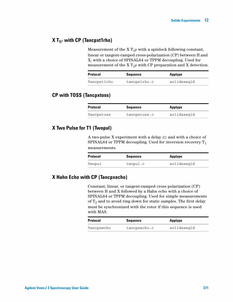
Solids Experiments 12
X T1ρ with CP (Tancpxt1rho)
Agilent VnmrJ 3 Spectroscopy User Gui
Measurement of the X T1ρ with a spinlock following constant, linear or tangent-ramped cross-polarization (CP) between H and X, with a choice of SPINAL64 or TPPM decoupling. Used for measurement of the X T1ρ with CP preparation and X detection.
Protocol Sequence Apptype
Tancpxt1rho tancpx1rho.c solidsseq1d
CP with TOSS (Tancpxtoss)
Protocol Sequence Apptype
Tancpxtoss tancpxtoss.c solidsseq1d
X Two Pulse for T1 (Twopul)
A two-pulse X experiment with a delay d2 and with a choice of SPINAL64 or TPPM decoupling. Used for inversion recovery T1 measurements.
Protocol Sequence Apptype
Twopul twopul.c solidsseq1d
X Hahn Echo with CP (Tancpxecho)
Constant, linear, or tangent-ramped cross polarization (CP) between H and X followed by a Hahn echo with a choice of SPINAL64 or TPPM decoupling. Used for simple measurements of T2 and to avoid ring down for static samples. The first delay must be synchronized with the rotor if this sequence is used with MAS.
Protocol Sequence Apptype
Tancpxecho tancpxecho.c solidsseq1d
de 371
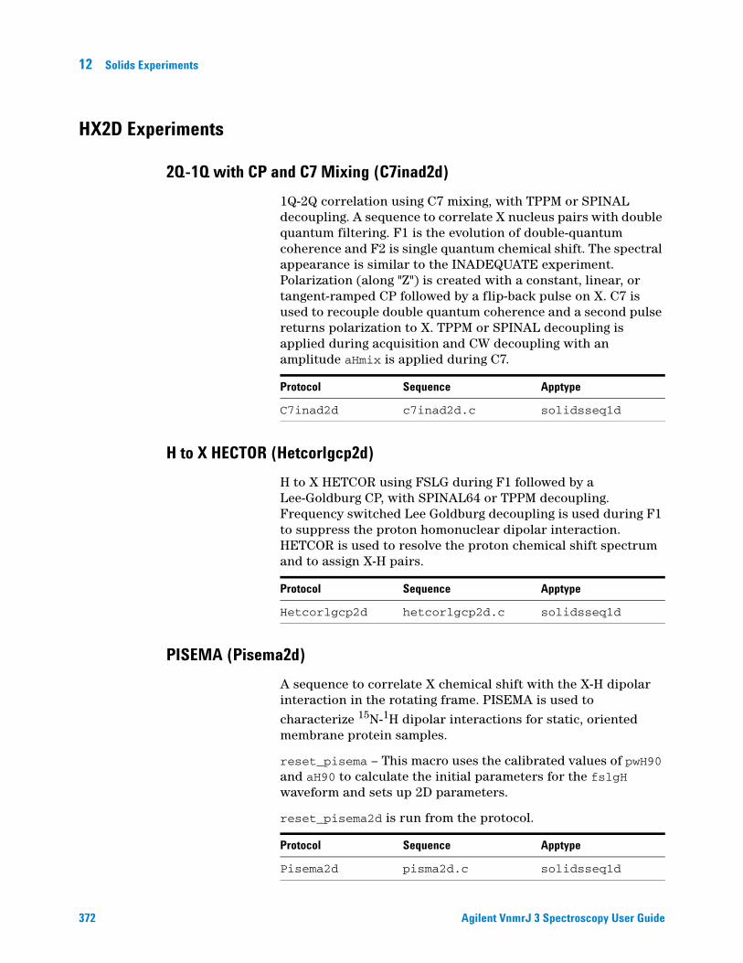
12 Solids Experiments
HX2D Experiments
2Q-1Q with CP and C7 Mixing (C7inad2d)
372
1Q-2Q correlation using C7 mixing, with TPPM or SPINAL decoupling. A sequence to correlate X nucleus pairs with double quantum filtering. F1 is the evolution of double-quantum coherence and F2 is single quantum chemical shift. The spectral appearance is similar to the INADEQUATE experiment. Polarization (along "Z") is created with a constant, linear, or tangent-ramped CP followed by a flip-back pulse on X. C7 is used to recouple double quantum coherence and a second pulse returns polarization to X. TPPM or SPINAL decoupling is applied during acquisition and CW decoupling with an amplitude aHmix is applied during C7.
Protocol Sequence Apptype
C7inad2d c7inad2d.c solidsseq1d
H to X HECTOR (Hetcorlgcp2d)
H to X HETCOR using FSLG during F1 followed by a Lee-Goldburg CP, with SPINAL64 or TPPM decoupling. Frequency switched Lee Goldburg decoupling is used during F1 to suppress the proton homonuclear dipolar interaction. HETCOR is used to resolve the proton chemical shift spectrum and to assign X-H pairs.
Protocol Sequence Apptype
Hetcorlgcp2d hetcorlgcp2d.c solidsseq1d
PISEMA (Pisema2d)
A sequence to correlate X chemical shift with the X-H dipolar interaction in the rotating frame. PISEMA is used to
characterize 15N-1H dipolar interactions for static, oriented membrane protein samples.
reset_pisema – This macro uses the calibrated values of pwH90 and aH90 to calculate the initial parameters for the fslgH waveform and sets up 2D parameters.
reset_pisema2d is run from the protocol.
Protocol Sequence Apptype
Pisema2d pisma2d.c solidsseq1d
Agilent VnmrJ 3 Spectroscopy User Guide

Solids Experiments 12
WISE (Wisentancp2d)
Agilent VnmrJ 3 Spectroscopy User Gui
2D correlation between the X chemical shift and the H wideline spectrum using constant, linear, or tangent-ramped cross-polarization (CP) between H and X with a choice of SPINAL64 or TPPM decoupling. Used for separation of the proton wideline spectra of XH pairs with tHmix = 0. Used for spin diffusion measurements with tHmix > 0.0.
Protocol Sequence Apptype
Wisetancp2d wisetancp2d.c solidsseq1d
de 373

12 Solids Experiments
HXY Experiments
One Pulse REDOR with XY8 on X and Y (Redor1onepul)
374
Rotational Echo Double Resonance (REDOR) with one-pulse preparation, XY8 decoupling with pulses alternating on X and Y, with a choice of SPINAL64 or TPPM decoupling during both acquisition and REDOR evolution. Used to measure XY bond distances for organic materials where one-pulse preparation is preferred.
Protocol Sequence Apptype
Redor1onepul redor1onepul.c solidsseq1d
CP REDOR with XY8 on X and Y (Redor1tancp)
Rotational Echo Double Resonance (REDOR) with constant, linear, or tangent-ramped preparation, XY8 decoupling with pulses alternating on X and Y, with a choice of SPINAL64 or TPPM decoupling during both acquisition and REDOR evolution. Used to measure XY bond distances for organic materials.
Protocol Sequence Apptype
Redor1tancp redor1tancp.c solidsseq1d
One Pulse REDOR with XY8 Y with X Inversion (Redor2onepul)
Rotational Echo Double Resonance (REDOR) with one-pulse preparation, XY8 decoupling with pulses on Y, and a refocusing pulse on X, with a choice of SPINAL64 or TPPM decoupling during both acquisition and REDOR evolution. Used to measure XY bond distances for inorganic and organic materials where one-pulse preparation is preferred.
redor2onepul is the favored REDOR sequence if homonuclear coupling or quadrupole coupling is present for the X nuclei. Rotationally synchronized pi pulses interfere with the refocusing of these interactions into rotational echoes and dephase the magnetization. redor2onepul has only one refocusing pulse on X.
Protocol Sequence Apptype
Redor2onepul redor2onepul.c solidsseq1d
Agilent VnmrJ 3 Spectroscopy User Guide

Solids Experiments 12
CP REDOR with XY8 on Y with X Inversion (Redor2tancp)
Agilent VnmrJ 3 Spectroscopy User Gui
Rotational Echo Double Resonance (REDOR) with constant, linear, or tangent-ramped preparation, XY8 decoupling with pulses on Y, and a refocusing pulse on X, with a choice of SPINAL64 or TPPM decoupling during both acquisition and REDOR evolution. Used to measure X-Y bond distances for inorganic and organic materials.
redor2tancp is the favored REDOR sequence if homonuclear coupling or quadrupole coupling is present for the X nuclei. Rotationally synchronized pi pulses interfere with the refocusing of these interactions into rotational echoes and dephase the magnetization. redor2tancp has only one refocusing pulse on X.
Protocol Sequence Apptype
Redor2tancp redor2tancp.c solidsseq1d
de 375

12 Solids Experiments
Quadrupole Experiments
3Q-1Q MQMAS with Z-filter (Mqmas3qzf2d)
376
3-quantum multiple-quantum MAS with a third Z-filter pulse and a choice of SPINAL64 or TPPM decoupling. Used to obtain a 2D MQMAS spectrum for all spins 3/2 to 9/2.
Protocol Sequence Apptype
Mqmas3qzf2d mqmas3qzf2d.c solidsseq1d
5Q-1Q MQMAS with Z-filter (Mqmas5qzf2d)
5-quantum multiple-quantum MAS with a third Z-filter pulse and a choice of SPINAL64 or TPPM decoupling. Used to obtain a 2D MQMAS spectrum for all spins 5/2 to 9/2.
Protocol Sequence Apptype
Mqmas5qzf2d mqmas5qzf2d.c solidsseq1d
Quadrupole Echo (Ssecho1d)
A two-pulse solid or quadrupole echo with a choice of SPINAL64 or TPPM decoupling. Used primarily for wideline deuterium NMR.
Protocol Sequence Apptype
Ssecho1d ssecho1d.c solidsseq1d
Agilent VnmrJ 3 Spectroscopy User Guide

Solids Experiments 12
Multipulse Experiments
BR24 with Quadrature Detection (Br24q)
Agilent VnmrJ 3 Spectroscopy User Gui
X acquisition with interleaved BR24. Quadrature phase cycle.
Quadrature BR24 multiple-pulse issued for acquisition of high resolution proton NMR. This sequence uses a variable-length preparation pulse and fine-phase array. These are used for the preparation of the magnetization in quadrature perpendicular to the multiple-pulse axis of precession (1,1,1). The four variable length pulses are calculated assuming that pwXprep has a 90-degree flip angle. BR24 has a cycle time of 36 tau with 24 pulses per cycle.
Set phXprep = -45 degrees. Br24q is used with slow spinning (< 2500 Hz).
Protocol Sequence Apptype
Br24q br24q.c solidsseq1d
MREV8 with Quadrature Detection (Mrev8q)
Quadrature MREV8 multiple-pulse sequence is used for acquisition of high resolution proton NMR. The sequence uses a variable-length preparation pulse and fine phase array to prepare the magnetization in quadrature perpendicular to the multiple-pulse axis of precession (sqrt(1/2),0,sqrt(1/2)).
The four variable-length pulses are calculated assuming that pwXprep has a 90-degree flip angle. MREV8 has a cycle time of 12 tau with 8 pulses per cycle. Set phXprep = 0 degrees. Mrev8q is used with slow spinning (< 2500 Hz).
Protocol Sequence Apptype
Mrev8q mrev8q.c solidsseq1d
Semiwindowless WaHuHa (Swwhh4)
Semi-windowless WaHuHa (SWWHH4) multiple-pulse is issued for acquisition of high resolution proton NMR. This sequence uses 90-degree preparation pulses on X and -X offset by -45 degrees to prepare the magnetization perpendicular to the multiple-pulse axis (1,1,1). SWWHH4 has a cycle time of 6 tau with 4 pulses per cycle. Set phXprep = -45 degrees. SWWHH4 is used with medium speed spinning (8.0 to 14.0 kHz).
de 377

378
12 Solids Experiments
Protocol Sequence Apptype
Swwhh4 swwhh4.c solidsseq1d
High Power Pulse Tuning (Tunerp)
A pulse sequence for pulse tuning through the directional couplers in the VNMRJ 3 display. Tunerp is used for high-power pulsed tuning and for characterization of phase transient. It provides a phase detected output of the pulse that can be displayed in phased or absolute value mode. Launch Tunerp with the Fidscan button on the Shims page in Setup tab.
Measure the ratio of forward to reflected power when using Tunerp. The standard directional couplers are wired to measure reflected power only. The arrow on the side of the coupler should point back toward the Front End to measure reflected power. To measure forward power, reverse the coupler so that the arrow points toward the probe.
A second optional bidirectional coupler is available on some systems. With this coupler, reverse the direction of the arrow by turning the knob on the top.
Protocol Sequence Apptype
Tunerp tunerp.c solidsseq1d
Windowed PMLG-N (Wpmlg1d)
Quadrature, windowless PMLG-N (wPMLG) is used for multiple-pulse acquisition. The sequence uses a composite preparation pulse involving a quadrature phase-shifted 90 and a 54.7-degree pulse along Y to prepare the magnetization perpendicular to the multiple-pulse axis of precession (sqrt(2/3), 0 sqrt(1/3)). The recycle time for wPMLG is: tauXwpmlg = 2.0*(4.0*pwX90)*sqrt(2/3) + B where pwX90 is the 90-degree pulse and B is the window time.
Protocol Sequence Apptype
Wpmlg1d wpmlg1d.c solidsseq1d
2D F1 and Windowed PMLG-N (Wpmlg2d)
2D homonuclear correlation with PMLG in F1, a spin diffusion mixing period and quadrature windowed PMLG (wPMLG) for multiple-pulse acquisition in F2. This sequence uses the composite preparation pulse to put the magnetization along -Y perpendicular to
Agilent VnmrJ 3 Spectroscopy User Guide

Solids Experiments 12
Agilent VnmrJ 3 Spectroscopy User Gui
the PMLG axis of precession. After F1 PMLG, a tilt pulse returns precession to the XY plane and puts the Y axis along Z for cosine peaks and the X axis for sine peaks. A delay of tXmix allows mixing by spin diffusion. A quadrature wPMLG sequence similar to wpmlg1d.c then samples the Z axis magnetization in F2. PMLG and wPMLG are used with moderate-speed spinning (8 to 14 kHz).
Protocol Sequence Apptype
Wpmlg2d wpmlg2d.c solidsseq1d
XX Tuneup (Xx)
X pulses with interleaved acquisition. Used for multipulse calibration of pwX90. Usually performed with a liquid sample or a sample of RTV silicon rubber with slow spinning. Xx can also be used to examine sampling windows and set the blank/unblank delays r1Xxx and r2Xxx.
Xx subtracts probe ring-down with a two-scan (0,2) phase cycle of the preparation pulse and the receiver. The xmxX has 0 phase for all scans. The oscillating pattern will not be symmetric about zero due to a constant signal from probe ringing and background for very short values of tau and when probe proton background is present. Use two scans to see the signal without ringing.
Protocol Sequence Apptype
Xx xx.c solidsseq1d
XmX Tuneup (Xmx)
X pulses with interleaved acquisition and alternating phase. Used for multi-pulse calibration to minimize phase transient. Usually performed with a liquid sample or a sample of RTV silicon rubber with slow spinning. Xmx can also be used to examine sampling windows and set the blank/unblank delays r1Xxmx and r2Xxmx.
Xmx subtracts probe ring-down with a two-scan (0,2) phase cycle of the preparation pulse and the receiver. The xmxX sequence has 0 phase for all scans. The oscillating pattern is not symmetric about zero for very short values of tau and when probe proton background is present due to a constant signal from probe ringing and background. Use two scans to see the signal without ringing.
Protocol Sequence Apptype
Xmx xmx.c solidsseq1d
de 379

380
12 Solids Experiments
Agilent VnmrJ 3 Spectroscopy User Guide

Agilent VnmrJ 3 SpectroscopyUser Guide
13Direct Digital Receiver (DDR)
Application of the Direct Digital Receiver 382
Direct Digital (TM) Receiver Operation 385
381Agilent Technologies

13 Direct Digital Receiver (DDR)
Application of the Direct Digital Receiver
382
The Direct Digital Receiver (DDR) uses a single 80 MHz ADC to digitize the NMR signal directly at the intermediate frequency (IF). Data acquired in all NMR application modes liquids, solids, and imaging benefit from flat baselines, excellent dynamic range, and reduction in artifacts associated with quadrature detection.
Quadrature detection for all NMR applications is eliminated with the Direct Digital Receiver. The NMR signal is sampled directly at the 80 MHz rate and routed through a series of digital signal processing (DSP) chips to down-sample (using proprietary algorithms) and digitally filter the data stream to produce the final spectral width.
Figure 90 shows the first increment of a presat-NOESY experiment conducted on a sample of rat urine (in 10% D2O) using a Salt Tolerant Cold Probe and an NMR system at 600 MHz and a spectral width of 6 kHz. The flat baseline (no baseline correction) is free of artifacts arising from quadrature detection and when combined with the flat frequency response of the time-corrected digital Brickwall filters, allows for quantitative performance even in the presence of a complex biological matrix such as urine.
Figure 90 Presat-NOESY rat urine experiment
Agilent VnmrJ 3 Spectroscopy User Guide
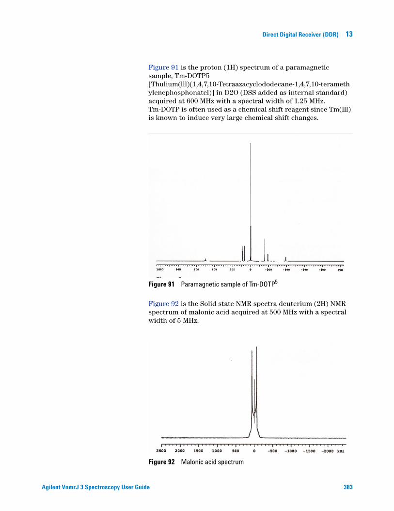
Direct Digital Receiver (DDR) 13
Agilent VnmrJ 3 Spectroscopy User Gui
Figure 91 is the proton (1H) spectrum of a paramagnetic sample, Tm-DOTP5 [Thulium(lll)(1,4,7,10-Tetraazacyclododecane-1,4,7,10-teramethylenephosphonatel)] in D2O (DSS added as internal standard) acquired at 600 MHz with a spectral width of 1.25 MHz. Tm-DOTP is often used as a chemical shift reagent since Tm(lll) is known to induce very large chemical shift changes.
Figure 92 is the Solid state NMR spectra deuterium (2H) NMR spectrum of malonic acid acquired at 500 MHz with a spectral width of 5 MHz.
Figure 91 Paramagnetic sample of Tm-DOTP5
Figure 92 Malonic acid spectrum
de 383

384
13 Direct Digital Receiver (DDR)
Receiver dead time is minimized. The resulting spectrum acquired with large spectral widths has accurate lineshape and flat baseline.
Figure 93 is a series of image slices of a spherical phantom acquired with varying gradient strengths and corresponding data acquisition rates. The signal-to-noise (SNR) in each of the images remains unchanged (within experimental error) when normalized for gradient strength, demonstrating the complete equivalence of the receiver response at all spectral widths. The fuzzy material seen on the sides of the images is algae growing inside the phantom.
Figure 93 Image slices of spherical phantom
The spectra in Figure 90 - Figure 93 were acquired using a single 80 MHz ADC, no quadrature detection, and an effective spectral width of 40 MHz for the input data stream prior to down-sampling. The input data stream is reduced to the final spectral width. Processing is performed in the digital domain using digital filtering algorithms.
Agilent VnmrJ 3 Spectroscopy User Guide

Direct Digital Receiver (DDR) 13
Direct Digital (TM) Receiver Operation
Agilent VnmrJ 3 Spectroscopy User Gui
DDR parameters are automatically optimized for most applications. alfa and rof2 need to be optimized for liquids probes. Some of the commonly used optimization methods, macros and parameters are:
• “Estimating minimum alfa and rof2”
• “Setting minimum alfa and rof2”
• “Optimizing receiver constants”
• “Optimizing baselines for solvent suppression”
• “Setting receiver constants for zero linear phase”
• “DDR macros and parameters”
Estimating minimum alfa and rof2
The following procedure is used to estimate a minimum alfa and rof2 for a particular nucleus and set it into the probe file.
1 Set up a 1D experiment on a particular nucleus. For example, select Proton from the Experiments menu.
2 Click the Acquire button in the action bar to acquire a 1D spectrum.
3 Adjust flip angle and shims such that a signal is seen in the above step 2.
4 Remove the sample from the magnet.
5 Enter sw = 2.5e6, setting a wide spectral width.
6 Enter safe values of alfa and rof2, for example alfa = 10 rof2 = 50.
7 Click the Acquire button in the action bar to acquire a FID.
8 Click the Display FID icon in the System Toolbar or enter df on the command line to display the FID.
9 Expand the FID scale to view the first few hundred microseconds of data.
10 Check if the beginning of the FID shows a damped exponential decay, typically on the order of tens of microseconds.
de 385

386
13 Direct Digital Receiver (DDR)
11 Take the following actions based upon the results:
The above procedure is recommended only if the signal is visible in step 10. If there is no signal, increase the number of transients, nt, or set values into the probe file as described in “Setting minimum alfa and rof2” . Decrease the values of alfa or rof2 if needed.
Condition observed Take the following action
No NMR Signal in the FID Increase nt or decrease alfa and repeat above steps 7-10. Do not decrease alfa and rof2 below their save minimum values.
FID decay does not show a single exponential decay.
Estimate the time for the signal to reach an amplitude equal to twice the noise level. Enter this value into the probe file for minalfa and minrof2.
Setting minimum alfa and rof2
CAUTION Damage to the probe is possible if the safe values for alfa and rof2 are exceeded. The values depend on the probe and preamp type. If you are unsure of safe values for your system, contact an Agilent representative.
Use the following procedure to set minimum values of alfa and rof2 into the probe file for a given nucleus.
1 Click the Probe button on the hardware bar.
2 Select the desired probe from the Select Probe menu.
3 Select the Edit check box.
4 Set tn to the desired nucleus, for example tn = 'C13'.
5 Enter addparams('minalfa','',tn).
6 Enter addparams('minrof2','',tn).
7 Click the Edit Probe button.
8 Click the tab for the desired nucleus, for example C13.
9 Enter the minimum alfa value in the minalfa field.
10 Enter the minimum rof2 value in the minrof2 field.
11 Click OK to save the values into the probe file.
Agilent VnmrJ 3 Spectroscopy User Guide

Direct Digital Receiver (DDR) 13
Optimizing receiver constants
CAUTION Safe values for alfa and rof2 depend on the probe and preamp type. For room temperature probes, a typical minimum alfa value is 10 µs, and a typical minimum rof2 is 25 µs. For cold probes, minimum alfa may be as much as 50 µs, and minimum value of rof2 may be as much as 350 µs. If you are unsure of safe values for your system, contact an Agilent representative.
Agilent VnmrJ 3 Spectroscopy User Gui
Pulse sequences used in the walkup interface have automatic optimization of receiver constants. Set receiver constants for a given pulse sequence type as follows:
1 Set up a pulse sequence, for example select Proton from the Experiments menu.
2 Enter ddrpm? on the command line.
3 Enter the following on the command line if the ddrpm parameter does not exist:
create('ddrpm','string')
setenumeral('ddrpm','e','p')
4 Set ddrpm as appropriate for the pulse sequence:
• Enter ddrpm = 'p' if the pulse sequence is a pulse type (there is no delay between the final pulse and start of acquisition).
• Enter ddrpm = 'e' if the pulse sequence is an echo type (there is a delay between the last pulse and start of acquisition).
5 Set pulse sequence parameters as required (pulse width, spectral width, etc.).
6 Enter setrc on the command line.
The setrc macro optimizes the receiver constants using the minimum alfa and minimum rof2 values in the probe file. The macro sets lp =0, and sets ddrtc based upon ddrpm.
Linear prediction is turned on if the ddrtc value is more than a dwell time. Use the More 1D or More 2D page in the Process folder to optimize or to disable linear prediction.
ddrpm= ddrtc=
'p' alfa+rof2+2pw/π
'e' alfa
de 387

13 Direct Digital Receiver (DDR)
Optimizing baselines for solvent suppression
388
Solvent suppression and/or data subtraction pulse sequences, such as Dqcosy with Presat or Wet1d, typically require additional optimization as follows:
1 Enter create('ddrcr','integer') setlimit('ddrcr',1000,2,1) ddrcr=20.
2 Enter setLP(5).
Filter sharpness (ddrcr) and linear prediction optimization may be required for some samples and for some experiments (for example, dqcosy on 90% water). The default filter sharpness is 75 if ddrcr does not exist. Use the More 1D or More 2D page in the Process folder to optimize linear prediction.
Setting receiver constants for zero linear phase
Use the following procedure to adjust ddrtc to obtain a flat baseline starting from a current spectrum.
1 Acquire a 1D spectrum.
2 Phase the spectrum using zero- and first-order phase correction.
3 Enter setlp0.
4 Reacquire the 1D spectrum. It should now be properly phased with no first-order phase correction.
5 Repeat steps 2 to 4 until there is no first-order phase correction (lp = 0).
A default value of alfa is used if the ddrtc parameter does not exist.
Agilent VnmrJ 3 Spectroscopy User Guide

Direct Digital Receiver (DDR) 13
DDR macros and parameters
Agilent VnmrJ 3 Spectroscopy User Gui
Table 26 lists frequently used DDR macros and parameters.
Table 26 DDR macro and parameter table
Macro / Parameter Description
setrc (M) Set receiver constants
setLP (M) Set up linear prediction in the direct dimension
setlp0 (M) Set parameters for zero linear phase
alfa (P) Set alfa delay before acquisition
rof2 (P) Receiver gating time following pulse
ddrpm (P) Direct digital receiver precession mode
ddrtc (P) Direct digital receiver time constant
ddrcr (P) Direct digital receiver coefficient ratio
de 389

390
13 Direct Digital Receiver (DDR)
Agilent VnmrJ 3 Spectroscopy User Guide

Agilent VnmrJ 3 SpectroscopyUser Guide
14Data Analysis
Spin Simulation 392
Deconvolution 402
Reference Deconvolution Procedures 408
Addition and Subtraction of Data 414
Regression Analysis 422
Cosy Correlation Analysis 433
Chemical Shift Analysis 435
This chapter describes how to analyze data by: spin simulation, deconvolution, adding and subtracting data, and analysis.
391Agilent Technologies

14 Data Analysis
Spin Simulation
392
The software includes an iterative spin simulation program based on the FORTRAN program LAME, also known as LAOCOON, with magnetic equivalence added. Iven chemical shifts and coupling constants, LAME calculates the theoretical spectrum for spin-1/2 nuclei.
Up to eight closely coupled, non-equivalent spins (ABCDEFGH) can be handled. To extend the stimulation to systems such as A3B2Cd3, equivalent spins can be treated by magnetic equivalence factoring. The X-approximation can be used to handle different types of nuclei. Nuclei are treated as different types if there is at least one spare letter in the alphabet between their groups (for example, ABD and ABX are both systems using the X-approximation.) Frequencies, intensities, energy levels, and transitions can be listed, and simulated spectra can be displayed and plotted.
Parameters can be adjusted by iteration to approach a given experimental spectrum. One or several parameters can be kept constant for iterative runs and one or several parameters can be set equal to each other and held equal during the course of the iteration.
An example is provided in “Spin simulation step-by-step ” on page 395. Table 27 on page 398 lists specialized commands and parameters.
References for the spin simulation algorithms
• S. Castellano and A. A. Bothner-by, J. Chem. Phys., 41, 3863 (1964).
• Emsley, Feeney, and Sutcliffe, eds. 1966. Progress in Nuclear Magnetic Resonance Spectroscopy, Vol.1, Chap. 3. Oxford: Pergamon Press.
• R. C. Ferguson and D. W. Marquardt, J. Chem. Phys., 41, 2087 (1964).
Agilent VnmrJ 3 Spectroscopy User Guide

Data Analysis 14
Spin Selection Tab, Buttons, and Fields
Figure 94 Spin simulation – spin selection tab
Agilent VnmrJ 3 Spectroscopy User Gui
The Spin Selection tab has the following buttons and fields, see Figure 94 as needed:
Region or button or field Description/ Function
Choose Spin System region
Choose Spin System option buttons
Click a button to select the spin system.
Other Enter the spin system in this field if the required spin system is not associated with a button.
Simulation Parameters section:
Initialize parameters button Initializes the spin simulation parameter using the default values displayed.
Parameter fields Enter a new value for any of these parameters. Click the Initialize parameters button to initialize the parameter fields from the current spectrum.
Show spectrum button Display the Fourier-transform spectrum.
Chemical Shifts section:
Chemical shift menu Select a chemical shift from the menu (A, B etc.).
Chemical shift entry field Enter a chemical shift value in the entry field.
Set shift from spectrum button Set the chemical shift using the current position of the cursor in the spectrum.
Coupling Constants section:
de 393

394
14 Data Analysis
Coupling constant menu Select a coupling constant (JAX, JAY etc.) from the menu.
Coupling constant entry field Enter a coupling constant value in the entry field.
Set J from spectrum button Use the current positions of the left and right cursors in the spectrum to set the coupling constant.
Simulate button Simulate and display the spectrum using the selected spin system, chemical shifts, and coupling constants.
Show parameters button Display the chemical shifts and coupling constants in a single list in the field below.
Region or button or field Description/ Function
Spin assignment tab
The Spin Assignment tab has the following buttons and fields, see Figure 95 as needed:
Figure 95 Spin simulation – spin assignment tab
Button/Field Description
Spin System Displays the spin system selection.
Show simulation button Displays simulated spectrum.
Show spectrum button Fourier transforms and displays the spectrum.
Make line list button Creates a line list from the current spectrum and threshold and copies the list into the spin simulation line assignment file.
Agilent VnmrJ 3 Spectroscopy User Guide

Data Analysis 14
Agilent VnmrJ 3 Spectroscopy User Gui
Use line list button Copies the current line list into the spin simulation line assignment file.
Use fitspec button Copies the fitspec line list into the spin simulation line assignment file.
Show assigned lines button Displays the spin simulation line assignment file spini.la.
Clear assigned lines button Clears the line assignments.
Iterate button Iteratively fits the simulated transition lines to the experimental lines.
# Iterations field Displays the maximum number of iterations used for fitting the data.
Iterate field Shows the iterate parameter containing the chemical shifts and coupling constants used in the iterative fit.
Button/Field Description
Spin simulation step-by-step
The step-by-step procedure listed here is a worked out example that includes comments at each step.
To set up the spectrum for spin simulation
1 Click File on the main menu.
2 Select Open.
The text window displays a list of directories (entries with a backslash as the last character in the name) and files (if any). The menu (near the top of the screen) displays the pathname of the current directory.
3 Select the top directory (/) from the Look In menu of the File Open dialog.
4 Select /vnmr from the file display.
The text window displays the list of subdirectories.
5 Select fidlib from the list.
6 Double-click the file Proton_01.fid.
The file is retrieved to the current experiment and viewport.
7 Click the Process tab.
de 395

396
14 Data Analysis
8 Click the Transform button.
The graphics window displays a spectrum and the menu from the interactive spectrum display program (ds) appears.
9 Click the left mouse button near 7.7 ppm and the right mouse button near 7.5 ppm.
10 Click .
The spectrum expands to show the six-line pattern that will be simulated as an AX2Y system.
11 Click the Show Spectrum button.
The spectrum is now set up.
To simulate the spectrum
1 Click Process in the main menu.
2 Select Analyze.
3 Select Spin Simulation.
The Spin Simulation dialog box appears.
4 Click the Spin Selection tab.
5 Click the AX2Y button.
This picks the spin system.
6 Click Initialize Parameters.
The parameters are initialized from the spectrum and displayed.
7 Enter 0.6 in the linewidth entry field.
8 Click the one cursor icon on the graphics toolbar.
9 Move the cursor to the center of the six-line pattern.
10 Click the left mouse button.
11 Select A from the Chemical Shifts menu.
12 Click the Set shift from spectrum button.
This sets the chemical shift of spin A to the position of the cursor.
13 Move the cursor to the center of the left-most line.
14 Click the left mouse button.
15 Move the cursor to the center of the second left-most line.
16 Click the right mouse button.
Agilent VnmrJ 3 Spectroscopy User Guide

Data Analysis 14
Agilent VnmrJ 3 Spectroscopy User Gui
17 Select JAY from the Coupling Constants menu to set the JAY coupling.
18 Click the Set J from spectrum button.
This sets the JAY coupling constant to match the difference frequency.
19 Click the right button on the center of the third line from the left.
20 Select JAX from the Coupling Constants menu to set the JAX coupling.
21 Click the Set J from spectrum button.
22 Click Show Parameters.
This confirms your entry of the spin system parameters.
23 Click Simulate.
A simulated spectrum is displayed.
To run an iterative spin-simulation
1 Click the Spin Assignment tab.
2 Verify that the values in the entry box are: A, JAX, and JAY.
This verifies that the iterate parameter is set correctly.
3 Enter the number of iterations in the # iterations field, enter 20 as a starting point.
4 Click the Show/Hide threshold button to show the threshold.
Use the left mouse button to move the threshold line below the tops of the peaks.
5 Click the Make Line List button.
6 Click the Assign Lines button.
The assign macro is executed and assigns the lines from the line listing to the lines from the previous simulation.
7 Click the Iterate button.
This performs an iterative optimization, displays the resulting spectrum, and outputs the results of the iteration to the iterate window.
8 Click the Spin Selection tab.
9 Click the Show parameters button.
The listing contains the values of the A, JAX, and JAY parameters that give the best iterated fit to the experimental spectrum.
de 397
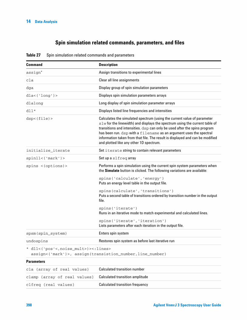
14 Data Analysis
Spin simulation related commands, parameters, and files
Table 27 Spin simulation related commands and parameters
Command Description
assign* Assign transitions to experimental lines
cla Clear all line assignments
dga Display group of spin simulation parameters
dla<('long')> Displays spin simulation parameters arrays
dlalong Long display of spin simulation parameter arrays
dll* Displays listed line frequencies and intensities
dsp<(file)> Calculates the simulated spectrum (using the current value of parameter slw for the linewidth) and displays the spectrum using the current table of transitions and intensities. dsp can only be used after the spins program has been run. dsp with a filename as an argument uses the spectral information taken from that file. The result is displayed and can be modified and plotted like any other 1D spectrum.
initialize_iterate Set iterate string to contain relevant parameters
spinll<('mark')> Set up a slfreq array
spins <(options)> Performs a spin simulation using the current spin system parameters when the Simulate button is clicked. The following variations are available:
spins('calculate','energy') Puts an energy level table in the output file.
spins(calculate','transitions') Puts a second table of transitions ordered by transition number in the output file.
spins('iterate') Runs in an iterative mode to match experimental and calculated lines.
spins('iterate','iteration') Lists parameters after each iteration in the output file.
spsm(spin_system) Enters spin system
undospins Restores spin system as before last iterative run
* dll<('pos'<,noise_mult>)><:lines> assign<('mark')>, assign(transistion_number,line_number)
Parameters
cla {array of real values} Calculated transition number
clamp {array of real values} Calculated transition amplitude
clfreq {real values} Calculated transition frequency
398 Agilent VnmrJ 3 Spectroscopy User Guide

Data Analysis 14
clindex {array of real values}
Index of experimental frequency of a transition
iterate {string of parameters}
Parameters to be iterated
niter {1 to 9999} Number of iterations
slfreq {real values} Measured line frequencies
slw {0.01 to 1e6} Spin simulation linewidth
smaxf {-1e10 to 1e10} Maximum frequency of any simulated transition
sminf {-1e10 to 1e10} Minimum frequency of any simulated transition
sth {0 to 1.00} Minimum intensity threshold
svs {0 to 1e10} Spin simulation vertical scale
Table 27 Spin simulation related commands and parameters (continued)
Command Description
Agilent VnmrJ 3 Spectroscopy User Gui
Commonly used spin simulation global parameters and descriptions:
Table 28 Spin simulation global parameters
Parameter Description
cla and clfreq Make up a table consisting of line numbers assigned by the spin simulation program and the corresponding frequency of a measured line when the intensity of the line is above a threshold value set by the parameter th.
clamp Stores the transition amplitude of calculated transitions when they are above a threshold set by parameter sth.
clindex Index of experimental frequency of a transition.
slfreq List of measured line frequencies.
sminf and smaxf Minimum and maximum frequency limits for calculation of the final simulated spectrum. These should be set before the calculation is performed. If the Initialize Parameter button is used, sminf is initialized to sp, and smaxf is initialized to sp+wp.
sth Minimum intensity threshold above which transitions are listed and included in the simulated spectrum. A typical value is 0.05.
svs Maximum intensity of calculated transitions.
slw Spin simulation line width
dga Displays the file of simulation parameters in the Text Output window of the Process Panel.
de 399

400
14 Data Analysis
The following commands are used to set up files for the “iterative” mode of spin simulation in which the calculated spectrum approximates an experimental spectrum.
m
Table 29 Iterative mode related commands
Command Button Description
spins('iterate') Iterate Performs the simulation in the iterative mode
initialize_iterate Initialize parameters
Selects a default value for the parameter iterate that causes iteration of all parameters.
The string parameter, iterate, contains a list of parameters (separated by commas) to be iterated during iterative spin simulations. Typical value is 'A,B,JAB'.
Initializes the parameter iterate to a string containing parameters appropriate to the current spin system and niter to 20.
cla Clear assigned lines
Clears the file of line assignments used for spin simulation.
dla Show assigned lines
Displays the file containing the line assignments.
dlalong Writes the line assignments to the file spini.la of the current experiment. This command is useful in more complex problems where the text window is too small for the dla display. dlalong displays the file in the text window.
spinll Use Line List Copies the frequency list from the last nll or dll line listing (contained in the parameter llfrq) into the simulation line frequency parameter slfreq. spinll, clears previous line assignments, and runs dla.
spinll(‘mark’) Places the line positions in the file mark1d.out into the parameter slfreq. This is useful for manual line assignment.
assign Assign Lines The nearest calculated transitions are assigned to the lines from a dll or nll listing after spinll places them in slfreq. If a frequency in slfreq exists with a line number, the next entry of the same frequency is assigned a unique line. Optional:Assign positive lines only. Run dll(‘pos’) from the command line first. Only lines transitions greater than sth (typically >0.05 to prevent assignment of extremely small lines) are assigned.
assign(‘mark’) The same as assign, except the file mark1d.out is used instead of the dll listing. Use the cursor and the mark button to place the lines to be assigned in the mark1d.out file. This file is cleared by mark(‘reset’). Use nl to move the cursor to the center of a selected line.
Agilent VnmrJ 3 Spectroscopy User Guide

Data Analysis 14
assign(t#,l#) Assigns a single calculated transition number (t#) to a line from a dll listing (the index is l#). Use assign(t#,0) to remove the calculated transition assignment.
undospins Restores a spin system as it was before the last iterative run. Chemical shifts, coupling constants, and transition assignments are returned to those existing immediately before an iterative spin simulation.
Table 29 Iterative mode related commands (continued)
Command Button Description
Agilent VnmrJ 3 Spectroscopy User Gui
See the descriptions in the VNMR Command and Parameter Reference.
The spins.list file is an output table made by the spin simulation program. This file can be displayed by clicking on the list button. The following files can exist in the current experiment.
Table 30 Spin simulation files
File Description
spini.indata Line assignment input (deleted by spins after iterations are completed) for the spins program.
spini.inpar List of parameters whose values are to be determined by spins('iterate').
spins.inpar List of initial settings of a number of spin simulation parameters.
spini.la Current transition assignments for an iterative spin simulation (produced by the dlalong command).
spins.list Name of the output file. It is located in the current experiment. This file always includes the calculated transitions ordered by frequency.
spins.outdata File of frequencies, amplitudes, and transition numbers from a spin simulation. It is used in calculating the displayed spectrum.
spini.outpar Values of the chemical shifts and coupling constants after an iterative spin simulation.
spini.savela Transition line assignments for iterative spin simulation in a format readable by the macro undospins.
spins.stat Constants related to iteration (deleted by the spins program).
de 401

14 Data Analysis
Deconvolution
402
The software supports the deconvolution of observed spectra into individual Lorentzian and Gaussian lines. Up to 2048 data points from an expansion of an experimental spectrum can be deconvoluted at one time. Up to 25 lines can be fit to this section of the observed spectrum. Each line’s shape can be defined to be Lorentzian, Gaussian, or both.
The following parameters are available for each line:
• Frequency (in Hz) of line
• Intensity of line
• Linewidth (in Hz) at half-height of line
• Gaussian fraction of line: 0.0 (completely Lorentzian) to 1.0 (completely Gaussian)
All parameters can be fit at the same time, or selected parameters can be removed from the fit. In addition, a linear baseline correction is added to the fit to avoid large errors produced by base line offsets.
Deconvolution window and controls
Figure 96 Deconvolution window and controls
Agilent VnmrJ 3 Spectroscopy User Guide

Data Analysis 14
Agilent VnmrJ 3 Spectroscopy User Gui
The Deconvolution window, see Figure 96, provides access to deconvolution functions via the following buttons:
Button Function
Auto Make Line List
Create a line list from the current spectrum and threshold using the nll command
Use Line List Use the current line list as a starting point for deconvolution
Set Mark Add the current cursor position to the mark file
Reset Mark Clear all lines from the mark file
Use Mark Use the current mark list as a starting point for deconvolution
Fit it Perform deconvolution on the selected line list using the fitspec command and display the results
Show Results Display the deconvolution fit results in the Text Output page
Show Fit Spectrum
Display the spectrum calculated by deconvolution
Show Spectrum Fourier-transform the current FID file and display the spectrum
Add/Subtract Enter the add/subtract mode using the FT spectrum and fit spectrum
Plot Fit Spectrum
Plot the deconvolution fit spectrum, FT spectrum, and component analysis using the plfit macro
Deconvolution step-by-step
1 Click File in the main menu.
2 Select Open.
The text window displays a list of directories (entries with a backslash as the last character in the name) and files (if any). The menu (near the top of the screen) displays the pathname of the current directory.
3 Select the top directory (/) from the Look In menu of the File Open dialog.
4 Select /vnmr from the file display.
The text window displays the list of subdirectories.
5 Select fidlib from the list.
6 Double-click the file Proton_01.fid.
The file is retrieved to the current experiment and viewport.
7 Click the Process tab.
de 403

404
14 Data Analysis
8 Select the Default page.
9 Select 32k from the Transform Size menu.
Use a larger Fourier transform size than normal for proper digitalization of the line shape when the spectrum is to be deconvoluted. A typical transform size for deconvolution is 2*np.
10 Click the Transform button.
11 Expand the six-line pattern near 7.6 ppm until it fills the center third of the display, with baseline on both sides.
12 Click the Vert Scale menu on the Default page of the Process folder and select Absolute intensity mode.
The absolute intensity mode is required for deconvolutions, simulations, etc.
13 Click Process in the main menu bar.
14 Select Analyze.
15 Select Deconvolution.
The Deconvolution window opens; see Figure 96 on page 402.
16 Click the Show Spectrum button.
17 Set a threshold that lists exactly six lines.
18 Click the Auto Make Line List button.
19 Click the Use Line List button.
A line list and a file containing starting point for the deconvolution are created. The linewidth of the tallest line on the screen is measured automatically and used as the starting linewidth for the calculation.
20 Click the Fit it button.
The analysis is performed. This particular example is an 18 parameter fit (6 frequencies, 6 intensities, and 6 linewidths). The calculated spectrum is displayed in the graphics window when the analysis is done. Numerical results appear in the Text Output panel of the Process folder. The numerical output should be similar to this:
Number of data points: 660
Final chi square: 32611.957
Total number of iterations: 29
Successful iterations: 29
Digital resolution: 0.152 Hz/point
Agilent VnmrJ 3 Spectroscopy User Guide

Data Analysis 14
Agilent VnmrJ 3 Spectroscopy User Gui
ITERATION HAS CONVERGED
21 Click the Plot fit Spectrum button.
The original spectrum, the calculated spectrum, and each of the component lines are plotted automatically, along with the numerical results of the calculation. At the end of this operation, the original spectrum replaces the calculated one.
22 Click the Show Fit Spectrum button to return to viewing the calculated spectrum.
23 Click the Add/Subtract button to view the original spectrum simultaneously with the calculated one.
24 Click the icon on the graphics tool bar to view the difference between the measured and calculated spectra.
Parameters
line frequency intensity integral Linewidthgaussian fraction
1 3800.740 57.543 45.723 0.506 0.000*
2 3799.480 57.509 44.546 0.493 0.000*
3 3793.290 89.616 116.212 0.826 0.000*
4 3792.020 86.232 102.826 0.759 0.000*
5 3785.870 82.859 63.909 0.491 0.000*
6 3784.610 79.897 59.166 0.471 0.000*
Using mark
It is not always possible to produce a suitable line list for starting a deconvolution. Use the Set Mark button following a previous spectral display (ds program) to provide a starting point. Information from marks made with a single cursor is written to the file mark1d.out and contains only a frequency and intensity. The starting linewidth is taken from the parameter slw. Information from marks made with two cursors, placed symmetrically about the center of each line at the half-height point, is written to the file mark1d.out and contains two frequencies, an intensity and an integral. The starting frequency is taken as the average of the two cursor positions. The starting linewidth is taken as their difference.
de 405

14 Data Analysis
Deconvolution related commands and parameters
406
Table 31 lists the associated commands and parameters with a short description.
Table 31 Deconvolution commands and parameters
Commands Description
dsp<(file)> Display calculated spectrum
fitspec<(<'usell'><,><‘setfreq’>)> Perform spectrum deconvolution (VNMR)
fitspec Perform spectrum deconvolution (UNIX)
mark* Determine intensity of spectrum at a point
plfit Plot deconvolution analysis
setgauss(fraction), setgauss(fraction*) Set a Gaussian fraction for line shape
showfit Display numerical results of deconvolution
usemark Use mark as deconvolution starting point
* mark<(f1_position)><:intensity>, mark<(left_edge,region_width)><:intensity,integral> mark<(f1_position,f2_position)><:intensity> mark<(f1_start,f1_end,f2_start,f2_end)><:intensity,integral,c1,c2> mark<('trace',<options>)><:intensity,integral,c1,c2>, mark('reset')
Parameter Description
slw {0.01 to 1e6} Starting default linewidth for deconvolution calculations.
Table 32 Deconvolution commands, parameters, and buttons
Command or parameter Button Description
fitspec Fit it Performs spectrum deconvolution by fitting experimental data to Lorentzian and/or Gaussian line shapes. fitspec uses data in a file fitspec.inpar as a starting point for the calculation.
fitspec writes a text representation of the spectral data to the file fitspec.indata. The results of the fit are contained in a file after the calculation is finished.
fitspec.outpar format is identical to fitspec.inpar. All lines are set to have a linewidth of slw, and a fixed Gaussian fraction of 0. (See the VNMR Command and Parameter Reference for information about keyword options available with fitspec.)
setgauss Modifies the output of the last deconvolution (fitspec.outpar) and makes it the input for a subsequent analysis (fitspec.inpar), after first modifying the Gaussian fraction.
Agilent VnmrJ 3 Spectroscopy User Guide

Data Analysis 14
setgauss(fraction) Use the format setgauss(fraction) where fraction is the Gaussian fraction of the line shape, a number naturally limited from 0 to 1, for example, setgauss(0.4) to allow this fraction to vary.
setgauss(fraction*) Use the format setgauss(fraction*).Suffix the fraction value (defined the same as above) with an asterisk and enclose the value in single quotes, for example, setgauss('1.0*') to fix the fraction.
Table 33 Deconvolution display and plotting commands and macros
Macro Button Description
showfit Show Results Displays deconvolution results and converts the data to a format suitable for printing.
dsp('fitspec.outpar') Show Fit Spectrum Displays the theoretical spectrum described by the parameters produced by a deconvolution calculation.
plfit Plot Fit Spectrum Produces a complete output plot of a deconvolution analysis, plotting the observed spectrum, the full calculated spectrum, each individual component, as well as the numerical results of the analysis.
Table 32 Deconvolution commands, parameters, and buttons (continued)
Command or parameter Button Description
Agilent VnmrJ 3 Spectroscopy User Gui
The deconvolution program writes these text files into the user’s current experiment directory.
Table 34 Deconvolution files
File name Description
fitspec.inpar Contains the starting parameters (frequency, intensity, linewidth, and Gaussian fraction) for a subsequent fitting operation. Optionally, this file contains the Gaussian fraction of the line shape. Any number followed by an asterisk (*) is held fixed during the calculation. All other parameters are varied to obtain the best fit. Edit this file before deconvolution to set different fixed Gaussian fractions for each line.
fitspec.indata Contains the point-by-point intensity of the spectrum in the region ofinterest displayed when the fitting is begun (the part of the spectrumbetween sp and sp+wp).
fitspec.outpar Contains the final parameters (frequency, intensity, linewidth, andGaussian fraction) after a fit has been done.
mark1d.out Contains the result of a mark operation during a spectral display.By using the Use Mark button, this file may be used as an alternativeto the last line list in setting up initial guesses for a fitting operation.
de 407

14 Data Analysis
Reference Deconvolution Procedures
408
All reference deconvolution is done from the command line. The following is a description of the fiddle program and the procedures for reference deconvolution of 1D and 2D data sets. Table 35 list commands for 1D and 2D variations of the fiddle program.
Fiddle program options
Table 35 Fiddle command and variants
Commands Description
fiddle* Perform reference deconvolution
fiddled* Perform reference deconvolution subtracting alternate FIDs
fiddleu* Perform reference deconvolution subtracting successive FIDs from first
fiddle2d* Perform 2D reference deconvolution
fiddle2D* Perform 2D reference deconvolution
fiddle2dd* Perform 2D reference deconvolution subtracting alternate FIDs
fiddle2Dd* Perform 2D reference deconvolution subtracting alternate FIDs
* (option<,file><,option<,file>><,start><,finish><,increment>)
The fiddle program and its variants, see Table 35, perform reference deconvolution using a reference signal with known characteristics to correct instrumental errors in experimental 1D or 2D spectra. The main command to start the program or any of its variants can take multiple string and numeric arguments:
Syntax:
fiddle(option<,file><,option<,file>><,start><,finish><,increment>)
Arguments:
option can be the following keywords:
'alternate' Alternate reference phase + / − (phase sensitive gradient 2D data).
'autophase' Automatically adjust phase.
'displaycf' Stop at the display of the correction function.
'fittedbaseline' Use cubic spline baseline correction defined by integral regions.
Agilent VnmrJ 3 Spectroscopy User Guide

Data Analysis 14
'invert' Invert the corrected difference spectrum/spectra.
'noaph' Do not automatically adjust zero order phase of the reference region.
'nodc' Do not use dc correction of the reference region.
'nohilbert' Do not use Hilbert transform algorithm. Use the extrapolated dispersion mode reference signal unless 'noextrap' is also used as an option.
'normalise' Keep the corrected spectrum integrals equal to the first spectrum.
'readcf' Read the correction function from file; the argument file must immediately follow 'readcf'.
'satellites' Use the satellites defined in file in the ideal reference region. The file should be in /vnmr/satellites.
'stop1' Stop at the display of the experimental reference FID.
'stop2' Stop at the display of the correction function.
'stop3' Stop at the display of the corrected FID.
'stop4' Stop at the display of the first corrected FID.
'verbose' Show information about processing in the main window.
'writecf' Write the correction function to file. The argument file must immediately follow 'writecf'.
'writefid' Write out the corrected FID to file. If file does not begin with / it is assumed to be in the current working directory.
Agilent VnmrJ 3 Spectroscopy User Gui
file — name of the file used with the 'satellites' and 'writefid' options.
start and finish — indices of the first and last array elements to be processed.
increment — specifies the steps in which the index is to increment. The default is to process the transformed spectra in an array.
Reference deconvolution of 1D spectra
Only spectra that contain a well-resolved reference signal dominated by a single component, not a simple multiplet, are suitable for reference deconvolution.
1 Fourier transform the raw FID with ft, preferably having zero filled (that is, set fn >= 2*np). (If there are sinc wiggles, use wft with gf = at*0.6.)
2 Set the reference line to the chosen signal using the rl command, and then use two cursors on either side of the line to define a region of spectrum that includes all of the
de 409

410
14 Data Analysis
reference signal, plus a little clear baseline but no other signals. This reference region will be used to define the instrumental line shape.
3 Decide what line shape to convert the instrumental line shape to, and set the weighting parameters accordingly. Create a 1-Hz wide Lorentzian by setting lb to 1 and all other weighting parameters to 'n'.
The negative consequence to signal-to-noise ratio penalty for resolution enhancement is 2 Hz wide lb=0, an infinitely sharp line with infinitely poor signal-to-noise is produced. A recommended strategy is to set lb to minus the expected natural linewidth and choose gf to give reasonable S/N. This strategy should convert the instrumental line shape to Gaussian. Resolution enhancement can be obtained by making lb more negative where signals of interest are broader than those of the reference are.
4 Type the fiddle command to carry out the reference deconvolution and display the corrected spectrum. The integral should remain unchanged. Any resolution enhancement will result in an increase in the amplitude of both signal and noise.
5 To save the corrected data, use the option 'writefid' when doing the reference deconvolution. For example, to store the file correctedfid.fid in the current working directory, enter fiddle('writefid','correctedfid').
The options 'writecf'<,file> and 'readcf'<,file> write and read the correction function. Performing reference deconvolution on one FID using fiddle with the 'writecf' option and then use fiddle with 'readcf' to process another FID applies the first correction function to the second FID. Reference deconvolution can be useful for heteronuclear lineshape correction (provided that the spectral widths for the two nuclei are in the ratio of the respective magnetogyric ratios) or for correcting spectra in which a reference signal has been suppressed (for example, an INADEQUATE spectrum can be corrected for lineshape errors by using a correction function derived from the normal carbon spectrum).
Correct a series of spectra in an arrayed or 2D experiment
Use numeric arguments: fiddle(1) corrects spectrum 1, fiddle(2,3) spectra 2 and 3, etc.
Agilent VnmrJ 3 Spectroscopy User Guide

Data Analysis 14
Agilent VnmrJ 3 Spectroscopy User Gui
Common satellites associated reference signals
• 13C satellites
• 29Si satellites
• quartet satellites (normally unresolved) from three-bond coupling to 13C
13C satellites are typically small enough to be ignored in
samples that are not 13C enriched. Referencing requiring high accuracy in which there are strong (for example 29Si) satellites is accomplished by including the satellites in the specified form of the ideal reference signal by using the 'satellites' option.
The /vnmr/satellites directory contains the file TMS with details of the TMS satellite signals. The command fiddle('satellites','TMS') allows for the satellite signals when deconvoluting using TMS as a reference.
The format for satellite files consists of three real numbers in the following order:
• Separation of the satellite line from the parent signal, in Hz (0.5 JXH in the absence of homonuclear coupling).
• Intensity relative to the parent signal (natural abundance divided by the number of satellite lines [usually 2]).
• Isotope shift to high field, in ppm.
For example, the line
corresponds to a pair of satellite signals from a spin-1/2 isotope with an abundance of 4.6%, a coupling to the observed nucleus of 6.6 Hz, and an isotope shift to high field of 0.001 ppm.
Multiple lines in the satellite file account for multiple satellite signals on the parent peak.
Corrected-difference spectroscopy
Use the command fiddled to produce the corrected difference between successive spectra that divides arraydim in half. The difference spectrum is written into the second element of the pair. Because the main aim of reference deconvolution is to optimize the purity of the difference spectrum, the target line shape would be chosen to give the best possible S/N. This method corresponds to choosing a target line shape approximately twice the width of the raw experimental signals of interest. The command fiddleu produces corrected differences between successive FIDs and the first FID.
3.3 0.023 0.001
de 411

14 Data Analysis
Reference deconvolution of 2D spectra
412
The commands fiddle2d, fiddle2D, fiddle2dd, and fiddle2Dd function like the parent fiddle program. Because the principal objective in 2D reference deconvolution is the reduction of t1-noise, ideal line shape parameters are normally chosen for optimum S/N ratio rather than resolution enhancement.
1 Choose fn (preferably with fn>=2*np) and fn1.
2 Type ft to transform the raw data (as mentioned earlier, if there is significant signal left at the end of at, it might be necessary to use wft with gf set).
3 Display the first increment with ds(1), adjust the phase of the reference signal, and use rl to select the reference signal.
In earlier versions of fiddle, it was necessary to create a parameter, phinc, to anticipate the changes in the reference signal phase with increasing evolution time. The current algorithm automatically adjusts the phase (unless the 'noaph' option is selected). Deconvolution will set the reference signal phase as a function of t1 to place the reference signal at frequency rfp1 in f1. Therefore, remember to set rfl1 and rfp1 before using fiddle2D or the f1 frequencies might unexpectedly change.
4 Define the reference region with the two cursors, and then enter the command fiddle2D('writefid',<file>) (or fiddle2Dd if a 2D difference spectrum is required, as with corrected HMBC). The 'writefid' option is essential, because fiddle2D alone does not store the corrected time-domain data. If phase-sensitive gradient-enhanced 2D data is to be processed, alternate FIDs will have opposite phase modulations (that is, the experimental array will alternate N-type and P-type pathways). In such a case, use the 'alternate' option.
The corrected 2D FID data can be read into an experiment and processed as normal after deconvolution is complete. The value of arraydim no longer matches the arrays set if fiddle2Dd has been used and it might be necessary to set the arguments to wft2d explicitly rather than using wft2da.
Agilent VnmrJ 3 Spectroscopy User Guide

Data Analysis 14
References
Agilent VnmrJ 3 Spectroscopy User Gui
Further information on reference deconvolution can be found in the following literature:
Taquin, J. Rev. Physique App. 1979, 14, 669.
G. A. Morris, J. Magn. Reson. 1988, 80, 547.
G. A. Morris, D. Cowburn, MRC 1989, 27, 1085.
G. A. Morris, H. Barjat, T. J.Horne, Prog. NMR Spectrosc. 1997, 31, 197.
A. Gibbs, G. A. Morris, J. Magn. Reson. 1991, 91, 77.
A. Gibbs, G. A. Morris, A. Swanson, D. Cowburn, J. Magn. Reson. 1983, 101, 351–356.
D. N. Rutledge Ed., Signal Treatment and Signal Analysis in NMR, Chapter 16. Elsevier Science, 1996.
de 413

14 Data Analysis
Addition and Subtraction of Data
414
Individual 1D spectra, FIDS, individual 1D traces from nD data sets, or spin simulated spectra can be added and subtracted. The process uses one experiment to display the results and experiment 5 as the add/subtract buffer file. Any data in experiment 5 (exp5) is overwritten.
Menu for add and subtract
Access the Add / Subtract experiments from the main menu as follows:
1 Click Process in the main menu.
2 Select Add and Subtract 1D Data.
The following sub-menu items are displayed:
Clears buffer (experiment 5): Creates experiment 5 and places current spectrum in experiment 5.
Add Second Spectrum into Buffer: Adds current spectrum (algebraically) to data in experiment 5.
Interactive add/subtract toolbar
The Interactive Add/Subtract toolbar has the following buttons (the labels on some buttons change depending on the current mode):
Each button, name (tool tip), and function is listed in Table 36.
Table 36 Add/subtract toolbar buttons
Button Name Description
Box Box is shown when the display is in the cursor mode. Click to change to the box mode with two cursors.
Cursor Cursor is shown when the display is in the box mode. Click to change to the cursor mode.
Select Selects the current, addsub, or result mode. Text in the field next to active matches the color of the spectrum. Arrow colors:Green — current mode (spectrum) is selectedYellow — addsub mode (spectrum) is selectedBlue — result mode (spectrum) is selected
Expand The third button is labeled Expand or Full, depending on the selected mode, box or cursor. When Expand appears the box mode is active, and clicking on this button expands the area between the cursors.
Agilent VnmrJ 3 Spectroscopy User Guide

Data Analysis 14
Agilent VnmrJ 3 Spectroscopy User Gui
Full When Full appears, the cursor mode is active, and clicking on this button displays the full area.
sp wp Adjusts the start and width of the active spectrum.
sub The fifth button is labeled sub, min, or add. When sub appears, clicking on the button makes the result spectrum to be the difference between the current and the add/sub spectra.
min When min appears, clicking on the button makes the result spectrum to be a minimum intensity of either the current or the add/sub spectra.
add When add appears, clicking the button makes the result spectrum to be a sum of the current and the add/sub spectra.
save Saves the result spectrum in the add/sub spectrum in experiment 5 and returns to the last menu.
return Returns to the last menu without saving the result.
Table 36 Add/subtract toolbar buttons (continued)
Button Name Description
Interactive add/subtract
Interactive add/subtract is a multi-step process using the menu system to call the addi command and uses exp5 as an add/subtract buffer file. Two spectra can be interactively added or subtracted using the menu add and subtract tools on the add/subtract tool bar; see Table 36. Both horizontal displacement and vertical scale of the two spectra to be added or subtracted are under interactive control. Spectra that can be phased can be phased independently. The result can be manipulated using any of the standard software (for example, the command pl), including further interactive add/subtract with another data set.
To add and subtract spectra
1 Select any available experiment or create a new experiment. Do not use or create experiment 5.
2 Click File in the main menu.
de 415

416
14 Data Analysis
3 Select Open.
The text window displays a list of directories (entries with a backslash as the last character in the name) and files (if any). The menu (near the top of the screen) displays the pathname of the current directory.
4 Select the top directory (/) from the Look In menu of the File Open dialog.
5 Select /vnmr from the file display.
The text window displays the list of subdirectories.
6 Select fidlib from the list.
7 Select an arrayed 1D data set such as dept.fid.
8 Click the Transform button on the action bar.
9 Click Process in the main menu.
10 Select Add and Subtract 1D Data.
11 Select Clear Buffer and Add Current Spectrum from the sub-menu.
Clears buffer (experiment 5): Creates experiment 5 and places current spectrum (spectrum 1) in experiment 5.
12 Select the spectrum to add or subtract from the first spectrum by doing either of the following:
• Click either the or until the desired spectrum is displayed.
• Type ds(#) where # is the number of the spectrum in the array.
13 Select Add and Subtract 1D Data.
14 Select Add Second Spectrum into Buffer from the sub-menu.
The default operation is to add the spectra. The current spectrum (spectrum 2) is added algebraically to data in experiment 5 (spectrum 1) and displays the three spectra as shown in Figure 97.
Agilent VnmrJ 3 Spectroscopy User Guide
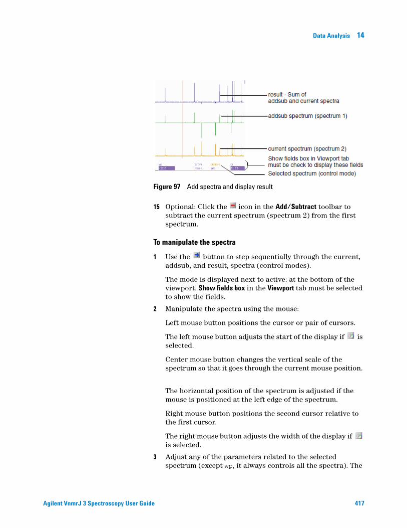
Data Analysis 14
Agilent VnmrJ 3 Spectroscopy User Gui
15 Optional: Click the icon in the Add/Subtract toolbar to subtract the current spectrum (spectrum 2) from the first spectrum.
To manipulate the spectra
1 Use the button to step sequentially through the current, addsub, and result, spectra (control modes).
The mode is displayed next to active: at the bottom of the viewport. Show fields box in the Viewport tab must be selected to show the fields.
2 Manipulate the spectra using the mouse:
Left mouse button positions the cursor or pair of cursors.
The left mouse button adjusts the start of the display if is selected.
Center mouse button changes the vertical scale of the spectrum so that it goes through the current mouse position.
The horizontal position of the spectrum is adjusted if the mouse is positioned at the left edge of the spectrum.
Right mouse button positions the second cursor relative to the first cursor.
The right mouse button adjusts the width of the display if is selected.
3 Adjust any of the parameters related to the selected spectrum (except wp, it always controls all the spectra). The
Figure 97 Add spectra and display result
de 417

418
14 Data Analysis
spectrum can be phased, scaled, or shifted relative to the other spectrum.
4 Click Process in the main menu bar.
5 Select Analyze.
6 Select Deconvolution.
The Deconvolution window opens, see Figure 96 on page 402.
7 Click the Add / Subtract button to display the resulting spectra and return to the interactive add and subtract mode.
8 Optional: Save the addsub spectrum after all the manipulation of the data has been completed if further operations, plotting, adding another spectrum, etc. are required.
a Click to save the addsum spectrum into experiment 5. Spectrum 1, which was in the add/subtract buffer of experiment 5 is overwritten by the sum or difference spectrum. The interactive Add / Subtract routine exits.
b Save the result in experiment 5 to a file or move it to another available experiment.
Non interactive add/subtract
The non interactive add / subtract procedure is run from the command line. The buffer (exp5) is first cleared using clradd. Different FIDs or spectra are then added to or subtracted from the accumulating total by the commands add, sub, spadd, and spsub.
Adding and subtracting FIDs
The add and sub commands add and subtract the last displayed or selected FID to and from the contents of the add/subtract experiment. An optional argument allows the FID to first be multiplied by a multiplier (the default is 1.0). The parameters lsfid and phfid can be used to shift or phase rotate the selected FID before it is combined with the data in the add/subtract experiment.
A multi-FID add/subtract experiment with FIDs 1 and 2 is created with the add or sub command using the keyword 'new' as follows:
1 Create the add/subtract experiment with a single FID by entering the following commands from some experiment:
clradd select(1) add
Agilent VnmrJ 3 Spectroscopy User Guide

Data Analysis 14
Agilent VnmrJ 3 Spectroscopy User Gui
2 Make the add/subtract experiment contain an array of two FIDs corresponding to the original FIDs 1 and 2 by entering:
select(2) add('new')
Entering the following makes the add/subtract experiment contain a single FID that is the sum of the original FIDs 1 and 2 instead of an array:
select(2) add
The arraydim parameter may need to be updated after constructing a multi-FID add/subtract experiment.
3 Type jexp5 to join exp5.
4 Use setvalue('arraydim',numFIDs,'processed') to place numFIDs of FIDs into exp5.
The number of FIDs in the experiment is numFIDs.
Example:
setvalue('arraydim',12,'processed') places 12 FIDs into exp5.
Individual FIDs in a multi-FID add/subtract experiment can be added to and subtracted from one another. The add and sub commands without the keyword 'trace' adds or subtracts from the first FID in the add/subtract experiment. Adding the keyword 'trace' followed by the required index number selects specific FID to be the target of the add/subtract.
Example:
select(4) add('trace',6) takes the fourth FID from the current experiment and adds it to the sixth FID in the add/subtract experiment.
The FID must already exist in the add/subtract experiment by using an appropriate number of add('new') or sub('new') commands when using the keyword 'trace'.
de 419

14 Data Analysis
Adding and subtracting spectra
420
Non-interactive spectral addition and subtraction uses the spadd and spsub commands. The last displayed or selected spectrum is added to (spadd) or subtracted from (spsub) the current contents of the add/subtract experiment.
Each spectrum can be optionally multiplied and shifted using the multiplier and shift arguments, respectively. For example, entering spadd(0.75,10) multiplies the spectrum by 0.75 and shifts the spectrum by 10 to the left. A positive shift value shifts the spectrum being added or subtracted to higher frequency, or to the left. A negative shift value shifts the spectrum being added or subtracted to lower frequency, or to the right. To shift a spectrum without multiplying it, use a multiplier of 1.0.
A multi-element add/subtract experiment with spectra 1 and 2 is created with the spadd or spsub command using the keyword 'new' as follows:
1 Create the add/subtract experiment with a single spectrum by entering the following commands from some experiment:
clradd select(1) spadd
2 Make the add/subtract experiment contain an array of two spectra corresponding to the original spectra 1 and 2 by entering:
select(2) spadd('new')
Entering the following makes the add/subtract experiment contain a single spectrum that is the sum of the original spectra 1 and 2 instead of an array:
select(2) spadd
Individual spectra in a multi-element add/subtract experiment can subsequently be added to and subtracted from. The spadd and spsub command without the keyword 'trace' adds to or subtracts from the first spectrum in the add/subtract experiment. Adding the keyword 'trace' followed by the index number of the spectrum selects that spectrum to be the target of the add/subtract. Entering select(4) spadd('trace',6) takes the fourth spectrum from the current experiment and adds it to the sixth spectrum in the add/subtract experiment.
The indexed spectrum must already exist in the add/subtract experiment by using an appropriate number of spadd('new') or spsub('new') commands with the 'trace' argument. Join experiment 5 (jexp5) and use the normal spectral display (for example, ds) and plotting commands to examine the results.
Agilent VnmrJ 3 Spectroscopy User Guide

Data Analysis 14
Add / Subtract related commands and parameters
Agilent VnmrJ 3 Spectroscopy User Gui
The add/subtract experiment related commands are listed in Table 37 and parameters are listed in Table 38.
Table 37 Add/Subtract related commands
Commands Description
add* Add current FID to add/subtract experiment
addi Start interactive add/subtract mode
clradd Clear add/subtract experiment
jexp1, ..., jexp9999 Join existing experiment
select* Select a spectrum or 2D plane without displaying it
setvalue* Set value of a parameter in a tree
spadd* Add current spectrum to add/subtract experiment
spmin Take minimum of two spectra in add/subtract experiment
spsub* Subtract current spectrum from add/subtract experiment
sub* Subtract current FID from add/subtract experiment
*add<(multiplier<,'new'>)>, add('new'), add('trace',index)select<('next'|'prev'|selection)><:index>,select<(<'f1f3'|'f2f3'|'f1f2'><,'proj'><,'next'|'prev'|plane>)><:i>setvalue(parameter,value<,index><,tree>)spadd<(multiplier<,shift>)>, spadd('new'), spadd('trace',index) spsub<(multiplier<,shift>)>, spsub('new'),spsub('trace',index) sub<(multiplier<,'new'>)>, sub('new'), sub('trace',index)
Table 38 Add/Subtract related parameters
Parameters Description
arraydim {number} Dimension of experiment
lsfid {'n',-fn/2 to ni or fn/2} Number of complex points to left-shift np FID
phfid {'n',-360 to 360, in degrees} Zero-order phasing constant for np FID
de 421
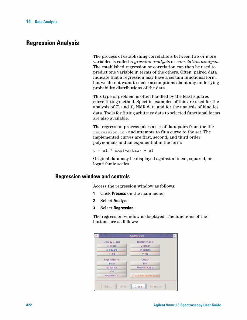
14 Data Analysis
Regression Analysis
422
The process of establishing correlations between two or more variables is called regression analysis or correlation analysis. The established regression or correlation can then be used to predict one variable in terms of the others. Often, paired data indicate that a regression may have a certain functional form, but we do not want to make assumptions about any underlying probability distributions of the data.
This type of problem is often handled by the least squares curve-fitting method. Specific examples of this are used for the analysis of T1 and T2 NMR data and for the analysis of kinetics data. Tools for fitting arbitrary data to selected functional forms are also available.
The regression process takes a set of data pairs from the file regression.inp and attempts to fit a curve to the set. The implemented curves are first, second, and third order polynomials and an exponential in the form:
y = a1 * exp(-x/tau) + a3
Original data may be displayed against a linear, squared, or logarithmic scales.
Regression window and controls
Access the regression window as follows:
1 Click Process on the main menu.
2 Select Analyze.
3 Select Regression.
The regression window is displayed. The functions of the buttons are as follows:
Agilent VnmrJ 3 Spectroscopy User Guide

Data Analysis 14
Agilent VnmrJ 3 Spectroscopy User Gui
Button group Function
Display x-axis buttons:
x-linear Display output with a linear x-axis
x-square Display output with a quadratic x-axis
x-log Display output with a logarithmic x-axis
Display y-axis buttons:
y-linear Display output with a linear y-axis
y-square Display output with a quadratic y-axis
y-log Display output with a logarithmic y-axis
Regression fit buttons:
linear Perform a linear regression analysis
quadratic Perform a quadratic regression analysis
cubic Perform a cubic regression analysis
exponential Perform an exponential regression analysis
Output buttons:
Plot Plot the regression analysis
Show fit output Display regression output
Create interactive input The program displays a series of prompts requesting input
Regression, step-by-step using the regression window
1 Click Create interactive input button.
The program displays a series of prompts requesting the axis label titles and the data pairs.
a Enter an X and Y pair separated by a space.
b Enter the next X and Y pair.
c Finish the data set by pressing the Enter key.
d Respond to the prompt and press y to enter another data set or n to end the data entry.
The file regression.inp is created in the correct format when all the data is input and the data points and axis are displayed on the screen.
2 Click any one of the buttons Display x-axis or Display y-axis group.
de 423

424
14 Data Analysis
Each button scales the display and shows either the x or y axis as labeled on the button.
3 Click one of the buttons in the Regression fit to select a fitting routing. These buttons include displaying the results using expl.
Figure 98 on page 425 shows quadratic fittings for the data set in Table 39.
Data is written to the regression.inp and analyze.out files. Contents of these files are explained in “Contents of “regression.inp” file” on page 430.
Fitting routine Analyze option Button in regression fit group
linear 'poly1' Linear
quadratic 'poly2' Quadratic
cubic 'poly3' Cubic
exponential curve 'exp' Exponential
Table 39 Sample data table
Data set 1
X value Y value
0.0 5.0
1.0 9.0
2.0 12.0
3.0 20.0
4.0 33.0
5.0 42.0
Data set 2
X value Y value
0.0 20.0
1.0 22.0
2.0 27.0
3.0 29.0
4.0 37.0
5.0 45.0
Agilent VnmrJ 3 Spectroscopy User Guide

Data Analysis 14
Agilent VnmrJ 3 Spectroscopy User Gui
4 Click the Plot button to plot the analysis.
The scale automatically to show all points (if possible).
5 Click the Show fit output button to show the results of the analysis in the Text Output window.
Figure 98 Display of regression fittings
Regression, step-by-step using the command Line
1 Write and save the text file regression.inp that contains the data pairs to analyze. The next section describes the format of this file. Create it by one of the following methods:
• Enter rinput on the command line.
• The program displays a series of prompts requesting the axis label titles and the data pairs. The file regression.inp is created in the correct format when all the data is input. The data can be corrected using a text editor after the program writes the file.
• Use a text editor such as vi or textedit.
• Create a MAGICAL II macro for this purpose.
2 Enter the command expl('regression') for single data sets or expl('regression', line#, line#,...) for multiple data sets.
The expl command uses the values in the regression.inp file to display a graph of the data points. It also creates the files analyze.inp (needed by analyze to run the analysis) and expl.out (display information for expl).
de 425

426
14 Data Analysis
Optional: Use the poly0 macro to calculate and display (as horizontal lines) the mean of the data in the file regression.inp.
3 Enter analyze('expfit','regression',option,'list') the command line.
The fitting routine choices for option are 'poly1', 'poly2', 'poly3', or 'exp'.
The program expfit is called by this usage of the analyze command.
expfit creates the files analyze.out (used by expl to display the results) and analyze.list (a table of results).
4 Enter expl to see the results as a graph.
Figure 98 on page 425 shows quadratic fittings for the data given in the example of the regression.inp file in the next section.
5 Enter pexpl page to plot one data set or enter pexpl(index#,index#,...) to plot multiple data sets.
Both expl and pexpl set the scale automatically to show all points (if possible).
6 Optional.
Enter the scalelimits macro to set limits for the scales using one of the following:
• Enter scalelimits with no argument to start an interactive process that prompts for the four scale limits.
• Enter scalelimits(x_start,x_finish, y_start,y_finish) with limits for the x-axis and y-axis as arguments.
The limits are retained as long as an expl display is retained. Enter autoscale to return to automatic scaling by expl.
7 Enter cat(curexp+'/analyze.list’) to show the results of the analysis in the Text Output panel.
Fitting routine Analyze option
linear 'poly1'
quadratic 'poly2'
cubic 'poly3'
exponential curve 'exp'
Agilent VnmrJ 3 Spectroscopy User Guide

Data Analysis 14
Contents of “analyze.out” file
Agilent VnmrJ 3 Spectroscopy User Gui
The data input file is analyze.out, except for regression when the input file is regression.inp. The file expl.out saves certain display and plot parameters.
Values can be 2048 points maximum from a data set, 2048 points maximum from all sets displayed/plotted, 8 data sets maximum displayed, and 128 data sets maximum are read.
The following is an example of analyze.out. Numbers identify lines in the example and are not part of the actual file:
Curve types supported are listed in Table 40
Line number
1 exp 7 regression
2 D1 C0 C1 C2
3 1 5 linear linear
4 Exponential Data Analysis
time
amp
5 NEXT 5
6 1 -248.962 22.8025 226.157
7 2 4
3 9
4 16
5 25
6 36
Table 40 Curve type
Type Function Functional form
0 T1/T2 (a0 – a2)*exp(–t/a1) + a2
1 Increasing kinetics a0*exp(–t/a1) + a2
2 Decreasing kinetics –a0*exp(–t/a1) + a2 + a0
3 Diffusion a0*exp(–D1*uu) + a2*exp(–a1*D1*uu) where uu=C0+C1*t+C2*t2
4 None No theoretical curve (use 'link')
5 Linear a0 + a1*t
de 427

428
14 Data Analysis
The following is a description of the numbered parts of this file:
Next is an example of regression.inp file for generalized curve fitting.
6 Quadratic a0 + a1*t + a2*t2
7 Exponential a0 * exp(–t/a1) + a2
8 Contact time (a3 –(a3 – a0)*exp(–t/a1)) *exp(–t/a2) + a0
9 Cubic a0 + a1*t + a2*t2 + a3*t3
Line number Description
1 The keyword exp is followed by a number for a curve type from Table 40 Curve Type 40.
The keyword regression, if present, indicates regression output.
2 Floating point constants D1, C0, C1, and C2, if present, are used only with the diffusion function (curve type 3).
3 An integer for the number of data sets (curves), followed by an integer for the number of data point pairs in the set. For regression, the words are scale types for the x and y axes: linear, square, and log.
4 Title line. Use No Title when a title is not desired. Two additional text lines for the x and y axis titles are present in output from regression.
5 The keyword NEXT identifies the start of a data set, and the integers that follow give the number of data point pairs in the data set.
6 The first integer specifies the number (usually 1) of the data point symbol used for the data set. The next three integers are the coefficients a0, a1, and a2 (see Table 40) and must all be present, even for functions that do not use all three (for example, first-order polynomial). If a particular number is not appropriate, put any number there. a3 must be also be present for cubic and contact time functions (curve types 7 and 8).
7 Data point pairs in the set.
Line number
1 time
2 amp
3 0 0
Table 40 Curve type (continued)
Type Function Functional form
Agilent VnmrJ 3 Spectroscopy User Guide

Data Analysis 14
Agilent VnmrJ 3 Spectroscopy User Gui
Description of this example:
The final example uses the 'file' argument to the expl command:
4 NEXT
5 2.000000 4.000000
3.000000 9.000000
4.000000 16.000000
5.000000 25.000000
6.000000 36.000000
Line number Description
1 Line with text for x-axis label displayed by expl('regression').
2 Line with text for y-axis label (line must not be too long, usually less than 20 characters). The first non-blank character must not be a digit.
3 Line containing an integer for the number of data sets followed by another integer for the number of pairs per data set. Both values are 0 if the number of pairs is variable.
4 A line beginning with the keyword NEXT is inserted at the start of each data set when the number of pairs per peak is variable.
5 The data pairs, listed one pair to a line.
Line number
1 exp 4
2 1 5
3 time
4 1 0 0 0
5 2 4
3 9
4 16
5 25
6 36
de 429

430
14 Data Analysis
Description of this example:
Line number Description
1 Keyword exp followed by curve type number
2 Number of data sets, followed by number of data point pairs
3 Title
4 Data point symbol number, followed by three coefficients
5 Data point pairs in the set
Contents of “regression.inp” file
The data input text file regression.inp contains a listing of axis labels and data pairs. The data file can contain up to 128 data sets. Data sets are selected by expl indexes (up to 6, depending upon length of data sets) with a default to the beginning data sets. The analysis is limited to 1024 data points, with the first part of larger data sets selected.
The following is an example of a regression.inp file that shows the format used. Numbers identify lines in the example and are not part of the actual file:
Line number
1 time
2 temp
3 0 0
4 NEXT
5 0.000000 5.000000
1.000000 9.000000
2.000000 12.000000
3.000000 20.000000
4.000000 33.000000
5.000000 42.000000
4 NEXT
5 0.000000 20.000000
1.000000 22.000000
2.000000 27.000000
3.000000 29.000000
Agilent VnmrJ 3 Spectroscopy User Guide

Data Analysis 14
Agilent VnmrJ 3 Spectroscopy User Gui
Description of this file:
4.000000 37.000000
5.000000 45.000000
Line number Description
1 X-axis label for display by expl('regression'). The label is optional. If used, the first non-blank character in the label must not be a digit.
2 Y-axis label for display by expl('regression'). The label is optional. If used, it must be less than about 20 characters and the first non-blank character in the label must not be a digit.
3 If the number of pairs per data set is fixed, this line contains an integer for the number of data sets, followed by another integer for the number of data pairs per data set. If the number of pairs per data set is variable (as in this example), both integers are set equal to 0.
4 If the number of pairs per data set is variable, a line with the word NEXT is inserted at the start of each data set.
5 Data pairs, one to a line, are listed for each data set, in this order:
first pair of first set
second pair of first set
third pair of first set
. . .
first pair of second set
second pair of second set
Regression commands
Table 41 lists the commands associated with regression analysis.
Table 41 Regression commands
Commands Button Description
analyze* Any of the buttons in the Regression fit group.
Generalized curve fitting in regression mode
autoscale Any of the buttons in the Output group.
Resume autoscaling after limits set by scalelimits
de 431

432
14 Data Analysis
expfit* Any of the buttons in the Regression fit group.
Make least-squares fit to exp. or poly. curve (Linux)
expl<(<options,> line1,...>)>
Any of the buttons in the Display x-axis or Display y-axis group
Display exponential or polynomial curves
pexpl<(<options,> line1,...>)>
Plot Plot exponential or polynomial curves
poly0 Display mean of data in regression.inp file
rinput Create iterative input
Input data for regression analysis
scalelimits* Any of the buttons in the Output group.
Set limits for scales in regression
* analyze('expfit',xarray<,option,option,...>) expfit options <analyze >analyze.list scalelimits(x_start,x_end,y_start,y_end)
Table 41 Regression commands (continued)
Commands Button Description
Agilent VnmrJ 3 Spectroscopy User Guide

Data Analysis 14
Cosy Correlation Analysis
Cosy data chemical shift analysis window and controls
Agilent VnmrJ 3 Spectroscopy User Gui
Analysis of COSY Data Step-by-Step
1 Process and display a COSY data set.
2 Click Process from the main menu.
3 Select Analyze.
4 Select Cosy Correlations…
Opens Cosy Correlations window if current viewport contains an appropriate data set.
5 Click the Create 2D Line List button to create a line list for the COSY data set.
6 Click the Find Correlations button display the correlations of the COSY data set on the screen.
7 Optional:
Click the Redisplay button to redisplay a normal interactive 2D contour map and make any changes or adjustments to the data as needed. Start over again at step 4.
Button Function
Create 2D Line List Write a 2D line listing to the file ll2d.out and displays the results in the Text Output panel.
Find Correlations Analyze the current 2D line listing and display the results on the screen.
Redisplay Display an interactive 2D contour map.
Plot Correlations Analyze the current 2D line listing and plot the results.
Plot Contours Plot the 2D contours.
Plot Page Send plot to the printer.
de 433

434
14 Data Analysis
8 Click the Plot Correlations button to create plot of the line list for the COSY data set.
9 Click the Plot Contours button to create a contour plot of the COSY data set.
10 Click the Plot Page button to send the plot to the printer.
Agilent VnmrJ 3 Spectroscopy User Guide

Data Analysis 14
Chemical Shift Analysis
Agilent VnmrJ 3 Spectroscopy User Gui
Chemical shifts are analyzed using the commands in Table 42. These commands write a list of chemical shifts to the file pcss.outpar.
Table 42 Chemical shift analysis commands
Commands Description
do_pcss Calculate proton chemical shifts spectrum
pcss Calculate and show proton chemical shifts spectrum
de 435

436
14 Data Analysis
Agilent VnmrJ 3 Spectroscopy User Guide

Agilent VnmrJ 3 SpectroscopyUser Guide
15Pulse Analysis
Pandora’s Box 438
Pulse Shape Analysis 455
This chapter provides information on the Locator and File Browser.
437Agilent Technologies

15 Pulse Analysis
Pandora’s Box
438
Pandora’s Box (Pbox) software creates shape pattern files for experiments involving shaped RF pulses, composite pulses, decoupling and mixing patterns, adiabatic RF sweep waveforms, and pulsed field gradient shapes. Pbox provides the parameters (pulse width, power, dmf, dres, etc.) when the shape files are created, and this information can be extracted from Pbox shape files by macros or directly within pulse sequences. More than 160 different shapes are available from the Pbox library.
Create a new waveform
1 Open the Pbox window to access the tools for creating waveforms.
2 Click Edit on the menu bar.
3 Select New Pulse Shapes.
The Pbox window opens.
4 Click the Make Waveform tab.
5 Click the New Waveform button and the tools for creating a wave form are displayed in the Pbox window, see Figure 99.
6 Select the desired shape from the Shape type menu.
Figure 99 Pbox make waveform tab
Agilent VnmrJ 3 Spectroscopy User Guide

Pulse Analysis 15
Agilent VnmrJ 3 Spectroscopy User Gui
7 Select the desired shape name from the Shape name menu. The Shape name choices depend on the selected Shape type.
8 Set the Reference pw90 and Reference power.
9 Set the waveform selection region as follows:
a Display a spectrum.
b Select a selective excitation band using two cursors.
c Click Select from the spectrum button. This sets the Bandwidth, Pulse length, and Frequency offset from the cursors.
d Optional: Explicitly enter Bandwidth, Pulse length, and Frequency offset.
10 Click Add Waveform. The Wave # field is updated and the Make It! button becomes active.
11 Add additional waveform shapes into a waveform by repeating steps 4 through 8 (above). The Wave # field updates for each selective shape added to the waveform.
12 Enter a name for the shape in the Shape file name entry box.
The field contains a default file name of Pbox.
13 Enter any Additional Options (see Table 44).
14 Click Make It! to generate and save the shape file.
15 Request simulations, see Figure 100, as follows:
a Click the Show XY or Show Z option button.
b Select Show spectrum to show the spectrum.
c Click Simulate. The simulation is displayed in the graphics window.
Figure 100 Shaped Pulse Simulations Reference Spectrum
de 439

15 Pulse Analysis
Update parameter values
440
Update the parameter values used by the waveform into the experimental parameters as follows:
1 Click the Update Parameters tab, see Figure 101.
2 Enter a shape file name in the entry box.
3 Click Read parameter values to read parameter values from the Pbox shape file.
4 Enter names for the parameters or use the suggested defaults for the waveform.
5 Click Reset parameter names to reset the parameter names to the default values, if desired.
6 Click Set parameter values into experiment to set the parameter values into the experimental parameters.
Parameters that do not exist are not set in the experiment. Parameter limits are not selected (especially for pulse width) — select them.
Figure 101 Pbox update parameters
Agilent VnmrJ 3 Spectroscopy User Guide

Pulse Analysis 15
Calibrating the RF field
Agilent VnmrJ 3 Spectroscopy User Gui
In the input, provide the RF field calibration data ref_pwr and ref_pw90 to obtain the pulse calibration numbers in the Pbox output before waveform creation. Ensure that the RF field has been calibrated for the length of the 90° pulse at a given power level.
The RF field can be calculated at any power using spectrometers with linear amplifiers such as those on Agilent NMR spectrometer systems. Maximum accuracy for the calibration is obtained when the calibration is made as close as possible to the field used in the experiment. Provide approximate calibration data and use cal as an output file name for Pbox to permit an estimate of the RF field. No waveform is created and only the calibration results appear in the output.
Creating waveforms by macros
Pbox macros provide useful tools for customizing NMR experiments. The simplest way to create a shape is by using the pxshape macro. For example, a single band excitation pulse using the E-BURP-1 shape, covering 400 Hz, and shifted off-resonance by –880 Hz from the carrier frequency (middle of the spectrum) can be created and stored in the alpha.RF file as follows:
pxshape('eburp1 400.0 -880','alpha.RF')
The following steps are necessary to create multiply-selective pulses. Use the cursors if the spectrum of interest is on the screen. The parameters ref_pwr90 and refpwr must be present and set correctly in the current parameter set.
1 Type opx('hadamard.RF') to open the Pbox.inp file and write the file header.
2 Select an excitation band using cursors.
3 Type selex('rsnob').
4 Select the second excitation band using cursors.
5 Type selex('rsnob').
6 Repeat steps 2 to 5 as many times as needed.
7 Type cpx to close the Pbox.inp file.
8 Type dshape to display the last created shape.
de 441

442
15 Pulse Analysis
The following set of macros is used if an experimental spectrum is not available. The parameters ref_pwr90 and refpwr must be present and correctly set in the current parameter set.
1 Type opx('myshape') to open Pbox and provide a file name.
2 Type setwave('sech 400.0 -880.0') to select first band at –880 Hz.
3 Type setwave('sech 400.0 1240.0') to select second band at 1240 Hz.
4 Type cpx(ref_pw90, ref_pwr) to close Pbox.
5 Type dshape to display the shape file.
The pbox_pw and pbox_pwr macros are used to load the parameters of the last created shape file into the current experiment:
pbox_pw:selpw
pbox_pwr:selpwr
Alternatively, the calibration data is directly retrieved from the shape file provided as an argument to the pbox_dmf and pbox_dres macros:
pbox_dmf('ccdec.DEC'):dmf
pbox_dres('ccdec.DEC'):dres
where ccdec.DEC is the name of the decoupling shape file.
The excitation profile of shaped pulses is verified using the Pbox Bloch simulator. The parameters ref_pwr90 and refpwr must be present and set correctly in the current parameter set.
1 Type opx to open Pbox.
2 Type setwave('iburp2 400.0 -880') to select first band at –880 Hz.
3 Type setwave('iburp2 400.0 1240.0') to select second band at 1240 Hz.
4 Type pbox_rst to reset par-s and write comments.
5 Type pboxpar('name','test.DEC') to define the output file name.
6 Type pboxpar('bsim','y') to activate the Bloch simulator.
7 Type cpx to close Pbox.
8 Type dshape to display the shape file.
9 Type dprofile('z') to display inversion (Mz) profile.
Agilent VnmrJ 3 Spectroscopy User Guide

Pulse Analysis 15
Agilent VnmrJ 3 Spectroscopy User Gui
Pbox reads the corresponding wave file in the wavelib directory to determine whether the waveform being created is a 90° excitation pulse or a 180° inversion pulse, and the type of wave form required (.RF,.DEC, or.GRD). Pbox can be forced to change the waveform type by providing the required extension to the output shape file name. Modify wave files by copying it into the local user wavelib and editing the text file as required. See “Pbox commands using a terminal” on page 453, for a more complete description of macros.
Creating waveforms in an operating system terminal window
Creating waveforms using an operating system terminal window can be more convenient in some cases:
> Pbox
The name of the output shape file is passed as an argument:
> Pbox filename
The input data are typically stored in the Pbox.inp file in your vnmrsys/shapelib directory and are modified using standard text editors. Alternatively, most of the necessary data can be provided as arguments to the Pbox command. For example,
> Pbox myfile -w "eburp1 480 -1200" -p 40 -l 104
generates an E-BURP-1 excitation pulse covering 480-Hz-wide band and shifted –1200 Hz off-resonance using for calibration 104 μs pw90 at 40 dB power level and stored in myfile.RF. Note that the name of the output shape file is always passed as the first argument.
Several other options are accepted by Pbox. For example, -b activates the Bloch simulator, -c calibrates the waveform without creating a shape file, and -o print out the available options. For more information, see “Pbox commands using a terminal” on page 453.
Pbox file system
Information about the waveform to be created (for example, calibration data, output file name, excitation band definition) is stored in the Pbox.inp text (ASCII) file in the user directory vnmrsys/shapelib. This file is generated whenever Pbox menus or macros are used or created by using one of the standard text editors.
Any shape file can consist of one or several shapes that are combined into a single waveform. Each excitation band is
de 443

444
15 Pulse Analysis
defined by a wave definition string (a string of wave variables enclosed between delimiters {and}). There is an unlimited number of wave definition strings in a single Pbox.inp file. In order to simplify the input file format, the wave variables are entered without names in a strongly predefined order:
sh bw(/pw) ofs st ph fla trev d1 d2 d0 wrap
The following table describes each of the variables.
The order of parameters is listed in descending order of importance. Rarely used parameters can be omitted or defaulted by assigning a value of n (not used). The following examples are valid wave definition strings.
sh Shape name as stored in wavelib
bw(/pw) Bandwidth in Hz, or pulsewidth in sec, or both
ofs Offset from transmitter offset or carrier in Hz
st Spin status (0 for Mz or 1 for Mxy)
ph Phase or phase cycle
fla Flip angle
trev Time reversal flag
d1 Prepulse delay
d2 Postpulse delay
d0 Delay before the pulse
wrap Wraparound parameter
{qsneeze} q-SNEEZE pulse applied on resonance. The pulse length will be internally defaulted to 5 ms.
{G3 800} G3 pulse covering bandwidth of 800 Hz and applied on-resonance
{sech 400/0.05 -1200} 50 ms long hyperbolic secant pulse covering 400Hz and shifted off-resonance by –1200 Hz
{WURST2 2k/5m 12k n t5}
5 ms long WURST-2 decoupling pulse covering 2 kHz and shifted off-resonance by 12 kHz uses t5 phase cycle
{eburp1 450 0.0 n 180} {eburp1 450 820 1 0.0}
Two E-BURP-1 pulses mixed in a single waveform, both covering 450 Hz wide band. The first pulse is applied on-resonance with a phase of 180 deg. The second pulse is shifted to 820 Hz of-resonance, has zero phase, and is a de-excitation pulse (status 1). By default, such a pulse is time reversed.
Agilent VnmrJ 3 Spectroscopy User Guide

Pulse Analysis 15
Agilent VnmrJ 3 Spectroscopy User Gui
A set of Pbox parameters can be used to define the waveform to be generated. The syntax of the Pbox.inp file is straightforward, parameter=value, for instance, name= myshape.RF, or simply name=myshape. The following table describes Pbox parameters and their default values (see “Pbox parameters” on page 449, for more details):
The number and order of input parameters are optional.
Redefine the internally defaulted Pbox parameters by entering the default values in the .Pbox_globals file.
Parameters describing software and hardware limitations are internally pre-defined and can be redefined by the user in the .Pbox_globals file that is stored in user’s home directory. The following table describes global parameters and their default values.
name=Pbox Shape file name, the extension is optional
type=r Shape type, r - RF, d – DEC, g – GRD
dres=9.0 Default value is stored in wavefile
steps=200 Minimum number of steps (< 64k). The default value is stored in a wave file
maxincr=30 Max phase incr, deg (<<180)
attn=i Attenuation, i (internal), e (external) or d (nearest dB step)
sfrq=0 Spectrometer frequency, MHz
refofs=0 Reference offset, Hz (/ppm)
sucyc=d Super Cycle, d (default), n (no), name as in wavelib/supercycles. The default value is stored in wavefile.
reps=2 Amount of reports (0-4)
stepsize=n Size of a single step (ms)
wrap=0 Wraparound parameter (0-1)
header=y Shape header, y (yes) n (no) i (imaging)
bsim=n Bloch simulation, y (yes), n (no), a (add), s (subtract), 200 (time in sec)
T1=n Relaxation time T1 (sec)
T2=n Relaxation time T2 (sec)
dcyc=1 Duty cycle (0 - 1)
sw=0 Spectral width (Hz)
ptype=selective pulse type (for imaging only)
de 445

446
15 Pulse Analysis
The parameters of individual shapes—Gaussian, E-BURP-1, or hyperbolic secant pulse, etc.—are stored in the wavelib directory, which has several subdirectories, such as excitation, inversion, refocusing. Every individual shape is defined by a set of parameters that can be grouped in several categories.
Wave definition parameters are the following:
shdir=$HOME/vnmrsys/shapelib/
default shape directory
wvdir=/vnmr/wavelib default wave directory
maxst=65500 maximum number of steps in waveform
defnp=100 default number of steps
minpw=0.2 minimum step length, in μs
minpwg=2.0 minimum gradient step length, in μs
drmin=1.0 minimum dres
maxamp=1024.0 maximum amplitude
maxgr=32767.0 maximum gradient amplitude
amres=1.0 amplitude resolution
phres=0.1 phase resolution, in degrees
tmres=0.05 time resolution, in μs
dres=9.0 default dres
maxpwr=63 maximum power level, in dB
minpwr=-16 minimum power level, in dB
maxitr=5 maximum number of iterations
maxdev=2.0 maximum deviation, in percent
cmpr=y waveform compression
minstps=64 minimum steps in Bloch simulation
pw=0.005 default .RF and .DEC pulse length, in sec
pwg=0.001 default .GRD pulse length, in sec
amf amplitude modulation function
fmf frequency modulation function
su default supercycle
fla default flip angle on resonance
pwbw pulsewidth to bandwidth product
Agilent VnmrJ 3 Spectroscopy User Guide

Pulse Analysis 15
Agilent VnmrJ 3 Spectroscopy User Gui
Wave truncation parameters are the following:
Additional parameters are usually data matrices, such as Fourier coefficients or square wave parameters, for example, length, phase, amplitude, etc. These matrices are listed without parameter names. The size of the data matrix given is defined by:
pwb1 pulsewidth to B1max product
pwsw pulsewidth to sweepwidth product
adb adiabaticity on resonance
ofs offset of excitation bandwidth
dres default tipangle resolution, in degrees
dash dash variable
wf window function
st default status
dutyc duty cycle
c1 constant
c2 constant
c3 constant
steps default number of steps
min minimum truncation threshold (0 to 1)
max maximum truncation threshold (0 to 1)
left truncation from left (0 to 1)
right truncation from right (0 to 1)
cmplx flag, retain real (1), imag (–1) or complex(0) part of wave
wrap wraparound factor (0 to 1)
trev time reversal flag (yes = 1, no = 0)
srev frequency sweep reversal flag (0 to 1)
stretch stretching factor (>= 0)
dcflag dc correction, y/n
cols number of columns
rows number of rows
de 447

448
15 Pulse Analysis
Pbox incorporates the following amplitude modulation (AM) functions:
Pbox incorporates the following frequency modulation (FM) functions:
sq square (constant amplitude)
sqa square wave amplitude modulation (used for “composite” pulses)
gs Gaussian
lz Lorentzian
sch sech (hyperbolic secant)
hta tanh (hyperbolic tangent)
tra triangular amplitude (ramp)
sc sinc function
csp cosine power
wr wurst (wideband uniform rate smooth truncation)
sed seduce-1, mixture of sech and sin
qp quadrupolar
ata amplitude mod for CA atan frequency sweep pulse
exa exponential amplitude
tna tangential amplitude
fs Fourier Series
ft inverse Fourier Transform
ls linear sweep (chirp)
tns tangential sweep (tan)
ht hyperbolic tangent sweep (tanh)
lzs constant adiabaticity Lorentzian sweep
ca constant adiabaticity (CA) sweep (frequency modulated frame)
cas constant adiabaticity sweep (phase modulated frame)
cs cosine / sine pulse frequency sweep
cs2 CA cosine square frequency sweep
ccs CA cosine frequency sweep
sqw squarewave phase modulation
fsw frequency switch (step function)
fslg frequency switched as per Lee-Goldburg
Agilent VnmrJ 3 Spectroscopy User Guide

Pulse Analysis 15
Pbox parameters
Agilent VnmrJ 3 Spectroscopy User Gui
The following list describes Pbox parameters.
name Name and extension of the output shape file. If the extension is not given, the shape type is set according to the type parameter. The default name is internally set as Pbox. This can be changed in the .Pbox_globals file.
type Shape type. Allowed values are r (.RF type), d (.DEC) or g (.GRD). If the shape type is not defined and the shape file is given without an extension, the shape file type is determined from the wave file according to the following criteria:• type is set to r if pwbw > 0.0• type is set to d if dres > 0.0• type is set to g otherwise
dres Corresponds to dres parameter in VMNR. Active only with.DEC files.
steps Defines the required number of steps in the waveform. The default number of steps is stored with each individual shape in the corresponding wave file. This number can be overridden by Pbox if it is smaller than the internally calculated minimum number of steps, which is necessary to maintain the functionality of the waveform. This number is defined according to the following criteria:• By the minimum number of steps necessary for adequate representation of the waveform (as in wave file).• If the waveform is shifted off-resonance, by the Nyquist condition (see maxincr).
maxincr Maximum phase increment. Default is 30°. This number is active only if the waveform is shifted off-resonance or the shape itself is frequency-modulated (for example, adiabatic sweeps). In order to satisfy the Nyquist condition, maxincr should not exceed 180°, otherwise the waveform gets folded back. In fact, the degradation of performance and interference with sidebands can be observed even with a maxincr of greater than 90°, but a maxincr of less than 90° is recommended.
attn Fine attenuation mode, which uses the following allowed values:i (Internal), default. Fine attenuation is implemented by internally rescaling the waveform within the
amplitude range set by maxamp (0 to 1023).e (External) Fine attenuation is implemented by externally rescaling the waveform using linear
modulators. The internal amplitude is set to maxamp (1023.0), and the required fine attenuator setting is produced in the output.
d Attenuate to the nearest dB step by changing the pulse width, which will affect the excitation bandwidth typically within 5%, which is tolerable in most applications. The internal amplitude is set to maxamp (1023.0)
4.5iInternally attenuate to a given (4.5 kHz) B1 field strength by adjusting the pulse length.4.5eExternally attenuate to a given (4.5 kHz) B1 field strength by adjusting the pulse length.45I Internally attenuate, keeping course power level at a given (45 dB) power level. 45EExternally attenuate (with fine power), keeping course power level at a given (45 dB) power level.45dAttenuate to a given (45 dB) power level by changing the pulse width. The internal amplitude is set to
maxamp (1023.0).
sfrq Spectrometer frequency in MHz.
refofs Reference offset, usually 0.0. Can be specified if the excitation bands are shifted by or referenced to some frequency. Units: Hz, kHz, or ppm (if sfrq is defined).
de 449

15 Pulse Analysis
sucyc Super cycle. Allowed values are n (no), d (default), or any name of a super cycle stored in the wavelib/supercycles directory. By default, it is internally set to d. Super cycles can be nested by separating the names with a comma, for example, t5,m4 represents 5 step TPG super cycle nested in four step MLEV-4 super cycle.
reps Defines level of reporting. Allowed values are 0-4: 0=silent, 1=single line, 2=minimum, 3=medium, 4=maximum. The default is 2.
stepsize The length of a single step in a waveform. The default units are μs. Note that stepsize disables the maxincr parameter.
bscor Initiates correction for Bloch-Siegert effect in multiple band excitation, inversion or refocusing pulses. Allowed values are y (yes) or n (no, default). Active only if the number of bands is two or more. Reduces the RF interference effects (see M. Steffen, L.M.K. Vanderseypen and I.L.Chuang, Abstracts of the 41st ENC, p. 268, Asilomar 2000).
wrap Wraparound parameter. It allows wrapping around the waveform. The allowed values are between 0 and 1.0.
header Shape file header. Allowed values are y (yes, default), n (no shape file header), and i (imaging). Information required for imaging systems is stored in the shape file header.
bsim Bloch simulator. Performs Bloch simulation for the given waveform at the moment of waveform generation. Allowed values are y (yes), n (no, default), a (add to the previous simulation), s (subtract from the previous simulation), and any positive integer limiting the simulation time in seconds. The default maximum length of simulation is internally set to 60 seconds and can be redefined in the .Pbox_globals file. Note that Bloch simulator can also be externally activated, for example, from menus or using the dprofile macro.
T1 Longitudinal relaxation time, T1 in seconds. Can be required by some waveforms (for example SLURP pulses). Optional for the Bloch simulation.
T2 Transversal relaxation time T2, in seconds. Can be required by some waveforms (for example, SLURP pulses). Optional for the Bloch simulation.
dcyc Duty cycle. Usually required for homonuclear decoupling applications. Only values between 0.0 and 1.0 are active. Outside these boundaries, dcyc is reset to 1.0 (default).
sw Spectral width. If given, the step size of waveform is set equal to the dwell time (1/sw). Recommended for H-H homo-decoupling applications. It also helps to make sure that excitation sidebands are kept outside the spectral window. Also required for Bloch simulation.
ref_pw90 Reference 90° pulse width (in μs) at ref_pwr. Required for calibration of waveforms. If set to 0.0, the maximum B1 field intensity (in kHz) is reported instead of the power setting.
ref_pwr Reference power level (in dB steps). See ref_pw90.
ptype Pulse type. Only necessary with imaging header. By default, set to selective.
450 Agilent VnmrJ 3 Spectroscopy User Guide

Pulse Analysis 15
Wave string variables
Agilent VnmrJ 3 Spectroscopy User Gui
A reminder is given in Pbox.inp files generated by menus and macros because these parameters appear without names. The wave string variables are listed as they appear in the reminder.
sh Shape name as in wavelib.
bw/pw Bandwidth and/or pulsewidth. For most waveforms, only one of the two parameters is required. Pbox distinguishes between bw (in Hz), which is always greater than 1.0, and pw (in sec), which is always less than 1.0. Choose which of the two parameters to provide for input, because they are mutually related via the pw*bw product, which is stored with each individual shape in wavelib. Some waveforms (for example, adiabatic sweep pulses) can require both bw and pw. In such cases, both variables can be provided in a single string using the “/” separator. For example, {WURST2 200.0/0.05} denotes a 50-ms long WURST-2 pulse covering 200 -Hz-wide band. Alternatively, units can be used for clarity, for example, {WURST2 0.2k/50m}. If the sfrq parameter is defined, bandwidth can also be specified in ppm, for example, {WURST 20p/5m}.
ofs Offset from the center of the excitation band in Hz with respect to the carrier frequency (middle of the spectrum). Note that if the sfrq spectrometer frequency, (in MHz) is defined, ofs can also be specified in ppm. In order to specify ofs in terms of absolute frequency, the reference offset refofs (that is, chemical shift value of carrier frequency) must be defined. For instance, {WURST2 20p/5m 170p} sfrq=225.0 refofs=55p.
st Spin status. Defines whether the waveform is used for excitation (st=0), refocusing (st=0.5) or de-excitation (st=1), which, in turn, defines whether the wave starts with phase defined by ph (st=1), the ph occurs in the middle of the pulse (st=0.5), or the pulse ends with phase ph (status 0). In addition, the waveforms are time reversed if status is 1, as required for proper de-excitation. Undesired time reversal can be undone using the trev parameter. Furthermore, if several waves of different width are generated, they are bound to the beginning (st=1), middle (st=0.5), or end (st=0) of the waveform. The spin status of the first wave is also used by Bloch simulator as the starting magnetization.
ph Phase in degrees or phase cycle (super cycle). Usually, phase is externally set in the pulse program, and this parameter is not required. Apply any phase cycle (super cycle) from wavelib/supercycles. The difference between this phase cycle and the sucyc parameter is that phase cycling is carried out before waveform mixing and is therefore independent of other Super cycles, whereas sucyc is applied to the final (mixed) waveform. In this way, several waves of different width can be independently phase cycled and use different super cycles.
fla Flip angle, in degrees. Usually, fla is defined in the wave file and there are very few applications where intermediate flip angles are required.
trev Time reversal flag (see st). Allowed values are y (yes) and n (no, default).
d1 Prepulse delay, in seconds. Normally not required. If defined, it disables the internal wave shifting according to the spin status.
d2 Postpulse delay, in seconds. Normally not required. If defined, it disables the internal wave shifting according to the spin status.
d0 Pre-d1 delay, in seconds. Essentially repeats d1. It is used only for convenience, for example, if internal duty cycle is defined in shape parameters in wavelib. If set to 'a', the wave is appended to the previous wave.
wrap Wraparound parameter. Can take values between 0 and 1.0.
de 451

15 Pulse Analysis
Pbox macro reference
452
Most selective pulse generation can be satisfied using the Pbox window. A set of macros is also available. The following table lists the macros in the order of decreasing importance. For additional information on Pbox macros, see the manual Command and Parameter Reference.
pboxvnmrj Opens the Pbox dialog window.
opx Opens Pbox, writes the Pbox.inp file header, and resets parameters r1-r7 and n1-n3.
selex Defines the excitation band from the position of cursors in the graphics window and reports them to the user. It also sets r1 to excitation bandwidth and r2 to offset. selex uses the pbox_bw and putwave macros.
cpx Calls the Pbox command, which generates the specified waveform as defined by the Pbox.inp file. cpx also checks if the parameters ref_pwr and ref_pw90 exist in the current experiment and puts their values into the Pbox.inp file. If the parameters do not exist, cpx creates them and asks the user for parameter magnitudes.
setwave Sets up a single excitation band in the Pbox.inp file. An unlimited number of waves can be combined by reapplying setwave.
putwave Sets up a single excitation band in the Pbox.inp file. An unlimited number of waves can be combined by reapplying putwave.
pxshape Generates a single-band waveform based on wave definition provided as a single string of wave parameters.
pboxpar Adds a parameter definition to the Pbox.inp file.
pboxget Extracts calibration data from the file shapefile.ext generated by Pbox or, if the file name is not provided, from the pbox.cal file containing parameters of the last created Pbox shape file. Note that the parameter is not changed by this macro if it was set to 'n' (not used)!
pbox_pw Extracts pulse length from the file shapefile.RF generated by Pbox or, if the file name is not provided, from pbox.cal file containing parameters of the last created Pbox shape file.
pbox_pwr Extracts the power lever from the file shapefile.ext generated by Pbox or, if the file name is not provided, from the pbox.cal file containing parameters of the last created Pbox shape file. Note that the parameter will not be changed by this macro if previously set to 'n' (not used).
pbox_pwrf Extracts the fine power lever from the file shapefile.ext generated by Pbox or, if the file name is not provided, from the pbox.cal file containing parameters of the last created Pbox shape file. Note that the parameter will not be changed by this macro if it was previously set to 'n' (not used).
pbox_dmf Extracts the dmf value from the file shapefile.DEC created by Pbox or, if the file name is not provided, from the pbox.cal file containing parameters of the last created Pbox shape file.
pbox_dres Extracts the dres value from the file m shapefile.DEC created by Pbox or, if the file name is not provided, from the pbox.cal file containing parameters of the last created Pbox shape file.
pbox_name Extracts name of the last shape file generated by Pbox and stored in the pbox.cal file. Note that the file name extension is not stored explicitly and is not provided by this macro.
Agilent VnmrJ 3 Spectroscopy User Guide

Pulse Analysis 15
Pbox commands using a terminal
dshape Displays real (X) and imaginary (Y) components of a shaped pulse. Any type of waveform (.RF, .DEC or .GRD) can be displayed.
pshape Generates a single-band waveform based on wave definition provided as a single string of wave parameters.
dshapef Displays the real (X) and imaginary (Y) components of last generated shaped pulse, stored in pbox.fid file.
dshapei Interactively displays the real (X) and imaginary (Y) components of last generated shaped pulse, stored in pbox.fid file
dprofile Displays the X, Y, and Z excitation (inversion) profile for a pulse shape generated by the Pbox software.
pprofile Plots the X, Y, and Z excitation (inversion) profile for a pulse shape that has been generated with the Pbox software. If a shape name is not provided, the last simulation data stored in shapelib/Pbox.sim are plotted.
pph Prints out the shape file header (that is, all lines starting with #).
pbox_bw Defines the excitation band from the position of cursors in the graphics window and reports them to the user. It also sets r1 to excitation bandwidth and r2 to offset. This macro is used mainly in Pbox menus and macros.
pbox_bws Defines the excitation band from the position of cursors in the graphics window and reports them to the user. It also sets r1 to excitation bandwidth and r2 to offset. Note that the left cursor should be placed on the left side of the excitation band and the right cursor on resonance of the solvent signal. This macro is mainly used in Pbox menus and macros.
pbox_rst Resets r1=0, r2=0, r3=0, r4=0, n2='n', n3='', and adds some standard comment lines to the Pbox.inp file. This macro is used in menus and other Pbox macros.
pbox_files This macro is used only in conjunction with Pbox file menus.
Agilent VnmrJ 3 Spectroscopy User Gui
The Pbox program is always executed when a shaped pulse is created. Any of the Pbox parameters can be used as an argument followed by the parameter value. The arguments and shortcuts listed in Table 43 are available. Note that the output filename is optional and is always the first argument.
Table 43 Pbox commands and parameters
Command Parameter Action
Pbox* -b time Activates Bloch simulator, opt=a (add), s (subtract), or time in sec.
-c Calibrates only, does not create a shape file
-f file Sets name of the output file
-h wave wave prints wave file header
-I wave wave prints wave file parameters
de 453

15 Pulse Analysis
-l ref_pw90 Length (in μs) of reference pw90 pulse
-o Lists options
-p ref_pwr Reference power level (dB)
-r file Reshapes Pbox pulse
-s stepsize Defines the length (in μs) of a single step in the waveform
-t wave Prints shape title from wave file
-u userdir Sets user home directory
-w wavestr Sets wave definition string
-v Runs in verbose mode. Also print Pbox version.
-x Prints all Pbox parameters.
-value Sets reps to value
Pxsim Used in Pbox menus and macros for simulation of excitation profiles of shaped pulses.
Pxfid Used by dshape and dshapei to format shape file into a FID-format text file.
Pxspy Converts alien shapes (.RF, .DEC and .GRD) into Pbox compatible file format. Essentially converts a time-domain shape file into (frequency-domain) Fourier coefficients, which can be used to create a wave file in the wavelib directory.
Examples:
Pbox -i eburp2Pbox newshape -wc "eburp1 450 -1280.0" -1Pbox sel.RF -w "eburp1 420 -800" "eburp1 420 1200"Pbox -w "eburp1 200 -1200" -attn e -pl 45 54.2 -bPbox tst.RF -w "esnob 20p 170p" -sfrq 150.02 -refofs 55p -refpwr 45 \-ref_pw90 54.2
Table 43 Pbox commands and parameters (continued)
Command Parameter Action
454 Agilent VnmrJ 3 Spectroscopy User Guide

Pulse Analysis 15
Pulse Shape Analysis
Agilent VnmrJ 3 Spectroscopy User Gui
The pulsetool program is designed to display and examine shaped RF pulses. The standard pulse template file format is the same as for shaped pulses in /vnmr/shapelib. Data points are listed as phase amplitude time-count, where phase is in degrees, amplitude is a value between 0 and 1023, and time-count is an integer which describes the relative time duration of the step.
Starting and using Pulsetool
To start pulsetool from VnmrJ 3:
1 Click Edit on the menu bar.
2 Select View Pulse Shapes…
The Pulsetool starts; see Figure 104 on page 457.
To start pulsetool from an operating system terminal window:
1 Log in a VnmrJ 3 login account owner.
2 Open a terminal window.
3 Start Pulsetool, see Figure 102, using one of these procedures:
Figure 102 Pulsetool spin simulation window
de 455

456
15 Pulse Analysis
• Type pulsetool& at the prompt to start the Pulsetool and use the file navigation tools within Pulsetool to load files.
• Type pulsetool<-shape filepath>& at the prompt to start the Pulsetool, and load the specified shape file (-shape) from the specified location (filepath).
Using pulsetool
Table 44 summarizes the command and parameters associated with pulse shape analysis.
The amplitude and phase are displayed in the small windows at the top of the display, along with the effective frequency of the pulse, the quadrature components of the pulse, and its Fourier transform. Click any graphic displayed in the small windows at the top of the screen to display in the large graphics window in the center of the screen.
Table 44 Pulse shape analysis commands and parameters
Command Description
pulsetool <-shape filepath>
RF pulse shape analysis
Parameters Description
phi Amount of rotation about the Z-axis
theta Declination relative to XY-plane
Figure 103 Attribute selection
The small graphics windows at the top of the tool initially display the different attributes of the current pulse:
• Amplitude
• Phase
• Effective off-resonance frequency
• Real and imaginary quadrature components
• Fourier transform
Agilent VnmrJ 3 Spectroscopy User Guide
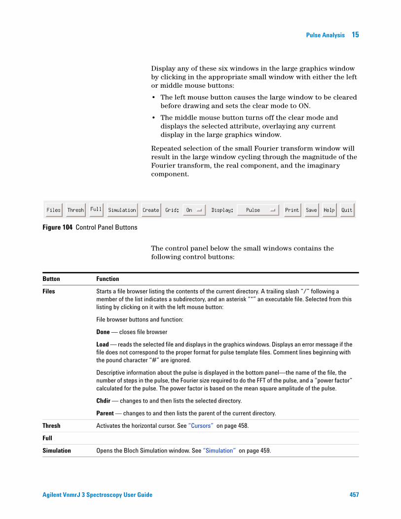
Pulse Analysis 15
Agilent VnmrJ 3 Spectroscopy User Gui
Display any of these six windows in the large graphics window by clicking in the appropriate small window with either the left or middle mouse buttons:
• The left mouse button causes the large window to be cleared before drawing and sets the clear mode to ON.
• The middle mouse button turns off the clear mode and displays the selected attribute, overlaying any current display in the large graphics window.
Repeated selection of the small Fourier transform window will result in the large window cycling through the magnitude of the Fourier transform, the real component, and the imaginary component.
Figure 104 Control Panel Buttons
The control panel below the small windows contains the following control buttons:
Button Function
Files Starts a file browser listing the contents of the current directory. A trailing slash “/” following a member of the list indicates a subdirectory, and an asterisk “*” an executable file. Selected from this listing by clicking on it with the left mouse button:
File browser buttons and function:
Done — closes file browser
Load — reads the selected file and displays in the graphics windows. Displays an error message if the file does not correspond to the proper format for pulse template files. Comment lines beginning with the pound character “#” are ignored.
Descriptive information about the pulse is displayed in the bottom panel—the name of the file, the number of steps in the pulse, the Fourier size required to do the FFT of the pulse, and a “power factor” calculated for the pulse. The power factor is based on the mean square amplitude of the pulse.
Chdir — changes to and then lists the selected directory.
Parent — changes to and then lists the parent of the current directory.
Thresh Activates the horizontal cursor. See “Cursors” on page 458.
Full
Simulation Opens the Bloch Simulation window. See “Simulation” on page 459.
de 457

15 Pulse Analysis
Cursors
Create Opens a drop-down menu of pulse types appears after a right mouse click the button. Hold down the mouse button and select one of the pulses in the menu. Release the mouse button to load the selected pulse type. See “Creating a pulse” on page 463.
Grid: ON/OFF menu Turns main window grid on or off.
Display: Pulse/Simulation menu
Displays the shaped pulse or, if the simulation has been run, a Block simulation of the response of the spins to the pulse
Print Click to print the main graphics window on a PostScript printer.
Save Saves the data currently displayed in the main graphics window to a file. 1 Click Save.
A filename entry field and a Done button are displayed.2 Type a filename.3 Click Save to write the file.
Repeat this as needed while in the save mode — display a different attribute in the main window; Type a new file name, and select Save.
4 Click Done to exit the save mode.
Help
Quit Close Pulsetool
Button Function
458
Interactive left, right, and horizontal cursors are available, and display a readout of position at the bottom of the large window when active. Click, using the left mouse button, anywhere on the large window to activate the left. Activate the right cursor by clicking the right mouse button anywhere to the left of the current single cursor. The right mouse button controls the position of the right cursor independently and the left mouse button moves the cursors in tandem.
The control panel button marked Full, when one cursor is active, changes to Expand, when both cursors are active. The display can be expanded to show the region between the two cursors.
NOTE The clear mode will always be set to ON after an Expand or Full operation.
Turn off a cursor by holding down the Control key and clicking the mouse button associated with the cursor. The right cursor is turned off by clicking the right mouse button in the large window, while simultaneously pressing the Control key.
Agilent VnmrJ 3 Spectroscopy User Guide

Pulse Analysis 15
Agilent VnmrJ 3 Spectroscopy User Gui
The horizontal cursor is activated with the Thresh button located in the control panel. When this cursor is active, it is controlled interactively with the middle mouse button. The interactive scale and reference functions that are normally controlled with the middle mouse are not available when the horizontal cursor is present. Select the Scale button in the control panel to turn off the horizontal cursor and reactivate the scale and reference functions (vertical scale and reference can be adjusted even with the horizontal cursor active by direct entry in the appropriate fields in the bottom panel).
Simulation
The simulation routine simulates the effects of an RF pulse by use of the classical model of nuclear spin evolution described by the Bloch equations. T1 and T2 relaxation effects are ignored, in which case, the evolution of a magnetization vector in the presence of an applied RF magnetic field can be evaluated by multiplication with a 3 by 3 rotation matrix. The simulation consists of repeated multiplication by such a matrix, whose elements are determined at each step by the values of amplitude and phase found in the pulse template file, and by user input values of initial magnetization, B1 field strength, pulse length, and resonance offset. The simulation is performed over one of three possible independent variables— resonance offset, B1 field strength, or time, and is determined by the Sweep cycle in the small button panel.
de 459

15 Pulse Analysis
Parameters
460
1 Click the Simulation button in the control panel to activate the Bloch Simulation window.
2 The Block Simulation window contains fields for entry of all required parameters (the pulse length is taken from the value in the bottom panel of the main window).
3 To change, type a value for any parameter by selecting it with the left mouse button and entering a value from the keyboard. Enter values for the parameters Mx, My, and Mz for the starting values of the magnetization components. Their vector sum must be less than or equal to 1.Click the Initialize button and select YES or NO. This feature works for Frequency and B1 sweep only, not Time.
Initialize cycle determines if the magnetization is re-initialized to the values of Mx, My, and Mz, or if the simulation uses the values at each point that were the result of the previous simulation. The effect of a series of pulses can be evaluated by loading the first pulse and performing the simulation with Initialize set to YES, loading subsequent pulse, setting Initialize to NO, and selecting Go after each pulse is loaded.
Agilent VnmrJ 3 Spectroscopy User Guide

Pulse Analysis 15
Agilent VnmrJ 3 Spectroscopy User Gui
4 Click the Sweep button and select Freq, B1, or Time for the sweep.
Freq
a Type a value in the B1max for B1 at the maximum pulse amplitude.
b Type a value in the Start Freq (KHz) field for the starting frequency.
c Type a value in the Stop Freq (KHz) field for the ending frequency.
B1
a Type a value in the Frequency (KHz) field for the how far the magnetization is off resonance.
b Type a value in the B1 Start (KHz) field for the starting B1 field.
c Type a value in the B1 Stop (KHz) field for the ending B1 field.
Time
The results are displayed in the form of a projected three-dimensional coordinate system, showing the path of the magnetization over the course of the pulse.
a Type a value in the B1max for B1 at the maximum pulse amplitude.
b Type a value in the Frequency (KHz) field to see how far the magnetization is off resonance.
5 Accept the default values or enter values for each of the following:
a Steps (not available if sweep is set to Time) — The number of steps used in the simulation
b Phase — Type the phase of the pulse
c Index — Counter that displays the current index. No entry is required for this parameter. Setting a value of 0 and clicking on the Steps button updates the parameters
d Step Inc.— Type the number of intermediate steps to be calculated each time the Step button is clicked
e Time — Type a non-zero integer value in this field to see the 3D display drawn in real-time
f Delay — Pre-pulse delay, in seconds. Normally not required. If defined, it disables the internal wave shifting according to the spin status.
de 461

15 Pulse Analysis
Performing a simulation
462
1 Click the Go button.
This action enables the simulation calculations to be done and then displays the results in the first five small graphics windows, replacing (but not destroying) the pulse information being displayed. The Fourier transform information remains unaffected, so that comparisons can be made between the information displayed and the exact simulation results.
All of the display functions described elsewhere is active as well, with the simulation data. Additionally, the original pulse data is still present in the background and can be swapped into view with the Display cycle found in the main control panel.
2 Click the Step button to view the course of the magnetization at intermediate stages through the pulse based on the value in the Steps Inc. field, starting at the current value of Index.
The intermediate result is then displayed in the normal fashion.
During a Go simulation, a small panel containing a Cancel button will pop into view. Use this to stop the simulation if necessary (there may be some delay between selecting the button and the end of the process).
Do not click Cancel more than once.
Clicking the Go button with Sweep: Set to Time displays the results in the form of a projected three-dimensional coordinate system, showing the path of the magnetization over the course of the pulse. This display is obtained by selecting the 3D button after first selecting the Go button. The left mouse button controls the viewing angle from within the canvas region delineated by the blue corner markers when the 3D display is active. This viewing angle is described by the two parameters phi (the amount of rotation about the Z-axis) and theta (the declination relative to the XY-plane). A “family” of trajectories can be displayed by first selecting any of the small canvases with the middle mouse button, then selecting the 3D button. Changing either the B1 field strength or the resonance offset followed by the Go button will result in display of the result without clearing the display. Select any of the small canvases with the left mouse button to reactivate the automatic clearing feature.
Agilent VnmrJ 3 Spectroscopy User Guide

Pulse Analysis 15
Creating a pulse
Agilent VnmrJ 3 Spectroscopy User Gui
The pulse creation routine currently offers the following pulse types:
A file containing the pulse template for any of these pulses can be created from scratch with this utility. Alternatively, pulses can be created for examination only, using the display capabilities of pulsetool. Each pulse is generated with user-definable parameters appropriate for the pulse in question.
1 Click the Create button and hold the right mouse button down.
2 Select a pulse type from the menu and release the mouse button.
Move the mouse arrow out of the menu area and release the button if none of the choices are acceptable.
A small window appears with a brief description of the characteristics of the pulse and a set of changeable attributes values when a pulse type is selected. The number of steps in the pulse is limited to powers of 2 and can be set by clicking on the left mouse button or by holding the right mouse button down and selecting the desired value from the resulting menu. All other attributes, which vary depending on the pulse type, can be altered from their default values by first selecting the appropriate field with the left mouse button, deleting with the Delete key, and typing in the desired value (clicking on the Return key is not required).
3 Select one of the following buttons at the bottom of the window:
• Preview — use the attributes as they appear on the screen to create a pulse that is loaded internally into pulsetool. All pulsetool features can then be used to examine and evaluate the new pulse. Any previous pulse information is deleted.
Square Hermite 90 Tan swept inversion
Sinc Hermite 180 Sin/cos 90
Gaussian Hyperbolic secant inversion
de 463

464
15 Pulse Analysis
• Execute — use the attributes as they appear on the screen to create a pulse and write it to a text file. The name of the file is taken from the file name field in the Create window and written into the current directory, listed in the Directory field in the bottom panel. If a file of the same name already exists, a prompt requests confirmation to overwrite the file. An error message appears if the program is unable to write to the named file. This is generally symptomatic of not having write permission in the current directory.
No new pulse types can be added to the list. User-created shaped pulse may be examined using the Files button.
Agilent VnmrJ 3 Spectroscopy User Guide

Agilent VnmrJ 3 SpectroscopyUser Guide
16Locator and File Browser
VJ Locator 466
Locator Statements 471
File Browser 474
This chapter provides information on the Locator and File Browser.
465Agilent Technologies

16 Locator and File Browser
VJ Locator
466
The VJ Locator, Figure 105, is a database browser that provides access to data sets, experiments, shim sets, commands, etc.
The Locator provides quick access to information on all or part of the disk environment. The administrator determines the scope of the Locator’s actions.
The Locator works similarly to a directory or file manager by using minimal information filtering and lists of information. Three lists are shown in the Locator when terms have a boolean relationship:
• Objects that meet all criteria
• Some of the boolean terms met
• Remaining objects
The construction of the underlying Locator statement determines which list is displayed.
Within each list, the Locator displays three attributes for each object. The displayed attributes may not be in the Locator statement. Any one of the attributes can be designated as the sort attribute. The objects in each list are sorted by the value each has for this attribute.
Figure 105 VJ Locator
Agilent VnmrJ 3 Spectroscopy User Guide

Locator and File Browser 16
Locator menu and controls
Agilent VnmrJ 3 Spectroscopy User Gui
The magnifying glass and the current Locator statement are at the top of the VJ Locator window, as shown in Figure 106.
Click the magnifying glass to open a menu of currently available Locator statements. This menu includes both statements provided by Agilent Technologies, Inc. and those customized and saved by the user.
Statements are Locator sentences in which a number of words or phrases are colored and underlined in a manner reminiscent of links in a web page. Each link hides a menu of choices, of which the currently displayed phrase is one. The choices available vary with the types of data currently known to the Locator.
Figure 106 Locator menus and controls
Navigation in the locator
A pair of arrows (statement navigation arrows) below the Locator statement enables searching forward and back through past Locator operations, applying each to the current Locator environment. Thus, a set of Locator statements can be rapidly applied in a changing environment.
de 467

16 Locator and File Browser
Attributes
468
The Attribute Header bar is below the icons. This bar enables selection of the attributes displayed and arrangement of the objects in each list in a number of ways.
The boundaries between the attribute labels are adjustable. Place the cursor on the boundary to adjust. When the adjust cursor appears, click and drag the boundary to its new position, and release.
Objects in the Locator are available for a number of actions. Currently, a single click selects an object. The selected object can then be dragged to another part of VnmrJ 3, in which case the action taken will depend on the type of object and where the object is dropped. Alternatively, double-clicking an object will cause the most likely action to occur. These actions are discussed below.
The value of an attribute might be longer than the width of the column in the Locator. When the mouse cursor rests on an attribute value, a tool tip appears for a period of time. The tool tip contains the full value of the attribute.
Attribute lists
The list of attributes in the drop-down lists is controlled by configuration files. There are three file names, for three different types of items in the locator:
• shuffler_param_list for 'vnmr data' and 'vnmr parameter' files
• study_param_list for 'study' items
• data protocol_param_list for 'protocol' items
Each of the above mentioned files can exist for each of the appmode types and for individual users. That is, appmode types of 'imaging', 'standard' (experimental liquids and solids), and 'walkup'. The attributes visible in the drop-down menu for each appmode type will be controlled by files in the appropriate directories. If a user does not have an individual file, the file in the appropriate appmode directories will be used. If there is no file in the imaging or walkup directories listed above, then the file in /vnmr/shuffler will be used. If users have their own individual files, the attributes listed must also be in the appmode directory file. That is, a user's files can limit the attributes shown, but cannot add to the list of attributes shown beyond the attributes in the system files.
Agilent VnmrJ 3 Spectroscopy User Guide

Locator and File Browser 16
Wildcards
Agilent VnmrJ 3 Spectroscopy User Gui
Wildcards can be used in attribute values, but not for the attribute name itself. For example, 'file*' to specify the autoboot 'filename' is not allowed. Selecting an attribute of 'filename', then editing the selection value to be 'p31*' to show all files whose names start with 'p31'. '?31*' shows all files starting with any single character followed by '31', followed by 0 or more characters. The leading '?' would allow upper or lower case 'P' as well as any other character. This does not apply to dates.
The following wildcards can be used:
• '*' or '%' can be used to match any number of characters
• '?' or '_' can be used to match any single character
Configuration files
Configuration files for the locator are contained in the following directories for the different appmode types:
Interface Directory
Standard (experimental) /vnmr/shuffler
Imaging /vnmr/imaging/shuffler
Walkup /vnmr/walkup/shuffler
Individual users $vnmruser/shuffler
Searches
Clicking on the magnifying glass icon with the left mouse button brings up a menu of searches. Selecting one changes the search sentence displayed at the top of the Locator. The results of the search are displayed in the list. Those items in the white part of the list satisfy the search sentence. Those in the gray part do not. For each item that is found by the search, three attributes are displayed. These correspond to the three columns in the list. Clicking on the attribute name at the top of the list with the left mouse button brings up a menu of attribute choices.
Dragging and dropping items from the locator
To select an item, click the item in the Locator list. The selected item can be dragged to the graphic area or the Parameter panel area for an appropriate action. For example, dragging a data set to the graphic area retrieves that data set into the current experiment workspace and can display the spectrum. Dragging
de 469

470
16 Locator and File Browser
a workspace to the graphic area selects that experiment workspace. Dragging an object causes the most likely action to occur.
An item can be dragged from the Locator and dropped into the holding pen. The item is then available for further selection, no matter which Locator statements are active. For example, use the Locator to inspect the available shim sets. Select the current best set and put this into the holding pen. This set of shims becomes available.
Dragging and dropping an item has an action appropriate to the context. Often the same effect can be obtained by double-clicking on an object. Some examples are:
• Drag a protocol experiment into the graphics canvas to load the experiment.
• Drag a FID from NMR data to retrieve the FID. The process macro can also be invoked so that the FID is transformed.
• Double-click a workspace to join that workspace. Dragging and dropping a workspace into the graphics area also joins the workspace (jexp).
• Double-click a parameter set to load that set in the current workspace, or drag and drop a parameter set.
• Double-click a shim set to load the shims. Dragging and dropping a shim set to the current shim buttons also loads the shims into acquisition.
• Drag either data or shims and drop them in the trash can (in the lower left portion of the hardware bar) to move the item to the trash can. Retrieve an object from the trash can by double-clicking on the trash can, selecting it, and then clicking on the Restore items button.
Editing file names from the locator
A new file added to the locator from within VnmrJ 3 appears in its appropriate spot in the Locator, and in green at the top of the locator window. If one of the columns in the Locator is filename, click the green file name to change it.
Change the file name, click Return or on another line to remove the old name from the Locator and add the new one. The Locator is redisplayed to show the new name.
Agilent VnmrJ 3 Spectroscopy User Guide

Locator and File Browser 16
Locator Statements
Agilent VnmrJ 3 Spectroscopy User Gui
Agilent supplies a number of Locator statements with VnmrJ 3. Add to or edit these statements in the following ways:
• Save the current Locator statement by clicking on Tools in the main menu, then Save Custom Locator Statement. Type a name for the statement in the Custom Locator Statement pop-up window.
• Click Tools, then Delete Custom Locator Statement to delete a Locator statement. A Custom Locator Statement Removal window appears. Select the statement from the list in the window, then click Delete to remove it or Cancel to exit the window without removing the statement.
• Sort Protocols Entries shows the known protocol experiments. Double-click the protocol to execute the associated macro.
Locator statements are defined in a file named locator_statements_default.xml.
This file can reside in the system appmode directories (see Configuration Files Configuration Files), but not in the user’s individual directories.
Editable fieldsClick the right mouse button on the blue and underlined items in the locator statements to show a menu of choices, and edit by clicking on them with the left mouse button. Left-clicking puts an editing cursor on the item. Place the cursor at the point to be edited and click the left mouse button. Edit the field, and then click Return to cause a new locator search using this edited value.
Sort workspaces
Sort all workspace in numeric order. Double-click a workspace to join the workspace.
Sort NMR Data
Entries show the known NMR data sets, but differ in the actual format of the statement as well as the initial set of attributes shown. The most comprehensive statement is the last one, by user defined attributes and date.
The generic statement is shown in Figure 107.
de 471

472
16 Locator and File Browser
There are two separate underlined choices in this statement: Std1D, on any date.
Click either of the underlined phrases to produce a drop-down menu of the choices in the selected position. The menus are environment sensitive and do not display choices that do not exist.
The logic of this statement is:
Show attributes A and B of type C with additional limitations.
First, the additional limitations phrases enable selection of the owner of the data. This selection is determined by the administrator at the time a directory is made available to the Locator.
Second, the additional limitations enable reordering by date. There are various dates associated with data, for example, the time started or the time saved. Specify these date fields in any of several ways, for example, since a certain date, by changing on any date to since.
Alter the date by using the left or right arrows to decrease or increase the date by one day with each click.
All other statements supplied are simpler than the generic one. Promote statements used frequently to the top of the menu by saving them again as your local variants.
Figure 107 Generic locator statement
Sort NMR parameter files
The statements in this category show the list of NMR parameter sets. One major category of parameter set is My Param Files. Select the statements Test Files and by user defined attributes to do other selective searches. The Locator statement changes after selecting a category.
Agilent VnmrJ 3 Spectroscopy User Guide

Locator and File Browser 16
Sort shimsets
Agilent VnmrJ 3 Spectroscopy User Gui
The statements in this category enable access to the saved shim sets. Note that the shim sets can be saved with a descriptive shim name provided when using the Save Shims button in the Shim panel.
Sort command macros
The generic statement in this category enables finding a VnmrJ 3 command or macro based on its attributes. The Locator enables reordering commands and macros by a number of attributes. Find the command to use and double-click to execute it.
de 473
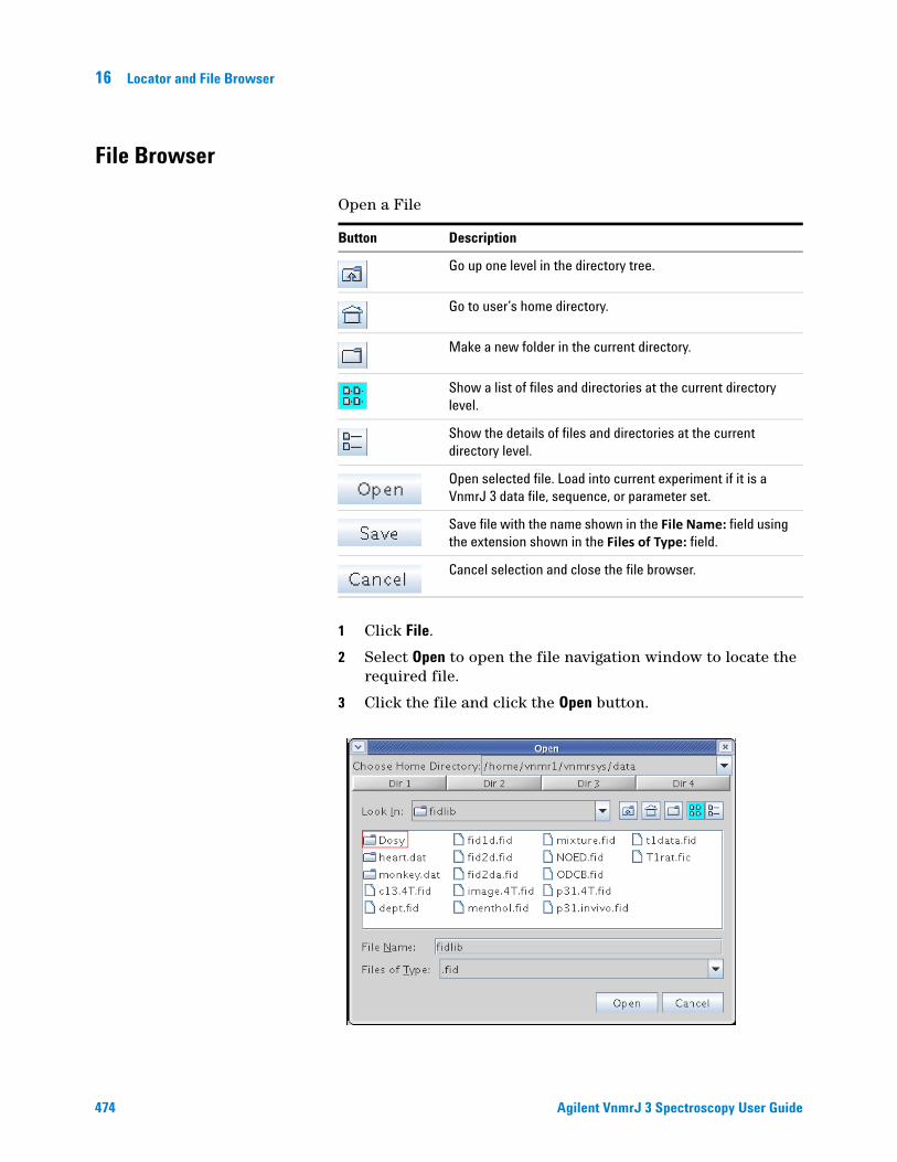
16 Locator and File Browser
File Browser
474
Open a File
1 Click File.
2 Select Open to open the file navigation window to locate the required file.
3 Click the file and click the Open button.
Button Description
Go up one level in the directory tree.
Go to user’s home directory.
Make a new folder in the current directory.
Show a list of files and directories at the current directory level.
Show the details of files and directories at the current directory level.
Open selected file. Load into current experiment if it is a VnmrJ 3 data file, sequence, or parameter set.
Save file with the name shown in the File Name: field using the extension shown in the Files of Type: field.
Cancel selection and close the file browser.
Agilent VnmrJ 3 Spectroscopy User Guide

Locator and File Browser 16
Agilent VnmrJ 3 Spectroscopy User Gui
Save a File
1 Click File.
2 Select Save as to open the file navigation window to locate the required directory.
3 Type a file name in the Save as field and click OK.
de 475

476
16 Locator and File Browser
Agilent VnmrJ 3 Spectroscopy User Guide

Agilent VnmrJ 3 SpectroscopyUser Guide
AStatus Codes
VT Setup 478
VT Startup 479
Temperature Array 480
Operating Considerations 481
VT Error Handling 483
VT Controller Safety Circuits 485
This chapter describes startup and operation of the optional variable-temperature (VT) unit. A VT unit is available for Agilent Technologies, Inc. NMR spectrometers to regulate the sample temperature. A thermocouple senses the temperature of the gas flowing over the sample; this temperature is then continuously displayed both in the software and on the optional remote status unit. The controller compares the user-requested value with the current probe temperature and changes the heater current accordingly. The VT controller then reports the temperature of the gas flow and status to the spectrometer through a serial port at the rear of the console.
477Agilent Technologies

A Status Codes
VT Setup
478
Use the System Settings window to configure the spectrometer for the VT accessory and to Type a VT (variable temperature) cutoff value. The VT cutoff (Edit / System settings / VT cutoff) determines which of the two gas streams in the system is supplied to the probe. (If the requested temperature is above the VT cutoff, it uses the high-temperature gas. If the requested temperature is below the VT cutoff value, it uses the low-temperature gas.)
1 Open the System Configuration window (Edit / System settings / System config) if the VT controller is off and it cannot be turned on.
2 Check that the VT Controller label is set to Present.
3 Open the System settings window (Edit / System settings) and type an appropriate value for VT cutoff and click OK.
Set the VT cutoff to a temperature near the ambient VT gas temperature (normally VT cutoff is correct and need not be changed). Based upon the value of VT cutoff compared to the typed temperature, the system selects either the high-temperature or low-temperature VT gas flow.
Agilent VnmrJ 3 Spectroscopy User Guide

Status Codes A
VT Startup
Agilent VnmrJ 3 Spectroscopy User Gui
The VT hardware must be installed and calibrated as described in the VT Accessory Installation manual. Starting up the VT unit takes the following steps:
1 Switch the VT unit on using the unit power switch (on the back of the spectrometer).
2 Reset the VT controller, if the system power has been off or the VT unit has been disconnected from the probe by pressing the POWER switch to turn the unit OFF, then press POWER again to turn it ON. The VT controller also can be reset with the Reset VT button on the Spin/Temp page in the Start tab.
CAUTION Use either dry nitrogen gas or dry air for VT and probe operation. A mixture of nitrogen gas and air can cause spikes in the baseline adjacent to the large peaks in the spectra. The use of air as the VT gas is not recommended for temperatures above 100°C. Such use will destructively oxidize the heater element and the thermocouple.
3 Use dry nitrogen gas if the requested temperature is over 100°C or below the dew point (or below 0° C, whichever is higher).
Otherwise, air may be used as the VT gas. If the requested temperature is below –40°C, dry nitrogen gas is recommended for cooling the bearing, spinner, and decoupler. This prevents moisture condensation in the probe and spinner housing.
The source of heating or cooling gas is not automatically selected. To use nitrogen, attach a nitrogen gas source to the VT system. The same is true when using air. The VT system only selects the routing of the gas flow.
4 Use the flow control meter on the magnet leg to adjust the flow to about 10 LPM (as shown on the flow gauge).
5 Place a sample that can be handled at ambient temperature and be placed in the probe, NMR lock obtained, and field homogeneity adjusted. Samples that cannot be handled at ambient temperature should wait until the system reaches the requested temperature.
de 479

A Status Codes
Temperature Array
480
If an array of sample temperatures is to be used, set a pre-acquisition delay (pad) that allows sufficient time for the sample to equilibrate after a temperature change. The system will then wait pad between each temperature before starting data acquisition. Delays of several minutes are optimum because the sample will take longer to equilibrate than it takes the VT controller to stabilize the heating/cooling gas at the setpoint.
1 Open the Acquire / Acquisition page, and click the Arrays button – or select Acquisition / Parameter arrays.
This opens the Array Parameter window.
2 Click New Array and type temp in the Param Name column.
3 Specify Array Size, First Value, Increment, and Last Value.
4 Click Close.
5 Set the pre-acquisition delay in the Acquire / Flags page.
6 Delay __ sec before starting (for VT etc.)
Agilent VnmrJ 3 Spectroscopy User Guide

Status Codes A
Operating Considerations
Agilent VnmrJ 3 Spectroscopy User Gui
Use the following recommendations to help achieve better VT performance.
• The spectrometer system was designed and tested with a VT gas flow rate of about 10 – 15 LPM. Sizable deviation from this rate can result in significant inaccuracy in temperature calibration and reduce the attainable temperature limits.
• Initial cool-down of the exchanger and transfer tubing after the coolant is added increases the initial time required to reach regulation (about 5 to 10 minutes for –40°C with liquid nitrogen). This may be longer than the vtwait parameter (this is the longest time the su command will wait for the temperature to equilibrate).
• Below –40°, use dry nitrogen gas for the spinner and bearing air supply to avoid moisture and frost buildup on the spinner housing and turbine. Should this happen, the sample spinning can become erratic or stop altogether.
• Every sample has some amount of temperature gradient along the vertical axis. Minimize the gradient by not filling the sample tube more than about 25 to 32 mm (1 to 1.25 in.) for VT samples, by inserting a vortex plug or glass wool plug in the tube just above the sample solution, and by placing the liquid column at the probe-coil cType lines. The plug reduces refluxing of the solvent in the upper portion of the tube. Any mass movement, such as refluxing or convection, can seriously degrade resolution and lock stability.
• Above 100°C, use dry nitrogen gas to reduce oxidation of the heater and thermocouple.
• High-power decoupling adds heat to the sample. (It does so internally – within the sample – meaning that the temperature readout does not reflect this heating.) The increase in temperature depends on the dielectric of the solution and the power level. Under these conditions, the temperature accuracy can be affected. If necessary, reduce decoupler power and use a more efficient decoupling mode.
de 481

482
A Status Codes
• Overnight or long-term unattended VT operation at low temperatures is hampered by the fact that the usual coolant, liquid nitrogen, provides only about 1 to 2 hours of operation on a single fill of the coolant bucket. Some other coolant that lasts longer can be used if the operating temperature does not require the low temperature of liquid nitrogen. A common alternative is a mixture of dry ice and isopropyl alcohol (or ethylene glycol). (Do not use acetone – it will dissolve the bucket!) Another option is to cool the fluid indirectly by a refrigerating device such as isopropyl alcohol or ethylene glycol cooled. Do not use aromatic, ketone, or chlorinated solvents (including acetone) in the coolant bucket, because these solvents will dissolve the standard polystyrene bucket.
• On older spectrometers, the ability of the VT unit to achieve temperature stability is affected by the stability of the room temperature. For best results, the room temperature should be made as stable as possible.
• An optional setup to help stabilize the VT gas supply is to run the VT gas through a heat-exchanger coil in a water bath at a regulated temperature. For best results, use an ice bath to cool down the VT gas to between 5°C and 10°C, and keep the flow as stable as possible for experiments below 40°C. Generally, the VT gas supply temperature should be a minimum of 10°C below the set temperature of the VT controller to get the best performance of the VT controller and heater in the probe.
• A temperature calibration curve must be made for each probe if you want an exact determination of sample temperature. All data, such as gas flow rates, must be noted. Samples of ethylene glycol are used for high-temperature calibration, and samples of methanol are used for low-temperature calibration.
a Obtain a spectrum after bringing the sample to the desired temperature and allowing sufficient time for equilibration. Note that these samples have no lock solvent, and usually require additional shimming due to their short sample length (to reduce temperature gradients).
b Display two cursors and align them on the two resonances in the spectrum.
c Type tempcal('e') if the sample is ethylene glycol. If the sample is methanol, type tempcal('m').
d The temperature is calculated and displayed based on the difference in frequency between the cursors.
Agilent VnmrJ 3 Spectroscopy User Guide

Status Codes A
VT Error Handling
Agilent VnmrJ 3 Spectroscopy User Gui
Select how VT errors are handled in the Spin/Temp page under the Start folder.
Interlock selections Wait setting
(Start folder, Spin/Temp page) (Acquire folder, Flags page)
Abort after temperature error The VT regulation light is monitored during the course of the experiment, and if it starts to flash (regulation lost), the current data acquisition is stopped. The acquisition does not resume automatically if regulation is regained. With Abort selected, a maximum limit is imposed on the time that the system waits for regulation to be established (vtwait, the "wait before testing setting"). This time is independent of the delay setting (pad). If regulation is not established after the wait time (vtwait, normally set to 300 seconds), the system displays the message VT FAILURE and does not proceed with the experiment. If the regulation problem is later corrected, the experiment can be resumed.
Warn after temperature error The VT regulation light is monitored during the course of the experiment, and if it starts to flash (regulation lost), a warning is generated, but acquisition is not stopped.
Ignore temperature error The temperature interlock feature is turned off.
The temperature interlock selections (Abort, Warn, or Ignore) and VT wait time (Acquire folder, Flag page) check VT operation and stop the experiment if temperature regulation is lost.
The lost regulation causes error processing to occur for both the Abort and Warn selections, thus providing a user-selectable mechanism to respond to VT failure.
The interlock operation does not apply when VT regulation is temporarily lost as a result of a programmed temperature change in an experiment where temperature is an array. The VT gas flow has a sensor and an interlock on VNMRS and 400MR consoles. Additionally, the heater is protected if gas flow stops by an internal temperature limit sensor that turns off the heater current before the element overheats. Any experiment in progress is stopped if Abort is selected because a loss of gas flow will result in a loss of regulation. Only the sample is left unprotected if VT gas stops.
de 483

A Status Codes
CAUTION Do not run unattended a sealed sample of highly volatile materials that must be kept cold to avoid excessive pressure buildup. The undetected loss of VT gas or exchanger coolant could result in the rupture of the sample tube and damage to the probe components.
484 Agilent VnmrJ 3 Spectroscopy User Guide

Status Codes A
VT Controller Safety Circuits
Agilent VnmrJ 3 Spectroscopy User Gui
The VT controller includes safety circuits to avoid damage to the heating element and probe. The following error conditions produce an error code:
• Open circuit in the thermocouple circuit
• Open circuit, short circuit, or over-temperature at safety senso
• Short circuit or software/microprocessor failure at the output transistor
Over-temperature at the safety sensor initially turns off the heater. If this method fails to correct the condition within 5 seconds, either the gas flow has been interrupted or an output transistor failure has occurred, whereupon a protective relay operates, isolating the heater from the control electronics. Failure of any of the sensors also results in this relay operating.
Once the protective relay has operated, the output will remain off. A power-down and power-up cycle of the VT controller is required to release the relay.
The over-temperature circuit can be inadvertently tripped if the VT is started at a below ambient temperature and the temperature is increased greater than 70°C. If the circuit is tripped, reset it by turning the VT off and on, then change to the desired temperature in 50°C steps.
Excessive heat requirements that cause the current to remain near the maximum can also trip the second circuit. Therefore, when using liquid nitrogen for cooling and when operating above 0°C, reduce the gas flow rate to between 8 and 9 LPM. Reset will also occur if the VT cable is removed from the probe while the VT is on.
See the VT Accessory Installation manual for system failure analysis.
de 485

486
A Status Codes
Agilent VnmrJ 3 Spectroscopy User Guide

Agilent VnmrJ 3 SpectroscopyUser Guide
BShimming Basics
Shim Interactions 489
Autoshim Information 495
Homogeneity Commands and Parameter 503
The room-temperature shims coils, which are commonly referred to as just "the shims", are a set of coils inside the magnet's room-temperature bore that induce small changes in the shape of the magnetic field. Each shim produces a specific change in the magnetic field that can be easily shown. The approximate shapes of the axial gradients (spinning shims) are shown in Figure 108 to provide a visual reference for the interactions of the shims.
Understanding the effect of various shims on the symmetry of the resonance is important in simplifying the shimming process.
Figure 108 Approximate shape of axial gradients
487Agilent Technologies

488
B Shimming Basics
The following two points must be considered:
• The effect of a given shim on the spectral lineshape
• How the shims interact with each other
Understanding how the shims interact is critical to simplifying the task of shimming. Pure shim gradients produce a very specific and predictable effect on the magnetic field and, to a lesser extent, on the resonance lineshape.
Agilent VnmrJ 3 Spectroscopy User Guide

Shimming Basics B
Shim Interactions
Agilent VnmrJ 3 Spectroscopy User Gui
The following sections show theoretically predicted changes in lineshape caused by changes in shim DAC values. Shim sets with pure shims, such as the Agilent Ultra•nmr shims, follow the theoretically predicted response very closely. Other shim systems, with more interactions between shims, produce different results.
Theoretically perfect lineshape and effect of Z1 shim
Figure 109 shows a theoretically perfect lineshape (at left) produced in a perfectly homogeneous field (at right). The magnetic field shape appears as a flat line, indicating that the magnetic field does not change across the length of the sample.
Figure 110 shows how changing the linear shim Z1 affects both the lineshape (left) and the magnetic field (right).
Figure 109 Theoretically perfect lineshape
Figure 110 Effects of linear shim Z1
de 489
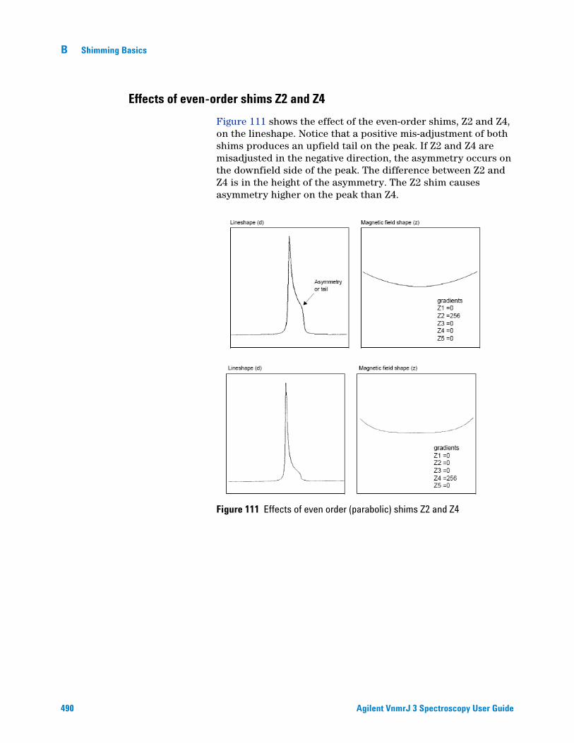
B Shimming Basics
Effects of even-order shims Z2 and Z4
490
Figure 111 shows the effect of the even-order shims, Z2 and Z4, on the lineshape. Notice that a positive mis-adjustment of both shims produces an upfield tail on the peak. If Z2 and Z4 are misadjusted in the negative direction, the asymmetry occurs on the downfield side of the peak. The difference between Z2 and Z4 is in the height of the asymmetry. The Z2 shim causes asymmetry higher on the peak than Z4.
Figure 111 Effects of even order (parabolic) shims Z2 and Z4
Agilent VnmrJ 3 Spectroscopy User Guide

Shimming Basics B
Effects of odd-order shims Z3 and Z5
Agilent VnmrJ 3 Spectroscopy User Gui
Figure 112 shows the effects of the odd-order shims Z3 and Z5 on the lineshape. The odd-order shims cause broadening of the peak and therefore affect resolution. The Z5 shim is unavailable on systems with 13-channel shim sets (shimset=1).
Figure 112 Effect of odd order (non-linear) shims Z3 and Z5
de 491

B Shimming Basics
Effects of improperly adjusted shims
492
Figure 113 shows two examples of the effects when more than one shim is improperly adjusted. This is the typical case with real samples. The complex lineshapes make simple visual analysis difficult. A procedure for correcting the shims that can be used as a guide when adjusting shims is provided later in this section.
Figure 113 Effects of misadjusted shims
Agilent VnmrJ 3 Spectroscopy User Guide

Shimming Basics B
Effects of Non-Spin Shims
Agilent VnmrJ 3 Spectroscopy User Gui
Figure 114 shows the effect of the non-spin shims on the spectrum (note that Z3X and Z3Y are not available on 13- or 14-channel shim systems). If set wrong, the first-order non-spin shims (X, Y, ZX, and ZY) can cause first-order spinning sidebands. XY and X2–Y2 can cause second-order spinning sidebands. High-order non-spin shims can cause a broad peak base.
Figure 114 Effects of nonspin shims
de 493

B Shimming Basics
Summary of shim interactions
494
Table 45 lists some lineshape effects associated with shims. Note that the 13-channel shim systems (shimset=1) do not have Z5, Z3X, ZXY, etc., and that the 14-channel shim systems (shimset=10) have Z5 but do not have Z3X, ZXY, etc.
Typical interactions for axial shims:
• Z1 and all other axial shims, to some extent
• Z2 and Z1
• Z3 and Z1
• Z4 and Z2 (with large delta Z4s: Z4 and Z3)
• Z5 and both Z3 and Z1 (Z5 not available on 13-channel shim systems)
Table 45 Lineshape effects and their associated shims
Lineshape effect Shims
Split peak Z4 and Z1
Asymmetry greater than half-way up Z2
Asymmetric foot Z4
Symmetric feet and or low broad base Z5
Symmetrically broad base Z3
Spinning sidebands Low-order radials X1, Y1
Symmetric broad base High-order radials X3, Y3, etc
Agilent VnmrJ 3 Spectroscopy User Guide

Shimming Basics B
Autoshim Information
Agilent VnmrJ 3 Spectroscopy User Gui
Gradient autoshimming is the preferred method for shimming. There are also other (slower) methods that use the lock signal. These methods are Hardware and Background Autoshim.
Hardware autoshim
Hardware autoshim methods vary according to the system that is involved. They are used primarily to maintain a well-shimmed homogeneity over long runs.
The hdwshim parameter enables the commands su, go, ga, or au to turn on and off “hardware” autoshimming, which is done using a software emulation of hardware autoshim. Shimming is active only while a pulse sequence is executing:
• hdwshim='y': shimming is active only during the first delay of the pulse sequence
• hdwshim='p': shimming is active only during the first presaturation pulse, defined as a change in power level followed by a pulse (for example, presat.c)
Shimming during subsequent delays or presaturation pulses can be activated by using the hdwshiminit() statement before the delay or presaturation pulse. Shimming uses the z1 shim by default.
If the parameter hdwshimlist is created, shimming will be done on only the specified list of shims. Only the following shims are allowed:
z1, z1c, z2, z2c, x1, y1
Shimming is done in the order of z1, z1c, z2, z2c, x1, y1, regardless of the order in which the shims are used in hdwshimlist, and is performed on each shim in intervals of 20 seconds. The fine shims (z1, z2, x1, and y1) are recommended for routine use.
de 495

B Shimming Basics
Using the input window
496
• Type hdwshim='y' su.
Hardware shimming starts at the next acquisition – a during the first delay – and stops when acquisition is complete.
• Type hdwshim='p' su.
Hardware shimming starts at the next acquisition – during the first presaturation pulse – and stops when acquisition is complete.
• Type hdwshim='n' su to turn off hardware shimming.
Method autoshim
Method Autoshim is controlled by the parameter method and the command shim. This is an Autoshim method that provides no interaction with the operator. The shimmethod (method) that should be used during routine sample changes depends upon the level of homogeneity required, the change in sample height between samples, and the maximum time desired for shimming.
• For samples that are either long or all of identical height, and with average homogeneity needs: a simple z1z2 shimming is usually sufficient (method='z1z2').
• For samples where the sample height might vary: the method allzs has been found to be the most reliable, at the expense of greater time spent in shimming. This method shims first Z1, Z2, and Z4, then Z1, Z2, and Z3, and finally Z1 and Z2.
Using the input window
Type method=file shim, where file is the name of a file in the directory shimmethods (for example, method='z1z2' shim).
Two shimmethods directories can exist. A user can have a private copy of shimmethods in a personal shimmethods directory. A system-wide set of shim methods is also located in the /vnmr/shimmethods directory. The user’s private library is searched first for a given method. If the method is not found in the user’s directory, then the directory /vnmr/shimmethods is searched.
Shimming methods can be used in succession or strung together. For example, Typing method='z1z2' shim shim would cause the method in the file z1z2 (Z1, Z2 shimming) to be used, as indicated by its code, twice in succession, and Typing method='z1z2' shim method='nsm' shim shim shim would cause the first method to be used once and the second method three times.
Agilent VnmrJ 3 Spectroscopy User Guide

Shimming Basics B
Shimming criteria for method autoshim
Agilent VnmrJ 3 Spectroscopy User Gui
Two aspects of Autoshim must in some way be specified by the user. One is the resolution of the starting point—good or bad? If good, only small changes need to be made to the shim settings to find the optimum, if bad, larger changes are necessary. The second is how good must the final resolution be? Clearly, the better the desired resolution, the smaller the steps that Autoshim must take as it approaches the maximum, in order to find the absolute maximum to within a specified degree.
As shown in Table 46, there are five criterion values: B (bad), L (loose), M (medium), T (tight), and E (excellent). (The lower-case letters are used when Typing criterion values into a shim method, discussed below).
A full criterion consists of two letters, for example, L > M indicates a loose starting criterion (the shims are expected to be far from their desired values) and a medium ending criterion (end with “normal” shim quality). Tight and excellent are only used for extremely high resolution, where the beginning resolution is very nearly that desired.
Specify the starting and ending points as L > M if poor resolution is suspected and improvement is needed without spending the time necessary to get excellent resolution.
The duration of automatic shimming is a function of these criteria. Therefore, try to make an informed choice with respect to the resolution needed and, in particular, for FID shimming, the choice of acquisition time as specified in the parameter table. An acquisition time of 2 seconds gives a limiting digital resolution of 0.5 Hz, a resolution that would be inconsistent with shimming to a tight criterion. In the interactive shimming mode using acqi, only the most important criteria are accessible to the user: L > M, M > M, M > T, and T > T (B and E are inaccessible).
Table 46 Permissible shimming criterion values
Criterion Meaning Recommended Usage
B or b Bad No decent starting shim values available
L or l Loose Extreme change in sample height
M or m Medium Typical sample change
T or t Tight Resolution desired above average
E or e Excellent Resolution desired less than 0.2 Hz
de 497

498
B Shimming Basics
The starting criterion should never affect the final result, only the time taken to get the result. If the starting criterion is specified as T, for example, and the optimum shim is far off, this shim will eventually be found. The search may take longer than if a starting criterion of L had been specified.
Shim methods for autoshim
Table 47 lists standard two-character codes for shim gradient combinations.
Table 47 Codes for standard shim gradient combinations
Standard code Gradients Hexadecimal code
z1 Z1C 0000008
z2 Z2C 0000020
z3 Z3 0000040
z4 Z4 0000080
z5 Z5 0000100
zq Z1C,Z2C 0000028
zt Z1C,Z2,Z3 0000068
zb Z1C,Z2C,Z4 00000A8
za Z1C,Z2C,Z3,Z4,Z5 00001E8
ze Z2C,Z4 00000A0
zo Z1C,Z3,Z5 0000148
zc Z1C,Z2C,Z5 0000128
zm User-selected gradients User-Typeed
tx X,Z1 0010004
ty Y,Z1 0020004
t1 X,Y,Z1 0030004
t2 X,Y,XY,YZ,X2,Y2,Z1 03B0004
tz X,Y,XZ,YZ,Z1 0270004
tt X,Y,XZ,XY,X2Y2,YZ,Z1 03F0004
t3 X,Y,XZ2,YZ2,Z1 5030004
t4 X,XZ,X3,XZ2,Z1 4450004
t5 Y,YZ,Y3,YZ2,Z1 1A20004
t6 XY,X2Y2,ZX2Y2,ZXY,Z1 A180004
Agilent VnmrJ 3 Spectroscopy User Guide

Shimming Basics B
Agilent VnmrJ 3 Spectroscopy User Gui
A shim method consists of a text string contained in a file within the shimmethods directory of either the VnmrJ 3 system or a user. That text string is interpreted as a series of instructions describing the shimming method. Commands in elements include:
• Turn on and off the spinner
• Set maximum shim time per element
• Set the delay between lock level samplings
• Specify the gradients to be shimmed and the criterion used for shimming
A complete method consists of one or more elements, separated by commas and terminated with a semicolon (for example, f,ry,t600,szq:cmm;). The element setting for specific gradient or gradients to be shimmed has the syntax sxx:cyz, where s identifies the shim part of the form, xx is a two-character code for a specific shim gradient or gradient combination, c identifies the criterion part of the form, y is the starting criterion, and z is the desired ending criterion.
See the description of the shimset parameter in the VnmrJ 3 Command and Parameter Reference for a list of shims in each type of shim set.
The following examples show the meaning of a few standard shim methods:
• szq:cmm; means set shims Z1C and Z2C with a medium to medium criterion.
• sza:clm; means shim all Z gradients with a loose to medium criterion.
• szt:clm,szb:clm,szq:cmm; means shim Z1C, Z2, and Z3 with a loose to medium criterion, then shim Z1C, Z2C, and Z4 with a loose to medium criterion, and lastly shim Z1C and Z2C with a medium to medium criterion.
t7 X,Y,XZ,XY,X2Y2,YZ,X3,Y3,YZ2,ZX2Y2,XZ2,ZXY,Z1
FFF0004
ta X,Y,XZ,XY,X2Y2,YZ,YZ2,XZ2,1
53F0004
tm User-selected gradients User-typed
Table 47 Codes for standard shim gradient combinations (continued)
Standard code Gradients Hexadecimal code
de 499

B Shimming Basics
User-defined shim methods for autoshim
500
The shim methods supplied with the system are based on a series of “standard” coil groupings. Automatic shimming operation using other groups of shims than are provided is supported by creating user-defined shim methods. For example, shimming Z1, Z3, and Z4 while holding Z2 fixed.
Certain combinations of shim coils can be selected by constructing a 7-digit hexadecimal (base 16) number based upon the following shim coil chart:
To construct a method for this example, first notice in the diagram that Z1 is represented by a 4 in the first digit (on the far right) and that Z4 and Z3 are represented by a 8 and 4, respectively, in the second digit, which gives a total of 12 (or C in hexadecimal notation). The rest of the digits are 0 because no other shimming is desired. Thus, the seven-digit hexadecimal number representing Z1, Z3, and Z4 is 00000C4. This number is then prefixed by zm or tm (the two are equivalent) making szm00000C4 the method desired.
Some examples of user-selected methods:
• stm0A30004:clm; means shim Z1, X1, Y1, YZ, Y3 with loose to medium criterion.
The hexadecimal code for each standard coil grouping is listed in the third column of Table 47 on page 498.
The following codes enable control of other aspects of automatic shimming:
• l sets shimming on the lock instead of the FID (default).
• f sets shimming on the FID instead of the lock.
• f:0,90 sets shimming on the FID with limits for the FID evaluation range. Full range is 0 to 100 percent of the duration of the FID. Sensitivity to higher-order spinning gradients is increased with a start of 0 and a finish limit of about 5 or 10, which weights the evaluation to the front of the FID.
• ry (rotation yes) turns the spinner on.
ZX
YX
Z2
ZX
2Y
2Y
Z2
Y3
X3
YZ
X2Y
2
XY
XZ
Y1
X1
— — — — — — — Z5
Z4
Z3
Z2C
Z2
Z1C
Z1
Z0
—
8 4 2 1 8 4 2 1 8 4 2 1 8 4 2 1 8 4 2 1 8 4 2 18 4 2 1
Agilent VnmrJ 3 Spectroscopy User Guide

Shimming Basics B
Agilent VnmrJ 3 Spectroscopy User Gui
• rn (rotation no) turns the spinner off.
• dx sets a delay x hundredths of seconds between lock samplings. Variations in lock solvent T1 and T2.relaxation times affect the ability of automatic shimming to attain good resolution in reasonable times. If too short, automatic shimming will not be performed properly. If too long, the shimming will become unacceptable in duration. dx allows setting an appropriate delay and can be used one or more times within a text string. If no entry is made using dx, the system automatically measures the lock response and sets a delay accordingly.
• tx sets the maximum shimming time to x seconds. Once tx is set, it governs all future shim elements within a method string, just as dx governs the lock sampling interval for all shim elements until changed. If tx is not set, the shimming will proceed based on internal program criteria.
• q recalls an algorithm’s internal parameters so that shimming starts quickly. q is a background autoshim that keeps the magnetic field at an optimum during experiments of long duration. Shimming is performed at the time wshim instructs. Only the portion of the shim methods following the letter q is executed after the experiment’s first increment. Any shim method may follow q. However, the sz1 (Z1 only) and szq (Z1, Z2) are the most effective. Multiple shim methods may follow q, but time effectiveness is reduced.
Methods may be typed into the shimmethods file using a text editor such as vi. The macros newshm and stdshm provide an interactive method of defining shim methods. Note that unlike normal text files, which have unrestricted size, the maximum text file size for a shim method is 128 characters.
The following examples show complete user-defined shim methods:
• szq:cmm,rn,stz:cmm,ry,szq:cmm; means shim Z1C, Z2C with medium to medium criterion, turn off spinner, shim X, Y, XZ, YZ, Z1 with medium to medium criterion, turn on spinner, and then shim Z1C, Z2C again with medium to medium criterion throughout.
• d50, szq: cmm, d150, sza: cmm; means to sample every 0.5 seconds while shimming Z1C, Z2C, and then to sample every 1.5 seconds.
• t60,szq:cmm,t240,sza:cmm; means shim Z1C, Z2C for 60 seconds maximum, then shim all Z gradients for a maximum of 4 minutes. Use medium to medium criterion throughout.
de 501

502
B Shimming Basics
• f,ry,t600,szq:cmm; means turn on spinner and FID shim Z1C, Z2C with medium to medium criterion for 10 minutes maximum (not available on GEMINI 2000).
• t60,sza:cmm,q,t30,sz1:cmm; (with wshim='f20') means initially shim on all Z gradients for 60 seconds, then shim Z1. After every 20 FIDs, shim Z1 for 30 seconds.
• sza:cmm,q,t30,szq:cmm; (with wshim='f10') means initially shim on all Z gradients (with no time out) and then perform a Z1, Z2 shim for 60 seconds every 10 FIDs.
Agilent VnmrJ 3 Spectroscopy User Guide

Shimming Basics B
Homogeneity Commands and Parameter
Command Description
dgs Display shim and automation parameter group
diffshims(shimfile1,shimfile2) Compare two sets of shims (VNMR)
diffshims shimfile1 shimfile2 Compare two sets of shims (Linux)
dshim<(file)>,dshim('method'|'help') Display a shim “method” string
gmapshim<('files'|'mapname'|'quit')> Start gradient autoshimming
gmapsys Setup gradient shimming
newshm Interactively create shim method
readallshims Read all shims from hardware
readhw(par1,par2,...)<:var1,var2,...> Read acquisition hardware values
rts(file)<:status> Retrieve shim coil settings
setallshims Set all shims into hardware
sethw* Set acquisition hardware values (shim-related)
shim Submit an Autoshim experiment
stdshm Interactively create a shim method
Svs(file)<:status> Save shim coil settings
*sethw(<'wait'|'nowait',>par1,val1<,par2,val2,...)
Parameters
gmap_findtof {'n','y'} Find tof before start of gradient shimming
gmap_z1z4 {'n','y'} Gradient shim z1-z4, then higher-order shims
hdwshim {'n','y','p'} Hardware shimming (if available)
hdwshimlist {'z1','z1z2x1y1'...} List of shims for hardware shimming
load {'n','y'} Load status of displayed shims
method {file in shimmethods} Autoshim method
shimset {1,2,3,...14} Type of shim set
shimspath {absolute path} Path to user’s shims directory
wshim {'n','e','s','g','f','f#'} Conditions when to shim
x1, y1, z1,... Shim gradients X1, Y1, Z1...
z0 {-2048 to 2047, -32768 to 32767} Z0 field position
Agilent VnmrJ 3 Spectroscopy User Guide 503

504
B Shimming Basics
Agilent VnmrJ 3 Spectroscopy User Guide

Agilent VnmrJ 3 SpectroscopyUser Guide
CLiquids Spectra
Ethylindanone 506
Azithromycin 509
Clindamycin 510
Paclitaxel 511
Sucrose 512
Vitamin B12 513
3-Acetyl-2-Fluoropyrimidine 514
Following is a short description of the liquids spectra found in the /vnmr/fidlib directory.
505Agilent Technologies

C Liquids Spectra
Ethylindanone
506
Sample Ethylindanone (M = 160) 10 mg in CDCl3Spectrometer 400-MR + OneNMR probeDirectory /vnmr/fidlib/EthylindanoneMolecule /vnmr/mollib/Ethylindanone.mol
Ethylindanone_PROTON_01.fid 4 s 1D 1H (1 scan)
Ethylindanone_CARBON_01.fid 9 min 45 s 1D 13C (256 scans)
Ethylindanone_gCOSY_01.fid 3 min 10 s 2D gradient COSY
Ethylindanone_COSY_01.fid 5 min 41 s 2D COSY
Ethylindanone_gDQCOSY_01.fid 8 min 27 s 2D gradient double quantum COSY
Ethylindanone_DQCOSY_01.fid 31 min 49 s 2D double quantum COSY
Ethylindanone_TOCSY_01.fid 17 min 21 s 2D TOCSY (Total Correlation SpectroscopY)
Ethylindanone_zTOCSY_01.fid 18 min 23 s 2D z-TOCSY (Total Correlation SpectroscopY along z-axis)
Ethylindanone_NOESY_01.fid 47 min 18 s 2D NOESY (200 ms mixing)
Ethylindanone_ROESY_01.fid 47 min 17 s 2D ROESY (200 ms spinlock)
Ethylindanone_ROESYAD_01.fid 47 min 28 s 2D ROESY with adiabatic spinlock (200 ms)
Ethylindanone_HOMO2DJ_01.fid 6 min 24 s 2D HOMO2DJ (J-resolved)
Ethylindanone_HSQCAD_01.fid 8 min 15 s 2D 1H-13C HSQC with adiabatic pulses
Ethylindanone_gHSQCAD_01.fid 8 min 18 s 2D 1H-13C gradient HSQC with adiabatic pulses
Ethylindanone_HSQC_01.fid 8 min 15 s 2D 1H-13C HSQC
Ethylindanone_gHSQC_01.fid 8 min 15 s 2D 1H-13C gradient HSQC
Ethylindanone_HMQC_01.fid 8 min 8 s 2D 1H-13C HMQC
Ethylindanone_gHMQC_01.fid 8 min 12 s 2D 1H-13C gradient HMQC
Ethylindanone_ASAPHMQC_01.fid 1 min 23 s 2D 1H-13C ASAP-HMQC (fast 2D HMQC)
Ethylindanone_gHMBCAD_01.fid 1 h 6 min 2D 1H-13C gradient HMBC with adiabatic pulses
Ethylindanone_gHMBC_01.fid 1 h 6 min 2D 1H-13C gradient HMBC
Ethylindanone_gH2BCAD_01.fid 43 min 52 s 2D 1H-13C gradient H2BC (2-bond specific long-range correlation) with adiabatic pulses
Ethylindanone_gH2BC_01.fid 45 min 25 s 2D 1H-13C gradient H2BC (2-bond specific long-range correlation)
Ethylindanone_CIGAR_01.fid 1 h 8 min 2D 1H-13C CIGAR (HMBC-type)
Ethylindanone_CIGARAD_01.fid 1 h 8 min 2D 1H-13C CIGAR with adiabatic pulses (HMBC-type)
Ethylindanone_HMBC_01.fid 1 h 6 min 2D 1H-13C HMBC
Ethylindanone_gHMBCmeAD_01.fid 2 h 13 min 2D 1H-13C gradient HMBC with adiabatic pulses (multiple-bond correlation with multiplicity editing,go to Processs -> Default to transform subspectra)
Agilent VnmrJ 3 Spectroscopy User Guide

Liquids Spectra C
Ethylindanone_HSQCADTOXY_01.fid 22 min 21 s 2D 1H-13C HSQC-TOCSY with adiabatic pulses (80 ms spinlock)
Ethylindanone_gHSQCADTOXY_01.fid 1 h 27 min 2D 1H-13C gradient HSQC-TOCSY with adiabatic pulses (80 ms spinlock)
Ethylindanone_HSQCTOXY_01.fid 22 min 23 s 2D 1H-13C HSQC-TOCSY (80 ms spinlock, direct correlations inverted)
Ethylindanone_gHSQCTOXY_01.fid 1 h 27 min 2D 1H-13C gradient HSQC-TOCSY (80 ms spinlock, direct correlations inverted)
Ethylindanone_HMQCTOXY_01.fid 22 min 14 s 2D 1H-13C HMQC-TOCSY (80 ms spinlock, direct correlations inverted)
Ethylindanone_gHMQCTOXY_01.fid 1 h 27 min 2D 1H-13C gradient HMQC-TOCSY (80 ms spinlock, direct correlations inverted)
Ethylindanone_c2hsqcse_01.fid 15 min 54 s 2D 1H-13C CRISIS-2 HSQC (shaped pulses on both high and low band channel) with sensitivity enhancement
Ethylindanone_c2hsqc_01.fid 8 min 17 s 2D 1H-13C CRISIS-2 HSQC (shaped pulses on both high and low band channel)
Ethylindanone_gc2h2bc_01.fid 28 min 30 s 2D 1H-13C CRISIS-2 gradient H2BC (2-bond specific long-range correlation, shaped pulses on both high and low band channel)
Ethylindanone_gc2hmbcme_01.fid 2 h 13 min 2D 1H-13C CRISIS-2 gradient HMBC with shaped pulses on both high and low band channel (multiple-bond correlation with multiplicity editing, go to Processs -> Default to transform subspectra)
Ethylindanone_gc2hmbc_01.fid 1 h 6 min 2D 1H-13C CRISIS-2 gradient HMBC (multiple-bond correlation, shaped pulses on both high and low band channel)
Ethylindanone_gc2hsqcse_01.fid 8 min 18 s 2D 1H-13C CRISIS-2 gradient HSQC (shaped pulses on both high and low band channel) with sensitivity enhancement
Ethylindanone_gc2hsqc_01.fid 8 min 17 s 2D 1H-13C CRISIS-2 gradient HSQC (shaped pulses on both high and low band channel)
Ethylindanone_APT_01.fid 9 min 58 s 1D 13C APT (Attached Proton Test)
Ethylindanone_DEPT_01.fid 1 min 23 s 1D DEPT (DEPT-135, CH & CH3 positive, CH2 negative)
Ethylindanone_DEPT_02.fid 5 min 3 s 1D DEPT (full editing, separate CH3, CH2, CH and all CHx spectra)
Ethylindanone_DEPT_03.fid 14 min 18 s 1D DEPT (full editing including quarternaries = DEPT-Q, separate CH3, CH2, CH and CQ spectra)
Ethylindanone_INVREC_01.fid 15 min 14 s 1D Inversion Recovery to measure T1 relaxation (go to Process -> T1 Analysis for further processing)
Ethylindanone_CPMGT2_01.fid 8 min 55 s 1D CPMG (Carr-Purcell-Meiboom-Gill) experiment to measure T2 relaxation (go to Process -> T2 Analysis for further processing)
Ethylindanone_gHETCOR_01.fid 5 h 4 min 2D 13C-1H gradient HETCOR
Ethylindanone_HETCOR_01.fid 5 h 4 min 2D 13C-1H HETCOR
Ethylindanone_NOESY1D_01.fid 4 min 37 s 1D selective NOESY (DPFGSE), irradiation at 3.3 ppm, 500 ms mixing time
Ethylindanone_ROESY1D_01.fid 4 min 32 s 1D selective ROESY (DPFGSE), irradiation at 3.3 ppm, 300 ms spinlock time
Agilent VnmrJ 3 Spectroscopy User Guide 507

C Liquids Spectra
Ethylindanone_TOCSY1D_01.fid 1 min 36 s 1D selective TOCSY (DPFGSE), irradiation at 3.3 ppm, TOCSY mixing time array 0 and 80 ms
Ethylindanone_zTOCSY1D_01.fid 1 min 38 s 1D selective z-TOCSY (DPFGSE), irradiation at 3.3 ppm, TOCSY mixing time array 0 and 80 ms
Ethylindanone_selexcit_01.fid 1 min 6 s 1D selective DPFGSE experiment, irradiation at 1.5 and 3.3 ppm
Ethylindanone_stepNOESY1D_01.fid 1 min 7 s 1D dual-selective TOCSY-NOESY (TOCSY irradiation at 3.3 ppm, stepmix = 0 & 80 ms)
Ethylindanone_stepNOESY1D_02.fid 4 min 51 s 1D dual-selective TOCSY-NOESY (TOCSY irradiation at 3.3 ppm, subsequent NOE irradiation at 1.55 ppm)
Ethylindanone_bashdTOCSY_01.fid 3 min 36 s 2D band selective TOCSY (aromatic protons selected)
Ethylindanone_bashdROESY_01.fid 12 min 41 s 2D band selective ROESY (aromatic protons selected)
Ethylindanone_bashdNOESY_01.fid 12 min 42 s 2D band selective ROESY (aromatic protons selected)
Ethylindanone_bsgHMBC_01.fid 21 min 55 s 2D band selective gradient 1H-13C HMBC (aromatic protons selected)
Ethylindanone_bsHSQCAD_01.fid 3 min 14 s 2D band selective 1H-13C HSQC with adiabatic pulses (aromatic protons selected)
Ethylindanone_bsgHSQCAD_01.fid 3 min 15 s 2D band selective gradient 1H-13C HSQC with adiabatic pulses (aromatic protons selected)
Ethylindanone_bsHSQCROESY_01.fid 48 min 56 s 2D band selective gradient 1H-13C HSQC-ROESY with adiabatic pulses (aromatic protons selected)
Ethylindanone_bsHSQCNOESY_01.fid 52 min 39 s 2D band selective gradient 1H-13C HSQC-NOESY with adiabatic pulses (aromatic protons selected)
Ethylindanone_EXSIDE_01.fid 3 h 4 min 2D 1H-13C EXSIDE (determination of long-range C-H coupling constants)
Ethylindanone_gHMBCRELAY_01.fid 43 min 45 s 2D 1H-13C gradient relay-HMBC (process as 2JCH or nJCH)
508
Agilent VnmrJ 3 Spectroscopy User Guide
Liquids Spectra C
Azithromycin
Agilent VnmrJ 3 Spectroscopy User Gui
Sample Azithromycin dihydrate antibiotic (M = 784) 10 mg in CDCl3
Spectrometer 400-MR + OneNMR probeFid Directory /vnmr/fidlib/AzithromycinMolecule /vnmr/mollib/Azithromycin.mol
Azithromycin_PROTON_01.fid 4 s 1D 1H (1 scan)
Azithromycin_ASAPHMQC_01.fid 1.5 min 2D 1H-13C ASAP-HMQC (fast 2D HMQC)
Azithromycin_gHSQCAD_01.fid 6 min 2D 1H-13C HSQC
Azithromycin_CARBON_01.fid 1 h 16 min 1D 13C (2000 scans)
Azithromycin_gDQCOSY_01.fid 9 min 2D gradient double quantum filtered COSY
Azithromycin_zTOCSY_01.fid 11 min 2D z-TOCSY with zero quantum suppression
Azithromycin_gHMBCAD_01.fid 25 min 2D 1H-13C gradient HMBC with adiabatic pulses (multiple bond correlation, 8 Hz)
Azithromycin_gHMBCAD_02.fid 1 h 40 min 2D 1H-15N gradient HMBC with adiabatic pulses (multiple bond correlation, 8 Hz)
Azithromycin_gH2BCAD_02.fid 44 min 2D 1H-13C gradient H2BC with adiabatic pulses (2-bond correlation, 8 Hz)
Azithromycin_NOESY_01.fid 2 h 59 min 2D NOESY with zero quantum suppression
de 509

C Liquids Spectra
Clindamycin
510
Sample Clindamycin phosphate antibiotic (M = 425) 10 mg in D2O
Spectrometer 400-MR + OneNMR probeDirectory /vnmr/fidlib/ClindamycinMolecule /vnmr/mollib/Clindamycin.mol
Clindamycin_PROTON_01.fid 4 s 1D 1H (1 scan)
Clindamycin_CARBON_01.fid 178 min 1D 13C (2048 scans)
Clindamycin_PHOSPHORUS_01.fid 2 min 1D 31P shows large (phosphate) and medium signals
Clindamycin_PHOSPHORUS_02.fid 30 min 1D 31P shows large, medium and small signals (only the small ones show up in the 1H-31P gHMBCAD)
Clindamycin_gDQCOSY_01.fid 16 min 2D gradient double quantum filtered COSY
Clindamycin_ASAPHMQC_01.fid 1 min 2D 1H-13C ASAP-HMQC (fast 2D HMQC)
Clindamycin_gHSQCAD_01.fid 8 min 2D 1H-13C gradient HSQC with adiabatic pulses and multiplicity editing
Clindamycin_gHMBCAD_01.fid 1 h 6 min 2D 1H-13C gradient HMBC with adiabatic pulses (multiple bond correlation, 8 Hz)
Clindamycin_gHMBCAD_02.fid 21 min 2D 1H 31P gradient HMBC with adiabatic pulses (multiple bond correlation, 8 Hz)
Clindamycin_gHMBCAD_03.fid 11 h 13 min 2D 1H-15N gradient HMBC with adiabatic pulses (multiple bond correlation, 8 Hz)
Agilent VnmrJ 3 Spectroscopy User Guide

Liquids Spectra C
Paclitaxel
Agilent VnmrJ 3 Spectroscopy User Gui
Sample Paclitaxel (Taxol) (M = 854) 10 mg in CDCl3Spectrometer 400-MR + OneNMR probeDirectory /vnmr/fidlib/PaclitaxelMolecule /vnmr/mollib/Paclitaxel.mol
Paclitaxel_PROTON_01.fid 4 s 1D 1H (1 scan)
Paclitaxel_ASAPHMQC_01.fid 1 min 32 s 2D 1H-13C ASAP-HMQC (fast 2D HMQC)
Paclitaxel_gDQCOSY_01.fid 21 min 2D gradient double quantum filtered COSY
Paclitaxel_gHSQCAD_01.fid 8 min 2D 1H-13C gradient HSQC with adiabatic pulses and multiplicity editing
Paclitaxel_zTOCSY_01.fid 24 min 2D z-TOCSY with zero quantum suppression
Paclitaxel_CARBON_01.fid 77 min 1D 13C (2048 scans)
Paclitaxel_NOESY_01.fid 3 h 50 min 2D NOESY with zero quantum suppression
Paclitaxel_gHMBCAD_01.fid 2 h 49 min 2D 1H-13C gradient HMBC with adiabatic pulses (multiple bond correlation, 8 Hz)
Paclitaxel_gHSQCAD_02.fid 42 min 2D 1H-15N gradient HSQC with adiabatic pulses and multiplicity editing
Paclitaxel_gHMBCAD_02.fid 5 h 36 min 2D 1H-15N gradient HMBC with adiabatic pulses (multiple bond correlation, 8 Hz)
Paclitaxel_gH2BCAD_01.fid 1 h 27 min 2D 1H-13C gradient H2BC with adiabatic pulses (2-bond correlation, 8 Hz)
de 511

C Liquids Spectra
Sucrose
512
Sample: Sucrose (Saccharose) (M = 342), saturated solution (~4-5 M) in D2O
Spectrometer: 400-MR + OneNMR probeDirectory: /vnmr/fidlib/SucroseMolecule: /vnmr/mollib/Sucrose.mol
Sucrose_PROTON_01.fid 6 s 1D 1H (1 scan)
Sucrose_CARBON_01.fid 4 s 1D 13C (1 scan)
Sucrose_gHETCOR_01.fid 2 min 41 s 2D 13C-1H gradient HETCOR (13C detection)
Sucrose_ASAPHMQC_01.fid 13 s 1H-13C ASAP-HMQC (fast 2D)
Sucrose_ADEQUATEAD_1.fid 1 h 40 min 2D ADEQUATE with adiabatic pulses
Sucrose_INADEQUATE_01.fid 5 h 19 min 2D INADEQUATE (13C-13C double quantum correlation)
Sucrose_INADEQUATEAD_01.fid 5 h 19 min 2D INADEQUATE with adiabatic pulses (13C-13C double quantum correlation)
Agilent VnmrJ 3 Spectroscopy User Guide

Liquids Spectra C
Vitamin B12
Agilent VnmrJ 3 Spectroscopy User Gui
Sample: Vitamin B12 (5'-Desoxyadenosyl-Cobalamin) (M = 1580), 6 mg in 9:1 H20:D2O
Spectrometer: VNMRS-500 + OneNMR probeDirectory: /vnmr/fidlib/VitaminB12Molecule: /vnmr/mollib/VitaminB12.mol
VitaminB12_PROTON_01.fid 10 s 1D 1H (4 scans)
VitaminB12_PRESAT_01.fid 40 s 1D 1H PRESAT water suppression (8 scans)
VitaminB12_PRESAT_02.fid 40 s 1D 1H PRESAT with PURGE water suppression, PURGE cycle = 2 (8 scans)
VitaminB12_PRESAT_03.fid 40 s 1D 1H PRESAT with PURGE water suppression, PURGE cycle = 4 (8 scans)
VitaminB12_wet1D_01.fid 31 s 1D 1H wet1D water suppression (8 scans)
VitaminB12_gDQCOSY_01.fid 24 min 15 s 2D gradient double quantum COSY with PURGE water suppression
VitaminB12_zTOCSY_01.fid 36 min 48 s 2D z-TOCSY (Total Correlation SpectroscopY along z-axis), with zero quantum suppression and PURGE water suppression
VitaminB12_NOESY_01.fid 1 h 57 min 2D NOESY with (500 ms mixing time), with zero quantum suppression and PURGE water suppression
VitaminB12_gHSQCAD_01.fid 21 min 32 s 2D 1H-13C gradient HSQC with adiabatic pulses and PURGE water suppression
VitaminB12_gHSQCAD_02.fid 42 min 44 s 2D 1H-15N gradient HSQC with adiabatic pulses and PURGE water suppression
VitaminB12_gHMBCAD_01.fid 1 h 26 min 2D 1H-13C gradient HMBC with PURGE water suppression
VitaminB12_gHMBCAD_02.fid 5 h 43 min 2D 1H-15N gradient HMBC with PURGE water suppression
de 513

C Liquids Spectra
3-Acetyl-2-Fluoropyrimidine
514
Sample 3-Acetyl-2-Fluoropyrimidine (M = 271), 10 mg in 9:1 H20:D2O
Spectrometer VNMRS-500 with dual high-band channels + AutoX-HFX triple resonance probe
Directory /vnmr/fidlib/3-Acetyl-2-FluoropyrimidineMolecule /vnmr/mollib/3-Acetyl-2-Fluoropyrimidine.mol
3-Acetyl-2-Fluoropyrimidine_PROTON_01.fid 6 s 1D 1H (1 scan) without/with 19F decoupling
3-Acetyl-2-Fluoropyrimidine_FLUORINE_01.fid 4 s 1D 19F (1 scan) without/with 1H decoupling
3-Acetyl-2-Fluoropyrimidine_FH_gHETCOR_01.fid 2 min 45 s 2D 19F-1H gHETCOR
3-Acetyl-2-Fluoropyrimidine_gDQCOSY_01.fid 3 min 56 s 2D 19F-19F gradient DQCOSY
3-Acetyl-2-Fluoropyrimidine_gHSQCAD_01.fid 2 min 38 s 2D 19F-13C gradient HSQC with adiabatic pulses and dual 13C & 1H decoupling
3-Acetyl-2-Fluoropyrimidine_gHSQCAD_02.fid 5 min 15 s 2D 1H-13C gradient HSQC with adiabatic pulses and dual 13C & 19F decoupling
3-Acetyl-2-Fluoropyrimidine_gHMBCAD_01.fid 42 min 47 s 2D 1H-13C gradient HMBC with adiabatic pulses and 19F decoupling
3-Acetyl-2-Fluoropyrimidine_CARBON_01.fid 4 h 36 min 1D 13C (2048 scans): a) without b) with 19F c) with 1H and d) with dual 19F & 1H decoupling
3-Acetyl-2-Fluoropyrimidine_FH_HOESY_01.fid 53 min 36 s 2D 19F-1H HOESY (heteronuclear NOE)
Agilent VnmrJ 3 Spectroscopy User Guide


Agilent Technologies
© Agilent Technologies, Inc.
Printed in USA, February 2011