Supplementary material: Additive polarizabilities in ionic liquids

Carlos ES Bernardes, Karina Shimizu and Jose Nuno Canongia Lopes

Centro de Quimica Estrutural, Instituto Superior Tecnico, Universidade de Lisboa,

Portugal

Philipp Marquetand

University of Vienna, Department of Theoretical Chemistry,

Austria

Esther Heid, Othmar Steinhauser, Christian Schrodera)

University of Vienna, Department of Computational Biological Chemistry,

Austria

CONTENTS

Designed regression 2

Model of the excess electron 6

Computation of the atomic polarizabilities 8

References 9

a)Electronic mail: christian.schroeder@univie.ac.at

1

Electronic Supplementary Material (ESI) for Physical Chemistry Chemical Physics.This journal is © the Owner Societies 2015

DESIGNED REGRESSION

The Designed regression in MATHEMATICA1 is a classical one-way analysis of variance

(ANOVA) method.2–5 Basically, it decomposes data into statistically averaged contribu-

tions of some moieties. For example, the molecular volume Vmol of the ionic liquids under

investigation is correlated via the Design matrix X with the atomic contributions of the

constituting atoms, i.e. { VH,VB, VCsp3 , VCsp2 , VCsp, VN, VO, VF, VP, VS, VCl}.

V 1

mol

V 2mol

...

V mmol

=

X1

H X1B X1

C(sp3) X1C(sp2) X

1C(sp) X1

N X1O X1

F X1P X1

S X1Cl

X2H X2

B X2C(sp3) X

2C(sp2) X

2C(sp) X2

N X2O X2

F X2P X2

S X2Cl

......

......

......

......

......

...

XmH Xm

B XmC(sp3) X

mC(sp2) X

mC(sp) X

mN Xm

O XmF Xm

P XmS Xm

Cl

·

VH

VB

VC(sp3)

VC(sp2)

VC(sp)

VN

VO

VF

VP

VS

VCl

(1)

This equation corresponds to Eq.(2) in the manuscript. The index in the upper right corner

indicate the corresponding experimental data. For instance, ionic liquid 1 and 2 may be

two measurements of 1-ethyl-3-methylimidazolium tetrafluoroborate from different scientific

groups. In this case, V 1mol and V 2

mol differ slighty from each other. However, the X-values

are the very same for both ionic liquids 1 and 2 since the composition has not changed:

X1H = X2

H = 11, X1B = X2

B = 1, X1C(sp3) = X2

C(sp3) = 3, X1C(sp2) = X2

C(sp2) = 3, . . . As a result,

the Design matrix X has linearly dependent lines which results in a determinant of zero.

Consequently, X cannot be inverted (which would have been difficult since X is also not a

square matrix). Please also note, that we make no discrimination, if the atoms are part of

the cation or anion.

The Designed Regression tries to find the optimal values VH, VB, . . ., VCl to match the

molecular volumes Vmol on the left hand side of Eq. (1) with the lowest possible mean-squared

deviation as visible in Fig. 1.

2

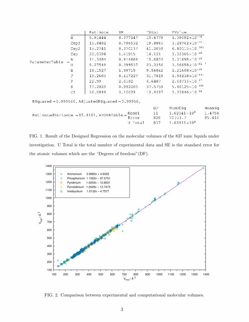
FIG. 1. Result of the Designed Regression on the molecular volumes of the 837 ionic liquids under

investigation. U Total is the total number of experimental data and SE is the standard error for

the atomic volumes which are the “Degrees of freedom”(DF).

100

200

300

400

500

600

700

800

900

1000

1100

1200

1300

1400

100 200 300 400 500 600 700 800 900 1000 1100 1200 1300 1400

Vex

p / Å

3

Vmol / Å 3

Ammonium 0.9983x + 4.6333

Phosphonium 1.1002x − 97.5751

Pyridinium 1.0253x − 12.8531

Pyrrolidinium 1.0029x − 12.7473

Imidazolium 1.0133x − 4.7577

FIG. 2. Comparison between experimental and computational molecular volumes.

3

Fig. 2 correlates experimental molecular volumes with the predictions based on the De-

signed regression values of the atomic volumes. The magenta line represents 100% agree-

ment. The legend also contains linear regression of the corresponding ionic liquid classes. A

slope of 1.0 and an axis intercept of 0.0 would correspond to 100% agreement.

In a second step, the Lorentz-Lorenz equation is used to compute experimental molecular

polarizabilities.n2

D − 1

n2D + 2

=4π

3

αmol

Vmol

(2)

Since many groups report the density or the refractive index of an ionic liquid but seldom

both values, the set of ionic liquids to compute the molecular volume differs from that to

evaluate the molecular polarizabilities. Therefore, the values of Vmol in Eq. (2) are predicted

by the Designed Regression. Afterwards, the Designed Regression is applied to the molecular

polarizabilities:

α1

mol

α2mol

...

αmmol

=

X1

H X1B X1

C(sp3) X1C(sp2) X

1C(sp) X1

N X1O X1

F X1P X1

S X1Cl

X2H X2

B X2C(sp3) X

2C(sp2) X

2C(sp) X2

N X2O X2

F X2P X2

S X2Cl

......

......

......

......

......

...

XmH Xm

B XmC(sp3) X

mC(sp2) X

mC(sp) X

mN Xm

O XmF Xm

P XmS Xm

Cl

·

αH

αB

αC(sp3)

αC(sp2)

αC(sp)

αN

αO

αF

αP

αS

αCl

(3)

yielding the following atomic polarizabilities:

4

FIG. 3. Result of the Designed Regression on the molecular polarizabilities of the 414 ionic liquids

under investigation.

0

10

20

30

40

50

60

70

80

0 10 20 30 40 50 60 70 80

α e

xp /

Å 3

α mol / Å 3

Ammonium 0.9996x + 0.0761

Phosphonium 0.9854x + 1.8932

Pyridinium 1.0242x − 0.0303

Pyrrolidinium 1.0375x − 0.7061

Imidazolium 0.9957x + 0.0910

FIG. 4. Comparison between experimental and computational molecular polarizabilities.

5

MODEL OF THE EXCESS ELECTRON

The molecular polarizabilities αmol in Table I were computed by MP2/aug-cc-pVDZ and

CCSD(T)/aug-cc-pVQZ for neutral and charged ionic liquid related compounds. The agree-

ment between the quantum-chemical results indicates that MP2/aug-cc-pVDZ seems to be

sufficient to compute reasonable molecular polarizabilities as visible in Fig. 5. Ref. 6 showed

that using HF or smaller basis sets, e.g. 6-311+G(3df,2p), result in lower predictions of αmol.

1

2

3

4

5

6

7

8

9

10

1 2 3 4 5 6 7 8 9 10

αC

CS

D(T

)/au

g−cc

−pV

QZ /

Å 3

αMP2/aug−cc−pVDZ / Å 3

neutral moleculescationsanions

FIG. 5. Comparison between quantum-chemical calculations of the molecular polarizability at

MP2/aug-cc-pVDZ and CCSD(T)/aug-cc-pVQZ level. The dashed line represents 100% agreement.

6

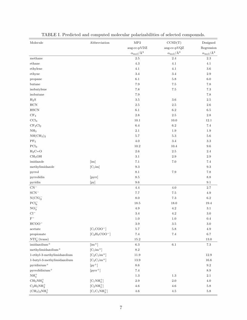
TABLE I. Predicted and computed molecular polarizabilities of selected compounds.

Molecule Abbreviation MP2 CCSD(T) Designed

aug-cc-pVDZ aug-cc-pVQZ Regression

αmol/A3 αmol/A3 αmol/A3

methane 2.5 2.4 2.3

ethane 4.3 4.1 4.1

ethylene 4.1 4.1 3.6

ethyne 3.4 3.4 2.9

propane 6.1 5.8 6.0

butane 7.9 7.5 7.8

isobutylene 7.8 7.5 7.3

isobutane 7.9 7.8

H2S 3.5 3.6 2.5

HCN 2.5 2.5 2.6

HSCN 6.1 6.2 6.5

CF4 2.8 2.5 2.8

CCl4 10.1 10.0 12.1

CF2Cl2 6.4 6.2 7.4

NH3 2.1 1.9 1.9

NH(CH3)2 5.7 5.3 5.6

PF5 4.0 3.4 3.3

PCl3 10.2 10.4 9.6

H2C=O 2.6 2.5 2.4

CH3OH 3.1 2.9 2.9

imidazole [im] 7.1 7.0 7.4

methylimidazole [C1im] 9.3 9.3

pyrrol 8.1 7.9 7.8

pyrrolidin [pyrr] 8.5 8.8

pyridin [py] 9.6 9.1

CN− 4.4 4.0 2.7

SCN− 7.7 7.5 4.9

N(CN)−2 8.0 7.3 6.2

PCl−6 18.5 18.0 19.4

NO−3 4.9 4.2 3.1

Cl− 3.4 4.2 3.0

F− 1.0 1.0 0.4

HCOO− 3.9 3.5 3.0

acetate [C1COO−] 5.7 5.8 4.9

propionate [C2H5COO−] 7.4 7.4 6.7

NTf−2 (trans) 15.2 13.0

imidazolium+ [im+] 6.3 6.1 7.3

methylimidazolium+ [C1im+] 8.2

1-ethyl-3-methylimidazolium [C2C1im+] 11.9 12.9

1-butyl-3-methylimidazolium [C4C1im+] 13.9 16.6

pyridinium+ [py+] 8.6 9.2

pyrrolidinium+ [pyrr+] 7.4 8.9

NH+4 1.3 1.3 2.1

CH3NH+3 [C1NH+

3 ] 2.9 2.0 4.0

C2H5NH+3 [C2NH+

3 ] 4.6 4.6 5.8

(CH3)2NH+2 [C1C1NH+

3 ] 4.6 4.5 5.8

7

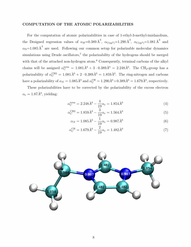
COMPUTATION OF THE ATOMIC POLARIZABILITIES

For the computation of atomic polarizabilities in case of 1-ethyl-3-methyl-imidazolium,

the Designed regression values of αH=0.389 �A3, αC(sp2)=1.290 �A3

, αC(sp3)=1.081 �A3and

αN=1.085 �A3are used. Following our common setup for polarizable molecular dynamics

simulations using Drude oscillators,7 the polarizability of the hydrogens should be merged

with that of the attached non-hydrogen atom.8 Consequently, terminal carbons of the alkyl

chains will be assigned αtermC = 1.081A3 + 3 · 0.389A3 = 2.248A3. The CH2-group has a

polarizability of αCH2C = 1.081A3 + 2 · 0.389A3 = 1.859A3. The ring-nitrogen and carbons

have a polarizability of αN = 1.085A3 and αCHC = 1.290A3+0.389A3 = 1.679A3, respectively.

These polarizabilities have to be corrected by the polarizability of the excess electron

αe = 1.87A3, yielding:

αtermC = 2.248A3 − 4

19αe = 1.854A3 (4)

αCH2C = 1.859A3 − 3

19αe = 1.564A3 (5)

αN = 1.085A3 − 1

19αe = 0.987A3 (6)

αCHC = 1.679A3 − 2

19αe = 1.482A3 (7)

8

REFERENCES

1Wolfram Research, Inc., Mathematica, Champaign, Illinois, version 9.0 ed. (2012).

2S. R. Searle, Linear models for unbalanced data (John Wiley & Sons, New York, 1987).

3J. D. Jobson, Applied multivariate data analysis volume 1: Regression and experimental

design (Springer-Verlag, New York, 1991).

4H. Sahai and M. Ageel, The analysis of variance: Fixed, random and mixed models

(Birkhauser, Boston, 2000).

5R. Nisbet, J. Elder, and G. Miner, Statistical analysis and data mining (Academic press,

Elsevier, 2009).

6E. I. Izgorodina, M. Forsyth, and D. R. MacFarlane, Phys. Chem. Chem. Phys. 11, 2452

(2009).

7C. Schroder and O. Steinhauser, J. Chem. Phys. 133, 154511 (2010).

8M. Schmollngruber, V. Lesch, C. Schroder, A. Heuer, and O. Steinhauser, Phys. Chem.

Chem. Phys. 17, 14297 (2015).

9