Embed Size (px)
Citation preview

Thomas Würthinger
Visualization of Program Dependence Graphs
A thesis submitted in partial satisfaction of the requirements for the degree of
Master of Science
(Diplom-Ingenieur)
Supervised by: o.Univ.-Prof. Dipl.-Ing. Dr. Dr.h.c. Hanspeter Mössenböck
Dipl.-Ing. Christian Wimmer
Institute for System Software Johannes Kepler University Linz
Linz, August 2007
Johannes Kepler University Linz A-4040 Linz • Altenberger Straße 69 • Internet: http://www.jku.at • DVR 0093696

Abstract
The Java HotSpotTM server compiler of Sun Microsystems uses intermediate graph data struc-tures when compiling Java bytecodes to machine code. The graphs are program dependencegraphs, which model both data and control dependencies. Fordebugging, there are built-intracing mechanisms that output a textual representation ofthe graphs to the command line.
This thesis presents a tool which displays the graphs of the server compiler. It records inter-mediate states of the graph during the compilation of a method. The user can then navigatethrough the graph and apply rule-based filters that change the appearance of the graph. The toolcalculates an approximation of the control flow to cluster the nodes of the graph into blocks.
Using a visual representation of the data structures speedsup debugging and helps understand-ing the code of the compiler. The thesis describes the code added to the server compiler andthe Java application that displays the graph. Additionally, the server compiler and the NetBeansplatform are outlined in general.
Kurzfassung
Der Java HotSpotTM Server Compiler von Sun Microsystems benutzt Graphen als temporäreDatenstrukturen beim Kompilieren von Java Bytecodes zu Maschinencode. Die Graphen desCompilers sind Programmabhängigkeitsgraphen, mit denen sowohl der Kontrollfluss als auchdie Datenabhängigkeiten modelliert werden. Für die Suche von Fehlern kann eine textuelleRepräsentation der Graphen auf die Kommandozeile ausgegeben werden.
Diese Arbeit beschreibt ein Programm zur Anzeige der Graphen des Server Compilers. Bei derKompilierung einer Methode werden Zustände des Graphen aufgezeichnet. Der Benutzer kanndurch den Graphen navigieren und regelbasierte Filter anwenden, um die graphische Anzeigedes Graphen zu verändern. Das Programm berechnet eine Annäherung des Kontrollflusses, umdie Knoten in Blöcke zu gruppieren.
Die Verwendung einer graphischen Repräsentation der Datenstrukturen beschleunigt die Fehler-suche und hilft den Quelltext des Compilers zu verstehen. Die Arbeit behandelt den Quell-text, der zum Server Compiler hinzugefügt wurde, und die Java Anwendung, die den Graphenanzeigt. Weiters werden der Server Compiler und die NetBeans Plattform beschrieben.

Contents
1 Introduction 1
1.1 Class Diagram Legend . . . . . . . . . . . . . . . . . . . . . . . . . . . . . .2
1.2 Related Work . . . . . . . . . . . . . . . . . . . . . . . . . . . . . . . . . . . 2
2 NetBeans 4
2.1 Why NetBeans? . . . . . . . . . . . . . . . . . . . . . . . . . . . . . . . . . . 4
2.2 History . . . . . . . . . . . . . . . . . . . . . . . . . . . . . . . . . . . . . . 5
2.3 Modular Design . . . . . . . . . . . . . . . . . . . . . . . . . . . . . . . . . . 6
2.4 Filesystem . . . . . . . . . . . . . . . . . . . . . . . . . . . . . . . . . . . . . 7
2.5 Lookup . . . . . . . . . . . . . . . . . . . . . . . . . . . . . . . . . . . . . . 8
2.6 Visual Library . . . . . . . . . . . . . . . . . . . . . . . . . . . . . . . . . . . 9
3 Server Compiler 12
3.1 The Java HotSpotTM VM . . . . . . . . . . . . . . . . . . . . . . . . . . . . . 12
3.1.1 Client versus Server Compiler . . . . . . . . . . . . . . . . . . . .. . 13
3.1.2 Java Execution Model . . . . . . . . . . . . . . . . . . . . . . . . . . 14
3.2 Architecture of the Server Compiler . . . . . . . . . . . . . . . . .. . . . . . 15
3.3 Ideal Graph . . . . . . . . . . . . . . . . . . . . . . . . . . . . . . . . . . . . 16
3.3.1 Data Dependence . . . . . . . . . . . . . . . . . . . . . . . . . . . . . 17
3.3.2 Empty Method . . . . . . . . . . . . . . . . . . . . . . . . . . . . . . 17
3.3.3 Phi and Region Nodes . . . . . . . . . . . . . . . . . . . . . . . . . . 18
3.3.4 Safepoint Nodes . . . . . . . . . . . . . . . . . . . . . . . . . . . . . 20
3.4 Optimizations . . . . . . . . . . . . . . . . . . . . . . . . . . . . . . . . . . .21
3.4.1 Identity Optimization . . . . . . . . . . . . . . . . . . . . . . . . . .. 21
i

3.4.2 Constant Folding . . . . . . . . . . . . . . . . . . . . . . . . . . . . . 22
3.4.3 Global Value Numbering . . . . . . . . . . . . . . . . . . . . . . . . . 22
3.4.4 Loop Transformations . . . . . . . . . . . . . . . . . . . . . . . . . . 23
3.5 MachNode Graph . . . . . . . . . . . . . . . . . . . . . . . . . . . . . . . . . 24
3.6 Register Allocation . . . . . . . . . . . . . . . . . . . . . . . . . . . . . .. . 26
4 User Guide 28
4.1 Generating Data . . . . . . . . . . . . . . . . . . . . . . . . . . . . . . . . . .29
4.2 Viewing the Graph . . . . . . . . . . . . . . . . . . . . . . . . . . . . . . . . 30
4.3 Navigating within the Graph . . . . . . . . . . . . . . . . . . . . . . . .. . . 31
4.4 Control Flow Window . . . . . . . . . . . . . . . . . . . . . . . . . . . . . . 32
4.5 Filters . . . . . . . . . . . . . . . . . . . . . . . . . . . . . . . . . . . . . . . 32
4.6 Bytecode Window . . . . . . . . . . . . . . . . . . . . . . . . . . . . . . . . . 36
5 Visulializer Architecture 37
5.1 Module Structure . . . . . . . . . . . . . . . . . . . . . . . . . . . . . . . . .37
5.2 Graph Models . . . . . . . . . . . . . . . . . . . . . . . . . . . . . . . . . . . 39
5.2.1 XML File Structure . . . . . . . . . . . . . . . . . . . . . . . . . . . . 40
5.2.2 Display Model . . . . . . . . . . . . . . . . . . . . . . . . . . . . . . 42
5.2.3 Layout Model . . . . . . . . . . . . . . . . . . . . . . . . . . . . . . . 43
5.3 Properties and Selectors . . . . . . . . . . . . . . . . . . . . . . . . . .. . . . 45
5.4 Filters . . . . . . . . . . . . . . . . . . . . . . . . . . . . . . . . . . . . . . . 46
5.5 Difference Algorithm . . . . . . . . . . . . . . . . . . . . . . . . . . . . .. . 48
6 Hierarchical Graph Layout 50
6.1 Why Hierarchical? . . . . . . . . . . . . . . . . . . . . . . . . . . . . . . . .50
6.2 Processed Steps . . . . . . . . . . . . . . . . . . . . . . . . . . . . . . . . . .51
6.3 Breaking Cycles . . . . . . . . . . . . . . . . . . . . . . . . . . . . . . . . . .53
6.4 Assign Layers . . . . . . . . . . . . . . . . . . . . . . . . . . . . . . . . . . . 55
6.5 Insert Dummy Nodes . . . . . . . . . . . . . . . . . . . . . . . . . . . . . . . 56
6.6 Assign Y-Coordinates . . . . . . . . . . . . . . . . . . . . . . . . . . . . .. . 57
6.7 Crossing Reduction . . . . . . . . . . . . . . . . . . . . . . . . . . . . . . .. 58
ii
6.8 Assign X-Coordinates . . . . . . . . . . . . . . . . . . . . . . . . . . . . .. . 60
6.8.1 DAG Method . . . . . . . . . . . . . . . . . . . . . . . . . . . . . . . 60
6.8.2 Rubber Band Method . . . . . . . . . . . . . . . . . . . . . . . . . . . 62
6.9 Cluster Layout . . . . . . . . . . . . . . . . . . . . . . . . . . . . . . . . . . 64
6.10 Drawing of Backedges . . . . . . . . . . . . . . . . . . . . . . . . . . . . .. 65
6.11 Optimization for Large Graphs . . . . . . . . . . . . . . . . . . . . .. . . . . 66
7 Compiler Instrumentation 67
7.1 Overview . . . . . . . . . . . . . . . . . . . . . . . . . . . . . . . . . . . . . 67
7.2 Identifying Blocks . . . . . . . . . . . . . . . . . . . . . . . . . . . . . . .. 68
7.3 Building Dominator Tree . . . . . . . . . . . . . . . . . . . . . . . . . . .. . 70
7.4 Scheduling . . . . . . . . . . . . . . . . . . . . . . . . . . . . . . . . . . . . 73
7.5 Adding States . . . . . . . . . . . . . . . . . . . . . . . . . . . . . . . . . . . 74
8 Conclusions 75
iii

Chapter 1
Introduction
When compiling Java methods to machine code, the Java HotSpotTM server compiler of SunMicrosystems uses an intermediate representation that corresponds to a directed graph. Severalnodes are added to the graph for every bytecode. Afterwards,transformations are applied to thegraph with the goal to increase the execution speed of the method. After all optimizations areapplied, the graph is converted to code that can be directly executed on the target machine. Thegraph is complex for large methods. It is difficult to understand the purpose of a certain nodein the graph because of the high number of applied optimizations. Currently, developers usecode that prints the graph on the command line when they are debugging the server compiler.This thesis presents a tool that helps the developer understand the graph by giving a visualrepresentation of it.
The user can specify rule-based filters, which change the appearance of the graph. Differentfilters can be used when different properties of the graph areof interest. Navigation mechanismsare available, such that the user can focus on specific parts of a large graph. An additional featureof the tool is to display the differences between two graphs.
This thesis is divided into eight chapters. Alongside the introduction these chapters are: Chap-ter 2 describes the NetBeans platform in general. The program that displays the graph is basedon the NetBeans platform. Some important concepts of NetBeans and the visual library of Net-Beans are explained. Chapter 3 outlines the server compiler. The general architecture and thedifferences to the client compiler are presented. The focusof the chapter lies on the graph datastructure and the optimizations applied by the compiler.
Chapter 4 is a user guide for the visualization tool. It explains how to connect the server com-piler to the Java program. The navigation possibilities, the filters, the Control Flow Window,and the Bytecode View Window are described.
Chapter 5 presents the architecture of the Java applicationthat displays the graph. The datamodels and the class structure are outlined. Chapter 6 is a description of the hierarchical layoutalgorithm used to find coordinates for the nodes of the graph and interpolation points for theedges.
1

Introduction Class Diagram Legend
Chapter 7 presents the C++ code added to the server compiler.This code is responsible forthe scheduling and for saving the state of the graph during the compilation of methods. Chap-ter 8 describes the main difficulties during development of the tool and points out extensionpossibilities.
1.1 Class Diagram Legend
The class diagrams in this thesis follow the conventions shown in Figure 1.1. Interfaces areorange boxes with an italic name of the interface in it. Greenboxes are classes which are partof a previously explained or external API. The connections of the current classes with them arepart of the drawing. Generally, classes that are strongly related are grouped using a roundedrectangle with a dashed border.
For inheritance and composition, the standard UML symbols are used. When no cardinality isspecified at the start or end of a composition, then the cardinality is 1. The blue arrow meansthat the source uses the destination of the arrow. A textual attribute classifies the relation further.
boolean edit()
EditFilterCookie
has-a relation
default cardinality = 1uses relation
group of related classes
inheritance
ScriptEngine
interfaceclass of external or
previously explained API
Figure 1.1: Conventions used in the class diagrams.
1.2 Related Work
A debugging tool for the HotSpotTM client compiler [17] visualizes three different data struc-tures: The control flow graph, the data dependence graph, andinformation about the registerallocation. The data is traced by the compiler in a textual format. In contrast to the tool pre-sented in this thesis, a direct communication between the compiler and the application is notpossible.
Stefan Loidl presents the data dependence graph visualizerof the tool [20]. It displays the datadependencies of the intermediate representation of the client compiler. In comparison to thegraph of the server compiler, the data dependence graph of the client compiler is more sparse.
2

Introduction Related Work
As most of the nodes have only few incoming edges, the tool does not need to define slots todistinguish between them.
The author’s bachelor thesis [32] presents a visualizer forJava control flow graphs, which isalso part of the client compiler visualization application. The graph is recorded at several stagesduring compilation. The control flow graph of the client compiler is simpler than the graph ofthe server compiler, because it contains only control flow dependencies and no data dependen-cies. Additionally, there is not a node for every instruction, but for every block of instructions.This significantly reduces the size of the graph. Therefore,some of the advanced navigationand filtering concepts are not necessary for the control flow graph.
Several software products can draw arbitrary graph structures. The development of a specificvisualization tool for the server compiler has the advantage that the layout and the navigationis adapted to the needs of the graph of the server compiler. The following list presents threetools that can be used to draw graphs automatically. Features such as filtering or fast navigationwithin the graph are not available in these tools.
Graph Visualization Software (GraphViz) [13]: GraphViz is a group of open source pro-grams that visualize directed graphs, which are specified ina textual format. The exe-cutabledot.exe is part of the GraphViz group and converts the textual representationof a directed graph into an image file. The hierarchical layout algorithm presented in thisthesis is based on the algorithm used by GraphViz. The main purpose of GraphViz is notto interactively view the graph, but to produce a static image file for the graph. Enhance-ments to the GraphViz layout algorithm presented in this thesis are the cutting of edgesand a second way to assign x-coordinates to the nodes based onthe rubber band method.Additionally, backward edges are treated by the visualization tool in a special way.
aiSee Graph Layout Software [14]: aiSee is a commercial graph layout software that is a suc-cessor of the free tool Visualization of Compiler Graphs (VCG) [27] developed by GeorgSander. It is not specialized on hierarchical graph layout,but enables the user to choosefrom different layout algorithms including force directedlayout. It supports clusteringand folding of the graph. The tool uses a custom input format for the graphs.
uDraw [30]: The uDraw graph visualization software is developed at the University of Bremenand is specialized on hierarchical layout. One of the key features is that the user can, undersome restrictions, manually change the layout after the automatic algorithm was applied.
3

Chapter 2
NetBeans
NetBeans [22] is anintegrated development environment(IDE) written in Java. It is an opensource project highly supported by Sun Microsystems. Although it is mainly designed to sup-port developers in creating Java applications, it can also be used for C/C++ projects. Addition-ally, there are extensions available for NetBeans that allow to use the IDE also for completelydifferent purposes like UML modeling, scripting in Ruby or Groovy, creating LaTeX docu-ments, and so on. The visualization tool uses the NetBeans core libraries as a platform forbuilding rich client applications with Java.
This chapter explains some important concepts of NetBeans that are used by the visualizationtool. It gives a short overview of the NetBeans platform for software developers who are usingNetBeans as the basis for their application [2]. If you are looking for a description of NetBeansas a development environment, see [21].
2.1 Why NetBeans?
Building upon a platform instead of using only plain Swing speeds up the development of a Javaapplication and prevents developers from reinventing the wheel over and over again. How canan application benefit from using the NetBeans platform as anunderlying layer? The followinglist introduces some useful aspects of the NetBeans library. The most important of them will beexplained in detail in upcoming sections.
Module: NetBeans itself can be seen as a collection of Java modules that have well-defineddependencies. It is assured that only the modules currentlyneeded are loaded. Thisimproves memory usage as well as the startup time of an application. Additionally, de-velopers are enforced to develop modular applications, which leads to a better design ingeneral.
Window System: The built-in windowing system allows docking of componentsand supportstabbing of multiple documents. Additionally, actions thatoperate on the global selection
4

NetBeans History
can be declared. Only using Swing means that either such functionality does not exist orit must be implemented by hand, highly increasing the total development effort.
Persistence: Configuration and serialization data is organized in virtual filesystems. When theNetBeans application is not running, the data is stored in a filesystem on the hard disk.
Visual Library: The NetBeans platform comes with a high-level drawing library. It is espe-cially useful for the visualization tool as it is designed todraw graphs. It can add a largeset of features to a drawing application for "free", at leastfor just adding a few lines ofJava code. Examples for such functionalities are zooming, satellite view, and animation.
Java libraries with the same functionality that are not partof the NetBeans platform could beused, it is however more convenient if the libraries are directly integrated into the platform. Thisallows the libraries to work together without compatibility conflicts. Additionally, all NetBeanslibraries take benefit of the module system, which manages lazy loading of the modules. Thedrawback of using a large amount of underlying libraries fora project is a higher developmenttime needed at the beginning of a project, because the developer needs to get familiar with thelibraries. However, for larger projects this additional cost pays off in the long run. Additionally,this cost needs not be paid when subsequent projects also take benefit of the same libraries. Sobuilding the first application on top of NetBeans means at first doing additional work, but thelonger one uses the platform, the bigger are the advantages [2].
2.2 History
The first code for the system that evolved over more than a decade to the current version 5.5of NetBeans was written in 1996. It was a student project, whose intention was to build anintegrated development environment by using only Java code. At this time the program wascalled Xelfi [33]. For producing the screenshot of Xelfi shownin Figure 2.1, installing theold JDK version 1.1 was necessary. The NetBeans of today and Xelfi have only few thingsin common, but some of the basic design concepts have never changed since the early days.Among them are the modular design and the concept of virtual filesystems. Xelfi soon becamea success and therefore a company named after the IDE was founded. During these days thecurrent name of NetBeans was introduced: One of the businessideas was to developnetwork-enabled JavaBeans.
In 1999, Sun Microsystems, the founder of the Java programming language, acquired the com-pany. The company was interested in NetBeans and so the product forms their flagship Java IDEuntil nowadays. Sun soon realized that the growth of NetBeans can be accelerated by buildinga development community around it, instead of distributingit as a commercial product. There-fore, they open-sourced the whole IDE in 2000. After this step, people started using NetBeansnot only as an IDE, but also as a library to build their own applications. This brought up theidea of a rich client platform.
5

NetBeans Modular Design
Figure 2.1: Screenshot of Xelfi, the ancestor of NetBeans, running with JDK 1.1.
The number of NetBeans users grows steadily. The current stable version of NetBeans is 5.5,but there is already a pre-release version of NetBeans 6.0 available. The development of thevisualization tool started with NetBeans 5.5, but later on it was ported to NetBeans 6.0. [1]
2.3 Modular Design
NetBeans applications consist of separate modules workingtogether to form one big program.The IDE itself is a set of NetBeans modules that support developers at programming in Java.There are some official extensions available like a profiler,special support for mobile applica-tion development, and C/C++ programming. Various modules developed by other companiescan also enrich the IDE. The NetBeans platform consists of a set of modules that manage theco-operation between the modules and also provide some basic concepts regarding data storageand the user interface.
A NetBeans module is defined by a JAR file with additional information in the manifest. It hasa version and specifies on which modules it depends, e.g. which modules need to be availablefor running this module. Modules can be enabled and disabledwhile the application is running.Such components are also calledplug-insas they resemble a plug. In NetBeans, the term plug-inis reserved for a collection of modules that are deployed as one unit.
Each module has a custom classloader, which searches for classes only in the standard Javaclasspath and in the modules that are listed as dependencies. The minimum version of a re-quired module is defined when declaring dependencies. Additionally, there must not be anycyclic dependencies. A module must explicitly declare which packages are accessible by othermodules. The usage of public classes declared outside of these declared packages is not pos-sible. A lazy loading mechanism for the modules helps reducing memory usage and startuptime.
6

NetBeans Filesystem
2.4 Filesystem
One of the base concepts of module interaction in a NetBeans application uses virtual filesys-tems. A module can define an XML layer file to add declarative data to thesystem filesystem,i.e. a virtual filesystem that is shared among all modules. Atstartup, the filesystems of theindividual modules are merged into the system filesystem. Entries in the filesystem can bedirectories, virtual files or pointers to real files. Virtualfiles consist of a name and a set ofkey-value pairs that are defined in the XML layer file.
Listing 2.1 shows an example layer file describing the filesystem of a module. It is a simplifiedversion of one of the layer files used by the visualization tool. An application can use the systemfilesystem for example to register windows or to add actions to the toolbar and the menu bar.
Actions are registered as files in the filesystem in the folderActions. The module responsiblefor instantiating the action objects scans through this folder. The name of a file specifies theclass that represents the action, in this example the classImportAction. An action can beregistered as a menu item by adding an entry to the folderMenu. As the import action shouldappear in the file menu, it is added to the subfolderFile.
There should only be one instance of classImportAction in the system, so we use a shad-owing mechanism that functions similar to link files. The extension.shadow specifies thatthe file points to another file and the attributeoriginalFile specifies the destination of thepointer. There is also a mechanism available for hiding files. To remove the standard open menuitem from the file menu, we simply hide the file that defines thatmenu item by declaring a filewith the extension.instance_hidden.
Listing 2.1 An XML layer file defining an action and hiding a menu item.<?xml version="1.0" encoding="UTF-8"?><!DOCTYPE filesystem PUBLIC "-//NetBeans//DTD Filesystem 1.1//EN""http://www.netbeans.org/dtds/filesystem-1_1.dtd">
<filesystem><folder name="Actions">
<folder name="File"><file name="at-ssw-ImportAction.instance"/>
</folder></folder><folder name="Menu">
<folder name="File"><file name="at-ssw-ImportAction.shadow">
<attr name="originalFile" stringvalue="Actions/Edit/at-ssw-ImportAction.instance"/>
</file><file name="org-netbeans-modules-openfile-
OpenFileAction.instance_hidden"/></folder>
</folder></filesystem>
7

NetBeans Lookup
The filesystem is also used to save the state of a NetBeans application after shutdown. Asubdirectory of the user directory is used to save the data. In this case the filesystem is notrepresented by an XML file, but by a directory structure that is physically present on the harddisk. At startup, the user-specific filesystem is merged withthe filesystems of the modules.
2.5 Lookup
Another mechanism that is specific to NetBeans is the conceptof lookup. The idea behindlookup is to change the set of interfaces that an object provides during program execution. InJava it is only possible to declare interfaces for classes atcompile time. This set cannot bechanged later on. It is also impossible that a certain objectof a class implements an interfaceand another one does not.
The interfaceLookup defines functions that return a collection of objects compatible to thetype specified as a parameter. This way it is possible to ask theLookup object if it can providean implementation of a certain interface. The object can return itself or any other existingor newly created object, the only restriction is that the returned object must implement theinterface.
An example for the use of the lookup mechanism is how the save menu item and an editor of afile interact. The save menu item does not know how to save a certain file type. Everything itneeds to do is checking whether it is currently possible to save a file and trigger the save processwhen the menu item is clicked.
Lookup getLookup()
GraphEditor
void save()
GraphSaveCookie
void save()
SaveCookie
SaveAction
Lookup getLookup()
Lookup.Provider
creates
find active editor ask lookup for an implementation of
Service User
Shared Interfaces
Service Provider
Figure 2.2: Using lookup, there is no dependency between service user and service provider.
Figure 2.2 shows how the classes are related. The interfaceLookup.Provider is part of thestandard NetBeans API and is implemented by objects that provide a lookup. In this case, theservice is defined by the interfaceSaveCookie with a method that can be used for saving.
8

NetBeans Visual Library
TheSaveAction object first retrieves the lookup of the active editor and asks for an object ofkindSaveCookie. When the editor cannot provide the service, it returnsnull and the menuitem is disabled. Otherwise it returns an object that implements the interface and that can beused by the menu item in case the user clicks it.
The figure also shows how the classes can be separated in threedifferent modules. One modulejust contains the declaration of the service. Provider and user of the service only need to dependon this API module and need no dependencies among each other.While the service user andthe service provider are able to work together, none of them depends on the other.
There are several additional classes that enrich the lookupfunctionality. It is possible to monitorthe lookup of an object by installing listeners. The classProxyLookup allows to combine thelookups of several objects into a single one. A list component, for example, proxies the lookupof the currently selected nodes. So a pattern similar to the save mechanism can be used for anyaction that works with the elements of the list. The action declares the interface that an objectmust provide that the action can work. It will get enabled anddisabled depending on the currentselection of the list.
The NetBeans platform predefines two global lookup objects.One can be reached by callingLookup.getDefault() and represents the global system lookup. The other one is oftenused by actions that depend on the current active window. It can be accessed using the methodUtilities.actionsGlobalContext(). It proxies the lookup of the window that iscurrently focused. When the user activates another window,this lookup is changed. Reactingon changes can be done by adding listeners to lookup objects.The visualization tool usesthis mechanism to always display the properties of the selected objects of the currently activewindow in the Properties Window.
The Node class is closely related to the lookup mechanism. A node can have an unlimitednumber of child nodes but only one parent node, so they form a tree-like structure. The childrenof a node are only accessed when the node is expanded by the user. There are several compo-nents such as a treeview or a list that are able to use such a tree of nodes as their model. Thesecomponents provide a proxy lookup that combines the lookupsof the currently selected nodes.The visualization tool uses the Node API in the Outline and inthe Bytecode Window.
2.6 Visual Library
The NetBeans visual library is a high-level graphical framework built on top of Swing andJava2D. It is designed to support applications that need to display editable graphs such as UMLdiagrams. The library can also be used by applications that are not built upon the NetBeansplatform.
Figure 2.3 shows a class diagram of the most important classes of the visual library and howthey interact. Graphical components are calledwidgetsand are organized in a tree hierarchy.The topmost widget is always ascene. This widget forms the bridge between Swing and thevisual library. A scene can create aJComponent object that displays the contents of the
9

NetBeans Visual Library
scene. In contrast to Swing components, widgets need not have a rectangular shape. There isa predefined mechanism for drawing a connection between two widgets. A connection has asource and a target anchor that are both related to some widget.
Scene
Widget
ConnectionWidget
Anchor
WidgetAction
JComponentcreates Swing component
children
source and target anchor
*
2
*
*
* *
related anchors
SceneAnimator
Figure 2.3: Class diagram of the NetBeans visual library.
A widget has anaction mapassociated with it, i.e. a list of objects of typeWidgetActionthat can react on GUI events. There are a lot of predefined actions that automatically performfor example moving, selecting or resizing of a widget triggered by user input. The built-inanimation mechanisms can be used to move widgets smoothly and to let them fade in or out.
Additionally there are some high-level functions built into theScene class that allow zoomingwith different levels of details and the automatic construction of satellite views. Listing 2.2shows the power of the Visual Library in an example. The result is a label that can be zoomedand that changes its background color when it is double clicked. A screenshot of the result-ing program is shown in Figure 2.4. The NetBeans libraries that are needed for running thisapplication areorg-openide-util.jar andorg-netbeans-api-visual.jar.
Figure 2.4: Screenshot of the visual library example program during execution.
First, the application creates aScene object and adds aWidgetAction that allows the userto zoom using the mouse wheel. It constructs aLabelWidget and adds it as a child to thescene. Then it constructs aWidgetAction that calls anEditProvider when a widgetis double clicked. This action is added to the label. An action can be added to any number
10

NetBeans Visual Library
of widgets. As the scene itself also represents a widget, thescene itself would also change itsbackground on double click when the example action was addedto it. Finally a swingJFramecomponent is created, and the view of the scene is added to this window.
Listing 2.2 Java source code of a visual library program with a label widget and an action.public class VisualExample {
// Create edit actionWidgetAction editAction = ActionFactory.createEditAction(
new EditProvider() {public void edit(Widget w) {
w.setBackground(Color.RED);}
});
public static void main(String[] args) {
// Create scene object and assign zoom actionScene s = new Scene();s.getActions().addAction(ActionFactory.createZoomAction());
// Create label widgetLabelWidget l = new LabelWidget(s, "Hello world!");s.addChild(l);l.setOpaque(true);
// Add action to labell.getActions().addAction(editAction);
// Create swing frameJFrame f = new JFrame();f.setSize(200, 100);f.setDefaultCloseOperation(JFrame.EXIT_ON_CLOSE);
// Add scene viewf.add(s.createView());f.setVisible(true);
}}
11

Chapter 3
Server Compiler
The visualization tool improves the abilities to analyze internal data structures of the JavaHotSpotTM server compiler [23], which is part of the Java HotSpotTM Virtual Machine of SunMicrosystems. A virtual machine (VM) acts as a bridge between a program and the operatingsystem. The primary purpose of VMs is to enable the creation of platform-independent appli-cations. In the beginning of this chapter the Java HotSpotTM VM is described in general, lateron the main data structure of the server compiler and some of the most important optimizationsteps are presented.
3.1 The Java HotSpotTM VM
The Java HotSpotTM VM is a virtual machine developed by Sun Microsystems that implementsthe Java Virtual Machine Specification [29]. Figure 3.1 shows the main components of this VM.Basically Java methods are executed by the interpreter. When a method is invoked a specificnumber of times, the just-in-time compiler produces machine code for the method. Later callsof the method jump to the compiled machine code and will therefore run faster. The reasonwhy a method is not immediately compiled to machine code at the first execution is that mostJava methods are executed so infrequently that compiling them does not pay off. Depending onwhether the virtual machine is started with the flag-server or not, the server compiler or theclient compiler [15][18] is chosen to do the compilation task.
There are some cases in which the compiled machine code of a method can no longer be usedand execution continues in the interpreter. Such cases occur when a compiler makes an opti-mistic assumption to produce faster code. When the assumption is later invalidated, e.g. becauseof dynamic class loading, the machine code is no longer usable. Jumping from the interpreterto the compiler and vice versa is not only possible at the invocation of a method, but also duringthe execution. Reverting back from the compiled machine code to the interpreter can be doneat specific points of a method calledsafepoints. This process is calleddeoptimization.
12

Server Compiler The Java HotSpotTM VM
There is also an opposite of deoptimization calledon-stack-replacement. Imagine a method thatis executed only once but consists of a long-running loop. Running the whole loop in the inter-preter would heavily decrease execution speed. Therefore,the interpreter does not only countthe invocations of a method, but also how often a backward jump occurs. When this counterexceeds a specific threshold, the method is compiled with a special on-stack-replacement en-try. At this entry, machine instructions for loading the current values from the interpreter areinserted.
Interpreter
Garbage Collector
Runtime Client Compiler
Server Compiler
Compilation
Deoptimization
Just-In-Time
Compilers
Figure 3.1: Architecture of the Java HotSpotTM Virtual Machine.
3.1.1 Client versus Server Compiler
The difference between client and server compiler is that the client compiler focuses on highcompilation speed, while the focus of the server compiler lies on peak performance. The clientcompiler performs only a limited set of optimizations and isbest-suited for short-running clientapplications. The server compiler needs more time for compilation, but produces more opti-mized machine code, so the compiled Java methods will execute faster. Therefore it is best forlong-running server applications. Currently there are some efforts to allowtiered compilation.This means that methods are first compiled using the client compiler and only very importantmethods of a Java program are later on recompiled using the server compiler.
Internally, the client compiler uses a control flow based representation of the Java code toperform optimizations. The instructions are grouped to blocks where all instructions are ex-ecuted sequentially if no exception occurs. The server compiler, by contrast, uses a programdependence graph [10], where data dependence and control dependence are both representedby use-def edges, i.e. edges pointing from the use of a value to its definition.This allows moresophisticated optimizations spanning over larger regionsof a method, but the data structure isalso more complex. The visualization tool helps understanding this program dependence graph.At a late stage during compilation, the nodes of the program dependence graphs are scheduledin blocks.
13
Server Compiler The Java HotSpotTM VM
3.1.2 Java Execution Model
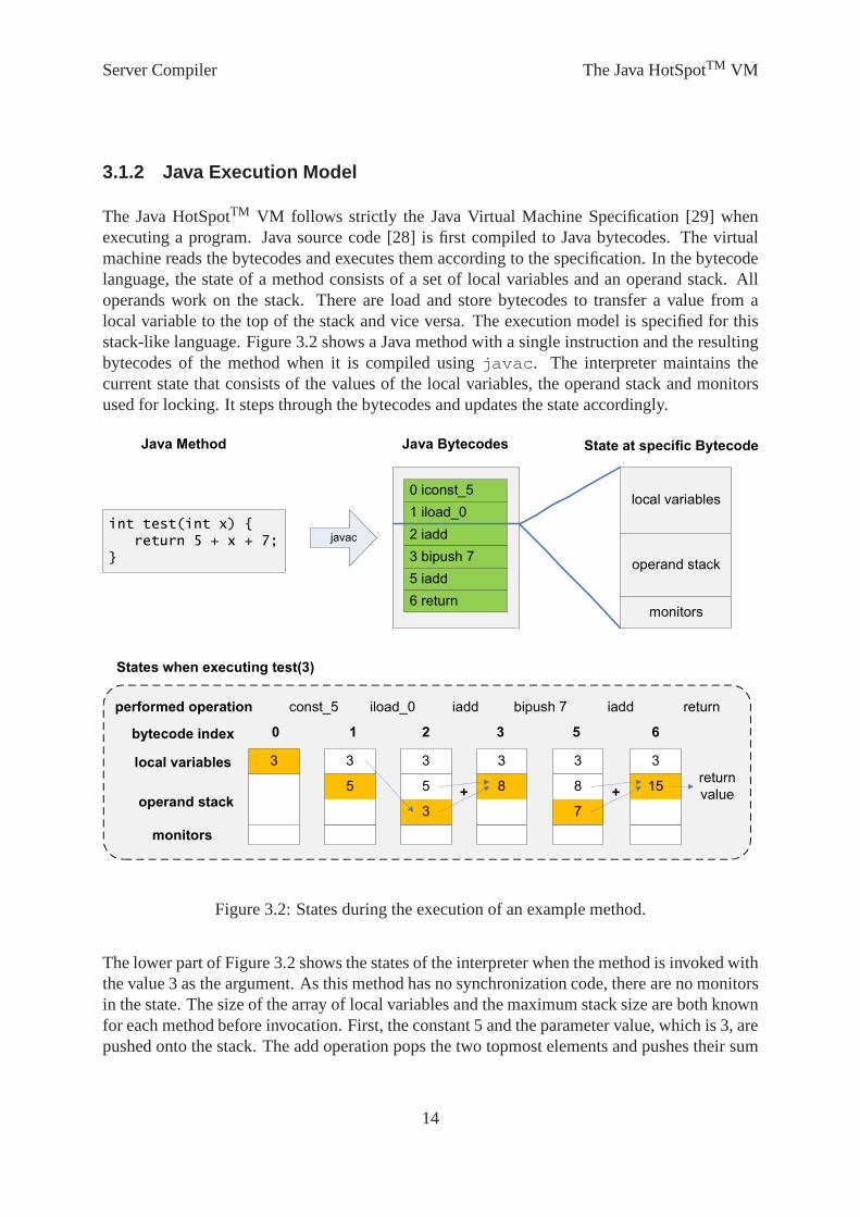
The Java HotSpotTM VM follows strictly the Java Virtual Machine Specification [29] whenexecuting a program. Java source code [28] is first compiled to Java bytecodes. The virtualmachine reads the bytecodes and executes them according to the specification. In the bytecodelanguage, the state of a method consists of a set of local variables and an operand stack. Alloperands work on the stack. There are load and store bytecodes to transfer a value from alocal variable to the top of the stack and vice versa. The execution model is specified for thisstack-like language. Figure 3.2 shows a Java method with a single instruction and the resultingbytecodes of the method when it is compiled usingjavac. The interpreter maintains thecurrent state that consists of the values of the local variables, the operand stack and monitorsused for locking. It steps through the bytecodes and updatesthe state accordingly.
local variables
operand stack
monitors
State at specific Bytecode Java Bytecodes
0 iconst_5
1 iload_0
2 iadd
3 bipush 7
5 iadd
6 return
Java Method
int test(int x) {
return 5 + x + 7;
}
javac
States when executing test(3)
3
0
3
1
3
2
3
3
3
5
3
6bytecode index
local variables
operand stack5 5
3
8 8
7
15+ +return
value
monitors
performed operation const_5 iload_0 iadd bipush 7 iadd return
Figure 3.2: States during the execution of an example method.
The lower part of Figure 3.2 shows the states of the interpreter when the method is invoked withthe value 3 as the argument. As this method has no synchronization code, there are no monitorsin the state. The size of the array of local variables and the maximum stack size are both knownfor each method before invocation. First, the constant 5 andthe parameter value, which is 3, arepushed onto the stack. The add operation pops the two topmostelements and pushes their sum
14

Server Compiler Architecture of the Server Compiler
onto the stack. Afterwards, the constant 7 is pushed and again an add operation is performed.The returned result is the topmost stack element at the end ofthe execution of the method.
When the interpreter is given a correct state for a bytecode,it can continue the execution inthe middle of a method. This property is used by deoptimization. The registers and memorylocations from which the current state can be reconstructedare tracked by the compiler. When itwants to deoptimize at a specific location, it inserts the statements that construct the interpreterstate and call the interpreter. Internally, the server compiler works with a program dependencegraph instead of stack operations. While constructing the graph, the compilers maintain whichnodes correspond to the current value of the local variablesand the elements on the stack.
3.2 Architecture of the Server Compiler
Figure 3.3 shows the steps applied by the server compiler when processing a method. Thecompiler starts with an empty graph and adds nodes to it whileparsing the bytecodes. Whenevera node is added, it performs locally the optimizations identity, global value numbering [4] andconstant folding (see Section 3.4). Afterwards it cleans upthe graph by properly building themethod exits and performing dead code elimination.
The next steps are global optimizations applied to the graph. They are not mandatory and canbe skipped by the compiler. After applying an iterative global value numbering algorithm, theideal loop step is performed at most three times. The ideal loop phase is capable of doingloop peeling, loop unrolling, and iteration splitting (forrange check elimination). When majorprogress is made running the ideal loop phase, it is run again, otherwise the compiler continueswith the next step. Conditional constant propagation is an optimization that combines simpleconstant propagation with the ability to removeif statements when the result of their conditionis constant. Then iterative global value numbering and several ideal loop phases are performedagain.
The ideal graph is then converted to the more machine specificMachNode graph (see Sec-tion 3.5). Basic blocks are built from the control dependencies. For every node, the latest andearliest possible scheduling is computed satisfying the property that it must be scheduled afterall its predecessors and before all its successors. The chosen location of a node should be lateto avoid unnecessary computations that are never used, but it should be outside of loops when-ever possible. A graph coloring register allocation (see Section 3.6) is performed. After somepeephole optimizations, the final machine code is generatedfrom theMachNode graph.
15

Server Compiler Ideal Graph
Once per BytecodeBuilding Ideal Graph
Code GenerationOptimizations
Iterative Global Value Numbering
Parsing Bytecodes Constant Folding
Identity
Global Value Numbering
Build Exits
Dead Code Elimination
Ideal Loop
Conditional Constant Propagation
Iterative Global Value Numbering
Ideal Loop
Generate MachNode Graph
Build Control Flow Graph
Register Allocation
Peephole Optimizations
Output Machine Code
Figure 3.3: Architecture of the Java HotSpotTM server compiler of Sun Microsystems.
3.3 Ideal Graph
The representation of the program in the compiler highly affects the complexity and effective-ness of applied optimizations. A common representation of aprogram is acontrol flow graph.The source code is a flat sequential structure with an exactlydefined order of the instructions.An instruction is defined by an operator and operands that arepreviously defined instructions.The control flow graph groups instructions that are guaranteed to be executed consecutively intobasic blocks.At the end of every basic block there is a conditional branch or a jump. A basicblock is connected with its predecessors and successors regarding control flow.
The Java HotSpotTM server compiler uses a control flow representation in the later stages ofcompilation. For most of its optimizations, however, it uses a data structure that combinescontrol flow and data dependencies. This graph data structure is calledideal graph. The in-structions are not ordered, but form a graph where the edges denote either definition-use datadependencies or control dependencies. By handling controland data dependence more uni-form, some of the optimization steps, especially those involving code motion, are less complex.Implementation details of the graph are described in [8].
16

Server Compiler Ideal Graph
The program dependence graph in the server compiler is a graph data structure with lightweightedges. An edge in the graph is only represented by a C++ pointer to another node. A node is aninstance of a subclass ofNode and has an array ofNode pointers that specifies the input edges.The advantage of this representation is that changing an input edge of a node is fast.
3.3.1 Data Dependence
Figure 3.4 shows a part of the program dependence graph generated by the compiler whenprocessing the expressionp*100+1wherep denotes a parameter of the current method. Nodesare represented by filled rectangles with the type of the nodeand some additional informationin them. Edges are drawn without arrows, but they always start at the bottom side of a nodeand end at the top side of a node. The layout arranges the nodesso that most edges are goingdownwards. Every node has a fixed number of input slots that can optionally be used as an endpoint of an input edge. There are some special nodes that allow an arbitrary number of inputedges. These additional edges are always stored after the obligatory input slots.
Figure 3.4: Program dependence graph when processingp*100+1.
The operations are represented in the graph by nodes that areconnected with the operands. TheMulI and theAndI node both take two integer operands. They have three available slots, butthe first one is not used in this example. Parameters are accessible via theParm node, theadditional informationParm0: int indicates that it is the parameter with index 0 and that itis of typeint. The constants 100 and 1 are also represented as nodes.
3.3.2 Empty Method
Figure 3.5 shows the graph of an empty method. Every graph hasaRoot node and this nodeis always connected to theStart node. To make traversing the graph simpler, nodes at whichthe method is exited have an outgoing edge to theRoot node. A node produces exactly oneoutgoing value, so the outgoing edges have no particular order. Projection nodes likeParm areused to model nodes that produce tuples. TheStart node produces the following values:
17

Server Compiler Ideal Graph
Control: The control flow is modeled as edges just like data dependencies. The semantic ishowever different. The graph formed when all non-control edges are removed can beviewed as a petri net. When the method is executed, the control token passes along thecontrol edges from node to node. AnIf node has two projection nodes as successors.The control token uses one of the two ways.
I_O: This type exists for historical reasons. It is used to serialize certain instructions.
Memory: To serialize memory stores that could interfere with each other, a type to expressmemory dependencies is used.
Frame Pointer and Return Address: Projection nodes that represent the value of the framepointer and the return address. They are produced by theStart node and are mostlyhidden to simplify the graph.
Figure 3.5: Graph when processing an empty method.
3.3.3 Phi and Region Nodes
The ideal graph is instatic single assignment(SSA) form [9]. This means that a value isassigned only once to a symbol at its definition and is never changed. To model conditionalassignment, e.g. if a variable gets assigned different values in different control flow paths,Phinodes are necessary. They merge values from different control flows. In the ideal graph theyare always connected toRegion nodes, which merge the control flow.Region nodes areusually inserted at the end ofif statements or at the loop header. The first input of aPhi nodeis always connected to its correspondingRegion node. The other inputs specify the valuesselected for each control flow going into theRegion node.
18

Server Compiler Ideal Graph
int test(int x) {
if(x == 1) {
return 5;
} else {
return 6;
}
}
Figure 3.6: Graph when processing anif statement.
Figure 3.6 shows the Java source code and the graph representation of a method containing anif statement. TheCmpI node compares the parameter and the constant 1. TheBool node isrelated to theCmpI node and specifies the compare operator, in this case the unequal operatoris used. TheIf node splits control flow into a true and a false path. These twopaths are mergedby theRegion node. The value of thePhi node is in dependence of the taken control floweither the constant 5 or the constant 6. The small circle above the first input of theRegionnode indicates that this first input is connected to the region node itself. EveryRegion node isconnected to itself, which makes the block finding algorithms easier. The order of the inputs oftheRegion andPhi nodes is essential. APhi node gets the value of its nth input when thecontrol path corresponding to the nth input of theRegion node is taken.
19
Server Compiler Ideal Graph
3.3.4 Safepoint Nodes
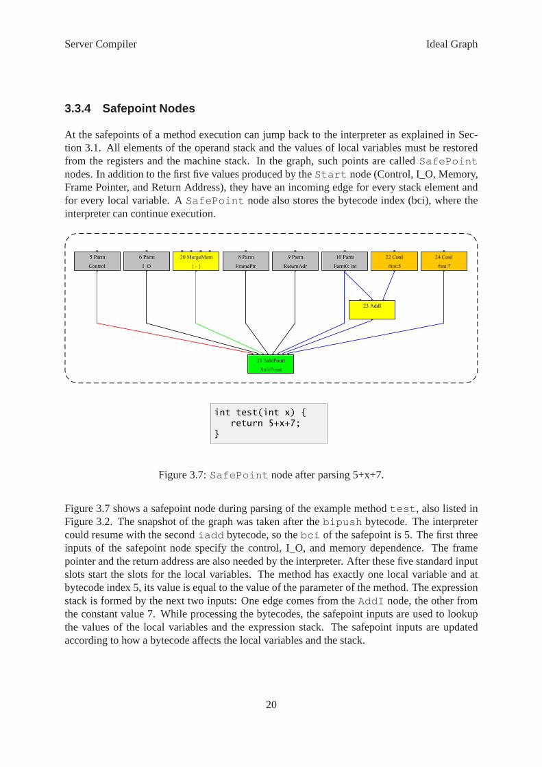
At the safepoints of a method execution can jump back to the interpreter as explained in Sec-tion 3.1. All elements of the operand stack and the values of local variables must be restoredfrom the registers and the machine stack. In the graph, such points are calledSafePointnodes. In addition to the first five values produced by theStart node (Control, I_O, Memory,Frame Pointer, and Return Address), they have an incoming edge for every stack element andfor every local variable. ASafePoint node also stores the bytecode index (bci), where theinterpreter can continue execution.
int test(int x) {
return 5+x+7;
}
Figure 3.7:SafePoint node after parsing 5+x+7.
Figure 3.7 shows a safepoint node during parsing of the example methodtest, also listed inFigure 3.2. The snapshot of the graph was taken after thebipush bytecode. The interpretercould resume with the secondiadd bytecode, so thebci of the safepoint is 5. The first threeinputs of the safepoint node specify the control, I_O, and memory dependence. The framepointer and the return address are also needed by the interpreter. After these five standard inputslots start the slots for the local variables. The method hasexactly one local variable and atbytecode index 5, its value is equal to the value of the parameter of the method. The expressionstack is formed by the next two inputs: One edge comes from theAddI node, the other fromthe constant value 7. While processing the bytecodes, the safepoint inputs are used to lookupthe values of the local variables and the expression stack. The safepoint inputs are updatedaccording to how a bytecode affects the local variables and the stack.
20

Server Compiler Optimizations
3.4 Optimizations
While building the graph by processing the bytecodes, localoptimizations are applied. Afteradding a node to the graph the compiler checks whether the newly added node can somehowbe replaced by another node that does the same computation ina cheaper way. There arethree such optimizations implemented: Identity optimization, constant folding, and global valuenumbering. The program dependence graph data structure allows some of the optimizationsrun in parallel benefiting from each other [6][7]. The following three subsections give smallexamples for each of them. The fourth subsection presents anexample of an optimizationapplied globally after parsing.
3.4.1 Identity Optimization
The identity optimization searches for nodes that compute that same result. In contrast to globalvalue numbering, it searches also for nodes that are different, but produce the same output.Figure 3.8 shows how the expressionx+0 is processed by the server compiler. First, the fullexpression including theAddI and theConI node are generated (left side). Now the identityoptimization finds out that theParm node produces always the same result as the newly createdAddI node and uses only theParm node further on. After parsing all bytecodes, the compilerperforms a dead code elimination: It deletes theAddI node and theConI node. The resultinggraph is shown on the right side.
Figure 3.8: Identity optimization:(x+0) is transformed tox.
21

Server Compiler Optimizations
3.4.2 Constant Folding
Arithmetic operations on constants are performed at compile time and the result is representedby a constant node. In Figure 3.9 the graph for the expression5+p+7 is shown. The first addoperation5+p is modeled as anAddI node, but it is immediately transformed to the expressionp+5, as the convention that the constant part is always the last input simplifies constant folding.After the compiler has generated the nodes for the second addoperation, the constant foldingalgorithm identifies a simplification possibility and the whole expression is replaced byp+12.The algorithm looks for the pattern that the second input of the add operation is a constant andthe first input is anAddI node, which has a constant input too. Dead code elimination removesthe unnecessary two constant nodes and theAddI node.
Figure 3.9: Constant folding:(5+p+7) is transformed to(p+12).
3.4.3 Global Value Numbering
Global value numbering is an optimization similar to the identity optimization. It searches fornodes that are equal to the currently inserted nodes. Equality means that the nodes themselvesand also all of their inputs are equal. In this case, only one of them is needed and the other onegets deleted by dead code elimination. A node has a hash valuefor fast equality testing. It isbased on its properties and the C++ memory addresses of its inputs.
Figure 3.10 shows the graph produced when compiling the statement(x+1)*(x+1). The leftgraph is a snapshot taken after the processing of(x+1). In the middle the second(x+1) isrepresented by theAddI and theConI node. As the hashcode of the twoAddI nodes is thesame, the oldAddI node is connected a second time to the safepoint node insteadof the newlycreatedAddI node. So the followingMultI node gets a connection to the firstAddI nodein both slots. After dead code elimination the compiler deletes the secondAddI node. Theresulting graph is shown on the right side.
22

Server Compiler Optimizations
Figure 3.10: Global value numbering:(x+1)*(x+1) is transformed to(x+1)2.
3.4.4 Loop Transformations
The server compiler performs a large number of global optimizations after parsing. They canbe divided into three main categories: Iterative global value numbering, conditional constantpropagation, and loop transformations. As presenting all of them would go beyond the scope ofthis thesis, only the step to identify counted loops is described in this section.
The identification of loops brings advantages for array bounds check elimination and is nec-essary for loop unrolling and loop peeling. After parsing the bytecodes, a loop is representedby a control flow cycle involvingRegion nodes. The first task is to find regular loops withinthe graph and identifyRegion nodes that representloop headers, i.e. nodes that the controltoken must always pass when entering the loop. A loop header is represented by aLoop node,which replaces theRegion node. When the input bytecodes were created by compiling Javacode, then there exist only loops with one entry. There are however no such restrictions onthe bytecodes. As loops with more than one entry are a rare case and handling them would becomplicated, the server compiler does not optimize such loops.
A common loop pattern is represented by a loop variable starting at a specific value and goingconstant steps up to an upper bound. After reaching the bound, the loop is exited. Somelanguages like FORTRAN have language constructs for this kind of loops, but in Java thismust be coded using a local variable and manually inserted increments and conditions. Thereare special optimizations for such loops, so the server compiler identifies the loop pattern andconverts it to a construct with aCountedLoop node and aCountedLoopEnd (CLE) node.Figure 3.11 shows the nodes that define a counted loop. They specify the beginning and end ofthe loop, as well as the loop variable and the increment per loop iteration.
23

Server Compiler MachNode Graph
Loop entry
Backedge
Loop exit
Initial loop variable value
Stride value
Figure 3.11: Nodes that define a counted loop.
3.5 MachNode Graph
After all global optimizations are applied, the ideal graphis still in a machine-independent form.The next step is converting the graph to a more machine-near form. The resulting nodes are laterscheduled and directly converted to machine code. Bottom-up rewrite systems [24] can be usedfor the optimal selection of machine instructions when producing machine code from expressiontrees. The server compiler selects subtrees out of the idealgraph and converts them one by one.It selects specific nodes as root nodes and transforms their related tree using tree selection rules.Some nodes likePhi nodes are marked asdontcare and have no corresponding nodes inthe new graph. Other instructions are marked asshared, which means that they must notbe shared among subtrees. Code for instructions that are part of more than one subtree isduplicated. The result of the root node of a tree is always placed in a register so it can be reusedwithout recomputation.
24

Server Compiler MachNode Graph
Figure 3.12: Matching and register allocation example.
Each tree is converted using a deterministic finite automata. There exist architecture descriptionfiles for i486, AMD64, andSparc that describe the available instructions and their costs.Listing 3.1 shows schematically an extract of thei486 architecture description file. The linestarting withmatch specifies the tree pattern that can be converted by this rule.A rule has anassociated estimated cost. The compiler matches a tree suchthat the total cost of applied rules
25

Server Compiler Register Allocation
is minimal. The file also contains additional properties of the rules including for example theresulting machine code. The first rule converts aCmpI node with a register and an immediateoperand to acompI_eReg_imm node. The second rule can convert aCMoveI node with twoBinary nodes as predecessors to a singlecmovI_reg node.
Listing 3.1 Architecture description file extract.// Signed compare instructioninstruct compI_eReg_imm: flags cr, register op1, immediate op2match: Set cr (CmpI op1 op2)opcode: 0x81,0x07
// Conditional moveinstruct cmovI_reg: register dst, register src, flags cr, operator copmatch: Set dst (CMoveI (Binary cop cr) (Binary dst src))ins_cost: 200opcode: 0x0F,0x40
Figure 3.12 shows how the graph for the example method presented in Figure 3.6 is convertedto a machine-specific form. During global optimizations, the compiler replaces theIf and thePhi node with aCMoveI node (see top-left). For the rules to match correctly some constructsmust be changed. In this case, the twoBinary nodes are inserted and form new inputs of theCMoveI node (see top-right). The matcher identifies that the two rules defined in
Listing 3.1 can be applied. The twoConI nodes representing the values 5 and 6 are convertedto loadConI nodes. The node for constant 1 is no longer necessary, because the informationthatcompI_eReg_imm should compare the input with 1 is modeled as a parameter. ThenodecmovI_reg is created according to the second rule. The bottom-left graph shows the result ofthe matching process.
After the construction of theMachNode graph, the compiler builds the control flow graphconsisting of basic blocks and schedules the nodes. Then theregister allocator selects machineregisters for the nodes (see bottom-right graph).
3.6 Register Allocation
Register allocation selects machine registers to hold values that must be stored between calcu-lations. If there are not enough registers available to holdall values, they must be temporarilystored in the main memory, which is an expensive operation called spilling. The goal is to haveas less spillings as possible when executing a method. Thelife rangeof a value is the rangebetween its production and its last usage. Two values can be stored in the same register if theirlife ranges do not intersect. If the life ranges intersect, then at some time both of them must bestored, so it is impossible to store both values in the same register.
26

Server Compiler Register Allocation
The server compiler uses a graph coloring register allocator [5][3]. First it builds aninterferencegraph, which is a graph with the values as nodes and an undirected connection between twonodes if their life ranges intersect. A coloring of a graph isan assignment of a color to eachnode of the graph with the restriction that two directly connected nodes must not have the samecolor. When the available registers are viewed as the colors, then a valid coloring the graph isa valid register allocation. Two values that have intersecting life ranges are directly connectedin the interference graph and get therefore different registers assigned. When it is not possibleto color the graph, then spilling a value is unavoidable. Thelife range of the value is splitted:one life range between its production and the storage to memory, another life range betweenits loading from memory and its last usage. Now the interference graph has a better chance ofbeing successfully colored as most likely some of the connections of the original life range donot exist in one of the two shorter new life range intervals..
First, the algorithm to color a graph withn colors selects nodes with less thann neighbors.Obtaining a correct color for such a node is trivial when the rest of the graph is successfullycolored. The node gets the color that is not used by any of its neighbors and as there are max-imal n-1 neighbors, such a color always exists. Such easily colorable nodes are consecutivelyremoved from the graph. If at some point there is no such node,then the graph is not colorable.The server compiler iteratively inserts spilling code until a valid coloring is found.
The register allocation by graph coloring is expensive for large methods. The client compileruses a linear scan register allocator [31] instead of a graphcoloring algorithm.
27

Chapter 4
User Guide
This user guide introduces the most important functionalities of the Java HotSpotTM servercompiler visualization tool. The tool consists of a Java application, which is used to displayand analyze the graphs, and an instrumentation of the Java HotSpotTM server compiler thatgenerates the data. Figure 4.1 shows the global architecture. There are two ways to transferthe data from the server compiler to the Java application, either via intermediate XML files ordirectly via a network stream. The Java application consists of several window components thatare explained in this user guide.
Server Compiler
XML file
Network Stream
Outline Window Properties Window Filter Window
Editor Windows
Java Application
Instrumentation
Figure 4.1: Architectural overview.
28

User Guide Generating Data
4.1 Generating Data
A special debug version of the Java HotSpotTM server compiler is needed for generating data.It has an additional command line option-XX:PrintIdealGraphLevel=l that specifieshow detailed the compiled methods should be recorded, i.e. how many snapshots of the graphshould be taken during compilation. There are four different levels:
Level 0: This is the default value and stands for disabling tracing atall.
Level 1: At this level only three states per method of the graph are traced: one state immedi-ately after parsing, one state after the global optimizations have been applied, and onestate at the end of compilation before machine code is generated.
Level 2: This level includes intermediate steps for the global optimizations: iterative globalvalue numbering, loop transformations, and conditional constant propagation. The num-ber of graphs depends on the number of applied optimization cycles. Additionally, thestate of the graph is traced before it is converted to aMachNode graph and once beforeregister allocation.
Level 3: The third level is detailed: After each parsed bytecode, thecompiler traces a graphstate, and the loop transformations are dumped with more intermediate steps.
With increasing level, the necessary storage space and compile time overhead increases too, sothe lowest needed level should be used.
At startup, the server compiler tries to open a network connection to the Java visualization ap-plication. The two options-XX:PrintIdealGraphAddress=ip specifies the networkaddress and-XX:PrintIdealGraphPort=p the port. The default values are "127.0.0.1",i.e. the local computer, and port 4444. If opening of the connection succeeds, the data is im-mediately sent to the tool. Otherwise, the data is saved to a file calledoutput_1.xml. Withmultiple compiler threads the second thread saves its data to output_2.xml and so on.
All compiled methods are recorded. By default the Java HotSpotTM VM decides based on theinvocation count and the number of loop iterations when it schedules a method for compilation.The flag-Xcomp completely disables the interpreter, so all methods get compiled before theirfirst invocation. Using this flag however means that a large number of methods get compiled.The option-XX:CompileOnly=name can be used to restrict compilation to a certain classor method.
The currently loaded methods of the application are available in the Outline Window. XML datafiles can be loaded using theFile->Open menu item. When the network communication isin use, the transferred methods appear automatically. In the top section of the Outline Window,listening on a port for data can be enabled and disabled with acheckbox. Additionally, a filtercan be specified to reduce the number of methods that should betraced. The server compilersends only methods to the Java application if their name contains the string specified in thetextbox next to the checkbox.
29

User Guide Viewing the Graph
The methods appear with a folder icon and the available snapshots for a method are childelements . Double clicking on a snapshot opens a new editor window in the center anddisplays the graph.
4.2 Viewing the Graph
The viewed graph consists of nodes with input and output slots and edges that connect two slots.The input slots are always drawn at the top of a node, the output slots at the bottom. When anode is selected using the left mouse button, its key-value pairs are shown in the PropertiesWindow. This functionality is also available for all items in the Outline Window. The text thatappears inside the nodes is an extract of their property values and can be customized in the pref-erences dialog. Figure 4.2 shows the editor window of an example graph and the correspondingProperties and ControlFlow Window.
Key-Value
Pairs
Backward
Edge
Search
Panel
Selected
NodeControl Flow
Figure 4.2: Viewing a graph using the Java application.
Right-clicking on an edge shows a context menu with its source and destination nodes. This isespecially useful for edges that are only partially visible. When an edge would be so long that it
30
User Guide Navigating within the Graph
disturbs the drawing, it is cut and only its beginning and ending is drawn. By default, the nodesare drawn grouped into clusters. This can be turned off and onusing a toolbar button .
Rolling the mouse wheel zooms in and out, there are also toolbar buttons available for thispurpose . The currently shown extract of the graph is changed by holding the middlemouse button pressed and dragging around. A detailed description of how to navigate throughthe graph is given in the next section. The current graph can be exported to an SVG file usingtheFile->Export menu item.
When a graph is currently opened, the difference to a second graph can be calculated: Right-clicking on another graph and selecting the optionDifference to current graphopens a new window with an approximation of a difference between the two graphs.
4.3 Navigating within the Graph
As in most cases only a particular part of a graph is of interest, navigation possibilities aremandatory. When a graph is opened for the first time, all nodesare visible and the root node isshown horizontally centered on the screen. Selected nodes can be hidden from the view usingthe context menu or a toolbar button . There is a button to show again all nodes. In thecontext menu of a node, two submenus allow to navigate to one of its immediate predecessorsor successors.
Nodes that are not marked as fully visible can be either semi-transparent or invisible: Not fullyvisible nodes are semi-transparent when they are connectedto a node that is fully visible, oth-erwise they are invisible. When such semi-transparent nodes are double clicked, they becomefully visible. On the other hand, fully visible nodes becomesemi-transparent or invisible whenthey are double clicked. This allows fast expanding and shrinking of the current set of visiblenodes without using the context menu. There is one exceptionof the double click semantics:When all nodes are fully visible, then double clicking on a node does not hide this node, buthides all other nodes of the graph.
So the standard use when analyzing a specific node is to first search for the node in the fullgraph. Then show only this node by double clicking it and afterwards expand the predecessorsand successors of the node as needed. When the selection of the target node set is done, thesemi-transparent nodes are more disturbing than helpful inmost cases. Therefore they can becompletely hidden using the toolbar button .
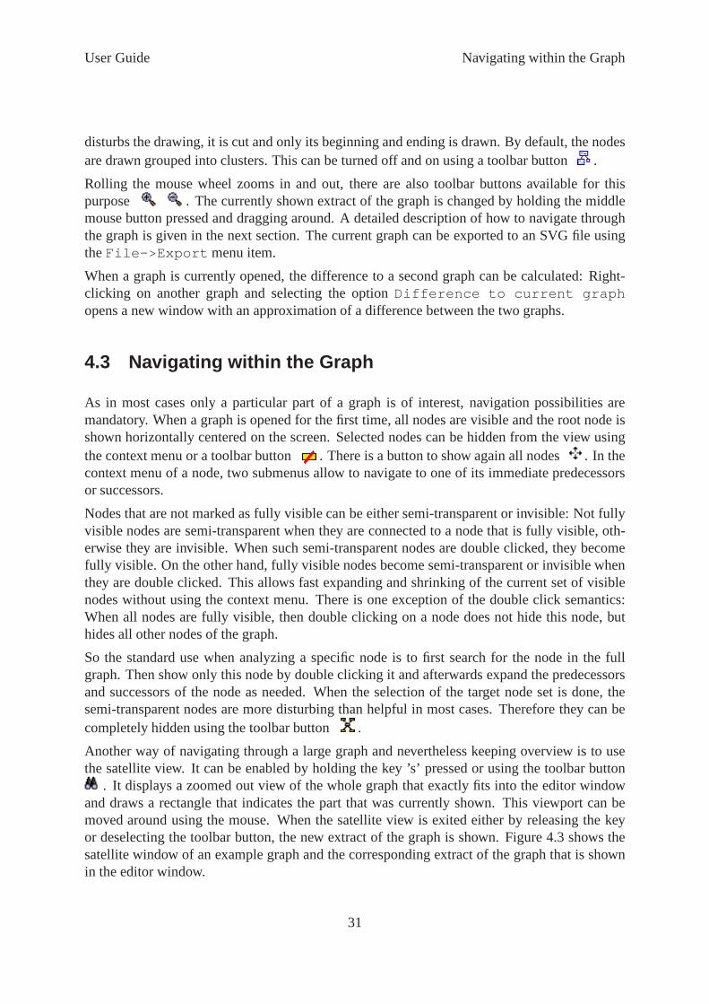
Another way of navigating through a large graph and nevertheless keeping overview is to usethe satellite view. It can be enabled by holding the key ’s’ pressed or using the toolbar button
. It displays a zoomed out view of the whole graph that exactlyfits into the editor windowand draws a rectangle that indicates the part that was currently shown. This viewport can bemoved around using the mouse. When the satellite view is exited either by releasing the keyor deselecting the toolbar button, the new extract of the graph is shown. Figure 4.3 shows thesatellite window of an example graph and the corresponding extract of the graph that is shownin the editor window.
31

User Guide Control Flow Window
Satellite ViewCurrent Extract
press key “s”
release key “s”
Figure 4.3: The satellite view gives an overview of a graph.
4.4 Control Flow Window
To increase the overview in large methods, an approximationof the control flow graph is avail-able. Every node is assigned abasic block, i.e. a set of instructions that are executed consecu-tively without any branches. The Control Flow Window shows agraph with a node for everyblock that is connected to the block’s predecessors and successors. Note that this is only anapproximation as the real control flow information is only available in a late stage during com-pilation. Every node is put in the latest possible block fulfilling the condition that it must beevaluated before all its successors. Selecting a block selects all nodes that are assigned to thisblock in the full graph and centers them in the view. Invisible nodes of the block get automati-cally visible.
4.5 Filters
The graph coming from the server compiler does not contain any display information. The onlyadditional information available beside the graph description are key-value pairs for the nodesof the graph. Filters change the representation of the graphbased on node properties. There
32

User Guide Filters
are filters for changing the color of nodes and edges, for removing nodes and also two specialfilters for combining and splitting nodes.
In the Filter Window, all currently available filters are listed in their processing order. Filterscan be activated and deactivated using the checkbox left to their name. The toolbar buttons onthe right allow adding , removing , and moving filters . The current set ofselected filters can be saved as a profile and is then recallable using the combobox on theleft.
The following list explains the standard filters that are available when first installing the tool.They all use selection rules based on key-value pairs and canbe customized.
Basic Coloring: Color filter that should be enabled by default. It sets a standard color andspecial colors for control flow specific nodes.
Matcher Flags Coloring: Before converting the ideal graph to aMachNode graph, the twoflagsis_shared andis_dontcare are calculated. This filter visualizes the flagswhen their value is available.
Register Coloring: Colors the nodes according to the selected register. The register allocatorinformation is available at a late stage during compilation.
Extended Coloring: Gives a color to constant nodes, projection nodes, and nodesthat have abci property, i.e. nodes that are safepoints.
Line Coloring: Colors the connections according to the type of the source node. Differentiatesbetween integer values, control flow, memory dependencies,tuple values, and the specialtypebottom.
Difference Coloring: In a difference graph all nodes have a state expressed as a property thatcan be either same, changed, new or deleted. According to this state, the filter sets a nodecolor. When the nodes do not have a state property, the graph remains unchanged.
Only Control Flow: This filter is useful when the full graph is too complex and oneonly wantsto focus on the control flow. It removes all nodes that do not produce a control flow valueand are not immediate successors of a node that produces a control flow value.
Remove FramePtr, I_O, and ReturnAddress: Removes the three nodes FramePtr, I_O, andReturnAddress from the graph as they normally are not of interest and disturb the view ofthe graph. They are connected to all safepoint nodes.
Remove Memory: Removes any node that produces a memory dependence as its value.
Remove Root Inputs: Every possible end of a method has a backward edge going to therootnode. So for large graphs the number of inputs into the root node can be high, whichdisturbs the drawing. Therefore this option should be enabled as the root inputs are notof interest in most cases.
33

User Guide Filters
Remove Safepoint Inputs: The inputs of a safepoint specify the values of the expression stackand local variables at the safepoint’s bci. This is interesting when the graph is built fromthe bytecodes, but not very important afterwards. Removingthe inputs improves theoverview and the drawing performance.
Combine: When a node produces more than one output value, it produces atuple and thespecific values must be selected using projection nodes. This filter combines such a nodewith all its projection nodes and creates a single node with multiple output slots.
Split: Constants are shared among all nodes. So when a constant is used multiple times, allusages refer to a single node representing the constant. This is reasonable to save memorycapacity but is impractical for displaying the graph. This filter removes constant nodesand writes their value directly to all slots where they were used.
Filters are written in JavaScript using Java objects and shortcut functions. Double clicking ona filter opens a dialog that allows editing its name and its code. Filters are programmed basedon selection rules applied to the graph. There exist some predefined functions that cover mostfiltering tasks. They are listed in the following table:
colorize(name, regexp, color)
Colors all nodes whose propertynamematches the regular expressionregexp.Predefined color variables are:black,blue, cyan, darkGray, gray, green,lightGray, magenta, orange, pink,red, white, andyellow.
remove(name, regexp)Removes the matching nodes from thegraph.
removeInputs(name, regexp,start, end)
Removes all inputs from the matchingnodes from the indexstart to the indexend.
split(name, regexp) Splits the matching nodes.
regexp stands for a string representing the regular expression that the value of the propertywith the specified name must fulfill. The syntax corresponds to the standard Java regular ex-pression syntax used by the classes in thejava.util.regex package. Amongst others, thefollowing rules are defined: "." stands for any character, "*" means that the preceding elementis repeated zero or more times, and "|" expresses alternatives.
Figure 4.4 shows each of the predefined functions applied to an example graph. The plain graphwithout any filters applied is displayed top left. Then the graph is colored using thecolorizefunction and regular expressions. Afterwards thePhi node is removed. The functionsplitremoves theConI node from the graph and displays the short name for the node atevery use.So "0" is drawn at the third input of theCmpI node. The last applied step removes the secondinput of theStart node.
34

User Guide Filters
The search panel in the toolbar of the center window works in asimilar way to a filter. Aproperty name can be selected in the combobox, and a regular expression that this property ofthe target nodes must fulfill can be entered in the textfield. After pressing enter in the textfieldor the search toolbar button , all matching nodes are selected.
Start graph colorize(“name”, “.*I”, green)
remove(“idx”, “38”) split(“name”, “Con.*”) removeInputs(“idx”, “3”, 1, 1)
colorize(“name”, “Root”, orange)
Figure 4.4: Four functions applied to an example graph.
35

User Guide Bytecode Window
4.6 Bytecode Window
The Bytecode Window shows the Java bytecodes of the method from which the currentlyopened graph was generated. Bytecodes that are referenced from nodes through the bci prop-erty are shown with a special icon. Double clicking on such a bytecode will select all nodes thathave a reference to it. These are mainly safepoint nodes.
The server compiler inlines small methods to avoid the overhead of calling them. The bytecodesof inlined methods are shown as child elements of a node beneath the bytecode that wouldinvoke the method. Figure 4.5 shows the bytecode view for an example method. The bytecodewith the index 3 is a call to another method, which the server compiler decided to inline. Thebytecodes of the inlined method are all shown in the sublist.There are two safepoint nodes inthe graph that reference the bytecode indices 13 and 25 of theinlined method. Therefore, thosebytecodes have a special icon and by double clicking on them, the corresponding nodes inthe graph are selected.
Inlined Method
Connected
with Nodes
Figure 4.5: Bytecode Window showing the Java bytecodes in tree-form.
36

Chapter 5
Visulializer Architecture
In this chapter, the architecture of the visualization application that is based on the NetBeansplatform is explained. Additionally, it contains a description of the algorithm for finding the dif-ferences between two graphs. The layout algorithms and the code added to the server compilerare presented in two subsequent chapters.
5.1 Module Structure
The NetBeans application is split into several modules represented by NetBeans projects. Fora discussion of modular programming see Section 2.3. Figure5.1 shows the modules and theirdependencies. Transitive dependencies are omitted for simplicity. Two modules represent thirdparty libraries: RhinoScripting for the execution of JavaScript code and BatikSVG for the exportof SVG files. There are three top-level modules: Bytecodes, ControlFlow, and Coordinator.Here is a list of all modules in alphabetical order:
BatikSVG: The Batik SVG Toolkit is part of the Apache XML Graphics Project. SVG standsfor Scalable Vector Graphics and is a vector-based standardized graphics format. TheBatik SVG library allows to create a JavaGraphics object that writes into an SVG fileinstead of painting on the screen. The visualization tool uses this functionality to exportthe currently selected graph into an SVG file.
Bytecodes: A top-level module that is responsible for the bytecode viewof the method of thecurrent active graph. It listens to the lookup of the window with focus and displays thetree of bytecodes of the current graph’s method.
ControlFlow: Contributes the control flow view of the currently active graph and listens to thelookup of the current active window similar to the Bytecodesmodule. It is also a top-level module and uses the NetBeans visual library for displaying the control flow graph.It forwards the changes of the block selection to the active graph editor window.
37

Visulializer Architecture Module Structure
BatikSVG
Bytecodes
ControlFlow
RhinoScripting
Coordinator
Data
Difference Filter
Graph
Layout
HierarchicalLayout Settings
Util
View
Top-Level Modules
Third
-Party Librarie
s
Figure 5.1: Dependencies of the NetBeans modules.
Coordinator: Top-level module that contains the code for the outline and the filter window.All predefined filters are defined in this module. It is responsible for opening new grapheditors in the center area. The task of actually creating thewindow and displaying thegraph is forwarded to the View module.
Data: Contains the data model used to transfer data between the server compiler and the tool.It parses the XML data coming from the server compiler and converts it to an internaldata structure. It uses a SAX XML parser. For a detailed description of the data modelsee Section 5.2.1.
Difference: Used to create a difference graph of two input graphs. It depends only on the Datamodule and the Util module. The difference algorithm is explained in Section 5.5.
Filter: Contains the filters that can be applied to the graph model andthe dialog to edit a filter.It depends on the Graph module and the RhinoScripting modulefor executing JavaScriptcode. Section 5.4 contains a description of the filter architecture.
Graph: The data model used internally for the graphically enrichedgraph. In comparison tothe data model defined in the Data module, it adds display information to the nodes andedges of the graph. For a detailed description see Section 5.2.2. Additionally, it containsthe graph selectors that are used by the filters and are explained in Section 5.4.
38

Visulializer Architecture Graph Models
Layout: Defines an API for layouting a graph which is explained in Section 5.2.3. It containsthe interface definitions for the nodes and edges of the graphand also an interface forclusters of nodes.
HierarchicalLayout: Actual implementation of a graph layouter as defined in the Layout mod-ule. It also contains a hierarchical layouter that can handle clustering. The layout algo-rithms are explained in Chapter 6.
RhinoScripting: Rhino is an open source implementation of a JavaScript engine and is part ofthe Mozilla project. It contains all features of JavaScript1.5. The visualization tool usesthe library to allow the user to write filters in JavaScript code.
Settings: Module that is responsible for loading and storing settingsthat should be persistent.It also contains the code for displaying the settings dialog.
Util: Contains some utility classes that are used by other modules. It contains the definitionsfor the properties mechanism described in Section 5.3.
View: Responsible for displaying the graph in a new editor window.It uses the NetBeansvisual library to render the graph. For a description of the visual library see Section 2.6.
5.2 Graph Models
The application uses three different models for the graph: The data modelfor the transfer ofthe data from the server compiler to the Java application, the display modelfor displaying andfiltering the graph, and thelayout modelfor layouting the graph. Working with different modelscomes with the cost of converting between them. The data model is converted to the displaymodel whenever a graph is opened in a new editor window. The layout model is a submodel ofthe display model, so no conversion is needed there. An advantage of using different models isthe avoidance of unused fields. For example, all fields containing display information such asthe color of the nodes would be undefined for all loaded graphsand would only get a meaningafter a graph is opened.
The application saves for every node of the display graph model the corresponding nodes in thedata model. When the graph of the display graph model is created for the first time, every newnode represents exactly one node of the data model. Through filters, however, a node of thedisplay model may represent several nodes of the data model.
Figure 5.2 shows the lifecycle of a graph and how it is converted between the models. Fortransmitting the data from the server compiler to the Java application and for storing it on thehard disk, an XML structure based on the data model is used. The Java application reads thedata and builds a memory representation of it. When a graph isopened in a new editor window,the data model representation of the graph is converted to a display model representation. Theapplication applies all activated filters on the graph and invokes the layout manager. The layout
39

Visulializer Architecture Graph Models
manager works on the layout model, which is a submodel of the display model. The editorwindows use the NetBeans visual library to show the display model representation of the graphon the screen. The following three sections describe the three models in detail.
Server Compiler
Outline Window
Layout ManagerXML file
Editor WindowApply Filter
Layout Model
Display ModelData Model
Figure 5.2: Lifecycle of the graph data.
5.2.1 XML File Structure
The data transferred from the server compiler to the visualization tool is represented in XML.The main advantage of using XML instead of a custom binary format is better changeability.When new XML elements are introduced, it is simple to maintain backward and forward com-patibility: On the one hand, the old application can read thenew XML data because it ignoresthe new elements. On the other hand, the new application can read the old XML data by ignor-ing the elements that are no longer valid. The main disadvantage of using XML is the higherstorage requirement compared to a binary format.
One of the goals when designing the data model was that it should be generally usable fordescribing directed graphs. This is an important design decision that opens the possibility thatthe visualization tool is used to analyze graph-like data structures of a completely differentapplication.
Another concept of the data model are properties based on key-value pairs. All descriptiveinformation about an entity is stored uniformly as a list of key-value pairs, instead of introducingXML attributes for the properties of Java methods, graphs, and nodes. This concept is usedthroughout the application and is explained more detailed in Section 5.3.
Figure 5.3 shows the XML elements and their relations. AgraphDocument is the top-levelelement and can containgroup child elements. The server compiler creates agroup ele-ment for every traced method. Agroup element has exactly onemethod child element thatdescribes the bytecodes and inlining of the method. Agroup element can have an arbitrarynumber ofgraph child elements that describe the traced states of the graph during compilationof the method. Agraph element has onenodes, oneedges, and onecontrolFlow childelement.
Concerning the nodes and edges, only the difference to the previous graph of the method issaved. Therefore, thenodes element can contain definitions of nodes asnode elements or
40

Visulializer Architecture Graph Models
removeNode elements, which state that a certain node of the previous graph is no longerpresent. A similar mechanism is used for the edges. Succeeding graphs of a method oftenhave similar nodes and edges. The number of equal nodes and edges depends on the number oftraced intermediate steps. Using a difference-based storage format highly reduces the necessarystorage space.
Every node has a unique identifier that is referenced from theedges and the control flow blocks.An edge is defined by the identifiers of its source and destination node and the index at whichthe edge ends at the destination node. ThecontrolFlow element contains the informationnecessary to cluster the nodes into blocks. For each block, its successor blocks and the nodesthat are related to that block are specified. The nodes are referenced via their unique id.
A method element contains two child elements: Theinlined element can have methodchild elements expressing inlining. The bytecodes of a method are stored in the textual formatthat is used to trace the bytecodes in the server compiler.
graphDocument
group
methodname
shortName graphname
inlined bytecodes
nodes edges controlFlow
node
id
removeNode
id
edgeindex
from
to
removeEdgeindex
from
to
blockname
dom
successors nodes
node
id
successor
name
properties
p
name
TEXT
TEXT
zero or one child
zero or more children
Figure 5.3: XML file structure.
The elementsgraphDocument, group, method, andnode can have apropertiessubelement that specifies key-value pairs via its child elements. The concept of properties isalso present in the data and the display model and is described in detail in Section 5.3.
The XML data is read using a parser that processes the elements while reading it. Readingfrom the network stream and reading from a file is treated in a uniform manner. The network
41

Visulializer Architecture Graph Models
communication between the server compiler and the visualization tool is interactive: After theserver compiler has sent agroup element and its properties, the client compiler writes thecharacter ’y’ if it wants to receive that group of graphs or ’n’ otherwise.
From the XML data, the data model memory representation is built. Figure 5.4 shows theclasses that represent the data model. The structure is similar to the XML structure. The nodesand edges are however no longer represented as the difference to the previous graph. The parserresolves this differences without any additional memory requirements by sharing theInput-Node objects. If a node does not change between two graphs of a method, then both graphscontain a memory pointer to that node.
GraphDocument
Group
InputBlock
InputBlockEdge
InputBytecode
InputMethodInputGraph
int from
int to
int index
InputEdge
int id
InputNode
*
*
*
*
2
**
*
0..1
PropertyObject
Properties API
Figure 5.4: Data module class diagram.
5.2.2 Display Model
The display model is similar to the data model, but contains display information for the nodesand edges of the graph. When a new editor window is opened, theapplication first creates anew display graph based on the data model graph. Then the filters are applied to the displaygraph and it is drawn on the screen.
There is a semantic difference concerning the graph betweenthe data and the display model: Inthe data model every node produces exactly one output, so it has exactly one output slot. Thisis due to the structure of the ideal graph in the server compiler. It is however possible that afilter combines several nodes into a single one with more thanone output slot. Therefore, thiscan be expressed in the display model, but cannot be expressed in the data model. Additionally,slots can have a shortcut that is displayed on the screen and ashort description that is shown asa tooltip.
Figure 5.5 shows the classes of the display model. The classDiagram corresponds to theclassInputGraph in the data model. A diagram can contain any number ofFigure objects.
42

Visulializer Architecture Graph Models
Figures can have any number of input and output slots. A connection is always between exactlyoneInputSlot object and oneOutputSlot object.
A figure has aSource object that points to one or moreInputNode objects of the data modelthat this figure represents. When the display model representation is constructed from the datamodel representation, everyFigure object has exactly oneSource object pointing to oneInputNode object. Filters may alter the graph and are responsible to keep the pointers to thedata model up-to-date. The filter that combines multipleFigure objects into a single one setsthe node pointers of theSource object of the new figure to the union of the node pointers oftheSource objects of the original figures.
Diagram
Figure
Slot
InputSlot OutputSlot
Source
InputGraph
InputNode
Data Model
Connection
*+
*
*
*
PropertyObject
Properties API
*
Figure 5.5: Display model class diagram.
5.2.3 Layout Model
The layout algorithm should be commonly usable, so a dependency on the display model shouldbe avoided. Converting the graph in the display model representation to another data structureis however computationally intensive. So the layout model is a submodel of the display model.This is implemented using the Java interface mechanism. Figure 5.6 shows a class diagram ofthe layout model.
In the layout model, a graph consists ofVertex objects that have a size and a position.Portobjects are assigned to aVertex object and have a position relative to theVertex object.A Link object represents an edge between twoPort objects. EachLink object has a list ofpoints in which the first and last are the start and end points of the edge. The other points areinterpolation points. The valuenull in the point list is valid and means that the edge shouldbe cut off at the previous point and resumed at the next point in the list.
43

Visulializer Architecture Graph Models
There is an additional aspect in the layout model that is relevant to layout algorithms that allowclustering of nodes. Each vertex is assigned to aCluster object. ACluster object itselfcan have a parentCluster object and preceding and succeedingCluster objects.
LayoutGraph is a concrete class that represents a layout graph consisting of Link objects.The Port objects andVertex objects are implicit defined by theLink objects as uncon-nected vertices are not interesting for layouting. ALayoutManager is capable of layoutingthe graph by setting the positions of theVertex objects, the point lists of theLink objectsand the bounds of theCluster objects.
TheFigure class of the display model implements theVertex interface. TheSlot classimplements thePort interface and theConnection class implements theLink interface.The cluster information is only available in the data model and is not converted to the displaymodel. The block of aFigure object is retrieved by getting the block of theInputNodeobjects the figure was created from. When theInputNode objects of a figure are in differentblocks, an arbitrary block is chosen.
A diagram can be given to aLayoutManager object by creating a newLayoutGraphobject and adding allConnection objects of the diagram to theLayoutGraph. There is noneed to reconstruct the graph.
Diagram
Figure
Slot
ConnectionLayoutGraphPort getFrom()
Port getTo()
void setControlPoints(List<Point>)
List<Point> getControlPoints()
Link
Vertex getVertex()
Point getRelativePosition()
Port
Cluster getCluster()
Dimension getSize()
Point getPosition()
void setPosition(Point p)
Vertex
Display Model
Cluster getOuter()
void setBounds(Rectangle r)
Set<? extends Cluster> getSuccessors()
Set<? extends Cluster> getPredecessors()
ClusterData Model
InputBlock
*
2
*
void doLayout(LayoutGraph)
LayoutManager
processes
*
*
*
*
2
Figure 5.6: Layout model class diagram.
44

Visulializer Architecture Properties and Selectors
5.3 Properties and Selectors
The mechanism for handling properties is uniform throughout the application. This makes theapplication more robust against modifications and increases coding efficiency. Properties arestored in the most general form as key-value pairs where the key and the value are both JavaString objects.
Figure 5.7 shows parts of the architecture that are related to properties and how they interact.The Properties API defines the basic classes for property handling. The classProperty con-sists of twoString fields representing the name and the value of a property. APropertiesobject is a collection ofProperty objects.Provider is an interface for objects that offeraProperties object.PropertyObject is a simple implementation of the interface. Bysubclassing fromPropertyObject instead ofObject, a class can define that its objectshave attributes specified as key-value string pairs.
The Properties Window is implemented using the NetBeans lookup mechanism (see Section 2.5).It listens forProvider objects in the lookup of the current active window. When suchob-jects are available, it updates its view to show their properties. Therefore, there is no differencefor the Properties Window if a user selects an item in the Outline Window or a node in aneditor window. In both cases, it retrievesProvider objects and displays the correspondingkey-value string pairs.
Other parts of the application that make use of properties are the search panel and the filters.In both cases, a set of nodes of the graph need to be selected. For this purpose there existsan interfacePropertyMatcher, which can match string key-value pairs. Objects of typePropertyMatcher specify the name of the property they are matching and have a functionmatch. For checking whether aPropertyObjectmatches or not, the value of the propertywith the name associated with thePropertyMatcher object is given to thematch functionas an argument. ThePropertyMatcher object returnstrue or false.
There are two different implementations of thePropertyMatcher interface available: TheStringPropertyMatcher checks whether the value equals a given string value. The morecomplex classRegexpPropertyMatcher allows regular expressions for the value. Thematching ofFigure objects is possible, becauseFigure subclassesPropertyObject.
The Selector API defines aSelector interface with a single method that returns a list offigures of a diagram. TheMatcherSelector has an associatedPropertyMatcher andreturns all figures of the diagram for which thematch function returnstrue. The subclassOrSelector returns the union of the result of two selectors. TheAndSelector returns theconjunction of the result of two selectors. TheNotSelector returns the inverse of the resultof its inner selector.TheSuccessorSelector returns the immediate successors of the resultof its inner selector, and thePredecessorSelector returns the immediate predecessors ofthe result of its inner selector.
45

Visulializer Architecture Filters
Properties getProperties()
Provider
PropertyObject
Properties
String name
String value
Property
provides
String getName()
boolean match(String)
PropertyMatcher
StringPropertyMatcher
RegexpPropertyMatcher
List<Figure> selected(Diagram d)
Selector
MatcherSelector
*
Figure
matches
selects
Diagram
Display Model
Properties API
Property Matcher API
SuccessorSelector OrSelector
AndSelectorPredecessorSelector
Selector API
*
2
NotSelector
Figure 5.7: Properties and selectors class diagram.
5.4 Filters
When designing the architecture of the filters, the main goalwas to make them highly customiz-able. The application should easily adapt to changes in the server compiler and even be able todisplay and filter completely different graph data. The basis for this goal is the properties mech-anism explained in Section 5.3. The attributes of the nodes in the graph are not hard-coded asJava fields, but represented by key-value string pairs. Filters define rules that apply a certainfunction on a set of nodes. The set of nodes is selected using aSelector object. A filter takesaDiagram object and modifies it based on the rules.
Predefined filters are available for coloring nodes, coloring edges, splitting nodes, combiningnodes, removing input edges and removing self edges. TheCustomFilter is a special filterthat carries out the changes of the graph based on JavaScriptcode. The available JavaScriptfunctions and their effects are explained in Section 4.5.
The order in which the application applies the filters is important. For example, if the affectedsets of nodes of two color filters intersect, the order in which they are applied changes theappearance of the graph. So the Filter Window lets the user not only activate and deactivatethe available filters, but also change their processing order. A FilterChain object containsa list of orderedFilter objects. The filter chain can apply its filters in the specifiedorder to
46

Visulializer Architecture Filters
a diagram. TheEditFilterCookie class is used to add an edit action to the filters that isavailable via the context menu or via double clicking on a list entry.
The Java 6 scripting mechanisms are used to execute the JavaScript code of the custom filters.The Rhino Scripting Library registers a JavaScript scripting engine. The custom filter usestheScriptEngineManager class to retrieve the registeredScriptEngine object that iscapable of executing the code. The application provides several JavaScript functions that applyfilters to the graph. The functions are explained in the user guide in Section 4.5.
The listener pattern is frequently used in the tool. Interested listeners register themselves atsome object to be notified when the object changes. In Java this is often implemented by addingaddListener, removeListener, andnotifyListener methods and a list that storesthe listeners to a class. TheChangedProvider<T> class can be used to avoid to programthe three methods over and over again. It is also not necessary to define new interfaces for everylistener. TheFilter class, for example, has a field of typeChangedProvider<Filter>that is accessible via a method. Objects that implement theChangedListener<Filter>interface can register at theChangedProvider<Filter> object and are then informed ofchanges by theFilter object.
String getName()
void apply(Diagram)
EditFilterCookie getEditor()
ChangedProvider<Filter> getChangedProvider()
FilterChangedProvider<T>
T
void changed(T)
ChangedListener<T>*
Event API
provides
Diagram
Display Model
modifies
Selector
Selector API
uses
boolean edit()
EditFilterCookie
provides
FilterChain
*
SplitFilter
ColorFilter
RemoveFilter
CustomFilter
CombineFilter
ScriptEngine
ScriptEngineManager
provides
registers
Package javax.script
uses
Rhino Scripting Library
Filter API
provides
Figure 5.8: Filters class diagram.
47

Visulializer Architecture Difference Algorithm
5.5 Difference Algorithm
The displayed graphs are snapshots of the data structure of the server compiler during the com-pilation of a method. The difference algorithm takes two graphs as the input and outputs adifference graph. The nodes of a difference graph have a special state property for every node.This property can be eithersame, changed, new or deleted. The Difference Coloringfilter (see Section 4.5) can be used to color the nodes according to their state. Additionally,each edge gets either the statesame, new, ordeleted. The algorithm is invoked on the inputgraph coming from the server compiler, before it is converted to the display model.
Optimal graph matching is an NP-complete problem, so for thelarge graphs of the applicationit is only reasonable to solve it using heuristics. Creatinga difference graph means choosingrelated pairs of nodes (u, v) where u is a node from the first graph and v a node from the secondgraph. Every node may occur in at most one such relation. All nodes in the first graph that donot appear in a relation are marked as deleted. All nodes in the second graph that do not appearin a relation are marked as new. Nodes that appear in a relation are either marked assame ifthey do not differ in important properties or otherwise aschanged.
Two edges starting at nodes (n1, n2) and ending at nodes (m1, m2) are marked assame if thepairs (n1, n2) and (m1, m2) appear in the matching relation calculated for the nodes and theirend slot index is equal. All other edges of the first graph are marked asdeleted, those of thesecond graph are marked asnew.
The difficult task is to select pairs of nodes to be related. When the two input graphs are bothsnapshots of the same method, this is straightforward. In the server compiler, the nodes areallocated on the heap and therefore have a unique memory address throughout their lifetime.This address is used as a unique identifier for the nodes. The difference algorithm adds a pairof nodes (u, v) to the matching relation if their unique identifier is equal.
For two arbitrary graphs, the task of choosing "good" pairs to be matched becomes more diffi-cult. The implemented algorithm is based on a cost function for matching a pair of nodes (u, v).The cost is calculated by comparing their properties, predecessors, and successors. First, theset of possible matches is built by adding all theoretic possibilities. To reduce the total numberof inserted pairs, nodes that differ in the important property "name" are not added, so they willnever be matched.
Then the algorithm selects the pair (u, v) with the least costfrom the set of possible matches.The selected pair (u, v) is added to the set of matching nodes.Afterwards, all pairs containingeither the node u or v are removed from the set of possible matches. Then the algorithm con-tinues by choosing the next pair (u, v) with the least cost. Ifthe least cost for matching a pairof nodes exceeds a predefined threshold or the set of possiblematches is empty, it is no longerreasonable to match nodes and the algorithm terminates.
Listing 5.1 shows the difference algorithm for two arbitrary graphs in pseudo-code. The mostdifficult part of the implementation is to find a "good" function that computes the penalty formatching two nodes. The quality of this function determinesthe result of the matching.
48

Visulializer Architecture Difference Algorithm
Listing 5.1 Algorithm for calculating the difference between two graphs.Difference: graph a, graph bs = set of possible node pairsresult = empty set of node pairswhile s not empty do
(n, m) = best matching pair of sif penalty of (n, m) > THRESHOLD thenreturn result
end ifadd (n, m) to resultremove all tuples (n, ?) and (?, n) from sremove all tuples (m, ?) and (?, m) from s
end whilereturn result
Figure 5.9 displays the difference graph for two graph snapshots of an example method. TheRoot node has changed and theIf, Region andPhi node were replaced by theCMoveInode. New edges are drawn as thick lines, while deleted edgesare drawn as dashed lines.
Deleted
Changed
New
Unchanged
Figure 5.9: The difference algorithm applied on two examplegraphs.
49

Chapter 6
Hierarchical Graph Layout
This chapter describes a hierarchical layout algorithm andtwo different approaches for theassignment of x-coordinates. The data model used as input for the algorithm are presented inSection 5.2.3. The layout algorithm assigns a position to each node and a list of control pointsto each edge.
6.1 Why Hierarchical?
Most layout algorithms are either tree-based, hierarchical, force-directed, or planar. Choosingthe type of layout algorithm has a high impact on the understandability of a graph. Additionally,some algorithms require a graph to be in a certain form: Tree-based layouting can only beapplied on trees, hierarchical layouting on directed acyclic graphs, and a planar layout algorithmonly works when the graph is planar. Preprocessing steps canchange a graph such that it fulfillsthe requirements of the layout algorithm. In a postprocessing step, the results must then bemapped back to the original graph.
The graph that is displayed by the visualization tool is a directed graph, which has cycles inmost cases. The tool uses a hierarchical layout algorithm, as it fits best for the visualization ofa program dependence graph. The advantage of using a hierarchical algorithm is that there is anatural flow of data and control in one direction. The only preprocessing needed is to removedirected cycles. The tool layouts the nodes from top to bottom. Nodes that were generated froma bytecode with a low index are likely to be in the top section,those that were generated from abytecode with a high index are likely to be in the bottom section of the graph. So there is a localcoherence between the position of a node and the Java bytecode that it was generated from.The root node is always at the top. Edges that must be revertedto create a cycle-free graph arecalled backward edges and are drawn in a special way. They arise mostly due to variables thatare changed in a loop.
A negative aspect of using a hierarchical layout is that the total length of the edges is highercompared to a force-directed approach. This is especially critical for large graphs, because
50

Hierarchical Graph Layout Processed Steps
some of the edges nearly span from the top to the bottom of the graph. Section 6.11 describes asolution for this problem.
6.2 Processed Steps
The layout algorithm performed by the visualization tool isan adaptation of the algorithm de-scribed in [11][12]. The algorithm performs the steps shownin Figure 6.1. These steps arecommon to most hierarchical layout algorithms. There are however differences in how thesteps are performed, especially the crossing reduction andthe x-coordinate assignment are var-ied. The sections in this chapter explain the steps in detailand present two different algorithmsfor assigning x-coordinates. The following list introduces the steps applied by the algorithm:
Input Graph: First, a copy of the input graph is constructed. This is necessary as the algorithmalters the graph and needs a lightweight graph data structure for fast processing. There isalways a mapping back to the original graph to be able to writethe result back in the laststep.
Remove Cycles: The only condition for the graph to apply a hierarchical layout is that it doesnot contain any directed cycles. Edges in the intern graph are reversed to make the graphcycle-free. In Figure 6.1, the three nodes B, D, and F form a cycle. The algorithm selectsone of the edges involved in the cycle, e.g. the edge from B to F, and reverses it. In thelast step, this is taken into account and the result edge goesin the correct direction.
Assign Layers: This step assigns a number to each node, indicating thelayer to which it be-longs. A layer consists of a set of nodes that are placed in thesame row. The postconditionof this step is that each edge ends at a node whose layer numberis higher than the layernumber of the start node. All edges point in one direction.
Insert Dummy Nodes: The crossing reduction and x-coordinate assignment steps require thatan edge only connects nodes of adjacent layers. Therefore, intermediate nodes are in-serted when an edge is longer. The position of these nodes in the final layout form inter-polation points for the corresponding edge. In the example graph, the edge from B to Fspans across two layers, so one intermediate dummy node is inserted.
Assign Y-Coordinates: Assigning an y-coordinate to a node basically means to multiply thelayer number with the size of a layer. For a good layout, it is also reasonable to center thenodes within a layer and to allow variable layer heights.
Reduce Crossings: The number of crossings in the final drawing can be reduced by reorderingthe nodes within their layers. After this step, the order of the nodes within a layer is notchanged any more. The initial ordering in the example graph had three crossings whilethere are no crossings at all after reordering the nodes in the third layer.
51

Hierarchical Graph Layout Processed Steps
Assign X-Coordinates: Retaining the ordering constraints given by the crossing reduction,this step assigns x-coordinates to the nodes. The goal of this step is to minimize the totallength of all edges and producing a symmetric layout.
Result: After all steps are applied, the result calculated for the intern graph is written back tothe original graph. The algorithm flips again all edges reversed in the cycle-removal step,i.e. the edge from B to F, and converts dummy nodes to interpolation points.
A
B
C
D
E
F
A
B
C
D
E
F
A
B C
D
E
F
A
B C
D
E
F
A
B C
DE
F
A
B C
D E
F
A
B C
D E
F
A
B C
D E
F
Input Graph Remove Cycles Assign Layers Insert Dummy Nodes
Assign Y-Coordinates Reduce Crossings Assign X-Coordinates Result
Figure 6.1: Steps of a hierarchical layout algorithm.
52

Hierarchical Graph Layout Breaking Cycles
6.3 Breaking Cycles
The hierarchical layout algorithm can only process cycle-free graphs, because it is impossiblethat all edges point in one direction when a graph contains cycles. There are usually differentsets of edges that can be reversed to make the graph cycle-free. When deciding between twodifferent sets, either the total number of reversed edges orthe length of all edges could be agood criteria.
The algorithm used by the tool does not use any sophisticatedselection strategy for the reversededges, but performs a simple depth first search. This is appropriate for program dependencegraphs, because reversed control flow edges usually are due to jumps back to the loop header.The algorithm runs in linear time to the number of edges.
Listing 6.1 shows the pseudo-code of the cycle-removal algorithm. A depth-first search isstarted at every node without an incoming edge. When there isno such node, the depth-firstsearch is started at the node specified by theroot parameter. This guarantees that every node isreached. Thevisited flag of a node ensures that a node is visited at most once. The currentlyactive nodes form a path from the start node without input edges to the current node.
When the algorithm finds an edge between the current node and an active node, it knows thatthis edge is part of a directed cycle and reverses it. Such edges are calledbackedges.
Edges between the current node and a visited node, which is not active, are no problem as theseedges would only be part of cycles if the edges of the graph were undirected. Such edges arecalledcrossedges.
Listing 6.1 Algorithm for breaking cycles in a directed acyclic graph.BreakCycles: directed graph g, node rootfor each node n without any incoming edge of g do
BreakCyclesRecursive(n)end forif root was not visited then
BreakCyclesRecursive(root)end if
BreakCyclesRecursive: node nmark n as visitedmark n as activefor each outgoing edge e of n
t = target node of eif t is active thenreverse edge e
else if t was not visited thenBreakCyclesRecursive(t)
end ifend forunmark n as active
53

Hierarchical Graph Layout Breaking Cycles
Figure 6.2 shows the cycle-removal algorithm applied step-by-step to the example graph. Thealgorithm starts with the node A, because this node has no input edges. Afterwards B, D, and Fare visited and also marked as active. The edge between F and Bnow connects two active nodes.Therefore, it is a backedge and needs to be reversed. As all inputs of F have been processed,the active flag is cleared and the algorithm continues by processing D. This node also has nounvisited outgoing edges, so its active flag is cleared too. When processing B, the edge betweenB and F forms a crossedge and is therefore ignored. Nodes C andE are processed in a similarmatter, the crossedge between C and D is ignored again.
A
B
C
D
E
F
A
B
C
D
E
F
A
B
C
D
E
F
A
B
C
D
E
F
A
B
C
D
E
F
Backedge => reverse
A
B
C
D
E
F
A
B
C
D
E
F
Crossedge => ignore
A
B
C
D
E
F
A
B
C
D
E
F
A
B
C
D
E
F
A
B
C
D
E
F
A
B
C
D
E
F
1 2 3 4
5 6 7 8
9 10 11 12
Crossedge => ignore
visited and activevisitednormal
Figure 6.2: Breaking cycles of an example graph.
54

Hierarchical Graph Layout Assign Layers
Reversed edges possibly need additional interpolation points. The tool always draws the edgessuch that they start at the bottom of a node and end at the top ofa node. Therefore backedgesneed a special treatment, which is described in Section 6.10. Additional problems arise whenthe graph containsself-loops, i.e. nodes that are connected with themselves. It makes no senseto reverse a self-loop edge because it would not break any cycle. Therefore, self-loops must bedeleted from the graph before the cycle-removal step. The visualization tool currently does notdraw self-loops at all.
6.4 Assign Layers
After preprocessing the graph such that it is free of cycles,all nodes are assigned to layers.Layers are numbered starting with one. The postcondition ofthis step is that for any edge goingfrom noden to nodet, the layer of noden has a lower number than the layer of nodet.
A subgoal of layer assignment is to minimize the total numberof layers. The length of thelongest directed path through the graph without visiting a node twice plus one is a minimumbound for the number of necessary layers. Every edge in the path must go from a node in layeri to a node in layeri+1. So we need at least one layer for every end of an edge and oneadditional layer for the start node.
Listing 6.2 Algorithm for assigning layers.AssignLayers: graph gs = new empty set of nodes
for each node n without any incoming edge of g dolayer of n = 1add n to s
end for
i = 1while s is not empty do
t = new empty set of nodes
for each node p in s dofor each node n in successors of p do
if all predecessors of n are already assigned to a layer thenadd n to t
end ifend for
end for
assign layer i to all nodes in ts = ti = i + 1
end while
55

Hierarchical Graph Layout Insert Dummy Nodes
Listing 6.2 presents a simple layer assignment algorithm inpseudo-code. First, it assigns allnodes without input to the first layer. In each loop iteration, it assigns nodes whose predecessorshave all been processed before to a new layer. This way, the postcondition is guaranteed. Anyincoming edge of a node starts at one of its predecessors. When all the predecessors have beenprocessed before, they all are assigned to layers with a lower number fulfilling the condition.The algorithm terminates when there are no more unassigned nodes left.
All nodes are processed by the algorithm. Nodes without an incoming edge are automaticallyassigned to the first layer. For all other nodes, there must bea last predecessor that is assignedto a layer as the graph is cycle-free. One iteration after thelast predecessor is assigned to alayer, the node itself gets assigned to a layer.
Figure 6.3 shows the layer assignment algorithm applied to the example graph. Node A isassigned to the first layer. In the next step, the graph without the already processed nodes isshown. In the second graph, the two nodes B and C have no unprocessed predecessor and aretherefore assigned to layer two. E and D are assigned to the third layer and node F is assignedto the last layer.
A
B
C
D
E
F
1 2 3 4
B
C
D
E
F
A
B
C
D
E
F
A
B
C
D
E
F
A
Figure 6.3: Assigning layers for the nodes of the example graph.
6.5 Insert Dummy Nodes
For the crossing reduction and x-coordinate assignment steps to work properly, a stronger con-dition for all edges must be met: Every edge must go from a nodeof layeri to a node of layeri+1. This is done by insertingdummy nodesto the graph. These node have no correspondingnode in the input graph, but are later converted to interpolation points of the original edge. Theirheight and width is set to 0. The algorithm is presented in Listing 6.3. Every edge is checkedand intermediate nodes and intermediate edges are insertedwhenever necessary. In the examplegraph, only one dummy node must be inserted between the nodesB and F.
56
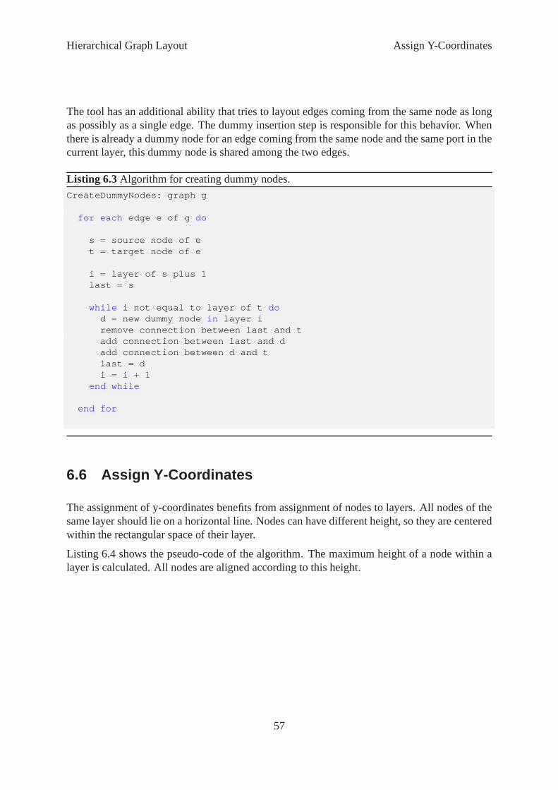
Hierarchical Graph Layout Assign Y-Coordinates
The tool has an additional ability that tries to layout edgescoming from the same node as longas possibly as a single edge. The dummy insertion step is responsible for this behavior. Whenthere is already a dummy node for an edge coming from the same node and the same port in thecurrent layer, this dummy node is shared among the two edges.
Listing 6.3 Algorithm for creating dummy nodes.CreateDummyNodes: graph g
for each edge e of g do
s = source node of et = target node of e
i = layer of s plus 1last = s
while i not equal to layer of t dod = new dummy node in layer iremove connection between last and tadd connection between last and dadd connection between d and tlast = di = i + 1
end while
end for
6.6 Assign Y-Coordinates
The assignment of y-coordinates benefits from assignment ofnodes to layers. All nodes of thesame layer should lie on a horizontal line. Nodes can have different height, so they are centeredwithin the rectangular space of their layer.
Listing 6.4 shows the pseudo-code of the algorithm. The maximum height of a node within alayer is calculated. All nodes are aligned according to thisheight.
57

Hierarchical Graph Layout Crossing Reduction
Listing 6.4 Algorithm for assigning y-coordinates.SetYCoordinate: graph gbase = 0for each layer l of g do
max = maximum height of a node in layer lfor each node n of layer l doy coordinate of n = base + (max - height of n)/2
end ifbase = base + max + vertical node offset
end for
Figure 6.4 shows the values calculated by the algorithm whenaligning a node. The node D ofthe example graph is centered. In its layer, the node E is the node with maximum height.
DEmax
base
height
(max – height)/2
Figure 6.4: Calculations when assigning y-coordinates.
This simple y-coordinate assignment step can be enhanced byallowing a variable vertical offsetbetween the layers. When the edges between two layers connect nodes that have a high hori-zontal offset, it is reasonable to increase the vertical offset to avoid sharp bends. In this case,the y-coordinate assignment step must be applied after the x-coordinate assignment.
6.7 Crossing Reduction
Until now the order of the nodes within their layer was arbitrary and did not affect any of theprocessing steps. The crossing reduction step tries to find an order that minimizes the edgecrossings of the graph.
Let n1 and m1 be two nodes in the first layer and n2 and m2 be two nodes in the second layer.Two edges (from n1 to n2 and from m1 to m2) cross if and only if the order between n1 andm1 in the first layer is opposite to the order between n2 and m2 in the second layer. To simplifythe analysis, the crossing reduction algorithms often optimize the crossings locally betweentwo layers. Finding an optimal solution that minimizes the crossings is NP-complete even forgraphs that have only two layers. Therefore, heuristics need to be applied that give good resultsin the normal case.
The algorithm iteratively sweeps down and up the layers. When sweeping down, the nodes oflayer i+1 are reordered by looking at the edges from layer i tolayer i+1. When sweeping up, the
58

Hierarchical Graph Layout Crossing Reduction
nodes of layer i are reordered by looking at the edges from layer i to layer i+1. Listing 6.5 showsthe pseudocode for a single downsweep. The new relative position of a node is calculated byforming the mean of the positions of its predecessor nodes. When sweeping up, the successornodes are used respectively. After calculating the relative position for all nodes in a layer, theyare reordered according to that position. The number of iterations is arbitrary, acceptable resultscan be achieved with only one or two iterations.
Listing 6.5 Crossing reduction algorithm.DownSweep: graph gfor the second to the last layer of g do
for each node n in layer i of g dosum = sum of the position of all predecessors of ncrossing number of n = sum / number of predecessors
end forresort the nodes in the list of layer i according to crossing number
end for
Figure 6.5 shows the downsweep step at layer 2 and 3 of the example graph. B and C arenumbered 1 and 2 according to their position within their layer. The only predecessor of E isC, so E gets a relative position of 2. D has two predecessors, so the mean of the position of itspredecessors is calculated and D gets a relative position of1.5. The dummy node has only onepredecessor, so it gets the relative position its only predecessor.
After reordering the nodes, the dummy node becomes the new first node, D stays in the middleand E becomes the new last node of layer three. When calculating the relative positions for thenodes in the next layer, the new positions 1, 2 and 3 are used.
B C
DE
1 2
2
B C
DE
1 2
2(1+2)/2 = 1.5
B C
DE
1 2
21.5
1
B C
D E
1 2
3 (2)2 (1.5)
1 (1)
Process E Process D Process dummy node Reorder
Figure 6.5: Crossing reduction applied on a layer of the example graph.
59

Hierarchical Graph Layout Assign X-Coordinates
6.8 Assign X-Coordinates
In this section, two different approaches for assigning x-coordinates to the nodes are presented.The inputs to these algorithms are a graph that fulfills the postconditions of the dummy insertionstep, the widths of the nodes, and the horizontal space requirements between nodes.
The goal of x-coordinate assignment is to find an x-coordinate for every node meeting the spacerequirements of the nodes. A subgoal is to minimize the totalhorizontal length of all edges.Another consideration is that the graph should look symmetric.
Both methods iteratively improve the layout of the graph, the number of iterations influencesthe layout quality. The order of the nodes within a layer is taken unchanged from the crossingreduction step.
6.8.1 DAG Method
After the initial layouting, the algorithm sweeps iteratively up and down the graph. In theremaining section only the downsweep is described. The upsweep works in a similar manner,but the outgoing instead of the incoming edges of a node are processed and the successors areused instead of the predecessors.
The initial positioning is arbitrary, however less iterations are needed if the first positioningis reasonable. One possibility is to align all nodes as left-most as possible meeting the spacerequirements of the nodes.
All nodes of a layer are repositioned in a special sequence: Nodes with less incoming edges areprocessed first. A node with a low degree in a bad position catches someone’s eye more thana node with a high degree in a bad position. Additionally, alledges between dummy nodes areprocessed first. This way long edges, which are split across several edges connecting dummynodes, are drawn as straight lines.
Then, the optimal position of a node is calculated as the median of the positions of its pre-decessors. This minimizes the horizontal length of the incoming edges. If the node has aneven number of predecessors, the mean of the two median predecessors is taken to increase thesymmetry of the drawing.
Listing 6.6 presents the pseudo-code for the downsweep partalgorithm. After the optimal x-coordinate was calculated, positioning a node works exactly the same way for both up- anddownsweep.
The final position of a node must take the layout constraints into account. If no other nodeon that layer is already positioned, we can just set the x-coordinate of the node to the optimalposition. Otherwise there is a range of legal positions thatmust be considered.
60

Hierarchical Graph Layout Assign X-Coordinates
Listing 6.6 Algorithm for assigning x-coordinates.DownSweep: graph gfor i from 2 to layer count of g do
l = all nodes in layer isort l in increasing order of predecessor countfor each node n in l dopos = median of predecessor positionsAddNode(n, pos)
end forend for
AddNode: node n, optimal position pleft = nearest already positioned node to the left of nright = nearest already positioned node to the right of nminX = position of left + width of left + horizontal node offsetmaxX = position of right minus width of rightincrease minX by width and offset of all nodes between left and ndecrease maxX by width and offset of all nodes between n and rightif pos < minX then
pos = minXelse if pos > maxX then
pos = maxXend ifposition of n = pos
In the code listing, the methodAddNode gives a pseudo-code representation of how the finalposition is calculated. Figure 6.6 shows graphically the allowed range for an example node X,that should be placed. Nodes L and R are the first nodes to the left and the right of X that arealready positioned.left_offset is the minimum space required for all nodes between Land X.right_offset is the minimum space required for all nodes between X and R plusthe width of X itself.
So the x-coordinate of X must be in the range betweenminX andmaxX. When the optimalposition lies outside this range, then the x-coordinate is either set tominX andmaxX, whicheveris closer to the optimal position.
Finding the nearest already positioned nodesleft andright can be done in O(log(n)) time,where n denotes the total number of nodes, using a balanced binary tree. The number of neces-sary iterations to get an acceptable result is low, a value oftwo is used by the tool. Therefore,the total time complexity of the algorithm is O(n*log(n)).
61

Hierarchical Graph Layout Assign X-Coordinates
L R
XL R
left right
minX maxX
left_offset right_offsetallowed range for X
Figure 6.6: X-coordinate assignment example.
6.8.2 Rubber Band Method
Another way to assign x-coordinates to the nodes uses a physical model and is called rubberband method. The algorithm presented in this section was developed by Georg Sander [25][26].The nodes of the graph are regarded as balls and the edges are rubber bands affecting the nodes.The vertical position of the nodes is fixed, so they can only move horizontally. Long edgesrepresented by dummy nodes would be skewed, so their x-coordinates are fixed to a singlevalue. They can be regarded as sticks.
Listing 6.7 presents the rubber band algorithm in pseudo-code. First, segments are formedout of nodes. A segment is regarded by the layout algorithm asa rectangular entity that canspan across several layers. Each segment will get a single x-coordinate assigned. Basically, asegment is represented by exactly one node. Only dummy nodesrepresenting the same edgeare merged into a single segment to assure that the edge is drawn as a straight line.
The algorithm constructs a graph with the segments as nodes and an edge between two segments(s and t) if and only if s contains a node that is the immediate left neighbor of a node of t.Based on this graph, a topological ordering of the segments is calculated. Afterwards, theyare positioned as left as possible. Segments without predecessors in the intermediate graphare positioned at the minimum x-coordinate. The leftmost possible x-coordinate for the othersegments is calculated by taking the maximum of the right boundary of all its predecessors. Thetopological sorting ensures that the predecessors of a segment are processed before the segmentitself is processed.
On this initial ordering, the physical model is now applied iteratively. The algorithm usuallyproduces a reasonable layout faster when in a downsweep onlythe predecessors of a node andin an upsweep only the successors of a node are taken into account. It is however also possibleto incorporate both predecessors and successors in the calculations, in the code listing this wayto calculate the forces is used.
Two segments that touch and whose forces cross are combined to a single region to conformbetter to the physical reality. So the algorithm starts by putting every segment into a single
62

Hierarchical Graph Layout Assign X-Coordinates
region. When two such interacting regions are found, they are removed from the set of regionsand the combined region is added.
The desired position for a region is its old position plus theforce on the region. The region ismoved to this position, however stopping when touching any other region. There is no specificprocessing order of the regions, and the result can vary according to this order. A high numberof iterations should however balance this.
Listing 6.7 Rubber-band algorithm for assigning x-coordinates.RubberBand: graph ggenerate segmentssort segments topologicallyset initial positionsfor i from 1 to MAX_ITERATIONS do
Process(g)end for
Process: graph gfor each segment s of g do
force on s = mean of predecessors and successors horizontal offsetsend for
regions of g = new set of regions with one region for each segmentfor each region r of g do
for each region t contacting r on the right doif force on r > force on t then
combine the regions of r and tend if
end forend for
for each region r of g doposition p = old position of r + force on rmove r to p stopping when hitting another region
end for
Figure 6.7 shows the main parts of the algorithm. In a preprocessing step, the nodes are groupedinto segments. In this example, the two dummy nodes are grouped into a single segment. Thethird graph shows the edges of the graph used for topologicalsorting and one legal topologicalsorting expressed by the numbers of the nodes. It also shows the initial positioning. The fourthgraph shows the regions created when performing a downsweep. The segments 2, 3, and 4 haveonly node 1 as their predecessor. If there were no other segments, the rubber band would movethem exactly under the segment 1. But in the example, the three segments would hit another andmove together such that they are all three side by side centered under node 1. So the algorithmcombines the three segments to a single region. Nodes 6 and 7 represent a similar case. Thefifth graph shows the segments with the x-coordinates assigned after the first downsweep.
63

Hierarchical Graph Layout Cluster Layout
When continuing with an upsweep, the regions must be recalculated. Now only the two seg-ments 3 and 4 are interacting. After a few iterations, the positions of the segments are translatedto positions of the nodes of the original graph.
4
5
6 7
3
2
1
4
5
6 7
3
2
1
4
5
6 7
3
2
1
4
5
6 7
3
2
1
4
5
6 7
3
2
1
Input Graph Segments Topological Sorting Regions at Downsweep
After Downsweep Regions at Upsweep After Upsweep Result
Figure 6.7: X-coordinate assignment using the rubber band method.
6.9 Cluster Layout
The general goal of clustering is to layout nodes of the same cluster close together. The visu-alization application draws a rectangle around nodes belonging to the same cluster. Therefore,the nodes need to be positioned in rectangular regions, suchthat the application can draw thecluster rectangles without intersections. This is achieved by first layouting each cluster sepa-rately and then performing the hierarchical layout recursively by treating the cluster rectanglesas nodes.
64

Hierarchical Graph Layout Drawing of Backedges
Figure 6.8 shows a simple clustered graph with two nodes. Node A is assigned to cluster 1, nodeB is assigned to cluster 2. There is a connection between A andB. First, the connection is splitinto three parts by inserting two intermediate nodes. The leftmost graph shows the resultingstructure. The connection between A and B is split into an edge going from A to a dummynode, an edge to another dummy node, and a third edge going to B. The dummy nodes havea dual function: When performing the separate layout of the clusters, they are treated just likedummy nodes. However, when performing the global layout, they are slots of the nodes thatrepresent the rectangular cluster areas.
First, the application performs the layout algorithm on thetwo blocks separately. The dummynode, which is a successor of node A, is always put in the last layer. The dummy node, which isa predecessor of node B, is put in the first layer. After the layout for the two blocks is calculated,the width and height of the rectangle encapsulating all nodes of a cluster is known. Then, anartificial graph is built: The cluster rectangles form the nodes and the two dummy nodes formslots. The hierarchical layout algorithm is applied again on the artificial cluster graph.
C1
C2
A
Output Slot
Input Slot
Edge
Last Layer Dummy Node
B
First Layer Dummy Node
Layout Cluster 2
Layout Cluster 1 Global Layout
C1
C2
Clustered Input Graph
A
B
Figure 6.8: Recursive cluster layout.
6.10 Drawing of Backedges
In Section 6.3, an algorithm for reversing edges to make the input graph free of cycles waspresented. The visualization tool always paints edges suchthat they start at the bottom of anode and end at a top of a node. For backedges, a special routing for adding interpolation pointis needed.
All backedges are processed in a right-to-left order. The additional interpolation points and theport are calculated as shown in Figure 6.9. A node with backedges will not only get new ports,but also change its size. The horizontal and vertical space needed for the backedges are addedto the size of the node.
65

Hierarchical Graph Layout Optimization for Large Graphs
Additional Ports
Interpolation Points
Figure 6.9: Example for the routing of a backedge.
6.11 Optimization for Large Graphs
When the server compiler processes long Java methods, the resulting graph is so large thatthe time for performing the layout is annoying for the user. The graph of the server compilercontains a high number of edges, which leads to some edges nearly spanning over the wholegraph. Long edges are a problem for two reasons: First, a lot of dummy nodes need to becreated and later processed by the coordinate assignment and the crossing reduction. Second,they disturb the drawing, because they are represented by long straight lines and the nodes alongtheir way are either drawn on the right or on the left.
The benefit of drawing the long edges is not high, because mostly only a small part of them isvisible. An edge that starts and ends outside of the current screen extract is not informative.Therefore, the visualization application cuts long edges and draws only their beginning andending. This way, the drawing performance as well as the quality of the drawing is improved.
66

Chapter 7
Compiler Instrumentation
This chapter describes the coded added to the Java HotSpotTM server compiler. The currentversion is based on JDK 7 build 13 [16]. The design goal for theinstrumentation was to changeas little code of the server compiler as possible and to encapsulate the added code.
7.1 Overview
Figure 7.1 shows the classes added to the server compiler andhow they are connected to alreadyexisting classes.IdealGraphPrinter is the main class that manages the tracing of thegraphs. As explained in Section 5.2.1, a graph is serializedas the difference to the previousgraph. The server compiler does not store old versions of thegraph, so the graph printer objectmust handle this.Description objects are used for this purpose.
When printing a graph, first theDescription objects of the previous graph are marked asinvalid. Description objects of the new graph start with the statenew. If the new objectequals an old one, then the new one replaces the old one and gets the statevalid. For aninvalid Description object, only a mark that it has been removed is stored. A validDes-cription object needs no storage space at all, as it was serialized with the previous graph.Only for newDescription objects, the graph printer outputs the full data.
Description has two subclasses:EdgeDescription andNodeDescription. Anobject of classEdgeDescription has a reference to the start and end node of the edge. Itstores the input index at which the edge enters the end node. The server compiler works withan object of classCompile, which consists ofNode objects. ANodeDescription objectstores a reference to the describedNode object. It is an object that has properties represented bystring key-value pairs. The C++ memory address of aNode object forms the unique identifierof a node.
The scheduler constructs a control flow graph by grouping thenodes into blocks (see Sec-tion 7.2). This process is repeated for every graph. The control flow graph is not stored
67

Compiler Instrumentation Identifying Blocks
difference-based like the normal graph, because a small change in the normal graph can causea big change in the control flow graph.
EveryCompileThread object has its ownIdealGraphPrinter object to avoid multi-threading conflicts. The graph printer uses thePhaseChaitin class to get information aboutthe selected registers and life ranges of the nodes (for details on the register allocation see Sec-tion 3.6). TheMatcher class is used to retrieve the matcher flags that identify the subtrees ofthe graph, which are converted toMachNode objects (see Section 3.5).
For actually outputting the data, the printer either uses the fileStream class of the servercompiler or thenetworkStream class. They are both subclasses ofoutputStream.
networkStream IdealGraphPrinter
Property
Properties
state: invalid, valid or new
Description
NodeDescription
Block
EdgeDescription
*
outputStream
CompilerThreadfileStream
Compile
Node
Server Compiler
*
PhaseChaitin
Matcher
0..1
0..1 *
Ideal Graph Printer
is assigned to
Figure 7.1: Compiler instrumentation class diagram.
7.2 Identifying Blocks
The nodes of the ideal graph are ungrouped. The control flow isonly expressed as controldependence edges. The printer schedules the nodes into blocks to allow the visualization appli-cation to group the nodes. This increases the overview of thegraph and is essential for largemethods.
68

Compiler Instrumentation Identifying Blocks
In a first step, all nodes that are related to control flow, i.e.either have a control dependenceinput or output edge, are assigned to blocks. The control dependencies link the control flowrelated nodes of a block together in a linear list. This ensures that there are no branches in ablock. The start node is either a node that joins several control flow dependencies, e.g. aRe-gion node, or a node that represents a successor of a node that splits control flow, e.g. anIfnode. The end node of a block is either a node that is the predecessor of a node that joins controlflow or a node that splits control flow.
The algorithm processes the graph in reversed order, starting at theRoot node. Figure 7.2shows the steps applied for each node that is popped from the stack. When the node was notvisited before, it forms the end of a new basic block. The algorithm walks up the graph alongthe control dependence edges and adds the nodes to the same block. The end of the walk isreached when the algorithm either finds a node marked as blockprojection, i.e. a successornode of a node that splits control flow, or a node marked asblock_start, e.g. aRegionnode. This last node is the start node of the block and its predecessors are pushed onto the stack.Listing 7.1 presents the pseudo-code for identifying basicblocks.
Listing 7.1 Algorithm for identifying blocksFindBlocks: graph gpush root node of g onto stack
while stack not empty donode n = pop from stackif n not visited then
mark n as visitedcreate new block badd n to b
while n not block_proj and n not block_start don = control dependence predecessor of padd n to b
end while
for each node p in predecessors of n dopush p onto stack
end forend if
end for
69

Compiler Instrumentation Building Dominator Tree
... ...
Node popped from stack
End node of block
Intermediate nodes
Start node of block
Block Projection Region Node
New nodes pushed onto stack
Figure 7.2: Steps applied for identifying a block.
7.3 Building Dominator Tree
A block is the dominator of another block if it is always executed before the other block isexecuted. Knowing the dominators is essential for scheduling the nodes, because the argumentsof an operation must be executed in all control paths. Therefore, the operands of an operationmust be either in the same block or in one of the dominators of the block of the operation itself.A block a is the immediate dominatorof another blockb, if all other dominators of blockbdominate blocka. The dominator tree consists of the blocks as nodes and edgesbetween ablock and its immediate dominator. The immediate dominatorof a block is the parent of theblock in the dominator tree. The start block of a method dominates all other blocks. Therefore,it is the root of the dominator tree.
There is an iterative O(n2) solution for calculating the dominators of all nodes of a graph.It starts by initializing the set of dominators of each node to the full set of all nodes. Thenthe algorithm reduces the dominator set of the root node to only the root node itself. Thealgorithm uses the following rule to iteratively update thedominator sets of the other nodes: Thedominator set of a node is the conjunction of the dominator sets of its predecessors. If a nodedominates all predecessors of another node, it must also dominate that node too. Additionally,
70

Compiler Instrumentation Building Dominator Tree
the node itself is always kept in its the dominator set. The algorithm iteratively updates thedominator sets until a full iteration over all nodes brings no further changes.
Lengauer and Tarjan [19] present a faster algorithm for calculating the immediate dominators,which runs in O(n*log(n)) time. First, the algorithm numbers the nodes of the graph based ona depth-first search traversal and stores the parents of a node in the depth-first search tree. Thedepth first tree has some special properties that are useful when calculating the dominators. Aparent node in the depth-first tree has a lower number than allits children. As the dominator ofa node is always reached on any path from the root to the node, it must also be reached by thedepth-first search algorithm before the node itself is reached. There cannot be another way toreach the node. Therefore, the dominator of a node is an ancestor of the node in the depth-firstsearch tree.
The second step of the algorithm is to calculatesemi-dominators, i.e. approximate dominatorsthat are later used to calculate the immediate dominators. Dominator candidates for a node areall nodes that are ancestors of the node in the depth-first search tree. Another node cannot be thedominator of that node, because there would be another path from the root to that node usingthe ancestors of the depth-first tree. When a node has only onepredecessor, this predecessormust be the dominator of that node. There cannot be a path thatreaches that node without usingthe edge from its predecessor to the node.
When there are two possible paths from node a to node b, then the depth-first search numbers ofthe second path are all higher than the numbers of node b. The semi-dominator of a node is thenode closest to the root that is the start of two possible paths to that node. Figure 7.3 shows therelations between a node, its semi-dominator and the root node. The nodes between the nodeand its semi-dominator in the depth-first search tree cannotbe dominators of the node, becausethere exists an alternative path from the root to the node.
...
Node
Semi-Dominator
...Path in DFS treeAny path, all nodes with
higher DFS numbers
Root Node
...
Figure 7.3: Calculation of the semi-dominators.
The semi-dominator is not necessarily the real immediate dominator of a node, because theremight exist a path from the root node to one of the nodes between the node and the semi-dominator, which does not contain the semi-dominator. The dominator is always the semi-dominator, the root, or it lies between the semi-dominator and the root in the depth-first searchtree.
71

Compiler Instrumentation Building Dominator Tree
Node
Semi-Dominator
Root Node
...
Node with minimum
semi-dominator
...
...
Case 1: Minimum semi-dominator = semi-dominator
Case 2: Minimum semi-dominator < semi-dominator
Figure 7.4: Calculation of the dominators.
Figure 7.4 shows the two cases that arise when calculating the immediate dominator of a node.First, the algorithm runs through the nodes between the nodeand its semi-dominator in thedepth-first search tree. It selects the node that has the semi-dominator with the minimum depth-first search number. If this minimum semi-dominator is equalto the node’s semi-dominator,then the node’s dominator is equal to the node’s semi-dominator. Otherwise, the node’s domi-nator is equal to the dominator of the node with the minimum semi-dominator.
1
6 2
3
4
1 / 1
5 / 1 2 / 1
3 / 1
4 / 25 5 / 3
1 / 1 / 1
5 / 1 / 1 2 / 1 / 1
3 / 1 / 1
4 / 2 / 15 / 3 / 3
Initial Graph Assigning DFS Number Semi-Dominators Dominators
Figure 7.5: Algorithm for finding dominators applied on an example graph.
Figure 7.5 gives an example of a dominator calculation. First, the nodes are traversed in depth-first order and get a number assigned. The thick lines represent edges that are also present inthe depth-first search tree. Next, the semi-dominators are calculated. For example, the semi-dominator of node 3 is the node 1 as there exists a path (1 - 5 - 3)that visits only nodes with ahigher depth-first search number. The last step is the calculation of the immediate dominatorsbased on the semi-dominators. Node 4 represents a case in which the semi-dominator and thedominator differs. This is because the node 3 is between the node 4 and its semi-dominator, andthe semi-dominator of node 3 is the node 1, which has a lower number than the semi-dominator
72

Compiler Instrumentation Scheduling
of node 4. There exists an alternative path from the root to node 3 (1 - 5 - 3) that does not usethe semi-dominator node 2. Therefore, the dominator of node4 is equal to the dominator ofnode 3, which is the root node 1.
7.4 Scheduling
When scheduling nodes, the dominator tree plays a main role.A node has several input nodesthat form parameters and the result of a node is used by other nodes. Before a node itself isscheduled, all input nodes need to be evaluated. On the otherhand, a node must be scheduledbefore its result is used for the first time. Therefore, it must be scheduled in a block thatdominates all the blocks in which the node is used.
The graph printer uses a scheduling strategy that puts a nodein the latest possible block, i.e. inthe block that dominates all blocks in which the result of thenode is used. First, the dominatortree is constructed from the dominator information calculated by the algorithm of Lengauer andTarjan (see Section 7.3).
Figure 7.6 explains how the common dominator of two blocks iscalculated. First, the dominatortree is constructed. In this tree, each block is the child of its immediate dominator. Finding thecommon dominator of two blocks corresponds to finding the first ancestor of two blocks in thedominator tree. For example, the common dominator of F and E is the block B. The algorithmgoes from the block F upwards to the root and marks each visited block with a flag. Then, itgoes from the block E up to the root and the first block which hasthe flag set is the commondominator of the two blocks.
A
B G
C
ED
Initial Graph
H
Dominator Tree
A
B G
CD H
E
F
F
Common Dominator of E and F
A
B G
CD H
E
F
Figure 7.6: Finding common dominators.
The control flow related nodes are already scheduled (see Section 7.2). Now, the other nodesare scheduled iteratively: Whenever all successors of a node have been assigned to certainblocks, the node is put into the common dominator of the blocks of its successors. The commondominator of n blocks is equal to the common dominator of the last block and the commondominator of the first n-1 blocks.
73

Compiler Instrumentation Adding States
7.5 Adding States
Additional states of the graph can be traced by calling theprintmethod of the printer object ofthe current thread. A call to the static methodIdealGraphPrinter::printer() returnsthe current printer object orNULL if printing is disabled. Figure 7.7 explains the sequence,in which calls to the public methods of a graph printer objectare valid. The compiler threadsautomatically call the constructor and destructor of theirprinter objects at startup and shutdownof the VM. For every method, thenew_method function must be called before any graphs areprinted, and theend_method function must be called afterwards. In between, any number ofcalls to theprint method are allowed.
Start
constructornew_method
End
desctructorend_methodprint
Compile &c char *name
int level
Figure 7.7: Life cycle of anIdealGraphPrinter object.
When calling theprint method, the name and the level of the state must be specified. Thecall toprint is ignored when the level set by the user is lower than the level of the state.
Listing 7.2 lists the code necessary to add a new state. TheIdealGraphPrinter objectis obtained by a call to a static function. This function automatically returns the graph printerobject of the current compiler thread. It returnsNULL when printing graphs is disabled. In thisexample, the level of the new state is set to 2.
Listing 7.2 Code for adding a state.IdealGraphPrinter *printer = IdealGraphPrinter::printer();if (printer != NULL) {printer->print("New State", 2);
}
74

Chapter 8
Conclusions
In this thesis, a tool for the visualization of the graph datastructure of the Java HotSpotTM
server compiler was presented. It assists at debugging the server compiler and at understandingoptimization steps. The tool allows the analysis of large graphs and has built-in navigation andfiltering possibilities. It clusters the nodes of the graph based on control flow and displays thegraph using a hierarchical layout algorithm. Code in the server compiler allows the user togenerate data for the visualization tool by using a compilerflag.
One of the most challenging problems during the developmentof the tool was to understandthe graph of the server compiler. Its mixture of a control flowand a data dependence graph isless intuitive than the graph of the client compiler, which clearly separates these two concepts.The high number of edges of the graph in comparison to the nodecount is prejudicial to a cleardrawing. Difficult to handle are nodes that resemble shared variables such as the node for theframe pointer and the return address. They are defined in one place, but used very often in thegraph. The visualization tool uses a splitting filter for such nodes.
The first attempts to draw the graph ended up in a confusing scribble, even for small methods.A lot of time was necessary for incrementally increasing thedrawing by filters and better layoutalgorithms. Each of the optimizations contributes a littleto the clarity of the graph. Applyingall of them finally gives an acceptable drawing. The performance was also a big issue, becausethe graph of a large Java method can have a high number of nodesand edges. For such a graph,not only efficient layout algorithms are necessary, but alsoa user interface that allows to focuson specific parts of the graph.
One of the planned improvements is the enhancement of the drawing performance of the userinterface. Drawing performance is a critical issue, because the graph can contain a few thousandnodes with multiple slots and more than ten thousand edges with multiple interpolation points.
The Java HotSpotTM compiler group of Sun Microsystems is currently testing thetool on real-world examples. Based on these testing experiences, the tool will be further enhanced. Con-cerning the hierarchical layout algorithm, there are plansto integrate it into the official versionof the NetBeans visual library.
75

List of Figures
1.1 Conventions used in the class diagrams. . . . . . . . . . . . . . .. . . . . . . 22.1 Screenshot of Xelfi, the ancestor of NetBeans, running with JDK 1.1. . . . . . 62.2 Using lookup, there is no dependency between service user and service provider. 82.3 Class diagram of the NetBeans visual library. . . . . . . . . .. . . . . . . . . 102.4 Screenshot of the visual library example program duringexecution. . . . . . . 103.1 Architecture of the Java HotSpotTM Virtual Machine. . . . . . . . . . . . . . . 133.2 States during the execution of an example method. . . . . . .. . . . . . . . . 143.3 Architecture of the Java HotSpotTM server compiler of Sun Microsystems. . . . 163.4 Program dependence graph when processingp*100+1. . . . . . . . . . . . . 173.5 Graph when processing an empty method. . . . . . . . . . . . . . . .. . . . . 183.6 Graph when processing anif statement. . . . . . . . . . . . . . . . . . . . . . 193.7 SafePoint node after parsing 5+x+7. . . . . . . . . . . . . . . . . . . . . . 203.8 Identity optimization:(x+0) is transformed tox. . . . . . . . . . . . . . . . . 213.9 Constant folding:(5+p+7) is transformed to(p+12). . . . . . . . . . . . . 223.10 Global value numbering:(x+1)*(x+1) is transformed to(x+1)2. . . . . . 233.11 Nodes that define a counted loop. . . . . . . . . . . . . . . . . . . . .. . . . . 243.12 Matching and register allocation example. . . . . . . . . . .. . . . . . . . . . 254.1 Architectural overview. . . . . . . . . . . . . . . . . . . . . . . . . . .. . . . 284.2 Viewing a graph using the Java application. . . . . . . . . . . .. . . . . . . . 304.3 The satellite view gives an overview of a graph. . . . . . . . .. . . . . . . . . 324.4 Four functions applied to an example graph. . . . . . . . . . . .. . . . . . . . 354.5 Bytecode Window showing the Java bytecodes in tree-form. . . . . . . . . . . 365.1 Dependencies of the NetBeans modules. . . . . . . . . . . . . . . .. . . . . . 385.2 Lifecycle of the graph data. . . . . . . . . . . . . . . . . . . . . . . . .. . . . 405.3 XML file structure. . . . . . . . . . . . . . . . . . . . . . . . . . . . . . . . .415.4 Data module class diagram. . . . . . . . . . . . . . . . . . . . . . . . . .. . . 425.5 Display model class diagram. . . . . . . . . . . . . . . . . . . . . . . .. . . . 435.6 Layout model class diagram. . . . . . . . . . . . . . . . . . . . . . . . .. . . 445.7 Properties and selectors class diagram. . . . . . . . . . . . . .. . . . . . . . . 465.8 Filters class diagram. . . . . . . . . . . . . . . . . . . . . . . . . . . . .. . . 475.9 The difference algorithm applied on two example graphs.. . . . . . . . . . . . 496.1 Steps of a hierarchical layout algorithm. . . . . . . . . . . . .. . . . . . . . . 526.2 Breaking cycles of an example graph. . . . . . . . . . . . . . . . . .. . . . . 54
76

6.3 Assigning layers for the nodes of the example graph. . . . .. . . . . . . . . . 566.4 Calculations when assigning y-coordinates. . . . . . . . . .. . . . . . . . . . 586.5 Crossing reduction applied on a layer of the example graph. . . . . . . . . . . . 596.6 X-coordinate assignment example. . . . . . . . . . . . . . . . . . .. . . . . . 626.7 X-coordinate assignment using the rubber band method. .. . . . . . . . . . . 646.8 Recursive cluster layout. . . . . . . . . . . . . . . . . . . . . . . . . .. . . . 656.9 Example for the routing of a backedge. . . . . . . . . . . . . . . . .. . . . . . 667.1 Compiler instrumentation class diagram. . . . . . . . . . . . .. . . . . . . . . 687.2 Steps applied for identifying a block. . . . . . . . . . . . . . . .. . . . . . . . 707.3 Calculation of the semi-dominators. . . . . . . . . . . . . . . . .. . . . . . . 717.4 Calculation of the dominators. . . . . . . . . . . . . . . . . . . . . .. . . . . 727.5 Algorithm for finding dominators applied on an example graph. . . . . . . . . 727.6 Finding common dominators. . . . . . . . . . . . . . . . . . . . . . . . .. . . 737.7 Life cycle of anIdealGraphPrinter object. . . . . . . . . . . . . . . . . 74
77
Code Listings
2.1 An XML layer file defining an action and hiding a menu item. .. . . . . . . . 72.2 Java source code of a visual library program with a label widget and an action. . 113.1 Architecture description file extract. . . . . . . . . . . . . . .. . . . . . . . . 265.1 Algorithm for calculating the difference between two graphs. . . . . . . . . . . 496.1 Algorithm for breaking cycles in a directed acyclic graph. . . . . . . . . . . . . 536.2 Algorithm for assigning layers. . . . . . . . . . . . . . . . . . . . .. . . . . . 556.3 Algorithm for creating dummy nodes. . . . . . . . . . . . . . . . . .. . . . . 576.4 Algorithm for assigning y-coordinates. . . . . . . . . . . . . .. . . . . . . . . 586.5 Crossing reduction algorithm. . . . . . . . . . . . . . . . . . . . . .. . . . . 596.6 Algorithm for assigning x-coordinates. . . . . . . . . . . . . .. . . . . . . . . 616.7 Rubber-band algorithm for assigning x-coordinates. . .. . . . . . . . . . . . . 637.1 Algorithm for identifying blocks . . . . . . . . . . . . . . . . . . .. . . . . . 697.2 Code for adding a state. . . . . . . . . . . . . . . . . . . . . . . . . . . . .. . 74
78

Bibliography
[1] A Brief History of NetBeans, URL: http://www.netbeans.org/about/history.html, 2007.
[2] Tim Boudreau, Jaroslav Tulach, and Geertjan Wielenga,Rich Client Programming: Plug-ging into the NetBeans Platform, Prentice Hall, 2007.
[3] Preston Briggs, Keith D. Cooper, and Linda Torczon,Improvements to Graph Color-ing Register Allocation, In ACM Transactions on Programming Languages and Systems,ACM Press, 16, 428-455, 1994.
[4] Preston Briggs, Keith D. Cooper, and L. Taylor Simpson,Value Numbering, Software:Practice and Experience 27, 6, 701-724, 1997.
[5] Gregory Chaitin,Register Allocation and Spilling via Graph Coloring, In Proceedings ofthe 1982 SIGPLAN Symposium on Compiler Construction, ACM Press, 98-105, 1982.
[6] Cliff Click, Global Code Motion/Global Value Numbering, In Proceedings of the ACMSIGPLAN 1995 Conference on Programming Language Design andImplementation,ACM Press, 246-257, 1995.
[7] Cliff Click and Keith D. Cooper,Combining Analyses, Combining Optimizations, In ACMTransactions on Programming Languages and Systems, ACM Press, 17, 181-196, 1995.
[8] Cliff Click and Michael Paleczny,A Simple Graph-Based Intermediate Representation, InACM SIGPLAN Workshop on Intermediate Representations, ACMPress , 1995.
[9] Ron Cytron, Jeanne Ferrante, Barry K. Rosen, Mark N. Wegman, and F. Kenneth Zadeck,Efficiently Computing Static Single Assignment Form and theControl Dependence Graph,In ACM Transactions on Programming Languages and Systems, ACM Press, 451-490,1991.
[10] Jeanne Ferrante, Karl J. Ottenstein, and Joe D. Warren,The Program Dependence Graphand its Use in Optimization, In ACM Transactions on Programming Languages and Sys-tems, ACM Press, 9, 319-349, 1987.
[11] Emden R. Gansner, Stephen C. North, and Kiem-Phong Vo,DAG - A Program that DrawsDirected Graphs, In Software, Practice and Experience 18, John Wiley & Sons,11, 1047-1062, 1988.
79

[12] Emden R. Gansner, Eleftherios Koutsofios, Stephen C. North, and Kiem-Phong Vo,ATechnique for Drawing Directed Graphs, In IEEE Transactions on Software Engineering19, 214-230, 1993.
[13] Graph Visualization Software (GraphViz), URL: http://www.graphviz.org, 2007.
[14] Graph Layout Software aiSee, URL: http://www.aisee.com, 2007.
[15] Robert Griesemer and Srdjan Mitrovic,A Compiler for the Java HotSpot Virtual Machine,In The School of Niklaus Wirth, "The Art of Simplicity", dpunkt.verlag, 133-152, 2000.
[16] Java Platform Standard Edition 7 Source, URL: http://jdk7.dev.java.net, 2007.
[17] Java HotSpot Client Compiler Visualizer, https://c1visualizer.dev.java.net, 2007.
[18] Thomas Kotzmann, Christian Wimmer, Hanspeter Mössenböck, Thomas Rodriguez, Ken-neth Russell, and David Cox,Design of the Java HotSpot Client Compiler for Java 6,Technical Report, 2007.
[19] Thomas Lengauer and Robert E. Tarjan,A Fast Algorithm for Finding Dominators in aFlowgraph, In ACM Transactions on Programming Languages and Systems,ACM Press,121-141, 1979.
[20] Stefan Loidl,Compiler Data Flow Visualization, Master’s Thesis at the Johannes KeplerUniversity Linz, 2007.
[21] Adam Myatt,Pro NetBeans IDE 5.5 Enterprise Edition, Apress, 2007.
[22] NetBeans, URL: http://www.netbeans.org, 2007.
[23] Michael Paleczny, Christopher Vick, and Cliff Click,The Java HotSpot Server Compiler,In Proceedings of the Java Virtual Machine Research and Technology Symposium, 1-12,USENIX, 2001.
[24] Eduardo Pelegrí-Llopart and Susan L. Graham,Optimal Code Generation for ExpressionTrees: an Application BURS Theory, In Proceedings of the 15th ACM Symposium onPrinciples of Programming Languages, ACM Press, 294-308, 1988.
[25] Georg Sander,Graph Layout Through the VCG Tool, In Proceedings of the DIMACSInternational Workshop on Graph Drawing, Springer-Verlag, 194-205, 1994.
[26] Georg Sander,A Fast Heuristic for Hierarchical Manhattan Layout, In Proceedings of theSymposium on Graph Drawing, Springer, 447-458, 1996.
[27] Georg Sander,Visualization of Compiler Graphs (VCG), URL: http://rw4.cs.uni-sb.de/~sander/html/ gsvcg1.html, 2007.
[28] Bill Joy, Guy Steele, James Gosling, and Gilad Bracha,The Java(TM) Language Specifi-cation (Third Edition), Prentice Hall, 2005.
80

[29] Tim Lindholm and Frank Yellin,The Java(TM) Virtual Machine Specification (SecondEdition), Prentice Hall, 2007.
[30] uDraw(Graph), URL: http://www.informatik.uni-bremen.de/uDrawGraph, 2007.
[31] Christian Wimmer and Hanspeter Mössenböck,Optimized Interval Splitting in a LinearScan Register Allocator, In Proceedings of the ACM/USENIX International Conferenceon Virtual Execution Environments, ACM Press, 132-141, 2005.
[32] Thomas Würthinger,Visualization of Java Control Flow Graphs, Bachelor’s Thesis at theJohannes Kepler University Linz, 2006.
[33] Xelfi, URL: http://tecfa.unige.ch/pub/software/win95/langages/java/xelfi, 2007.
81