Embed Size (px)
Citation preview

VISUALIZATION OF CURVE AND SURFACE
DATA USING RATIONAL CUBIC BALL
FUNCTIONS
WAN NURHADANI BINTI WAN JAAFAR
UNIVERSITI SAINS MALAYSIA
2018

VISUALIZATION OF CURVE AND SURFACE
DATA USING RATIONAL CUBIC BALL
FUNCTIONS
by
WAN NURHADANI BINTI WAN JAAFAR
Thesis submitted in fulfillment of the requirements
for the degree of
Doctor of Philosophy
February 2018

ii
ACKNOWLEDGEMENT
In the name of Allah S.W.T, the Most Gracious and the Most Merciful. First and
foremost, I am most grateful to Allah, the One who gives me the strengths and the
knowledge to complete this unforgettable journey. For this opportunity, I would like
to thank those who helped me and encouraged me to complete this PhD journey.
Firstly, I would like to express my deepest gratitude and appreciation to my main
supervisor, Professor Dr. Abd. Rahni Mt Piah for his valuable guidance and advice
throughout this study. Secondly, I would like to thank my field supervisor, Dr.
Muhammad Abbas from University of Sargodha, Pakistan, who has constantly and
consistently help me. Most importantly, I would like to thank University Malaysia
Perlis and Ministry of Higher Education for the financial support during my PhD.
Last but not least, special thanks to my beloved parents Che Jamilah Sulong, Wan
Jaafar Wan Mohamad and all my friends, especially, Siti Jasmida, Hartini, Noor
Wahida, Ezzah Liana, Shakila and Nur Fatihah. Not to forget, all my lab friends and
the staffs at School of Mathematical Sciences, Universiti Sains Malaysia for their
undivided attention, motivation, support and advice.
iii
TABLE OF CONTENTS
ACKNOWLEDGEMENT .......................................................................................... ii
TABLE OF CONTENTS ........................................................................................... iii
LIST OF TABLES .................................................................................................... vii
LIST OF FIGURES ................................................................................................. viii
LIST OF ABBREVIATIONS ..................................................................................... x
LIST OF SYMBOLS ................................................................................................. xi
ABSTRAK…… ........................................................................................................ xii
ABSTRACT………………………………………………………………………..xiii
CHAPTER 1 - BACKGROUND OF STUDY AND LITERATURE REVIEW
1.1 Data Visualization .................................................................................................. 1
1.2 Shape Characteristics of Data and Applications .................................................... 3
1.2.1 Shape Characteristics ................................................................................... 3
1.2.2 Applications ................................................................................................. 7
1.3 Ball Functions and Advantages .............................................................................. 8
1.4 Continuity Conditions .......................................................................................... 14
1.5 Literature Review ................................................................................................. 15
1.5.1 Positivity Preserving Curve and Surface ................................................... 16
1.5.2 Monotonicity Preserving Curve and Surface ............................................. 21
1.5.3 Convexity Preserving Curve and Surface .................................................. 25
1.5.4 Constrained Preserving Curve and Surface ............................................... 28
1.6 Motivation of Study ............................................................................................. 29
1.7 Objectives of Study .............................................................................................. 31
1.8 Outline of the Thesis ............................................................................................ 32

iv
CHAPTER 2 - RATIONAL CUBIC BALL WITH SHAPE CONTROL
2.1 Introduction .......................................................................................................... 35
2.2 1C Rational Cubic Ball Interpolant ..................................................................... 36
2.3 Shape Control Analysis ........................................................................................ 37
2.4 Conclusion ........................................................................................................... 49
CHAPTER 3 - SHAPE PRESERVING RATIONAL CUBIC BALL CURVE
INTERPOLATION WITH FOUR SHAPE PARAMETERS
3.1 Introduction .......................................................................................................... 51
3.2 Rational Cubic Ball Function with Four Shape Parameters................................. 53
3.2.1 Shape Preserving C1 Curve Visualization.................................................. 54
3.3 Positivity Preserving Rational Cubic Ball Interpolation ...................................... 55
3.4 Monotonicity Preserving Rational Cubic Ball Interpolation ............................... 59
3.5 Constrained Rational Cubic Ball Interpolation .................................................... 63
3.6 Shape Preserving Rational Cubic Bézier to Rational Cubic Ball using ............... 67
Conversion ........................................................................................................... 67
3.6.1 Definition Rational Cubic Bézier Function and Rational Cubic Ball ........ 68
Function ..................................................................................................... 68
3.7 Conversion Matrices between Rational Cubic Bézier Curve and Rational ......... 70
Cubic Ball Curve .................................................................................................. 70
3.7.1 Coefficients Matrix of Bézier Curve.......................................................... 70
3.7.2 Coefficients Matrix of Ball Curve ............................................................. 71
3.8 Relationship of Weights and Control Points between Rational Cubic Bézier ..... 72
Curve and Rational Cubic Ball Curve .................................................................. 72

v
3.9 Rational Cubic Ball Interpolation using Conversion Control Points and ............ 74
Weights ................................................................................................................ 74
3.10 Positivity Rational Cubic Ball with Conversion Interpolation .......................... 75
3.11 Monotonicity Rational Cubic Ball with Conversion Interpolation .................... 78
3.12 Convexity Rational Cubic Ball with Conversion Interpolation ......................... 82
3.13 Constrained Rational Cubic Ball with Conversion Interpolation ...................... 87
3.14 Conclusion ......................................................................................................... 90
CHAPTER 4 - SHAPE PRESERVING RATIONAL CUBIC BALL CURVE
INTERPOLATION WITH THREE SHAPE PARAMETERS
4.1 Introduction ......................................................................................................... 93
4.2 Rational Cubic Ball Function with Three Shape Parameters ............................... 94
4.3 Shape Preserving C1 Curve Visualization ............................................................ 95
4.4 Positivity Rational Cubic Ball Interpolation ........................................................ 96
4.5 Monotonicity Rational Cubic Ball Interpolation.................................................. 99
4.6 Convexity Rational Cubic Ball Interpolation ..................................................... 102
4.7 Constrained Rational Cubic Ball Interpolation .................................................. 105
4.9 Conclusion ......................................................................................................... 108
CHAPTER 5 - RATIONAL BI-CUBIC BALL SURFACE INTERPOLATION
5.1 Introduction ........................................................................................................ 110
5.2 Partially Blended Rational Bi-Cubic Ball Function (Coons Patches) ................ 111
5.3 Visualization of Positive Shaped Data by Partially Blended Rational .............. 115
Bi-Cubic Ball ..................................................................................................... 115

vi
5.4 Visualization of Monotonic Shaped Data by Partially Blended Rational .......... 121
Bi-Cubic Ball ..................................................................................................... 121
5.5 Visualization of Constrained Data by Partially Blended Rational Bi-Cubic ..... 129
Ball ..................................................................................................................... 129
5.6 Rational Bi-Cubic Ball Function (Tensor Product Patches) .............................. 138
5.7 Visualization of Positive Shaped Data by Rational Bi-Cubic Ball .................... 142
5.8 Visualization of Monotonic Shaped Data by Rational Bi-Cubic Ball ............... 147
5.9 Visualization of Constrained Data by Rational Bi-Cubic Ball .......................... 162
5.10 Conclusion ....................................................................................................... 174
CHAPTER 6 - CONCLUSION AND FURTHER WORKS
6.1 Conclusion ......................................................................................................... 178
6.2 Suggestion for Further Work ............................................................................. 181
REFERENCES……………………………………………………………………182
APPENDIX
LIST OF PUBLICATIONS

vii
LIST OF TABLES
Page
Table 2.1 Positive data set of molar volume of the gas [145]. 39
Table 2.2 A positive random data set A.1. 41
Table 3.1 A positive random data set A.2. 58
Table 3.2 2D monotone data set [13]. 62
Table 3.3 2D constrained data set [127]. 66
Table 3.4 2D positive random data set A.3. 78
Table 3.5 2D monotone data set [154]. 81
Table 3.6 2D convex of data set [155]. 86
Table 4.1: A positive set of chemical experiment data [73]. 98
Table 4.2 A random monotone set of cricket match data A.4. 102
Table 4.3 A 2D convex data set [161]. 104
Table 4.4 A constrained data set [130]. 108
Table 5.1 A positive surface data set [64]. 119
Table 5.2 A monotone random surface data set [168]. 127
Table 5.3 A random constrained surface data set [68]. 136
Table 5.4 A positive random surface data set [170]. 145
Table 5.5 A 3D monotone surface data set [171]. 160
Table 5.6 A 3D constrained surface data set [170]. 173
Table 5.7 Data set from plane [170]. 173
( , )W x y

viii
LIST OF FIGURES
Page
Figure 1.1 The flowchart of study. 34
Figure 2.1 The rational cubic Ball function with 2i i , 0.0001iu
and 1iv using (2.4). 39
Figure 2.2 The rational cubic Ball function with 2i i , 1iu and
0.0001iv using (2.5). 40
Figure 2.3 The rational cubic Ball function with 2i i and
0.3i iu v using (2.6). 40
Figure 2.4 Interpolatory rational cubic Ball spline with various 2u
at second interval using point tension effect (2.4). 42
Figure 2.5 Interpolatory rational cubic Ball spline with various 2v
at second interval using point tension effect (2.5). 43
Figure 2.6 The rational cubic Ball function with 1000, 2i i and
1i iu v using (2.7). 45
Figure 2.7 The rational cubic Ball function with 2, 1000i i and
1i iu v using (2.8). 45
Figure 2.8 The rational cubic Ball function with 1000i i and
1i iu v using (2.9). 45
Figure 2.9 Interpolatory rational cubic Ball spline with various 2
at the second interval using tension effect (2.7). 47
Figure 2.10 Interpolatory rational cubic Ball spline with various 2
at the second interval using tension effect (2.8). 48
Figure 3.1 Comparison of positivity-preserving curve using C1
piecewise rational cubic Ball scheme with existing schemes. 58
Figure 3.2 Comparison of monotonicity-preserving curve using C1
piecewise rational cubic Ball scheme with existing schemes. 62
Figure 3.3 Comparison of constrained curve using C1 piecewise rational
cubic Ball scheme with existing schemes. 66

ix
Figure 3.4 Comparison of positivity-preserving curve using C1
piecewise rational cubic Ball with conversion scheme with
existing schemes. 78
Figure 3.5 Comparison of monotonicity-preserving curve using C1
piecewise rational cubic Ball with conversion scheme with
existing schemes. 82
Figure 3.6 Comparison of convexity-preserving curve using C1
piecewise rational cubic Ball with conversion scheme with
existing schemes. 86
Figure 3.7 Comparison of constrained curve using C1
piecewise rational
cubic Ball with conversion scheme with existing schemes. 90
Figure 4.1 Comparison of positivity-preserving curve using C1
piecewise rational cubic Ball scheme with existing schemes. 102
Figure 4.2 Comparison of monotonicity-preserving curve using C1
piecewise rational cubic Ball scheme with existing schemes. 102
Figure 4.3 Comparison of convexity-preserving curve using C1
piecewise rational cubic Ball scheme with existing schemes. 105
Figure 4.4 Comparison of constrained curve using C1 piecewise rational
cubic Ball scheme with existing schemes. 108
Figure 5.1 Comparison of positivity-preserving surface using 1C
piecewise partially blended rational cubic Ball scheme. 120
Figure 5.2 Comparison of monotonicity-preserving surface using 1C
piecewise partially blended rational cubic Ball scheme. 128
Figure 5.3 Comparison of constrained preserving surface using 1C
piecewise partially blended rational cubic Ball scheme. 128
Figure 5.4 Comparison of positivity-preserving surface using 1C
piecewise rational bi-cubic Ball scheme. 146
Figure 5.5 Comparison of monotonicity-preserving surface using 1C
piecewise rational bi-cubic Ball scheme. 161
Figure 5.6 Comparison of constrained surface using 1C piecewise
rational bi-cubic Ball scheme. 174

x
LIST OF ABBREVIATIONS
CAGD Computer Aided Geometric Design
CAD Computer Aided Design
CAM Computer Aided Manufacturing
PCHIP Piecewise Cubic Hermite Interpolating Polynomial
DAC Digital Analog Converter
NaOH Sodium Hydroxide
GPRC General Piecewise Rational Cubic Function
BAC British Aircraft Coorporation
KOH Potassium Hydroxide
NURBS Non-Uniform Rational Basis Spline
2D Two-Dimensional
3D Three-Dimensional

xi
LIST OF SYMBOLS
1C
First continuity
2C Second continuity
1GC
Geometric first continuity

xii
VISUALISASI DATA LENGKUNG DAN PERMUKAAN
MENGGUNAKAN FUNGSI BALL KUBIK NISBAH
ABSTRAK
Kajian ini mempertimbangkan masalah pengekalan interpolasi menerusi data biasa
mengunakan fungsi kubik Ball nisbah sebagai skema alternatif bagi fungsi Bézier
nisbah. Fungsi Ball nisbah dengan parameter lebih mudah digunakan kerana terma
darjah yang kurang pada hujung polinomial berbanding fungsi Bézier nisbah. Untuk
memahami tingkah laku bentuk parameter (pemberat), kita perlu membincangkan
analisis kawalan bentuk yang boleh digunakan untuk mengubah bentuk sesuatu
lengkung secara tempatan atau global. Isu ini telah diterokai dan membawa kepada
kajian pertukaran antara lengkung Ball dan Bézier. Formula pertukaran dibentuk
selepas lengkung Bézier ditukarkan kepada lengkung Ball umum. Ini membuktikan
yang formula ini bukan sahaja berguna untuk kajian ciri geometri tetapi juga untuk
meningkatkan kelajuan pengiraan bagi lengkung Ball. Fungsi kubik Ball nisbah
dilanjutkan kepada fungsi bi-kubik Ball nisbah untuk tampalan segiempat tepat dan
juga dilanjutkan kepada kaedah fungsi gabungan separa bi-kubik nisbah. Skema
lengkung dan permukaan yang dicadangkan mengekalkan dan memperbaiki ciri-ciri
bentuk kepositifan, keekanadaan, cembung dan kekangan bagi data biasa dimana–
mana dalam domain berbanding lengkung yang sedia ada, PCHIP (Piecewise Cubic
Hermite Interpolating Polynomial) dan interpolasi permukaan yang tidak
mengekalkan data. Kajian ini memberi pengetahuan yang baru kepada pembentukan
pengekalan skema lengkung dan permukaan dengan parameter. Skema-skema
dengan parameter bebas tersebut membantu pengguna/pereka mengubah lengkung
dan permukaan mengikut kehendak mereka.

xiii
VISUALIZATION OF CURVE AND SURFACE DATA USING
RATIONAL CUBIC BALL FUNCTIONS
ABSTRACT
This study considered the problem of shape preserving interpolation through
regular data using rational cubic Ball which is an alternative scheme for rational
Bézier functions. A rational Ball function with shape parameters is easy to
implement because of its less degree terms at the end polynomial compared to
rational Bézier functions. In order to understand the behavior of shape parameters
(weights), we need to discuss shape control analysis which can be used to modify the
shape of a curve, locally and globally. This issue has been discovered and brought to
the study of conversion between Ball and Bézier curve. A conversion formula was
obtained after a Bézier curve converted to the generalized form of Ball curve. It
proved that this formulae not only valuable for geometric properties studies but also
improves on the computational speed of the Ball curves. A rational cubic Ball
function is extended to a rational bi-cubic Ball function for rectangular patches. It
can also be extended to a rational bi-cubic Ball partially blended function. The
proposed curve and surface schemes preserved and improved inherent shape features
of positivity, monotonicity, convexity and constrained of regular data everywhere in
the domain as compared to the existing ordinary curve, PCHIP (Piecewise Cubic
Hermite Interpolating Polynomial) and surface interpolants, which absolutely do not
preserve the shape of the underlying data. This study added up new knowledge to
shape preserving curve and surface schemes with shape parameters. The schemes
with free parameters help user/designer to modify the curve and surface as they
desires.

1
CHAPTER 1
BACKGROUND OF STUDY AND LITERATURE REVIEW
1.1 Data Visualization
In scientific computing, the term visualization can be technically defined as a
primary area in computer field that touch a lot of problems, common tools,
terminology, borderline and skillful personnel. It involves the study of visual data
depiction which includes all the summarized information comprise with the unit of
variables [1].
Data visualization can be represented in formation of graphs, maps, tag clouds,
drafts, animation or any graphical means [2]. It provides direct transformation from
symbolic to geometric and it makes simulation and computation become much easier
for researchers. Furthermore, it offers a solution to unveil and improves the
intelligent process of scientific discovery. Visualization has been using in various
fields and it changes the way of scientists study. It includes two types of data
visualization namely, an image understanding and an image synthesis. These will
give a step closer to image synthesis, either in complex-multidimensional data sets or
interpretation of data images that fed into a computer visualization affiliates. The
affiliates are coming from the fields of “computer graphics, image processing,
computer-aided design, signal processing and user interface” [1].

2
According to Friedman [3], the vital objectives of data visualization are the ability to
visualize data and deliver the information clearly and effectively via the graphical
means. However, the presentation not only come out attractively and fascinating but
must also be functional as well. Both visual and functionality must come in together
so that they can provide an understanding of overall data. Nonetheless, most
designers always ignore this element and miss out the main goal to deliver and
communicate the information.
Data visualization has became rather complex and consist of varieties aspects as well
as it involves with a lot of different kind data. It concerns with a lot of different kind
data. Constructing the interpolate and approximate curves and surfaces deals with
two types of data which are regularly spaced data and scattered data [4]. Hence, a lot
of approaches can be done to describe and classify these data. One of the approach is
the shape preserving method. The strategy is to choose the most appropriate shape
preserving method, and try to describe the data which can be presented in terms of
data visualization.
Shape preserving interpolation is an essential scheme in data visualization so as to
generate curves and surfaces in the plane and space, respectively. Both interpolation
and approximation methods can be categorized as local method and global method.
A curve is defined as locus of points which has only one degree of freedom. While,
surface is defined as locus of points where degree of feedom is two. Visualization of
a given set of 2D data points , , 0,1,2,...,i ix f i k is a curve and for the set of 3D
data points ,, , , 0,1,2,..., , 0,1,2,...,i j i jx y F i k j l is a surface. This study used
an interpolation local method for visualized 2D or 3D shaped data. Shape preserving
interpolation problem is defined mathematically as: Given positive, monotone,

3
convex and constrained data, the problem of shape preserving arises when an
ordinary interpolating function will generate unpleasant shapes which does not
preserve these shape properties of data.
1.2 Shape Characteristics of Data and Applications
1.2.1 Shape Characteristics
Many scientific disciplines in different categories represent numerical values in raw
data. The raw data normally arises from discrete domain, but such finite number of
uniform samples are often available. Data collection in regular pattern can be
classified as regular [5]. The “regular data interpolation” of function values are
assigned and the data can be defined in 2D and 3D [6]. The regular data can be found
in many areas of neutral scientific phenomena, such as meteorology, engineering,
earth sciences and medicine [5]. Another field that has regular data is CAGD. It
involves computer vision, inspection of manufactured parts, ship design, car
modelling, manufacturing, medical research, imaging analysis, high resolution
television systems and the film industry. There are four basic shape properties of data
for curves and surfaces, namely, positivity, monotonicity, convexity and range
restriction.
(i) Positive data [7]
2D data set
Let , , 0,1,2,...,i ix f i k be a given set of data points such that
0 1 2 ... kx x x x .
The data set is defined to be positive if
0if , for all i. (1.1)

4
3D data set
Given set of positive surface data ,, , , 0,1,2,..., , 0,1,2,...,i j i jx y F i k j l
where
, 0i jF , for all i, j. (1.2)
(ii) Monotone data [8]
2D data set
Given an increasing set of monotonic data , , 0,1,2,...,i ix f i k such that
0 1 2 ... kx x x x and
1, 0,1,2,..., 1,i if f i k (1.3)
or equivalently
0, 0,1, 2,..., ,i i k (1.4)
where 11, .i i
i i i i
i
f fh x x
h
The derivative parameters, id at knot ix are requested to be
0id for monotonically increasing data, and
0id for monotonically decreasing data.
3D data set
Given set of monotone surface data ,, , , 0,1,2,...,i i i jx y F i k , 0,1, 2,...,j l and
, 1,
, , 1
, 0,1,2,..., , 0,1,2,..., ,
, 0,1,2,..., , 0,1,2,..., 1,
i j i j
i j i j
F F i k j l
F F i k j l
(1.5)
that give , ,ˆ , 0,i j i j
where 1, , , 1 ,
, , 1ˆˆ, , .
ˆi j i j i j i j
i j i j j j j
i j
F F F Fh y y
h h

5
The conditions of derivative and slope for monotone data as follows
, ,, 0.x y
i j i jF F (1.6)
The parameters ,
x
i jF and ,
y
i jF is the first order derivative with respect to x and
,y respectively and ,
xy
i jF is called the mixed partial derivatives.
(iii) Convex data [9]
2D data
Given the partition 0 1 2: ... ka x x x x b on the interval ,a b and
( ), 0,1,2,...,i if f x i k are the data set.
For the convex data
0 1 1... .k (1.7)
In similar approach, for the concave data points
0 1 1... .k (1.8)
Suitable necessary conditions on derivative parameters, id s for convex curve
will require mathematical dealings in order to satisfy the condition
0 0 1 1... ... .i i i k kd d d (1.9)
For the concave data,
0 0 1 1... ... .i i i k kd d d (1.10)
3D data set
Given set of data ,, , , 0,1,2,..., , 0,1,2,...,i i i jx y F i k j l and the property of
convexity of surface can be defined as follows
, , 1,
, , , 1
, 0,1, 2,..., , 0,1, 2,..., ,
ˆ ˆ , 0,1, 2,..., , 0,1, 2,..., 1.
x
i j i j i j
y
i j i j i j
F i k j l
F i k j l
(1.11)

6
(iv) Constrained data [10]
2D data set
Given set of data points , , 0,1,2,...,i ix f i k . The set of data is set to lie
above the straight line, y mx c for example
, i i if mx c for all i. (1.12)
where m is defined as the slope and c is defined as the y-intercept of the line.
3D data set
Given the set of data ,, , , 0,1,2,..., , 0,1,2,...,i j i jx y F i k j l and the plane
1 , 0, 0.x y
Z C A BA B
Let
, 1 .ji
i j
yxW C
A B
(1.13)
The surface lies above the plane if it satisfies the following necessary
conditions:
, ,
,
,
1 .
i j i j
jii j
F W
yxF C
A B
(1.14)
with the values A, B, C are defined as x, y and W intercepts of the line,
respectively.
The parameters id , ,
x
i jF , ,
y
i jF and ,
xy
i jF are the derivative parameters. At present, these
parameters are not given in most applications and the values must be obtained using
provided data ( , ), 0,1,....i ix y i k or by some other methods. There are various
methods of approximation based on mathematical theories, for example arithmetic

7
mean method and geometric mean method [11]. In this study, we computed the
derivative for curve and surface using arithmetic mean method which is discussed in
[12]. The method has chosen because it is more accurate and exact to approximate
the derivative values. In addition, the method is a stable approximation for
visualization of 2D and 3D scientific data [13]. It can be classified as the three-point
linear different approximation.
1.2.2 Applications
Considering the positivity of curves and surfaces are from regular data, the
visualization in the perception of positive curve and surface has become the most
important part in visualizing the things that cannot be negative. Mostly, properties of
shape preserving are obtained from positive form. There are some positive physical
applications such as total monthly rainfall for all years [14], positive population
growth rates, the rate of gas in chemical reaction process, identifying positive
physical constant for unknown material in material characteristic study [15] and the
assumption of derivative in density function.
Monotonicity is a significant shape property which many physical situations can only
have value when there are monotone. For monotonicity preservation, the problems
in data visualization (scientific, social and etc) arise when monotone-valued data
should indeed be positive. For examples physical and chemical systems where the
potential function can be approximated [16], dose-effect on dose-response relation
[17], the model of empirical finance, the method of luminescent complexes used in
detecting the level of uric-acid in patients blood or urine, producing effective tools in
designing and to grip strength mode complexity, the conversion of DAC (digital
analog converter) into an analog electrical signal, approximation of couple and quasi

8
couple in statistics, generate data from stress and strain of materials and also graphic
display of Newton’s law of cooling.
Convexity is also a foremost shape property that acts along with positivity and
monotonicity. For the convexity preservation, problems can be found in many
applications problem of engineering complication especially the one that focused on
optimal control, approximation of functions and non-linear programming problems.
Some examples are the modeling of standard geometric car model using CAGD [18],
the modeling of mask surfaces in catode tube inside television [18] and also
modeling of air plane wings component using B-spline techniques.
Whereas the problem of range restriction which sometimes called as preserving
positivity, occurs when the data from experiment produced negative values that is not
meaningful. As a result, we need suitable interpolant to preserve positivity. The
range restriction problems arise when the data related to the positive concentration or
positive pressure [19].
1.3 Ball Functions and Advantages
One of the most fundamental problem in the CAGD, Computer Aided Design (CAD)
or Computer Aided Manufacturing (CAM) is finding a suitable and practical way for
curves and surfaces modelling. A parametric Bézier is an outstanding solution for
parametric curves and surfaces. Since 1970, a few studies have been done on
generalized Ball curves. Based on the history of Ball functions, in 1974, Alan Ball
from British Aircraft Corporation (BAC) became the first person to introduce cubic
Ball curves for the conic lofting surface program CONSURF (Read [20, 21, 22]). In
1987, Wang [23] extended the cubic Ball basis to arbitrary high degrees. Another
extension of cubic basis function into arbitrary odd degree basis to form the

9
generalized Ball curves was proposed by Said [24] in 1989. Then, Goodman and
Said [25] showed that generalized Ball curve is the best suited for degree lowering or
raising compared to a Bézier curve. Next, they proved that the odd degree turn out to
be totally positive when generalized Ball basis was used and it has similar shape
preserving properties with Bernstein polynomial [26]. Hu called the two types of
generalizes Ball curves as Wang-Ball and Said-Ball, respectively [27]. In 1989, Said
[24] had mentioned the advantages of both generalized Ball cubic over the Bézier
cubic representation. The first advantage was the degree three Ball function (Ball
cubic) were reduced to Bézier quadratic when coalesce to an interior control points
of the function. The second advantage was in computation; the generalization curves
and surfaces using Ball function are more efficient compared to Bézier function. The
repeated algorithm for Said-Ball curve is more competent compared to the de
Casteljau algorithm for Bézier curve [28]. Said-Ball basis has the same structure of
shape-preserving properties with Bernstein basis. Tien [29] extended the generalized
Ball curve to rational Ball curves by placing the weights. As a result, he showed that
rational Ball curve is more efficient to be used in evaluated the conic sections and for
elevation or reduction of degree as compared to the corresponding rational Bézier
curve.
As shown in [14, 24], the cubic Ball curve can be defined as
3
3
0
( ) ( ) for 0 1,i i
i
P u v u u
(1.15)
10
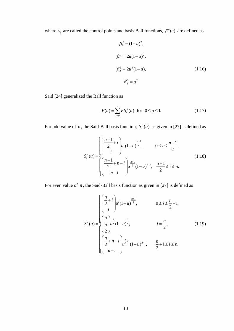
where iv are called the control points and basis Ball functions, ( )n
i u are defined as
3 2
0 (1 ) ,u
3 2
1 2 (1 ) ,u u
3 2
2 2 (1 ),u u (1.16)
3 2
3 u .
Said [24] generalized the Ball function as
0
( ) ( ) for 0 1.n
n
i i
i
P u v S u u
(1.17)
For odd value of n , the Said-Ball basis function, ( )n
iS u as given in [27] is defined as
1
2
1
2
11
(1 ) , 0 ,22
( )1
1(1 ) , .2
2
n
i
n
i
n
n i
ni n
u u i
iS u
nn i n
u u i n
n i
(1.18)
For even value of n , the Said-Ball basis function as given in [27] is defined as
1
2
2 2
12
(1 ) , 0 1,22
( ) (1 ) , ,2
2
(1 ) , 1 .22
n
i
n n
n
i
n
n i
ni n
u u i
i
nn
S u u u in
nn i n
u u i n
n i
(1.19)

11
It is obvious that when 3n , the cubic Said-Ball basis functions are
3 3
0 0 ,S
3 3
1 1 ,S
3 3
2 2 ,S (1.20)
3 3
3 3 ,S
as in (1.16).
Similarly, Wang-Ball curves [31] generalized a cubic Ball curve to higher degree
( 2)n and the Wang-Ball curve of degree n can be described as
0
( ) ( ) for 0 1,n
n
i i
i
P u vW u u
(1.21)
where
2
2 2
2 2
(2 ) (1 ) , 0 1,2
(2 ) (1 ) , = ,2
( )
(2(1 )) , = ,2
(1 ), .2
i i
n n
n
i n n
n
n i
nu u i
nu u i
W un
u u i
nW u i n
(1.22)
Again, when 3n , the cubic Wang-Ball basis functions , ( )n
iW u are
3 3
0 0 ,W
3 3
1 1 ,W
3 3
2 2 ,W (1.23)
3 3
3 3 ,W
as in (1.16).

12
Properties of Ball polynomials [24]
A Ball polynomial is defined in (1.15), (1.17) and (1.21) provided a number of
properties of Ball polynomials that lead to the properties of Ball curve.
(i) Positivity (Ball polynomials are non-negative)
( ) 0, ( ) 0, ( ) 0, [0,1].n n n
i i iu S u W u u
(ii) Partition of Unity
0 0 0
( ) 1, ( ) 1, ( ) 1, [0,1].n n n
n n n
i i i
i i i
u S u W u u
(iii) Symmetry
( ) (1 ), for 0,1,..., ,
( ) (1 ), for 0,1,..., ,
( ) (1 ), for 0,1,..., .
n n
n i i
n n
n i i
n n
n i i
u u i n
S u S u i n
W u W u i n
Properties of Ball curve [32]
In designing a curve, a Ball curve ( )P u of degree n has to satisfy the following
properties
(i) Endpoint Ball curve
The first control point of curve, 0P which starts at point 0u and last
control points of curve, 1P ends at point 1u such that
0 1(0) , (1) .P P P P
(ii) Endpoint Ball tangent
The tangent of Ball curve at the end points
1 0 1(0) ( ) and (1) ( ).n nP n P P P n P P

13
(iii) Convex hull property
When Ball curve iP satisfies the positivity and partion of unity properties
then the Ball curve iP lies in the convex hull of its control points.
(iv) Variation diminishing property
The number of intersection of a straight line (a plane) crosses Ball curve
iP not more than the number of intersection of the line (plane) crosses the
control polygon.
Rational Ball Curves
A rational Ball curve of degree n [29] can be defined as
0
0
( )
( ) , 0 1,
( )
nn
i i i
i
nn
i i
i
v w P u
B u u
w P u
(1.24)
where iv , iw , ( )n
iP u are respectively called the control points, weights and basis Ball
functions.
When 3n , the rational cubic Ball function can be expressed as
3 3 3 3
0 0 0 1 1 1 2 2 2 3 3 3
3 3 3 3
0 0 1 1 2 2 3 3
( ) ( ) ( ) ( )( ) .
( ) ( ) ( ) ( )
v w P u v w P u v w P u v w P uB u
w P u w P u w P u w P u
(1.25)
Specifically in this thesis, the generalized rational Ball function proposed by Tien
[29] has been applied in shape preserving curves and surfaces. The weights values
introduced into generalized Said-Ball functions causes Tien’s scheme to look a bit
different from Said-Ball functions. Rational Ball function is chosen because it has
shown less oscillation between interpolating points as compared to Ball polynomial
function, which has a tendency to oscillate due to its control point property of curve.

14
1.4 Continuity Conditions
In present day, CAGD has depending so much on mathematical descriptions of
objects based on parametric functions. A parametric spline function is piecewise
where each segments is a parametric function. An essential aspect of this function is
the way of the segment are joined together. The equations that control this joining are
called continuity constraints. Most applications in industrial design require
smoothness and shape fidelity. In CAGD, the continuity constraints are normally
chosen to get the given order of smoothness for the spline. The chosen order of
smoothness chosen is depends on the application. For examples, in mathematics
analysis field, the smoothness of function is measured by the number of continuous
derivatives and must has derivatives of all orders everywhere in its domain. Another
example is architectural drawing, where it is sufficient for the curves to be
continuous only in position. For design of mechanical parts, first and second order
smoothness are required [33].
In computer graphics, parametric continuity is the most frequently used in parametric
curves to describe the smoothness of the parameter values with distance along the
curve. Parametric continuity can be defined in nC notation which means it is until
the nth
order. Parametric continuity between two curves have same magnitude of the
derivative and parameter values. The following examples of two curves
0 1( ), ,P t t t t and 1 2( ), ,Q t t t t with order parametric continuity, nC satisfy [34]
1 1
1 1
1 1
1 1
( ) ( )
( ) ( )
( ) ( )
( ) ( )n n
P t Q t
P t Q t
P t Q t
P t Q t
In the above case, n is the order and 1t is the part where P and Q are joined.

15
Definition
A curve ( )s t is said to be nC continuous if the derivatives up to n
n
d s
dt are continuous
of value throughout the curve.
The idea of continuity ensures that curves and surfaces join together smoothly. The
various order of parametric continuity (smoothness) can be described as follows [34]:
0C continuity Curves are joined.
Only the end points are connected.
1C continuity Requires 0 C Continuity.
First-order derivatives are continuous.
The endpoints are connected and the tangents of both
curves have the same magnitude and direction at the
same parameter value.
2C continuity Requires 0C and 1C continuities.
Second-order derivatives are continuous.
Curvatures for both curves have the same magnitude and
direction.
1.5 Literature Review
In this section, the reviews are divided into two parts, which are curve and surface.
The discussion on the previous works are related with the field of shape preserving
of positivity, monoticity, convexity and constraint. First paragraph eloborates
reviews of shape preserving curve interpolation and the second paragraph discusses
the reviews on shape preserving surface interpolation.

16
1.5.1 Positivity Preserving Curve and Surface
Schmidt and Heb [35] derived the necessary and sufficient conditions for the positive
interpolation using cubic polynomial C1
spline. Since, the positive interpolants had
not determined uniquely, so the geometric curvature had minimized if one of them
selected. In contrast, Hermite piecewise cubic interpolant [36] has been used to solve
the problem of interpolating C1 positive in the sense of positivity schemes and even
though it is very economical, the method generally inserted extra knots in the interval
to visualize and conserves the shape of data. The proposed scheme described in [37]
used C1 piecewise rational cubic Hermite spline did not offer shape parameters
which played a role as free parameter to modify positive curve if needed. Sarfraz et
al. [11] constructed a rational cubic Bézier interpolant with two families of shape
parameters to obtain C1 positivity or monotonicity preserving spline curves. Sarfraz
[38] extended the scheme in [11] which used rational cubic Bézier with two families
of shape parameters to preserve the shape of positivity and convexity data. As a
result the scheme produced C1 interpolant. Zheng et al. [39] tried to solve the
problems of positive and convex polynomials. They suggested the problem of
convexity polynomials could be solved by using positivity, where in algorithm Sturm
of positive polynomials they used the extended classic Sturm theorem. The reason of
positivity polynomial choice was the proof of similarity between convexity of
polynomial and the positivity of its second order derivative within the same interval.
Goodman [40] discussed the problem of curve preservation through a finite sequence
of points. He suggested algorithms were able to preserve the shape of data. Asim and
Brodlie [41] had developed the scheme of piecewise cubic Hermite interpolant that
conserved the positivity of positive data by added one additional point within the
interval of the positivity lost interpolant. The scheme improved the algorithm in [42]

17
which inserted two additional points within the interval. Duan et.al [43] developed
new method to create higher-order smoothness interpolation. They used certain
function values on rational cubic Bézier interpolation to manage the shape of data.
Brodlie et al. [44] discussed the issue of positive data visualization and they
developed a scheme with interpolated scattered data using dimension Modified
Quadratic Shepard method. The scheme made the quadratic basis function became
positive and automatically preserved the positivity. The method continued to
preserve interpolant that lay between any two specified functions as lower and upper
bounds. While in Hussain and Ali [45] study, they established a piecewise rational
cubic Bézier function with two shape parameters which can preserved the shape of
positive data. The scheme did not provide free parameters to adjust shape of positive
curve. Even though the scheme lacked with adjustability, the curve visual seem
smooth and achieved C1 continuous curve. Whereas Hussain and Sarfraz [46] used
rational cubic Bézier function proposed in [37] and extended to rational bicubic
Bézier form. The rational cubic Bézier function involved four shape parameters
where two parameters assumed as constrained parameters to preserve positive data
in the form of positivity curve. While the other two gave freedom to adjust the curve.
Hussain et al. [47] discussed the problem of the shape preserving C1 rational cubic
Bézier interpolation and they developed the function that had only one free
parameter to preserve the shape of data, but unprovided flexible parameter for users
to refine the curve. Study by Sarfraz et al. [42] produced a rational cubic Bézier
function with two parameters. This function used to visualize 2D positive data. They
produced C1 interpolant and no additional points inserted. They also extended the
scheme to rational bi-cubic Bézier partially blended with purposed to visualize the
shape of 3D data. While Sarfraz et al. [48] built up a piecewise rational Bézier

18
function with cubic numerator and cubic denominator scheme which involved four
shape parameters in each subinterval. Two shape parameters preserved the curves
and the other two parameters free for modification of positivity, convexity and
constraint curves. From this, data dependent constraints derived with the degree of
smoothness C2. The scheme did not offer flexibility parameters for adjusted the
shape of positive, monotone and convex data. In another study, Sarfraz et al. [16]
considered the piecewise rational cubic Bézier spline interpolation into positive,
monotone and convex data. They introduced four shape parameters used in the
rational interpolation. The calculated error of interpolating rational cubic scheme was
order 3( )O h . Some rational cubic spline functions based on Bernstein-Bézier basis
function in the form of (cubic numerator and cubic denominator) [49, 50] with
developed shape parameters to visualize the 2D positive data. These rational cubic
Bézier schemes had common characteristics in term of C1 and C
2 continuities, local
and no extra knots inserted in the interval of interpolants that lost the inherited shape
features. Sarfraz et al. [49] discussed two objectives; first objective developed new
interpolation scheme using rational cubic Bézier function and second objective used
the generated scheme in application. The authors also addressed the problem of
visualization for positive, monotone, convex and constrained data. Studies by Karim
[50] explained the preservation of positivity using rational cubic Bézier spline and
proposed GC1 cubic interpolant with two shape parameters. Then Karim and Kong
[51] constructed new C2 rational cubic Bézier spline interpolant with cubic
numerator and quadratic denominator. The new proposed scheme which extended to
preserve positive data had three parameters, where one parameter was sufficient
condition and two parameters were set free for users to change the final shape of
curves.

19
Schmidt et al. [52] discussed the positive interpolation using rational quadratic
splines. They constructed necessary and sufficient conditions under the property of
positivity. Butt [53] interpolated positive data with bicubic function. The study
generated necessary and sufficient conditions based on the first partial derivatives to
preserve the positivity data. While Schmidt and Dresden [54] studied shape
preservation of positive, monotone and S-convex data given on rectangular grids.
They derived scheme based on C1 rational biquadratic splines [55]. Brodlie et al. [56]
solved the problem of shape preserving and visualized positive data by introducing
piecewise cubic Hermite interpolant. The shape of surface required to preserve the
positivity of positive data. Both first order partial derivatives and mixed partial
derivatives need to provide under the case of rectangular grid. The scheme also
inserted one or more than two extra points. Then, Casciola and Romani [57]
proposed bivariate scheme based NURBS (Non-uniform rational basis spline) to
preserve the shape of surface data by using tension parameters. The scheme
technique was based on conversion from proposed technique discussed in [58, 59].
Hussain and Hussain [59] expanded the rational cubic Bézier function with cubic
numerator and quadratic denominator to rational bicubic Bézier partially blended
function (Coons patch). Simple constraints developed on free parameters in the
description of rational cubic Bézier and rational bicubic Bézier function to visualize
positive data. In another study, Hussain and Hussain [60] used rational bi-cubic
Bézier spline based on rational cubic Bézier with cubic numerator dan cubic
denominator [61] and solved the problem of shape preservation of positive surface
data and also for the one that lay above the plane. Then Safraz et al. [42] used a
rational cubic Bézier function and considered two shape parameters to preserve the
shape of curve positive data. They also extended the rational cubic Bézier function to

20
rational bi-cubic Bézier partially blended function and considered simple data
dependent constraints to preserve the inherited shape feature of 3D positive data. In
the scheme, the shape of curves and surfaces of positive data cannot be modify
because the interpolant did not has free parameter. Meanwhile, Hussain et al. [62]
developed surface scheme for positive and convex data using rational bi-quadratic
Bézier spline function. They proved that the developed scheme was economically
computation and pleasantly visual. Then, Abbas et al. developed a rational bi-cubic
Bézier function [63, 64] which an extended form of cubic numerator and quadratic
denominator with three shape parameters and also constructed rational bi-cubic
Bézier partially blended (Coons patches) [65, 66] functions with twelve shape
parameters to solve the problem of positivity preserving surface through positive data
by imposing simple conditions on shape parameters. Study by Hussain et al. [64]
presented local interpolation scheme using C1 rational bi-cubic Bézier function. The
surface scheme provided eight shape parameters in rectangular patch to preserve
positive, monotone and convex surface data. Liu et al. [65] constructed the biquartic
rational interpolation spline for surface over the rectangular domain, which included
the classical bicubic Coons as a special case. The sufficient conditions generated for
positive or monotone surface data. Hussain et al. [67] used C1 Bézier-like bivariate
rational interpolant to preserve positive and monotone surface data. The scheme
generated eight shape parameters in each rectangular patch. Data dependent
constraints developed on four of these free parameters to preserve the positive and
monotone surface data. The rest of four parameters used for shape refinement. In
another study Hussain et al. [68] developed alternate scheme to conserve positive and
monotone regular surface data. The alternate scheme used GC1 bi-quadratic
trigonometric function and generated four constrained shape parameters in each

21
rectangular patch to avoid unnecessary oscillations in positive and monotone
surfaces data. Karim et al. [69] discussed the problem of positivity preserving for
positive surfaces. They used C1 rational cubic Bézier spline and extended to C
1
bivariate cases. They proved that proposed scheme, partially blended rational bicubic
Bézier spline with twelve parameters was on par with the established methods based
on the results of Root Mean Square Error (RMSE).
1.5.2 Monotonicity Preserving Curve and Surface
McAllister et al. [70] proposed algorithm that used polynomial Bézier function to
preserve monotonicity and convexity. While Schumaker [71] dealt with the
algorithm for interpolating discrete data. An algorithm used C1 Hermite quadratic
splines, which flexible to preserve the monotone or convex data. Delbourgo and
Gregory [72] dealt with the problem of shape preserving interpolation for convex and
monotone data. They used C1 piecewise rational cubic Bézier included the rational
function for quadratic preserving and calculated the error analysis which was 4( )O h .
Study by Costantini [73] used Bernstein polynomials to interpolate spline of
monotone and convex with suitable continuous piecewise linear function. Then, Lam
[74] discussed the method of preserving monotone and convex discrete data. The
study used function which was quadratic Bézier spline proposed by Larry Schumaker
[71]. The basic idea behind the spline was the value of first order derivatives
selection at the given data points. Fiorot and Tabka [75] expressed C2 cubic
polynomial interpolation Bézier spline in condition of the existence or nonexistence
of solutions for a system of linear inequalities with two unknowns. The proposed
method focused on shape preserving convex or monotonic data. Then, Shrivastava
and Joseph [76] considered C1-piecewise rational cubic spline function which

22
involved tension shape parameters. The method used to preserve monotonic data and
under certain conditions to preserve convex data. The error analysis of the interpolant
was calculated. Lamberti and Manni [77] discussed a method for construction of
shape preserving C2 function interpolating based on parametric cubic Hermite curve.
The constructed scheme used tension shape parameters, which had an immediate
geometric interpolation to control the shape of positivity, monotonicity and
convexity curve. Wang and Tan [78], constructed rational quartic Bézier spline
function (quartic numerator and linear denominator) and two parameters to construct
monotonic interpolant. The curve reached C2 continuity and error analysis of the
interpolant was calculated. Goodman and Ong [79] presented a local subdivision
scheme based on B-spline function. The scheme worked with uniform knots to assure
the shape of data was local, monotonicity and convexity. Jeok and Ong [80] studied
the usage of cubic Bézier-like in preserving monotonicity interpolation and
constrained interpolation. The cubic Bézier-like was extended function of cubic
Bézier polynomial functions where, the cubic Bézier polynomial scheme inserted
two additional parameters to modify curve. Based on this function, two interpolation
schemes were constructed. The first interpolation scheme generated C1 monotonicity
preserving curves while the second generated G1 curve which were constrained to lie
on the same of the given constraint lines as the data. Hussain and Sarfraz [12] solved
the problem of monotonicity. The scheme used C1 piecewise rational cubic Bézier
function with four free parameters over the interval to preserve the monotonicity of
monotone data. The scheme gave opportunity for users to amend the curve
interactively. A study by Tian [81] represented C1 piecewise rational cubic Bézier
spline with quadratic denominator to generate monotonic interpolant. The error
analysis provided and the results showed the stable interpolant. Abbas et al. [82]

23
discussed visualization of monotone data with C1 continuity smoothness. They used
rational cubic Bezier function with three shape parameters in each interval. The
conditions provided freedom for users to generate pleasant curve interactively.
Studies by Piah and Unsworth [83] improved sufficient conditions generated in [78].
The proposed scheme improved sufficient conditions based on rational Bézier quintic
function (quartic numerator and linear denominator), improved monotonicity region
and ensured the monotonicity of data. The improved scheme presented C2 continuity
and local. Cripps and Hussain [84] constructed a piecewise monotonic interpolant.
According to rational cubic Bézier univariate function, they derived the free
parameters for users in term of weights function. The generated sufficient conditions
used to preserve monotonicity. Abbas et al. [85] suggested rational cubic Bézier
function with three shape parameters and one of them used to preserve the inherited
shape feature of monotone curve. The other two remained for refining the aim shape
of monotone curve as desired. Sun et al. [86] presented weighted rational cubic
Bézier spline with linear denominator. The scheme achieved the degree of
smoothness C2 and handy to preserve shape of monotone and convex data by
choosing the parameters properly. Then, Wang et al. [87] constructed weighted
rational quartic Bézier spline interpolation based on two types of rational quartic
Bézier spline with linear denominator. The conditions preserved monotonicity and
achieved C2 continuity. While Karim [88] studied the problem of monotonicity
preserving GC1
interpolation. The scheme used Ball cubic interpolant and derived
necessary, sufficient conditions and unneeded any derivative modified for controlling
the shape of monotonic interpolate curve.
Fritsch and Carlson [89] extended the method in [90] to bicubic interpolation on
rectangular mesh. The Hermite function used to produce the derivatives based on

24
five step procedures that ensured monotonic interpolant. Beatson and Ziegler [91],
analyzed C1 monotone data using quadratic splines and proposed an algorithm for
interpolating monotone data in rectangular grid and error analysis was provided.
While Carlson and Fritsch [92] discussed an algorithm for monotone interpolation of
monotone data in rectangular mesh. They used bicubic Hermite functions to develop
conditions on the derivatives, then they were ample to make the functions became
monotonic. A study by Costantini and Fontanella [93] presented a method for
surfaces preservation on rectangular grids. They introduced a surface that was a
tensor product from Bézier splines of arbitrary continuity class which extended from
[73]. Sarfraz et al. [94] developed C1 monotonicity shape preserving scheme. The
scheme used rational cubic Bézier functions (cubic numerator and quadratic
denominator) with three shape parameters. The scheme automatically converted
higher degree of the interval to lower degree effectively according to the nature of
the slope and parameters in that interval. For monotone data visualization, Hussain
and Hussain [13] used rational cubic Bézier function proposed in [95]. The function
applied to partially blended rational bicubic Bézier function (Coons patches) to
visualize monotone surface data. Delgado and Pena [96] introduced Ball basis for
cubic polynomials. Two types of generalization called Said-Ball basis and Wang-
Ball basis were constructed for polynomials in high degree m. They proved that the
Wang-Ball basis only preserved monotonicity for all m but unpreserved geometric
convexity and not totally positive for 3m , in contrast from Said-Ball basis.
Delagado and Pena [97] proved that rational Bézier surfaces did not preserve
monotonicity axially, and the surfaces that were generated by the tensor product of
rational Benstein basis also did not preserve monotonicity. Tian [98] developed a C1
piecewise rational cubic Bézier spline with quadratic denominator to preserve