Visual Psychophysics and Physiological Optics · Visual Psychophysics and Physiological Optics Spatial Entropy Pursuit for Fast and Accurate Perimetry Testing Derk Wild, Sxerife Seda

Visual Psychophysics and Physiological Optics

Spatial Entropy Pursuit for Fast and Accurate PerimetryTesting

Derk Wild, Sxerife Seda Kucur, and Raphael Sznitman

Ophthalmic Technology Laboratory, ARTORG Center for Biomedical Engineering Research, University of Bern, Bern, Switzerland

Correspondence: Raphael Sznitman,Ophthalmic Technology Laboratory,ARTORG Center for Biomedical En-gineering Research, University ofBern, Murtenstrasse 50, CH-3008,Bern, Switzerland;[email protected].

Submitted: November 19, 2016Accepted: May 22, 2017

Citation: Wild D, Kucur SxS, SznitmanR. Spatial entropy pursuit for fast andaccurate perimetry testing. Invest

Ophthalmol Vis Sci. 2017;58:3414–3424. DOI:10.1167/iovs.16-21144

PURPOSE. To propose a static automated perimetry strategy that increases the speed of visualfield (VF) evaluation while retaining threshold estimate accuracy.

METHODS. We propose a novel algorithm, spatial entropy pursuit (SEP), which evaluatesindividual locations by using zippy estimation by sequential testing (ZEST) but additionallyuses neighboring locations to estimate the sensitivity of related locations. We model the VFwith a conditional random field (CRF) where each node represents a location estimate thatdepends on itself as well as its neighbors. Tested locations are randomly selected from a poolof locations and new locations are added such that they maximally reduce the uncertaintyover the entire VF. When no location can further reduce the uncertainty significantly,remaining locations are estimated from the CRF directly.

RESULTS. SEP was evaluated and compared to tendency-oriented strategy, ZEST, and theDynamic Test Strategy by using computer simulations on a test set of 245 healthy and 172glaucomatous VFs. For glaucomatous VFs, root-mean-square error (RMSE) of SEP wascomparable to that of existing strategies (3.4 dB), whereas the number of stimuluspresentations of SEP was up to 23% lower than that of other methods. For healthy VFs, SEPhad an RMSE comparable to evaluated methods (3.1 dB) but required 55% fewer stimuluspresentations.

CONCLUSIONS. When compared to existing methods, SEP showed improved performances,especially with respect to test speed. Thus, it represents an interesting alternative to existingstrategies.

Keywords: static perimetry, perimetry testing, machine learning

Given its long history, visual field estimation by perimetryexamination remains a standard approach for detection

and monitoring of visual impairment. Static white-on-whiteautomated perimetry (SAP) is perhaps the most common formand has been paramount for large clinical studies measuringvisual function for glaucomatous patients1,2 and patients withneurological disorders.3

At the heart of SAP lies a sequential light-stimulus andpatient response exchange to estimate local ‘‘sensitivitythresholds’’ at specific locations of the visual field, that is, theamount of light stimulus that would induce a 50% chance ofbeing identified by a subject. Typically used to measure thecentral 248 to 308 of the visual field, presenting all possiblestimulus intensities at all locations, multiple times, would allowa highly accurate estimation of the complete visual field.Unfortunately, such a strategy would be desperately slow andexhausting for the subject. Conversely, presenting a singlestimulus to estimate a handful of locations would be fast buthighly inaccurate. As such, perimetry strategies implicitly sufferfrom an accuracy-speed trade-off, where the ideal goal is to beboth fast and accurate.

Given this fact, numerous strategies have been proposedwith most strategies falling into one of two groups: (1) thoseestimating location sensitivity independently of other loca-tions4,5 and (2) those who use neighboring locations toestimate sensitivity of related locations.6–8 The latter category

has received growing interest as it appears to optimize speedand accuracy more effectively.

Most notably, the dynamic test strategy6 uses a dynamicapproach to estimate thresholds at locations and leveragesfound location values to seed neighboring locations whenselected for testing. Alternatively, tendency-oriented strategy(TOP)8,9 uses neighboring locations to estimate sensitivitythresholds in an asynchronous fashion, leading to extremelyfast estimation at the cost of accuracy. More recently, newstrategies10,11 have focused on using neighboring locations in amore data-driven and coherent fashion, which has led toimproved performances. Our work follows this line of researchas well.

In an effort to further improve perimetry accuracy andspeed, we propose in this work an alternative strategy, namely,spatial entropy pursuit (SEP). Our underlying idea is that visualfields should be estimated in a global fashion, where final andintermediate results at different locations can be used toestimate other locations. SEP follows a standard perimetrystrategy for individual locations (i.e., zippy estimation bysequential testing [ZEST]) and begins by measuring fourlocations. Our approach then attempts to locate whichlocations should be tested next in order to provide the largestinformation gain with respect to the uncertainty of the entirefield. The testing procedure can then be stopped when theoverall uncertainty has attained a user-specified level and thusavoids the need to test all locations. In practice, we model the

Copyright 2017 The Authors

iovs.arvojournals.org j ISSN: 1552-5783 3414

This work is licensed under a Creative Commons Attribution-NonCommercial-NoDerivatives 4.0 International License.

Downloaded From: http://iovs.arvojournals.org/pdfaccess.ashx?url=/data/journals/iovs/936360/ on 07/17/2017

source: https://doi.org/10.7892/boris.102085 | downloaded: 16.6.2020

https://creativecommons.org/licenses/by-nc-nd/4.0/

visual field as a large conditional random field (CRF)12

represented as a graph of location estimates whose valuesdepend on themselves as well as on their neighbors. Priorlocation estimates as well as neighborhood relationships arederived from a large data set of glaucomatous visual fields. Forcomparison, we evaluated the performance of our methodagainst that of existing strategies by using simulationsimplemented in the open perimetry interface (OPI).13

METHODS

To reduce perimetry examination duration without compro-mising accuracy, we made use of the spatial relationships be-tween neighboring visual field locations as previouslysuggested by Chong et al.10 and Rubinstein et al.11 Accordingly,an iterative scheme was derived that follows ZEST testing5 atindividual locations and internally determines the next locationand stimulus intensity to use by leveraging a visual field model.We begin by explaining our method and the visual field modeland how we evaluated our algorithm by using computersimulations.

ZEST Strategy

Briefly, in ZEST, each visual field location is associated with aprior probability mass function (PMF), which represents theprobability of a given sensitivity threshold. ZEST then (1)selects a visual field location randomly from a pool containingall unfinished locations and (2) presents one light stimuluswith the stimulus intensity at the mean of the PMF at theselected location; (3) the subject response is incorporated intothe PMF in a Bayesian way by multiplying the likelihoodfunction (i.e., probability-of-seeing curve) for the givenresponse with the PMF. Steps (1) to (3) are then repeateduntil the stopping criterion is reached (i.e., the uncertainty ofthe PMF, measured by the Shannon entropy,14 is lower than apredefined value), at which point the location is removed fromthe pool of unfinished locations. ZEST terminates when alllocations have been tested.

To generate the initial PMFs of the visual field locations, weused visual field data of glaucomatous patients from theRotterdam Ophthalmic Institute’s ‘‘Longitudinal GlaucomatousVisual Field data’’1,15 (4863 visual fields from 278 eyes of 139glaucoma patients). To generate smooth PMFs from these data,the PMFs were smoothed by using a Gaussian kernel (r¼ 1.5,window ¼ 10 dB).

Visual Field Model

To infer sensitivity threshold probabilities (i.e., PMFs) for visualfield locations from neighboring locations, we used a CRF. Inour CRF, a node describes a visual field location and nodes areconnected by edges that represent the probabilistic relation-ships between locations. In this work, we modeled the 24-2test pattern and assumed that each location (except the ones atthe border of the test pattern) has a four-neighborhoodconnection, as depicted in Figure 1a. Each node correspondsto a PMF representing a visual field location sensitivitythreshold probability, and edges are PMFs that encode theconditional probability distributions for pairs of thresholdsensitivities (Figs. 1b–d). The edge PMFs are generated fromthe data and smoothed with a Gaussian kernel (r ¼ 2.5,window ¼ 10 dB 3 10 dB).

To compute estimates for the unfinished locations we usedthe Loopy Belief Propagation method,16 which propagatesinformation found at individual locations to neighboring nodesiteratively and leverages the spatial relationships of locations

encoded via edge connections. In this way, each nodeinfluences nodes further away according to probabilisticdependencies. To avoid updating the nodes corresponding toalready finished locations, we fixed these nodes’ PMFs duringthe information propagation.

Note that we used a four-neighborhood connection tomodel location interactions in this work. While simple, otherspatial configurations such as retinal nerve fiber layer-inspiredconnections as described by Jansonius et al.,17,18 could be usedinstead.

The SEP Algorithm

The proposed SEP algorithm is an algorithm that uses theZEST method at given locations but differs in the way thelocations to be tested are selected. In particular, we make useof a pool of four locations that are being tested at any givenpoint in time and which are initially selected as those withhighest uncertainty according to their initial PMF. Thealgorithm then automatically and dynamically removesterminated locations from this pool and adds new locationsin a way that reduces the overall uncertainty of the visual fieldas much as possible.

In practice, at each stimuli presentation, one of fourlocations in the pool is selected randomly and tested by usingZEST as described above. This is done until one of the fourlocations finishes, at which point it is removed from the pool.A new location is then added in the following way: (1) thecurrent PMFs of all locations are placed into the visual fieldmodel; (2) the visual field model is then used to approximatethe most likely PMF for each unfinished location as based onall responses over all locations; and (3) PMFs are then used toselect the most informative location among the untestedlocations. To do this we define a function that is computed foreach untested location and that combines two measures,namely, the Shannon entropy of the location estimate and itsneighborhood heterogeneity,

Ci ¼ MH ið Þ þ aMG ið Þ; ð1Þwhere MH (i) and MG(i) are nonnegative and stand for theentropy and neighborhood heterogeneity of the visual fieldestimates at location i, respectively. The parameter a � Rþ is aweight that influences the relative importance of these twofactors. The next location is then selected as the onemaximizing Ci in Equation 1, implying that either one orboth of the defined measures should be high. The entropymeasure, MH (i), quantifies the uncertainty of the modeledPMF of location i, while the neighborhood heterogeneity,MG(i), represents an approximation of the spatial thresholdgradient of the current field estimate (see Appendix A forcomputational details). In particular, MG(i) quantifies neigh-borhood threshold consistency and is higher at locationswhose neighbor estimates differ from one another.

Note that Equation 1 implicitly presumes that poorneighborhood consistency is a good indicator to test. Oncethe location with the highest Ci is moved to the pool oflocations to be tested, we substitute the PMF of the newlyadded location with that of the modeled PMF. This is achievedby summing the model PMF with a constant d, to reduce itsconfidence, and then multiplying it with the prior PMF. Thiseffectively avoids being overconfident in the model probabil-ities.

With four locations in the pool again, the procedure restartsand continues until Ci is lower than a predefined value. In thiscase, no additional location is moved to the pool and thealgorithm terminates as soon as the remaining three locationsare finished. Importantly, this implies that SEP does not

Spatial Entropy Pursuit IOVS j July 2017 j Vol. 58 j No. 9 j 3415


measure all visual field locations and infers sensitivitythresholds for the untested locations from the visual fieldmodel after termination of the algorithm.

Evaluation of SEP

Our algorithm was implemented and evaluated by means ofcomputer simulations using the R package OPI.13 Responses tostimuli presentations were modeled by sampling from aFrequency-of-Seeing (FOS) curve (i.e., psychometric function)with a predefined false-positive and false-negative responserate of 3% and 1%, respectively. The slope of the FOS curve fora given threshold was modeled with a cumulative normaldistribution with standard deviation (SD) according to apublished variability formula.19 The maximum standarddeviation allowed for the slope was set to 6 dB. To findsuitable parameters for SEP and ZEST (i.e., parameters thatminimize the number of stimulus presentations while yieldingaccuracy levels comparable to the dynamic test strategy), aparameter optimization procedure was performed (see Appen-dix B) on a subset of the data.

To evaluate SEP’s performance in terms of accuracy andtesting duration (i.e., number of stimulus presentations), wecompared it to ZEST, TOP,20 and the Haag-Streit dynamic test

strategy, which we denote as ZEST, TOP-like, and dynamic-like,respectively (exact implementations of dynamic test strategyand TOP are not public and may slightly differ from ourimplementation).

To compare methods, simulations were performed by usinga test set with visual fields of 10 randomly selectedglaucomatous eyes from the data (on average 17 visual fieldsper eye [SD¼ 2.2]), whereby all visual fields of the selected 10eyes were removed from the data used to generate prior PMFsand edge potentials. Simulations with glaucomatous eyes wereperformed five times with different test sets, in order to controlfor selection bias (see Appendix C). In addition, to assessperformance for healthy patients, simulations were performedon 245 healthy visual fields (Mean MD ¼ 0.021 dB, SD ¼ 1.7)from the Rotterdam Ophthalmic Institute (control data fromthe data). Each visual field was measured five times to gathertest–retest variability.

To quantify the accuracy of an algorithm, we made use ofthe RMSE between the true and estimated sensitivity thresholdat all locations in a visual field. We also examined how SEPperforms on scotoma regions by checking the estimationerrors at locations with a high scotoma measure as defined byRubinstein et al.11 Here we computed maxd, by calculating thegreatest difference in threshold sensitivity between a location

FIGURE 1. Conditional random field model. (a) The graph used for our visual field model (24-2 test pattern). (b) Prior probability mass function oflocation 20. Bars represent the raw PMF, the line represents the smoothed PMF. (c) Raw PMF for the edge connecting locations 20 and 21. (d)Smoothed PMF for the same edge.



FIGURE 2. Example visual field measurement with SEP. The top figure represents the glaucomatous visual field that was measured (MD¼�11.8 dB).For each stage, that is, stimulus presentation, the figure on the left represents the current visual field estimate and the figure on the right shows thenumber and locations of presented stimuli. Black boxes indicate finished locations.



and any of its eight adjacent locations (ignoring the blind spotlocations 26 and 35). Thus, high maxd values indicate locationsat scotoma borders, whereas low values indicate locations inuniform regions.

RESULTS

To provide a qualitative understanding of SEP, Figure 2 depictsthe order in which different locations were selected fortesting and the associated estimated visual field as function ofpresented stimuli for a given example. In this example, aglaucomatous visual field with an MD of�11.8 dB was testedwith SEP, and the estimated visual field at intervals of stimuluspresentations is shown. SEP concluded after 131 presenta-tions, and 11 visual field locations were inferred in thisexample.

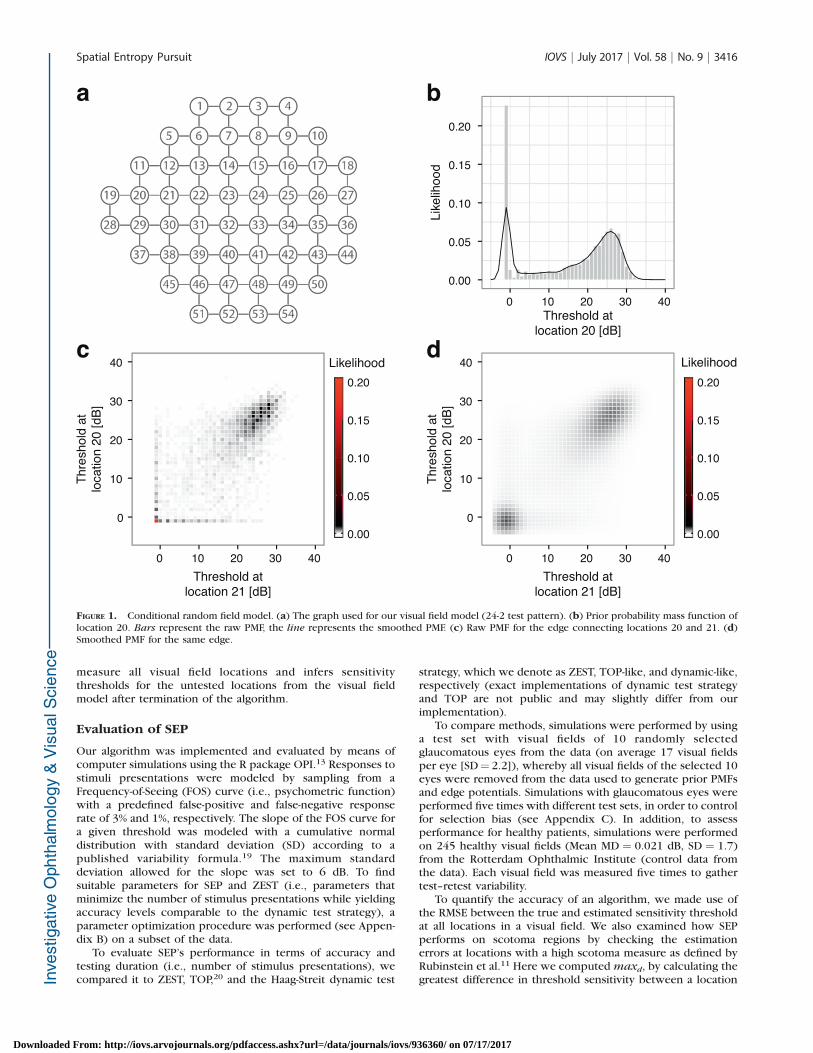
For 245 healthy visual fields, the simulation result isdisplayed in Figures 3a and 3c. The median RMSE of the testedvisual fields was 3.1 dB in both SEP and ZEST (nonsignificantdifferences, Mann-Whitney U test, P > 0.05). Median RMSE inthe dynamic-like strategy was 2.3 dB (significant differencewith SEP, Mann-Whitney U test, P < 0.001). The mediannumber of stimulus presentations was 64 in SEP, 98 in ZEST,and 142 in the dynamic-like strategy (significant differences,

Mann-Whitney U test, P < 0.001). The TOP-like strategy hadsignificantly lower number of stimulus presentations than allother algorithms, but also significantly higher median RMSE of4.8 dB (Mann-Whitney U test, P < 0.001).

Similarly, Figures 3b and 3d report the performances ofeach method on glaucomatous visual fields (one test set isshown). In this plot the test set contains a total of 172 visualfields from 10 eyes, acquired over an average time span of 8.9years (SD¼ 1.1). The average MD of the visual fields is�10 dB(SD ¼ 7.8). The median RMSE was 3.4 dB in both SEP andZEST (nonsignificant differences, Mann-Whitney U test, P >0.05) and 3.5 dB in the dynamic-like strategy (significantdifference with SEP, Mann-Whitney U test, P < 0.01). Themedian number of stimulus presentations was 113 in SEP, 123in ZEST, and 146 in the dynamic-like strategy (significantdifference, Mann-Whitney U test, P < 0.001). The TOP-likestrategy has significantly lower number of stimulus presenta-tions than the other algorithms, but also significantly highermedian RMSE of 5.8 dB (Mann-Whitney U test, P < 0.001). InSEP, there is no clear dependency of RMSE on MD whereasnumber of stimulus presentations correlates well with MDespecially for MD values between 0 and�14. This is expectedas SEP was optimized as to provide the same accuracy levelfor any subject by adapting its speed. The relationship

FIGURE 3. Performance of SEP compared to existing methods. Number of stimulus presentations and root-mean-square error of visual fieldsmeasured with SEP, ZEST, dynamic-like, and TOP-like strategies. Each visual field was tested five times. (a–c) Simulations performed with 245 healthyvisual fields (MD ranging from�6.4 to 3.2 dB). (b–d) Simulations performed with 172 glaucomatous visual fields (MD ranging from�31.1 to 5.1 dB).



between RMSE and MD however reveals that the median erroris highest in visual fields with intermediate MD of �14,corresponding mostly to heterogeneous visual fields (seeAppendix D).

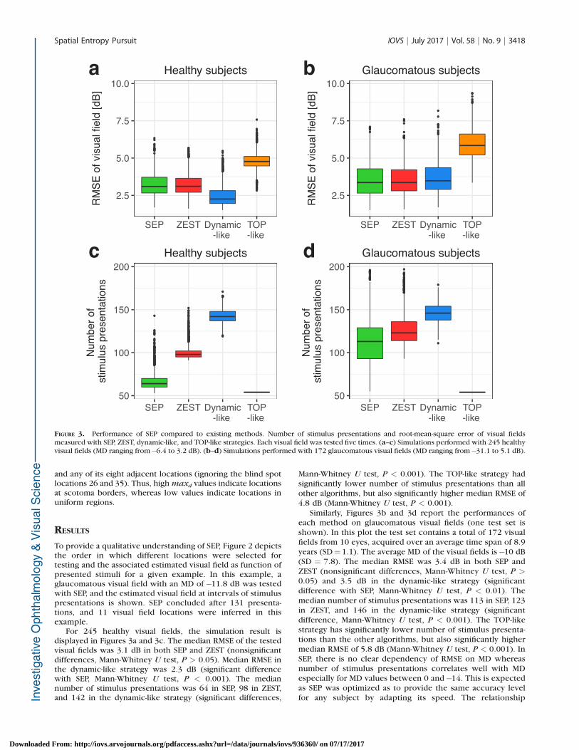
Figure 4 reports the distributions of the pooled errors overall locations and visual fields. The error bias, that is, meanerror, was�0.11 dB (SD¼ 6) in TOP, 0.17 dB (SD¼ 3.7) in SEP,0.28 dB (SD ¼ 3.7) in ZEST, and �0.69 dB (SD ¼ 3.8) in thedynamic-like strategy. The distributions differed significantlybetween algorithms (two-sample t-test, P < 0.05). Absolutemean error of tested locations of SEP was 0.23 dB (SD ¼ 3.3),compared to that of untested locations, which was�0.0016 dB(SD ¼ 4.5). The distributions between tested and untestedlocations of SEP differed significantly (two-sample t-test, P <0.001). The average number of tested locations per visual fieldin SEP was 39 (SD ¼ 5.1) out of 54.

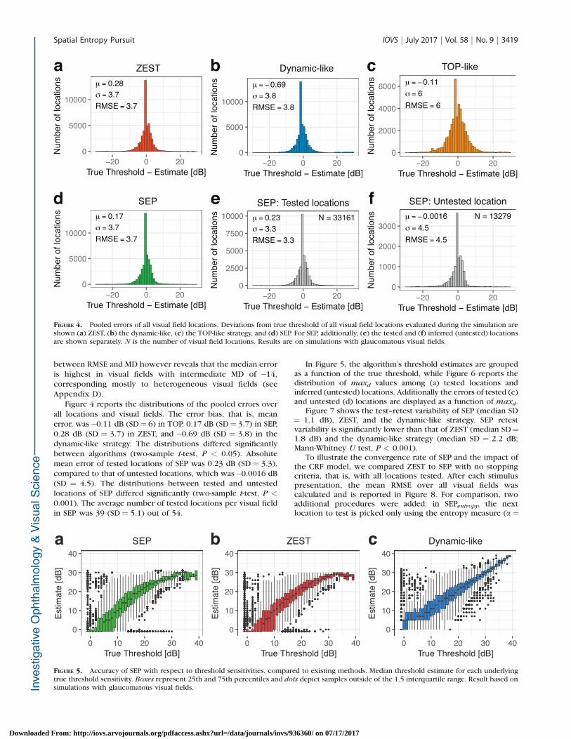
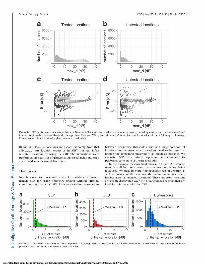
In Figure 5, the algorithm’s threshold estimates are groupedas a function of the true threshold, while Figure 6 reports thedistribution of maxd values among (a) tested locations andinferred (untested) locations. Additionally the errors of tested (c)and untested (d) locations are displayed as a function of maxd.

Figure 7 shows the test–retest variability of SEP (median SD¼ 1.1 dB), ZEST, and the dynamic-like strategy. SEP retestvariability is significantly lower than that of ZEST (median SD¼1.8 dB) and the dynamic-like strategy (median SD ¼ 2.2 dB;Mann-Whitney U test, P < 0.001).

To illustrate the convergence rate of SEP and the impact ofthe CRF model, we compared ZEST to SEP with no stoppingcriteria, that is, with all locations tested. After each stimuluspresentation, the mean RMSE over all visual fields wascalculated and is reported in Figure 8. For comparison, twoadditional procedures were added: in SEPentropy, the nextlocation to test is picked only using the entropy measure (a¼

FIGURE 4. Pooled errors of all visual field locations. Deviations from true threshold of all visual field locations evaluated during the simulation areshown (a) ZEST, (b) the dynamic-like, (c) the TOP-like strategy, and (d) SEP. For SEP, additionally, (e) the tested and (f) inferred (untested) locationsare shown separately. N is the number of visual field locations. Results are on simulations with glaucomatous visual fields.

FIGURE 5. Accuracy of SEP with respect to threshold sensitivities, compared to existing methods. Median threshold estimate for each underlyingtrue threshold sensitivity. Boxes represent 25th and 75th percentiles and dots depict samples outside of the 1.5 interquartile range. Result based onsimulations with glaucomatous visual fields.



0) and in SEPrandom, locations are picked randomly. Note thatSEPrandom tests location orders as in ZEST but still infersuntested locations by using the CRF. The simulations wereperformed on a test set of glaucomatous visual fields and eachvisual field was measured five times.

DISCUSSION

In this work, we presented a novel data-driven approach,namely SEP, for faster perimetry testing without stronglycompromising accuracy. SEP leverages existing correlations

between sensitivity thresholds within a neighborhood oflocations and assesses which locations need to be tested toreduce the remaining uncertainty as much as possible. Weevaluated SEP on a mixed population and compared itsperformance to state-of-the-art methods.

In the example measurement shown in Figure 2, it can beseen that all locations along the scotoma border are beingmeasured, whereas in more homogeneous regions, within aswell as outside of the scotoma, the measurement is coarser,leaving gaps of untested locations. These untested locationsare evenly distributed over the homogeneous regions that areideal for inference with the CRF.

FIGURE 6. SEP performance at scotoma borders. Number of locations and median measurement error grouped by maxd value for tested (a–c) andinferred (untested) locations (b–d). Boxes represent 25th and 75th percentiles and dots depict samples outside of the 1.5 interquartile range.Results are on simulations with glaucomatous visual fields.

FIGURE 7. Test–retest variability of SEP compared to existing methods. Histograms of standard deviations of estimates for the same location arepresented for SEP, ZEST, and dynamic-like strategies.



Simulations based on data from healthy patients show thatSEP can reduce the number of stimuli presentations by 35%when compared to ZEST and by 55% when compared to thedynamic-like strategy (Fig. 3a). While SEP and ZEST roughlyhave the same accuracy level, the dynamic-like strategy ismore accurate for healthy visual fields. SEP and ZEST, how-ever, are still more accurate than any of the tested algorithmswhen measuring glaucomatous visual fields. With a mediannumber of stimulus presentations of 64, SEP is almost as fastas the TOP-like algorithm for healthy visual fields, whilehaving much lower RMSE. On a wide cohort of early to severeglaucomatous patients, we were able to demonstrate that SEPcan reduce the number of stimuli presentations by 8% whencompared to ZEST and by 23% when compared to thedynamic-like strategy, while roughly keeping the sameaccuracy level (Fig. 3b).

An important difference between SEP and other testingstrategies is in the examination speed. In particular, thevariance of number of stimuli presentations of SEP is more

than twice as high as that of the dynamic-like strategy forhealthy as well as glaucomatous visual fields. This is becauseSEP does not follow a fixed pattern, but adaptively terminates.In this sense, the speed-up is a result of the reduced numberof evaluated locations, which depends directly on the visualfield in question. As such, SEP is subject-specific and mod-ulates where it tests accordingly. For healthy visual fields, SEPrequires no more than 60 stimuli presentations (see AppendixD), which is almost as fast as TOP, while yielding significantlyhigher accuracy. For more impaired visual fields, SEP requiresapproximately 200 stimuli presentations, which is evenslightly higher than the dynamic-like strategy. The reasonthat visual fields with intermediate MD of approximately�14have the highest median error as well as the highest mediannumber of stimulus presentations (see Appendix D) isattributed to the fact that these visual fields are the leasthomogeneous and inference, as performed in SEP, is prone tointroduce errors.

FIGURE 8. Error as a function of increasing number of stimulus presentations for different strategies. Mean RMSE of visual fields as a function ofstimulus presentations for SEP; SEPentropy, which selects new locations only based on entropy; SEPrandom, which selects new locations randomly;and ZEST. The early stopping was disabled and algorithms terminate only after all locations are measured. Simulations were performed withglaucomatous visual fields. Each visual field was measured five times leading to N ¼ 860 realizations.

TABLE. Optimal Parameters Used in SEP, Computed in the Parameter Optimization Procedure

Parameter Value Description

updatefn 0.8 False-positive rate in likelihood function for Bayesian update in ZEST

updatefn 0.8 False-negative rate in likelihood function for Bayesian update in ZEST

localStopVal 3.6 (SD ¼ 0.0042) Limit for entropy at a location to continue testing: test stops if entropy of PMF � localStopVal

rpriorssmooth 1.5 Standard deviation of Gaussian kernel for smoothing the prior PMFs

redgessmooth 2.5 Standard deviation of Gaussian kernel for smoothing the edge PMFs

nIter 1 Number of iterations performed by loopy belief propagation algorithm

d 0.4 Parameter to adjust the confidence we put in the node beliefs from the CRF

a 0.05 (SD ¼ 0.0065) Weight parameter for gradient measure in Ci

globalStoVal 4.1 (SD ¼ 0.076) Limit defined for global stopping criterion: SEP ends if max Ci � globalStopVal



When looking at estimate errors of single locations (Fig. 4),the error distributions of SEP, ZEST, and the dynamic-likestrategy are very similar in terms of variance and RMSE. Thedeviations of the means of the error distributions from zeroindicate whether a strategy is systematically biased towardlower or higher values. The errors in the dynamic strategyshow the strongest bias, tending to overestimate the thresh-olds, making them appear healthier than they actually are. SEPand ZEST have smaller bias and tend to slightly underestimatethe threshold sensitivity, making locations appear less healthythan they in fact are.

In SEP, some locations are not tested but inferred from amodel. While this in theory could lead to large inaccuracies atuntested locations, our results showed that this is in fact notthe case (Fig. 4f). The mean error of 0 dB indicates that theinferred thresholds are not biased toward higher or lowervalues. The distribution is in fact slightly skewed and in somerare cases the thresholds are being overestimated by as muchas 17 dB. As can be seen by the lower error SD, SEP has overallfewer cases of over- and underestimation than ZEST and thedynamic-like strategy. The error SD of the untested locations ofSEP is slightly higher than that of measured locations in SEP,ZEST, and the dynamic-like strategy, which is to be expected. Itis, however, only 18% higher than in the dynamic-likealgorithm where the locations are measured, and still 25%lower than in the TOP-like strategy. Indeed, the relatively low

error rate in untested locations can most likely be accountedfor by our CRF model that propagates information in a co-herent and appropriate fashion.21 This can be interpreted assmart smoothing technique where SEP does not allowinformation propagation through the already tested locations,which avoids smoothing thresholds at the locations that havebeen thoroughly tested.

Even though SEP and ZEST, on average, have a lower biasthan the dynamic-like strategy, it can be seen from the relation-ship between true threshold and estimated threshold (Fig. 5),that for some thresholds SEP and ZEST are biased as well. Forthresholds of 4 dB and lower, SEP and ZEST tend to underesti-mate threshold sensitivities, whereas the dynamic-like strategytends to overestimate threshold sensitivities. For true thresholdvalues of 29 dB and higher, SEP and ZEST show a tendency tounderestimate threshold sensitivities, not allowing valueshigher than 31 dB. While underestimation of the visual fieldis most likely preferred over overestimation, it highlights alimitation of our approach. The reason for this bias lies in theprior probability distribution used for the individual visual fieldlocations. The threshold estimates are clearly biased towardthe most likely values of�1 dB and values of approximately 27dB shown in Figure 1a. This is also supported by existingevidence in the literature22 as well as by the fact that if auniform PMF were used, this behavior would not be observed.This effect is stronger when using a smaller r for the Gaussian

FIGURE 9. Cross-validation of parameter sets. Mean performance of SEP for all five parameter sets from the optimization process is presented interms of number of stimulus presentations (a) and RMSE (b). ZEST and dynamic-like strategy are shown for comparison. Simulations are performedwith glaucomatous visual field.

FIGURE 10. Performance dependency of SEP on MD. RMSE (a) and number of stimulus (b) presentations as a function of the visual fields MD arepresented.



smoothing kernel (i.e., the peak at�1 is more pronounced) andcan be prevented by using a higher r, but this has shown toincrease the acquisition time significantly. As such, research ina more appropriate approach to model the prior probabilitiescould further improve performances for visual fields with highvariability.

It can be seen in Figure 6b that among untested locations,barely any locations have a maxd value higher than 12 dB. Thisindicates that most locations at scotoma borders (high maxd)are in fact being tested. Looking at the errors, it can be seenthat for tested locations the error generally is not higher atscotoma borders where maxd is high. Among untestedlocations, the error is generally higher than in tested locations(as already observed in Fig. 4f), but without an error increase asa function of maxd. This indicates that for rare cases where alocation with high maxd remains unmeasured, these do notsignificantly increase the error in our algorithm.

To our surprise, the test–retest variability (Fig. 7) of SEP wasthe lowest among all tested algorithms including ZEST. Thiswas unexpected since it is unlikely that two measurements ofthe same visual field with SEP measure the exact same visualfield locations. The low test–retest variability can, however, beaccounted for by the fact that in SEP the tested locations aremeasured with higher precision than the locations in ZEST, ascan be seen in Figures 4a and 4e.

When looking at the visual field RMSE of intermediate stepsof SEP, ZEST, and related algorithms, as shown in Figure 8, itcan be seen that SEP decreases RMSE much faster than ZEST.Thus, if stopped early, SEP has lower error after the samenumber of stimulus presentations than ZEST. In addition, it canbe seen that SEP is slower in decreasing error when locationsare picked by using only the entropy (SEPentropy). Lastly, it canbe seen that ZEST eliminates errors faster when using a CRF toget intermediate estimates for untested locations (SEPrandom).This is to be expected since the estimates for untestedlocations in ZEST are normative values that can be uninforma-tive in some cases.

A potential limitation of our algorithm is the highdependency of SEP on the model parameters. The automaticparameter optimization procedure we present helps mitigatethe challenge in selecting many codependent parameters, butour solution is clearly nonoptimal. Better fine-tuning is likely tolead to improved performances. Additionally, the parameteroptimization step could be further refined by targetingdifferent pathologic subpopulations. How the selected param-eters would affect results on different subpopulations remainsan open question though.

Another limitation of SEP is that it requires significantamounts of data to model the neighborhood graph, which in itscurrent form only takes the location-wise closeness intoaccount. Alternative edge connectivity between test locationscould be modeled as well, and in particular more anatomicallyand physiologically plausible models would be appropriate asproposed by Rubinstein et al.11 Further analysis would behelpful to better understand the influence of the neighborhoodmodel on the performance.

In summary, we introduced a new adaptive perimetrytesting strategy that exploits spatial information within thevisual fields in order to estimate threshold sensitivities withhigh precision and fewer number of stimulus presentations.We proposed to model visual fields with a CRF, which helpsleverage neighboring information. During an examination, SEPdecides on the location and the stimulus to query at the nextstep and stops when overall confidence in the visual fieldestimate has been reached. It thus infers threshold sensitivitiesof untested locations, which notably decreases the number ofstimuli presentations needed. With an appropriate selection ofparameters, SEP has been shown to provide the same accuracy

with less stimuli presentations than ZEST and the dynamic-likestrategy on glaucomatous visual fields. In the future, we willinvestigate the performance of this approach on humansubjects in order to show its clinical relevance.

Acknowledgments

The authors thank Hans Bebier and Stefan Zysset for theircomments and help with our dynamic-like strategy implementa-tion.

Disclosure: D. Wild, None; Sx.S. Kucur, Haag-Streit Foundation (F);R. Sznitman, Haag-Streit Foundation (F)

References

1. Bryan SR, Vermeer KA, Eilers PHC, Lemij HG, Lesaffre EM.Robust and censored modeling and prediction of progressionin glaucomatous visual fields. Invest Ophthalmol Vis Sci.2013;54:6694–6700.

2. Zulauf M, Flammer J, LeBlanc RP. Normal visual fieldsmeasured with octopus program G1. Graefes Arch Clin Exp

Ophthalmol. 1994;232:509–515.

3. Li SG, Spaeth GL, Scimeca HA, Schatz NJ, Saving PJ. Clinicalexperiences with the use of an automated perimeter (otopus) inthe diagnosis and management of patients with glaucoma andneurologic diseases. Ophthalmology. 1979;86:1302–1312.

4. Flanagan JG, Wild JM, Trope GE. Evaluation of fastpac, a newstrategy for threshold estimation with the humphrey fieldanalyzer, in a glaucomatous population. Ophthalmology.1993;100:949–954.

5. King-Smith PE, Grigsby SS, Vingrys AJ, Benes SC, Supowit A.Efficient and unbiased modifications of the {QUEST} thresholdmethod: theory, simulations, experimental evaluation andpractical implementation. Vision Res. 1994;34:885–912.

6. Weber J, Klimaschka T. Test time and efficiency of thedynamic strategy in glaucoma perimetry. Ger J Ophthalmol.1995;4:25–31.

7. Bengtsson B, Olsson J, Heijl A, Rootzen H. A new generationof algorithms for computerized threshold perimetry, SITA.Acta Ophthalmol Scand. 1997;75:368–375.

8. Gonzalez de la Rosa M, Martinez A, Mesa Sanchez C, CordovesL, Losada MJ. Accuracy of tendency-oriented perimetry withthe octopus 1-2-3 perimeter. In: Perimetry Update, 1996/

1997: Proceedings of the XIIth International Perimetric

Society Meeting. Vol 1997. Wurzburg, Germany: KuglerPublications; 1996:119–123.

9. Gonzalez de la Rosa M, Bron A, Morales J, Sponsel WE. Topperimetry (a theoretical evaluation) (abstract). Vision Res Sup

Jermov. 1996;36:88.

10. Chong LX, McKendrick AM, Ganeshrao SB, Turpin A.Customized, automated stimulus location choice for assess-ment of visual field defects introduction of goanna. Invest

Ophthalmol Vis Sci. 2014;55:3265–3274.

11. Rubinstein NJ, McKendrick AM, Turpin A. Incorporatingspatial models in visual field test procedures. Transl Vis Sci

Technol. 2016;5:7.

12. He XR, Zemel RS, Carreira-Perpinan MA. Multiscale condi-tional random fields for image labeling. In: Proceedings of the

2004 IEEE Computer Society Conference on Computer

Vision and Pattern Recognition. Washington DC: IEEEComputer Society; 2004:695–702.

13. Turpin A, Artes PH, McKendrick AM. The open perimetryinterface: an enabling tool for clinical visual psychophysics. J

Vis. 2012;12(11):22.

14. Shannon C. A mathematical theory of communication. Bell

System Tech J. 1948;27:79–423.

15. Erler NS, Bryan SR, Eilers PHC, et al. Optimizing structure–function relationship by maximizing correspondence be-



tween glaucomatous visual fields and mathematical retinalnerve fiber models optimization of structural RNFL models onvisual fields. Invest Ophthalmol Vis Sci. 2014;55:2350–2357.

16. Murphy KP, Weiss Y, Jordan MI. Loopy belief propagation forapproximate inference: an empirical study. In: Proceedings of

the Fifteenth Conference on Uncertainty in Artificial

Intelligence. San Francisco, CA: Morgan Kaufmann PublishersInc. 1999:467–475.

17. Jansonius N, Nevalainen J, Selig B, et al. A mathematicaldescription of nerve fiber bundle trajectories and theirvariability in the human retina. Vision Res. 2009;49:2157–2163.

18. Jansonius N, Schiefer J, Nevalainen J, Paetzold J, Schiefer U. Amathematical model for describing the retinal nerve fiberbundle trajectories in the human eye: average course,variability, and influence of refraction, optic disc size andoptic disc position. Exp Eye Res. 2012;102:70–78.

19. Henson DB, Chaudry S, Artes PH, Faragher EB, Ansons A.Response variability in the visual field: comparison of opticneuritis, glaucoma, ocular hypertension, and normal eyes.Invest Ophthalmol Vis Sci. 2000;41:417–421.

20. Anderson AJ. Spatial resolution of the tendency-orientedperimetry algorithm. Invest Ophthalmol Vis Sci. 2003;44:1962–1968.

21. Olsson J, Rootzen H. An image model for quantal responseanalysis in perimetry. Scand J Stat. 1994;21:375–387.

22. Mckendrick AM, Turpin A. Combining perimetric suprathresh-old and threshold procedures to reduce measurement variabil-ity in areas of visual field loss. Optom Vis Sci. 2005;82:43–51.

23. Gonzalez RC, Woods RE. Digital Image Processing. 2nd ed.Boston, MA: Addison-Wesley Longman Publishing Co., Inc.2001.

APPENDIX A

Neighborhood Heterogeneity

The neighborhood heterogeneity, MG(i) is computed from thecurrent visual field estimate E constructed from the CRF visualfield estimate. Let E be an 8 3 9 matrix,

Ex ¼

0 0 0 x01 � � � 0 0

0 0 x05 x0

6 � � � 0 0

0 x011 x0

12 x013 � � � x0

18 0

..

. ... ..

. ...� � � ..

. ...

0 0 0 x051 � � � 0 0

2666664

3777775;

where xt represents the median of the PMF at location i andmatrix entries that do not correspond to a visual field locationare padded with zeros as in the study by Gonzalez andWoods.23 MG(i) is computed by using two 3 3 3 kernels, whichare convolved with the visual field estimate E to getapproximations of the horizontal and vertical derivatives,respectively. MG(i) can then be computed as

MG ið Þ ¼ffiffiffiffiffiffiffiffiffiffiffiffiffiffiffiffiffiG2

x þ G2y

qð2Þ

with : Gx ¼�1 0 þ1

�2 0 þ2�1 0 þ1

24

35 � E and

Gy ¼�1 �2 �1

0 0 0

þ1 þ2 þ1

24

35 � E:

APPENDIX B

Parameter Selection and Optimization

Given the different parameters our strategy uses (Table), wenow describe an automatic strategy to establish validparameters from a data set of visual fields. As mentioned inSection Evaluation of SEP, our data set is divided into two: atraining and a test set. The test set contains visual fields of 10randomly selected eyes from the data set. The rest of thevisual fields are assigned to the training set. The training set isused to generate prior PMFs as well as edge potentials for theCRF.

In addition, a small part of the training set is also used toestablish the parameters of our approach. This is done in twosteps. First, 5% of the visual fields in the training set arerandomly selected and used to optimize the parameters suchas updatefp, updatefn, localStopVal, rpriors

smooth (Table). Simula-tions are performed with different values for each parameter.The parameter configuration was chosen so as to minimizethe mean acquisition error, that is, RMSE while not exceedingthe mean number of stimuli presentations of dynamic-like teststrategy. Second, another 5% of the visual fields in the trainingset are randomly selected and used to optimize the para-meters such as redges

smooth, nIter, a, d, and golbalStopVal (Table)while fixing the above parameters at the found values fromthe first step. The parameters that minimized the meannumber of stimuli presentations while not exceeding themean acquisition error of dynamic-like test strategy werechosen.

To avoid selection bias in this procedure, we repeated thisprocess five times by using different permutations of trainingand test sets. This yields five different parameter sets for ouralgorithm. We report simulation results using each of theseparameter sets in Appendix C, while the Table shows meansand standard deviations of the parameter sets used in thiswork.

APPENDIX C

Results: Cross-Validation

To demonstrate robustness of our automatic parameteroptimization process, a 5-fold cross-validation process wasperformed. We optimized the parameters, using the trainingsets, and evaluated SEP five times, using different disjointtraining-test set pairs (see Appendix B). We report in Figure 9the performances (mean RMSD versus mean number of steps)over the simulations, using each of the five parameter sets andtheir respective test set. For comparison, the performances ofZEST and the dynamic-like strategy on the same five test setsare shown as well. The median of the mean number of stimuluspresentations for SEP was 109, for ZEST 127, and for thedynamic-like strategy 145. The median of the mean RMSE ofSEP was 3.53 dB, compared to 3.57 dB for ZEST and 3.47 dB forthe dynamic-like strategy.

APPENDIX D

Results: Dependency of Performance on MD

In Figure 10, we show the dependency of SEP performance onthe MD of the visual fields.



Documents

Visual Psychophysics and Physiological Optics · Visual Psychophysics and Physiological Optics Spatial Entropy Pursuit for Fast and Accurate Perimetry Testing Derk Wild, Sxerife Seda