“Visual Hierarchical Key Analysis”“Comparative Analysis of Multiple Musical

Performances”

Author: Craig Stuart Sapp

Royal Holloway, University of London

Presented by Cong Zhou

ISE575 2/15/11

Visual Hierarchical Key Analysis

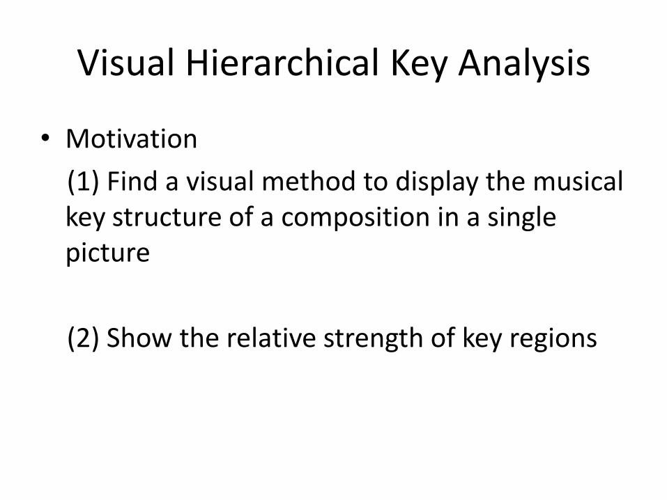
• Motivation

(1) Find a visual method to display the musical key structure of a composition in a single picture

(2) Show the relative strength of key regions

Computational Key Identification

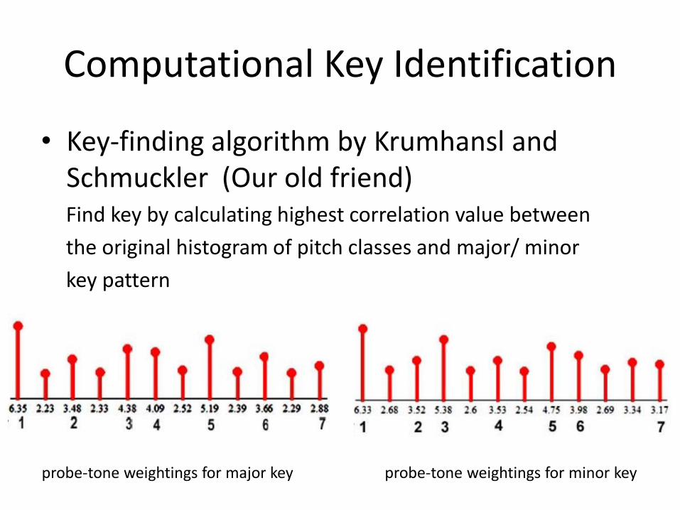
• Key-finding algorithm by Krumhansl and Schmuckler (Our old friend)Find key by calculating highest correlation value between

the original histogram of pitch classes and major/ minor

key pattern

probe-tone weightings for major key probe-tone weightings for minor key

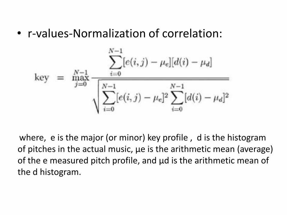
• r-values-Normalization of correlation:

where, e is the major (or minor) key profile , d is the histogram of pitches in the actual music, µe is the arithmetic mean (average) of the e measured pitch profile, and µd is the arithmetic mean of the d histogram.

Musical Key Modulation

• Too much music is analyzed at once, fewer important keys are suppressed

• Too little music is analyzed at once, the chordal structure of the music is analyzed, instead of the key structure

• What’s proper?

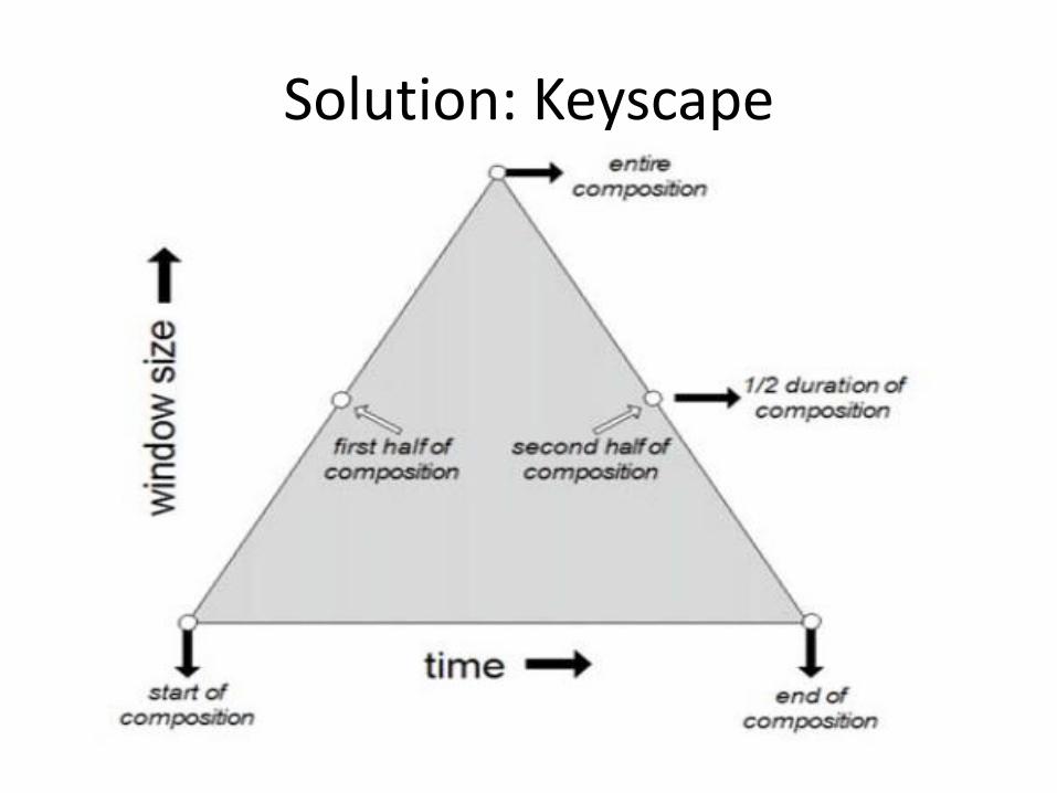
Solution: Keyscape

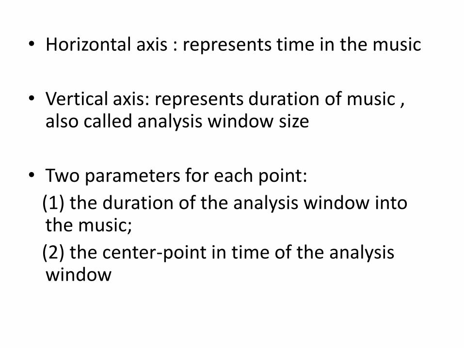
• Horizontal axis : represents time in the music

• Vertical axis: represents duration of music , also called analysis window size

• Two parameters for each point:

(1) the duration of the analysis window into the music;

(2) the center-point in time of the analysis window

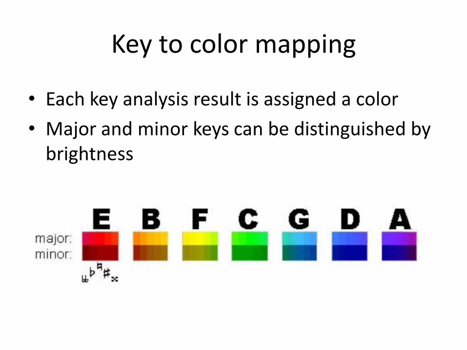
Key to color mapping

• Each key analysis result is assigned a color

• Major and minor keys can be distinguished by brightness

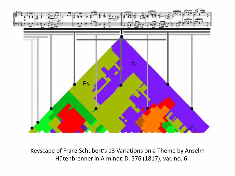
Keyscape of Franz Schubert’s 13 Variations on a Theme by Anselm Hütenbrenner in A minor, D. 576 (1817), var. no. 6.

A

F#

Keyscape VS landscape painting

• Bottom part: small-scale key features such as chords

- same as foreground in landscape painting

• Top part: large-scale key of the composition

- same as background in landscape painting

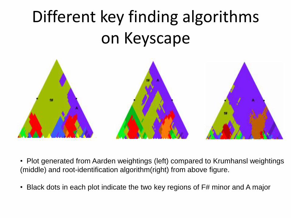
Different key finding algorithms on Keyscape

• Plot generated from Aarden weightings (left) compared to Krumhansl weightings

(middle) and root-identification algorithm(right) from above figure.

• Black dots in each plot indicate the two key regions of F# minor and A major

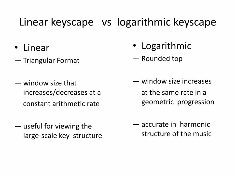
Linear keyscape vs logarithmic keyscape

• Linear — Triangular Format

— window size that increases/decreases at a

constant arithmetic rate

— useful for viewing the large-scale key structure

• Logarithmic— Rounded top

— window size increases

at the same rate in a geometric progression

— accurate in harmonic structure of the music

Linear keyscape vs logarithmic keyscape

• Both are applied to Divertimento no. 4, K 439b, mvmt. 1 composed by W.A. Mozart

C

G F

CG

Some examples of various styles of music

• Analysis of the Prelude from J.S. Bach's Cello Suite, BWV 1007(?)

Aarden weights used on the left and Krumhansl weights on the right

Some examples of various styles of music

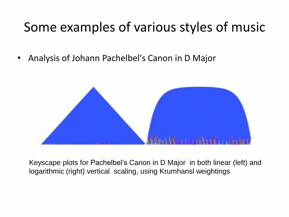
• Analysis of Johann Pachelbel's Canon in D Major

Keyscape plots for Pachelbel’s Canon in D Major in both linear (left) and

logarithmic (right) vertical scaling, using Krumhansl weightings

Some examples of various styles of music

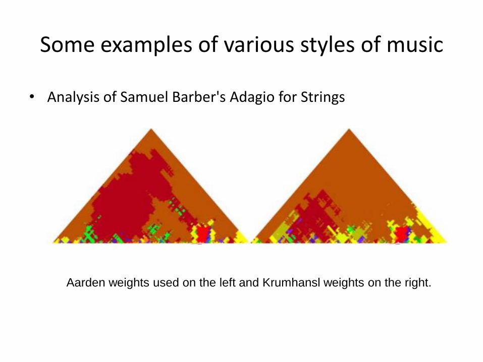
• Analysis of Samuel Barber's Adagio for Strings

Aarden weights used on the left and Krumhansl weights on the right.

Some examples of various styles of music

• Analysis of Anton Webern's Piano Variations, Op. 27, first movement (twelve-tone music, destroying tonal center)

Aarden weights used on the left and Krumhansl weights on the right.

Further Application of Scapes

• Scapes in Comparative Analysis of Multiple Music Performance

—Timescapes : corresponding to beat duration

—Dynascapes : corresponding to loudness

—Scape plots of parallel feature sequences

Procedure

• Choose one performance to be the reference for a particular plot

• For each cell in the scape plot, measure the correlation between the reference performance and all other performances, then make note of the performance which has the highest correlation value

• Color the cell with a unique hue assigned to that highest-correlating performance.

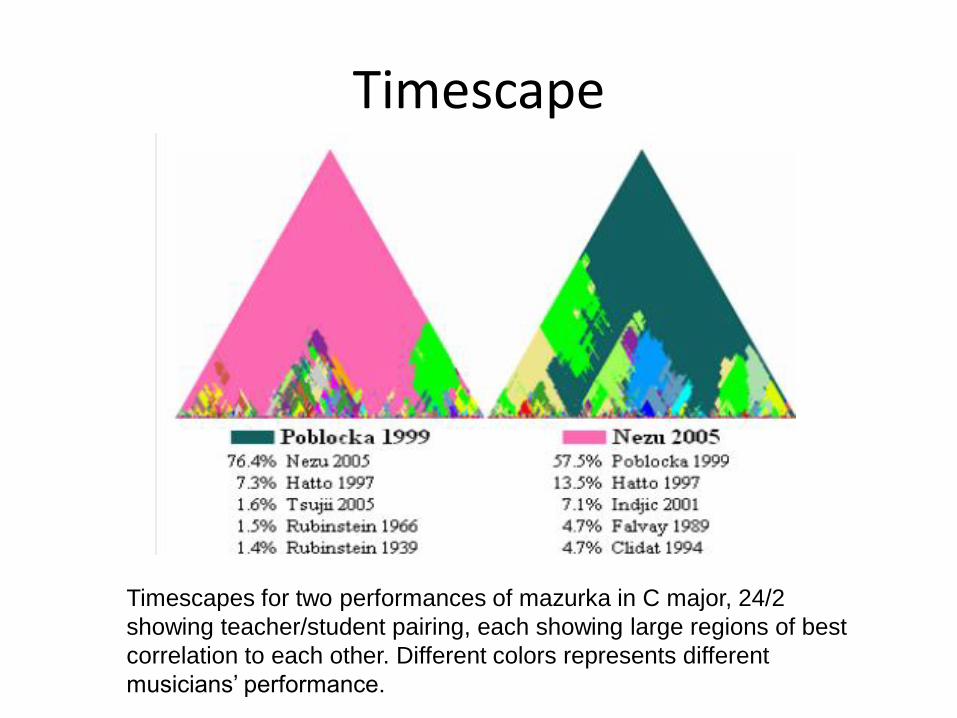
Timescape

Timescapes for two performances of mazurka in C major, 24/2

showing teacher/student pairing, each showing large regions of best

correlation to each other. Different colors represents different

musicians’ performance.

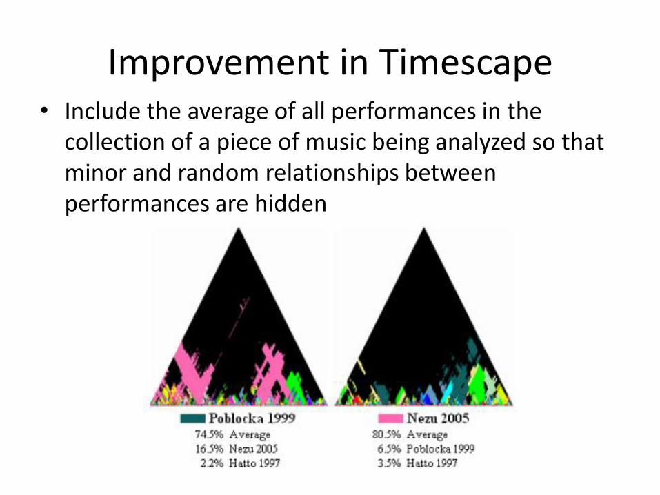
Improvement in Timescape• Include the average of all performances in the

collection of a piece of music being analyzed so that minor and random relationships between performances are hidden

Dynascapes

Two dynascapes of mazurka in C #minor, 63/2,showing

early/late career pairing of performers.

• Beat level amplitude measurements

• Less unique to a single individual performer-loudness defined in compositions

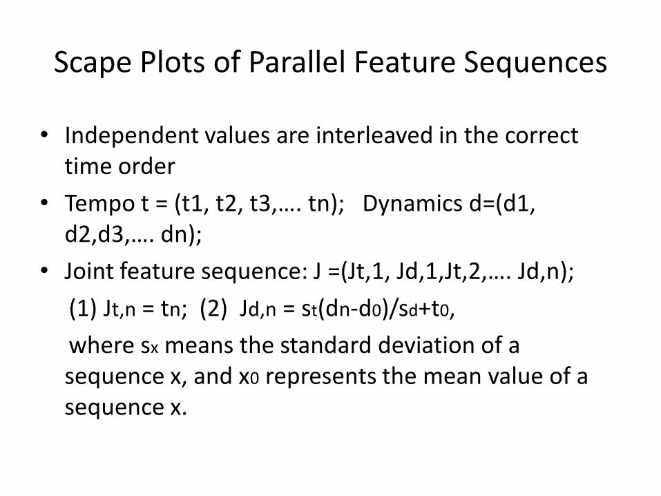
Scape Plots of Parallel Feature Sequences

• Independent values are interleaved in the correct time order

• Tempo t = (t1, t2, t3,…. tn); Dynamics d=(d1, d2,d3,…. dn);

• Joint feature sequence: J =(Jt,1, Jd,1,Jt,2,…. Jd,n);

(1) Jt,n = tn; (2) Jd,n = st(dn-d0)/sd+t0,

where sx means the standard deviation of a sequence x, and x0 represents the mean value of a sequence x.

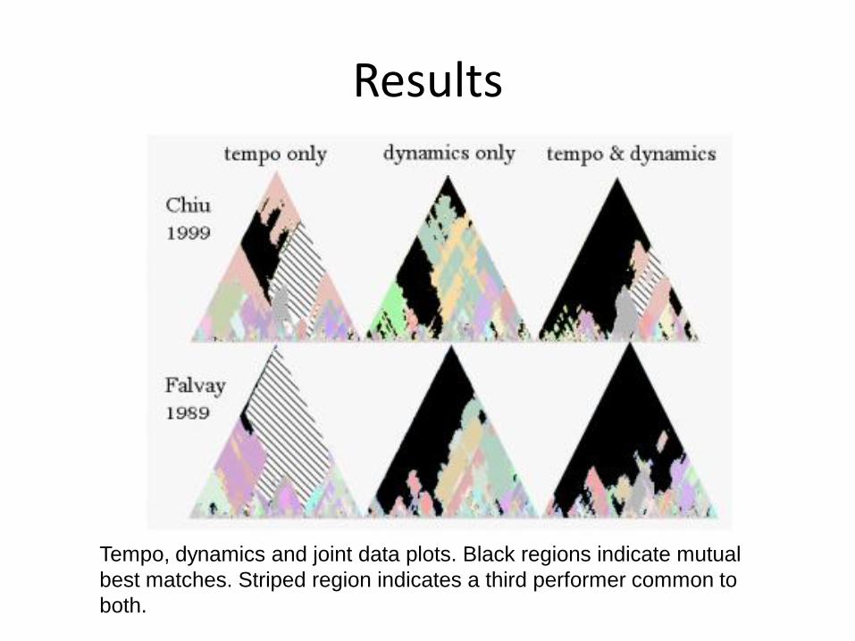
Results

Tempo, dynamics and joint data plots. Black regions indicate mutual

best matches. Striped region indicates a third performer common to

both.

Conclusion

• Keyscape provides a efficient and straightforward visual hierarchical key analysis.

• Scape plots are a step towards identifying important relations and can show where in a performance similarities are occurring.