Visual Exploration of Complex Functions

Elias Wegert

Abstract The technique of domain coloring allows one to represent complexfunctions as images on their domain. It endows functions with an individual faceand may serve as simple and efficient tool for their visual exploration. The empha-sis of this paper is on phase plots, a special variant of domain coloring. Thoughthese images utilize only the argument (phase) of a function and neglect its modulus,analytic (and meromorphic) functions are uniquely determined by their phase plotup to a positive constant factor. Following (Wegert in Not AMS 58:78–780, 2011[49], Wegert in Visual Complex Functions. An Introduction with Phase Portraits,Springer Basel, 2012 [53]), we introduce phase plots and several of their modifi-cations and explain how properties of functions can be reconstructed from theseimages. After a survey of related results, the main part is devoted to a number ofapplications which illustrate the usefulness of phase plots in teaching and research.

Keywords Complex functions · Visualization · Special functions · Analytic land-scape · Phase plot · Phase portrait · Argument principle · Padé approximation ·Riemann zeta function · Gravitational lenses · Filter designMathematics Subject Classification (2010). Primary 30-01; Secondary 30A99 ·33-01

1 Introduction

Graphical representations of functions belong to themost useful tools inmathematicsand its applications. While graphs of (scalar) real-valued functions can be depictedeasily, the situation is quite different for complex functions. Even the graph of a

E. Wegert (B)Institute of Applied Mathematics, TU Bergakademie Freiberg,Akademiestraße 6, 09596 Freiberg, Germanye-mail: wegert@math.tu-freiberg.de

© Springer International Publishing Switzerland 2016T. Qian and L.G. Rodino (eds.), Mathematical Analysis, Probabilityand Applications – Plenary Lectures, Springer Proceedingsin Mathematics & Statistics 177, DOI 10.1007/978-3-319-41945-9_10

253

254 E. Wegert

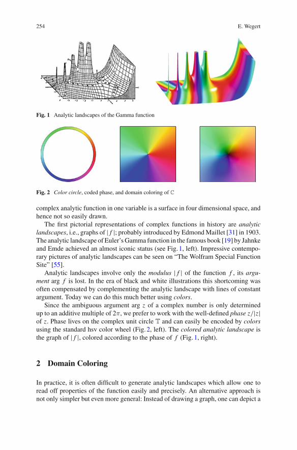
Fig. 1 Analytic landscapes of the Gamma function

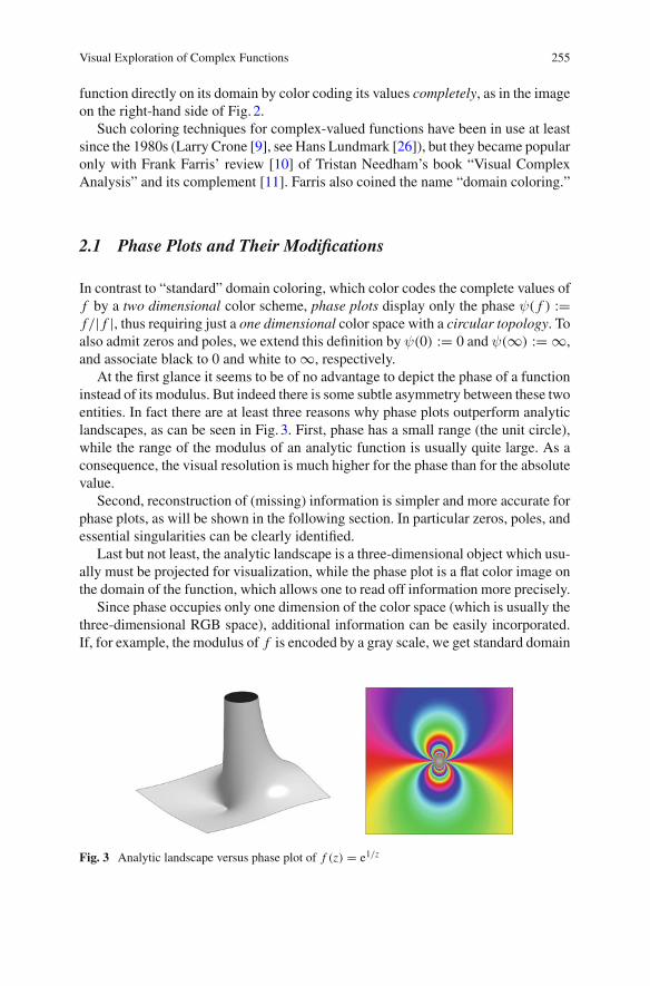
Fig. 2 Color circle, coded phase, and domain coloring of C

complex analytic function in one variable is a surface in four dimensional space, andhence not so easily drawn.

The first pictorial representations of complex functions in history are analyticlandscapes, i.e., graphs of | f |; probably introduced by EdmondMaillet [31] in 1903.The analytic landscape of Euler’sGamma function in the famous book [19] by Jahnkeand Emde achieved an almost iconic status (see Fig. 1, left). Impressive contempo-rary pictures of analytic landscapes can be seen on “The Wolfram Special FunctionSite” [55].

Analytic landscapes involve only the modulus | f | of the function f , its argu-ment arg f is lost. In the era of black and white illustrations this shortcoming wasoften compensated by complementing the analytic landscape with lines of constantargument. Today we can do this much better using colors.

Since the ambiguous argument arg z of a complex number is only determinedup to an additive multiple of 2π, we prefer to work with the well-defined phase z/|z|of z. Phase lives on the complex unit circle T and can easily be encoded by colorsusing the standard hsv color wheel (Fig. 2, left). The colored analytic landscape isthe graph of | f |, colored according to the phase of f (Fig. 1, right).

2 Domain Coloring

In practice, it is often difficult to generate analytic landscapes which allow one toread off properties of the function easily and precisely. An alternative approach isnot only simpler but even more general: Instead of drawing a graph, one can depict a

Visual Exploration of Complex Functions 255

function directly on its domain by color coding its values completely, as in the imageon the right-hand side of Fig. 2.

Such coloring techniques for complex-valued functions have been in use at leastsince the 1980s (Larry Crone [9], see Hans Lundmark [26]), but they became popularonly with Frank Farris’ review [10] of Tristan Needham’s book “Visual ComplexAnalysis” and its complement [11]. Farris also coined the name “domain coloring.”

2.1 Phase Plots and Their Modifications

In contrast to “standard” domain coloring, which color codes the complete values off by a two dimensional color scheme, phase plots display only the phase ψ( f ) :=f/| f |, thus requiring just a one dimensional color space with a circular topology. Toalso admit zeros and poles, we extend this definition by ψ(0) := 0 and ψ(∞) := ∞,and associate black to 0 and white to ∞, respectively.

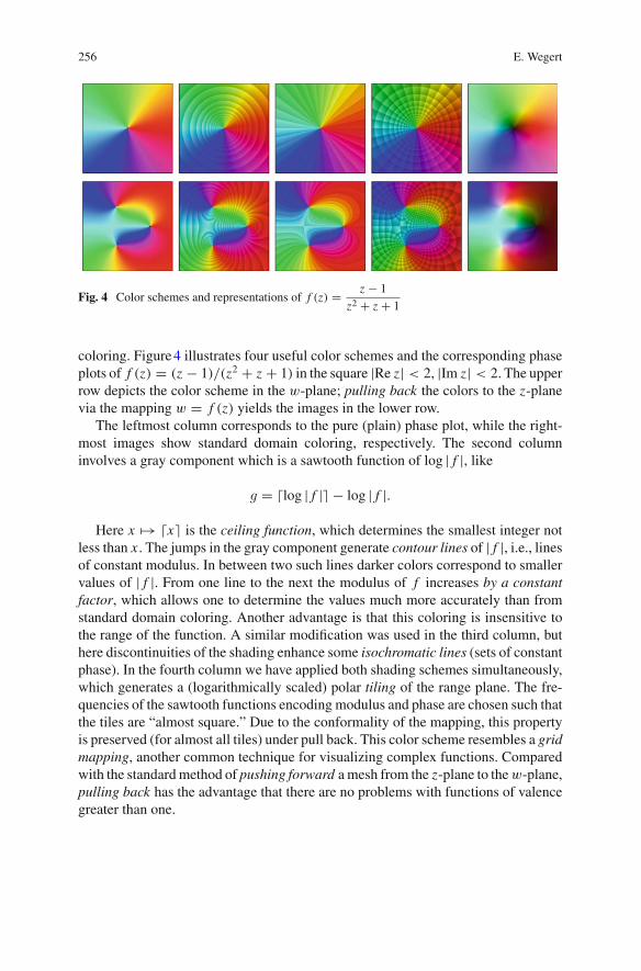
At the first glance it seems to be of no advantage to depict the phase of a functioninstead of its modulus. But indeed there is some subtle asymmetry between these twoentities. In fact there are at least three reasons why phase plots outperform analyticlandscapes, as can be seen in Fig. 3. First, phase has a small range (the unit circle),while the range of the modulus of an analytic function is usually quite large. As aconsequence, the visual resolution is much higher for the phase than for the absolutevalue.

Second, reconstruction of (missing) information is simpler and more accurate forphase plots, as will be shown in the following section. In particular zeros, poles, andessential singularities can be clearly identified.

Last but not least, the analytic landscape is a three-dimensional object which usu-ally must be projected for visualization, while the phase plot is a flat color image onthe domain of the function, which allows one to read off information more precisely.

Since phase occupies only one dimension of the color space (which is usually thethree-dimensional RGB space), additional information can be easily incorporated.If, for example, the modulus of f is encoded by a gray scale, we get standard domain

Fig. 3 Analytic landscape versus phase plot of f (z) = e1/z

256 E. Wegert

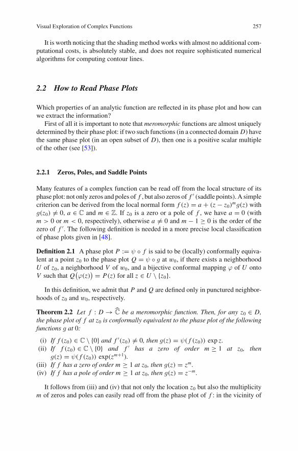
Fig. 4 Color schemes and representations of f (z) = z − 1

z2 + z + 1

coloring. Figure4 illustrates four useful color schemes and the corresponding phaseplots of f (z) = (z − 1)/(z2 + z + 1) in the square |Re z| < 2, |Im z| < 2. The upperrow depicts the color scheme in the w-plane; pulling back the colors to the z-planevia the mapping w = f (z) yields the images in the lower row.

The leftmost column corresponds to the pure (plain) phase plot, while the right-most images show standard domain coloring, respectively. The second columninvolves a gray component which is a sawtooth function of log | f |, like

g = �log | f |� − log | f |.

Here x �→ �x� is the ceiling function, which determines the smallest integer notless than x . The jumps in the gray component generate contour lines of | f |, i.e., linesof constant modulus. In between two such lines darker colors correspond to smallervalues of | f |. From one line to the next the modulus of f increases by a constantfactor, which allows one to determine the values much more accurately than fromstandard domain coloring. Another advantage is that this coloring is insensitive tothe range of the function. A similar modification was used in the third column, buthere discontinuities of the shading enhance some isochromatic lines (sets of constantphase). In the fourth column we have applied both shading schemes simultaneously,which generates a (logarithmically scaled) polar tiling of the range plane. The fre-quencies of the sawtooth functions encoding modulus and phase are chosen such thatthe tiles are “almost square.” Due to the conformality of the mapping, this propertyis preserved (for almost all tiles) under pull back. This color scheme resembles a gridmapping, another common technique for visualizing complex functions. Comparedwith the standardmethod of pushing forward amesh from the z-plane to thew-plane,pulling back has the advantage that there are no problems with functions of valencegreater than one.

Visual Exploration of Complex Functions 257

It is worth noticing that the shading method works with almost no additional com-putational costs, is absolutely stable, and does not require sophisticated numericalalgorithms for computing contour lines.

2.2 How to Read Phase Plots

Which properties of an analytic function are reflected in its phase plot and how canwe extract the information?

First of all it is important to note that meromorphic functions are almost uniquelydetermined by their phase plot: if two such functions (in a connected domain D) havethe same phase plot (in an open subset of D), then one is a positive scalar multipleof the other (see [53]).

2.2.1 Zeros, Poles, and Saddle Points

Many features of a complex function can be read off from the local structure of itsphase plot: not only zeros and poles of f , but also zeros of f ′ (saddle points). A simplecriterion can be derived from the local normal form f (z) = a + (z − z0)mg(z) withg(z0) �= 0, a ∈ C and m ∈ Z. If z0 is a zero or a pole of f , we have a = 0 (withm > 0 or m < 0, respectively), otherwise a �= 0 and m − 1 ≥ 0 is the order of thezero of f ′. The following definition is needed in a more precise local classificationof phase plots given in [48].

Definition 2.1 A phase plot P := ψ ◦ f is said to be (locally) conformally equiva-lent at a point z0 to the phase plot Q = ψ ◦ g at w0, if there exists a neighborhoodU of z0, a neighborhood V of w0, and a bijective conformal mapping ϕ of U ontoV such that Q

(ϕ(z)

) = P(z) for all z ∈ U \ {z0}.In this definition, we admit that P and Q are defined only in punctured neighbor-

hoods of z0 and w0, respectively.

Theorem 2.2 Let f : D → C be a meromorphic function. Then, for any z0 ∈ D,the phase plot of f at z0 is conformally equivalent to the phase plot of the followingfunctions g at 0:

(i) If f (z0) ∈ C \ {0} and f ′(z0) �= 0, then g(z) = ψ( f (z0)) exp z.(ii) If f (z0) ∈ C \ {0} and f ′ has a zero of order m ≥ 1 at z0, then

g(z) = ψ( f (z0)) exp(zm+1).(iii) If f has a zero of order m ≥ 1 at z0, then g(z) = zm.(iv) If f has a pole of order m ≥ 1 at z0, then g(z) = z−m.

It follows from (iii) and (iv) that not only the location z0 but also the multiplicitym of zeros and poles can easily read off from the phase plot of f : in the vicinity of

258 E. Wegert

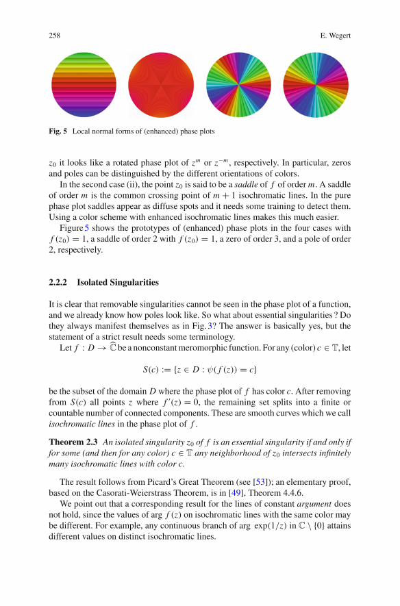
Fig. 5 Local normal forms of (enhanced) phase plots

z0 it looks like a rotated phase plot of zm or z−m , respectively. In particular, zerosand poles can be distinguished by the different orientations of colors.

In the second case (ii), the point z0 is said to be a saddle of f of order m. A saddleof order m is the common crossing point of m + 1 isochromatic lines. In the purephase plot saddles appear as diffuse spots and it needs some training to detect them.Using a color scheme with enhanced isochromatic lines makes this much easier.

Figure5 shows the prototypes of (enhanced) phase plots in the four cases withf (z0) = 1, a saddle of order 2 with f (z0) = 1, a zero of order 3, and a pole of order2, respectively.

2.2.2 Isolated Singularities

It is clear that removable singularities cannot be seen in the phase plot of a function,and we already know how poles look like. So what about essential singularities ? Dothey always manifest themselves as in Fig. 3? The answer is basically yes, but thestatement of a strict result needs some terminology.

Let f : D → C be a nonconstantmeromorphic function. For any (color) c ∈ T, let

S(c) := {z ∈ D : ψ( f (z)) = c}

be the subset of the domain D where the phase plot of f has color c. After removingfrom S(c) all points z where f ′(z) = 0, the remaining set splits into a finite orcountable number of connected components. These are smooth curves which we callisochromatic lines in the phase plot of f .

Theorem 2.3 An isolated singularity z0 of f is an essential singularity if and only iffor some (and then for any color) c ∈ T any neighborhood of z0 intersects infinitelymany isochromatic lines with color c.

The result follows from Picard’s Great Theorem (see [53]); an elementary proof,based on the Casorati-Weierstrass Theorem, is in [49], Theorem 4.4.6.

We point out that a corresponding result for the lines of constant argument doesnot hold, since the values of arg f (z) on isochromatic lines with the same color maybe different. For example, any continuous branch of arg exp(1/z) in C \ {0} attainsdifferent values on distinct isochromatic lines.

Visual Exploration of Complex Functions 259

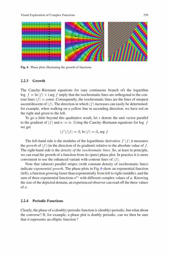
Fig. 6 Phase plots illustrating the growth of functions

2.2.3 Growth

The Cauchy–Riemann equations for (any continuous branch of) the logarithmlog f = ln | f | + i arg f imply that the isochromatic lines are orthogonal to the con-tour lines | f | = const. Consequently, the isochromatic lines are the lines of steepestascent/descent of | f |. The direction in which | f | increases can easily be determined:for example, when walking on a yellow line in ascending direction, we have red onthe right and green to the left.

To go a little beyond this qualitative result, let s denote the unit vector parallelto the gradient of | f | and n := is. Using the Cauchy–Riemann equations for log fwe get

| f ′|/| f | = ∂s ln | f | = ∂n arg f.

The left-hand side is the modulus of the logarithmic derivative f ′/ f ; it measuresthe growth of | f | (in the direction of its gradient) relative to the absolute value of f .The right-hand side is the density of the isochromatic lines. So, at least in principle,we can read the growth of a function from its (pure) phase plot. In practice it is moreconvenient to use the enhanced variant with contour lines of | f |.

Note that (almost) parallel stripes (with constant density of isochromatic lines)indicate exponential growth. The phase plots in Fig. 6 show an exponential function(left), a function growing faster than exponentially from left to right (middle), and thesum of three exponential functions eaz with different complex values of a. Knowingthe size of the depicted domain, an experienced observer can read off the three valuesof a.

2.2.4 Periodic Functions

Clearly, the phase of a (doubly) periodic function is (doubly) periodic, but what aboutthe converse? If, for example, a phase plot is doubly periodic, can we then be surethat it represents an elliptic function?

260 E. Wegert

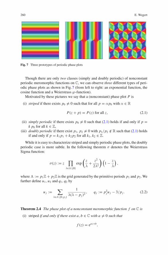
Fig. 7 Three prototypes of periodic phase plots

Though there are only two classes (simply and doubly periodic) of nonconstantperiodic meromorphic functions on C, we can observe three different types of peri-odic phase plots as shown in Fig. 7 (from left to right: an exponential function, thecosine function and a Weierstrass ℘-function).

Motivated by these pictures we say that a (nonconstant) phase plot P is

(i) striped if there exists p0 �= 0 such that for all p = αp0 with α ∈ R

P(z + p) = P(z) for all z, (2.1)

(ii) simply periodic if there exists p0 �= 0 such that (2.1) holds if and only if p =k p0 for all k ∈ Z,

(iii) doubly periodic if there exist p1, p2 �= 0 with p1/p2 /∈ R such that (2.1) holdsif and only if p = k1 p1 + k2 p2 for all k1, k2 ∈ Z.

While it is easy to characterize striped and simply periodic phase plots, the doublyperiodic case is more subtle. In the following theorem σ denotes the WeierstrassSigma function:

σ(z) := z∏

λ∈�\{0}exp

(z

λ+ z2

2λ2

)(1 − z

λ

),

where� := p1Z + p2Z is the grid generated by the primitive periods p1 and p2. Wefurther define u1, u2 and q1, q2 by

u j :=∑

λ∈�\{0,p j }

1

λ(λ − p j )2, q j := p2

j u j − 3/p j . (2.2)

Theorem 2.4 The phase plot of a nonconstant meromorphic function f on C is

(i) striped if and only if there exist a, b ∈ C with a �= 0 such that

f (z) = eaz+b,

Visual Exploration of Complex Functions 261

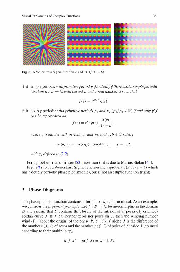
Fig. 8 A Weierstrass Sigma function σ and σ(z)/σ(z − b)

(ii) simplyperiodicwith primitive period p if and only if there exist a simply periodicfunction g : C → C with period p and a real number a such that

f (z) = eaz/p g(z),

(iii) doubly periodic with primitive periods p1 and p2 (p1/p2 /∈ R) if and only if fcan be represented as

f (z) = eaz g(z)σ(z)

σ(z − b),

where g is elliptic with periods p1 and p2, and a, b ∈ C satisfy

Im (ap j ) ≡ Im (bq j ) (mod 2π), j = 1, 2,

with q j defined in (2.2).

For a proof of (i) and (ii) see [53], assertion (iii) is due to Marius Stefan [40].Figure8 shows aWeierstrass Sigma function and a quotient σ(z)/σ(z − b)which

has a doubly periodic phase plot (middle), but is not an elliptic function (right).

3 Phase Diagrams

The phase plot of a function contains information which is nonlocal. As an example,we consider the argument principle: Let f : D → C be meromorphic in the domainD and assume that D contains the closure of the interior of a (positively oriented)Jordan curve J . If f has neither zeros nor poles on J , then the winding numberwindJ Pf (about the origin) of the phase Pf := ψ ◦ f along J is the difference ofthe number n( f, J ) of zeros and the number p( f, J ) of poles of f inside J (countedaccording to their multiplicity),

n( f, J ) − p( f, J ) = windJ Pf .

262 E. Wegert

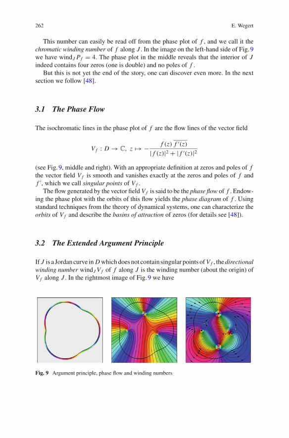
This number can easily be read off from the phase plot of f , and we call it thechromatic winding number of f along J . In the image on the left-hand side of Fig. 9we have windJ Pf = 4. The phase plot in the middle reveals that the interior of Jindeed contains four zeros (one is double) and no poles of f .

But this is not yet the end of the story, one can discover even more. In the nextsection we follow [48].

3.1 The Phase Flow

The isochromatic lines in the phase plot of f are the flow lines of the vector field

V f : D → C, z �→ − f (z) f ′(z)| f (z)|2 + | f ′(z)|2

(see Fig. 9, middle and right). With an appropriate definition at zeros and poles of fthe vector field V f is smooth and vanishes exactly at the zeros and poles of f andf ′, which we call singular points of V f .The flow generated by the vector field V f is said to be the phase flow of f . Endow-

ing the phase plot with the orbits of this flow yields the phase diagram of f . Usingstandard techniques from the theory of dynamical systems, one can characterize theorbits of V f and describe the basins of attraction of zeros (for details see [48]).

3.2 The Extended Argument Principle

If J is a Jordan curve in D whichdoes not contain singular points ofV f , thedirectionalwinding number windJ V f of f along J is the winding number (about the origin) ofV f along J . In the rightmost image of Fig. 9 we have

Fig. 9 Argument principle, phase flow and winding numbers

Visual Exploration of Complex Functions 263

windJ Pf = 1, windJ V f = 2.

Analyzing the phase diagram using index theory reveals a relation between the twowinding numbers of f along J and the numbers n( f ′, J ) and p( f ′, J ) of zeros andpoles of f ′ inside J , respectively.

Theorem 3.1 ([48]) Let f be meromorphic in D and assume that the positivelyoriented Jordan curve J and its interior are contained in D. If neither f nor f ′ havezeros or poles on J , then

n( f ′, J ) − p( f ′, J ) = windJ Pf − windJ V f

Note that (at least in principle, but not always in practice) both winding numberscan be read off from the phase plot of f in an arbitrarily small neighborhood of J .

If f is holomorphic, the argument principle and Theorem 3.1 allow one to deter-mine the number of zeros of f and f ′ inside J from the phase plot of f near J .In Fig. 9 (left) we have windJ Pf = 4 and windJ V f = 1, so that n( f, J ) = 4 andn( f ′, J ) = 3.

An important special case pertains to the situation when f is holomorphic andthe isochromatic lines of f are nowhere tangent to J . Since the latter implieswindJ V f =1, Theorem 3.1 tells us that then n( f ′, J ) = n( f, J ) − 1. This yieldsa short proof of Walsh’s theorem on the location of critical points of Blaschke prod-ucts [46–48].

4 Applications

In this section we discuss applications of phase plots which we believe to be useful—though in some examples the mathematical background is rather trivial.

4.1 Software Implementation

When one needs to compute special functions numerically, it is tempting to downloadcode which is freely available on the internet. In many cases this may be an easy andefficient way to solve the problem, but one should be aware that there is no guaranteethat software does what it claims to do.

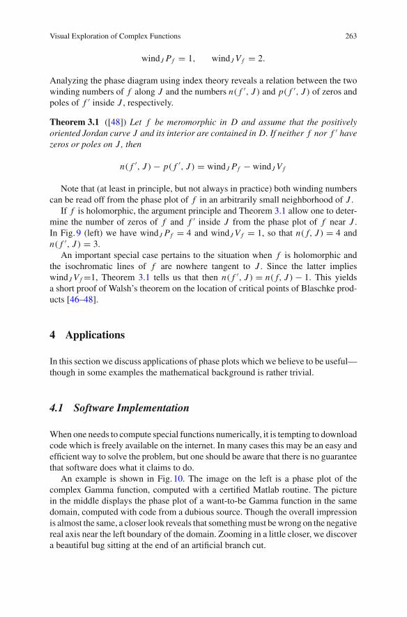
An example is shown in Fig. 10. The image on the left is a phase plot of thecomplex Gamma function, computed with a certified Matlab routine. The picturein the middle displays the phase plot of a want-to-be Gamma function in the samedomain, computed with code from a dubious source. Though the overall impressionis almost the same, a closer look reveals that somethingmust bewrong on the negativereal axis near the left boundary of the domain. Zooming in a little closer, we discovera beautiful bug sitting at the end of an artificial branch cut.

264 E. Wegert

Fig. 10 A bug in software for evaluating the Gamma function

Fig. 11 Implementations of the logarithmic Gamma Function

Since this is not the only incidentwhich can be reported, one should be very carefulwhen using software without knowing what it really computes. Though looking atphase plots can by no means ensure correctness of computations, it may help todiscover some inconsistencies quite easily.

4.2 Multivalued Functions

Computations involvingmultivalued functions, like complexnth roots or the complexlogarithm, are often challenging because usually only their main branch is imple-mented in standard software. In particular, composing such functions without takingcare for choosing the appropriate branches may lead to fallacious results.

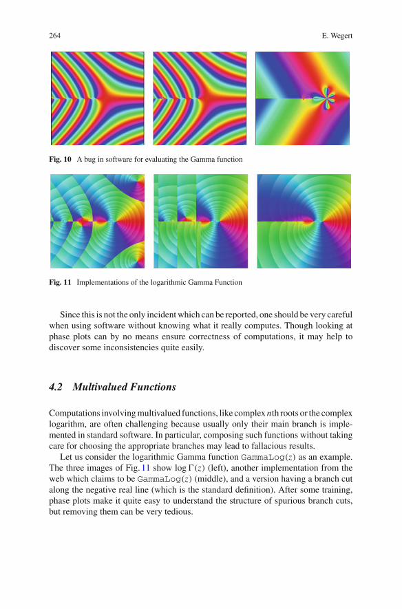
Let us consider the logarithmic Gamma function GammaLog(z) as an example.The three images of Fig. 11 show log�(z) (left), another implementation from theweb which claims to be GammaLog(z) (middle), and a version having a branch cutalong the negative real line (which is the standard definition). After some training,phase plots make it quite easy to understand the structure of spurious branch cuts,but removing them can be very tedious.

Visual Exploration of Complex Functions 265

4.3 Riemann Surfaces

Phase plots may serve as convenient tool for constructing Riemann surfaces. Wedemonstrate this for the Riemann surface of the inverse of the sine function f (z) =sin z. Basically this procedure involves three steps:Step 1. Look at the phase plot of f in the z-plane and determine the basins ofattraction of the zeros (first row of Fig. 12). In the case at hand the basins are verticalstripes kπ < Re z < (k + 1)π, k ∈ Z. Every such basin is mapped onto a copy ofthe complex w-plane, slit along the rays [−∞,−1] and [1,+∞] (second row).Step 2. Change the coloring of the z-plane to the standard color scheme (phase plotof the identity, see first row of Fig. 13).Step 3. Push the colors forward from the fundamental domains to the w-plane byw = f (z). This generates phase plots of f −1 on the different sheets of its Riemannsurface (second row of Fig. 13).

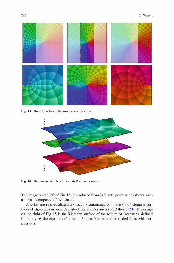
Gluing the rims of branch cuts according to their neighboring relations (whichusually, but not always, can be seen from the phase plots), yields the Riemann surfaceon which the phase plot of g can be displayed (see Fig. 14).

Thomas Banchoff [5] and Michael Trott [43, 44] described techniques for visual-izing complex functions ondomain-coloredRiemann surfaces. This topicwas studiedin more detail by Konrad Poehlke and Konstantin Polthier [33]. In two subsequentpapers [34] and [32] (with M.Niesen) they propose algorithms for the automaticconstruction of Riemann surfaces with prescribed branch points and branch indices.

Fig. 12 The sine function mapping strips to C

266 E. Wegert

Fig. 13 Three branches of the inverse sine function

Fig. 14 The inverse sine function on its Riemann surface

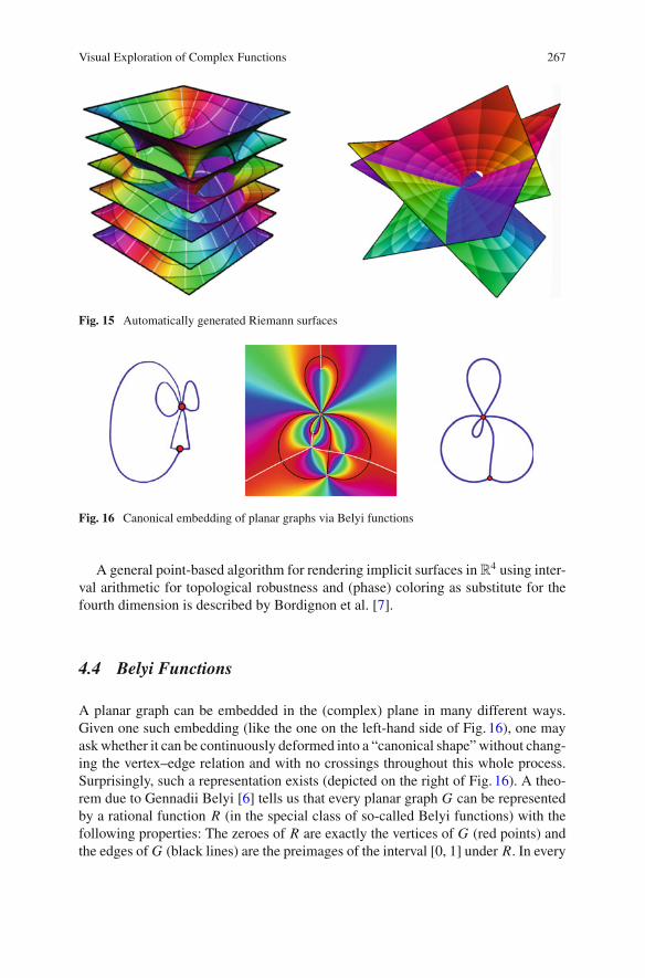
The image on the left of Fig. 15 (reproduced from [32] with permission) shows sucha surface composed of five sheets.

Another (more specialized) approach to automated computation of Riemann sur-faces of algebraic curves is described in Stefan Kranich’s PhD thesis [24]. The imageon the right of Fig. 15 is the Riemann surface of the folium of Descartes, definedimplicitly by the equation z3 + w3 − 3zw = 0 (reprinted in scaled form with per-mission).

Visual Exploration of Complex Functions 267

Fig. 15 Automatically generated Riemann surfaces

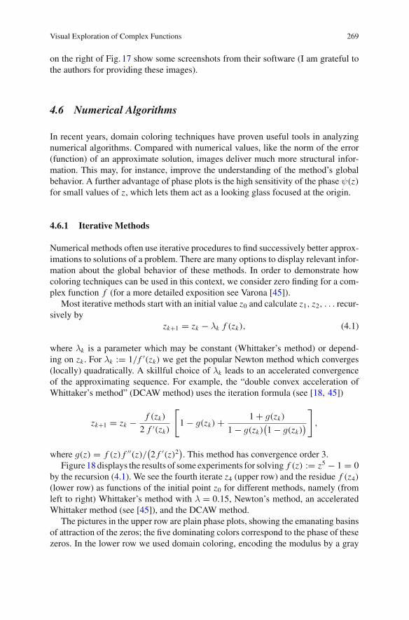
Fig. 16 Canonical embedding of planar graphs via Belyi functions

A general point-based algorithm for rendering implicit surfaces inR4 using inter-val arithmetic for topological robustness and (phase) coloring as substitute for thefourth dimension is described by Bordignon et al. [7].

4.4 Belyi Functions

A planar graph can be embedded in the (complex) plane in many different ways.Given one such embedding (like the one on the left-hand side of Fig. 16), one mayaskwhether it can be continuously deformed into a “canonical shape”without chang-ing the vertex–edge relation and with no crossings throughout this whole process.Surprisingly, such a representation exists (depicted on the right of Fig. 16). A theo-rem due to Gennadii Belyi [6] tells us that every planar graph G can be representedby a rational function R (in the special class of so-called Belyi functions) with thefollowing properties: The zeroes of R are exactly the vertices of G (red points) andthe edges of G (black lines) are the preimages of the interval [0, 1] under R. In every

268 E. Wegert

face of G there is exactly one pole of R (white points) and the preimages of [1,+∞](white lines) connect the poles to one point (gray) on each of the edges bounding theface containing that pole. (The area outside the graph is considered to be a face withits pole at infinity.) Moreover, all edges run into a vertex with equal angles betweenneighboring edges and the (white) lines originating at the poles intersect the edgesperpendicularly. Last but not least, every face is the basin of attraction (see Sect. 3and [48]) of the associated pole (with respect to the reverse phase flow).

The actual computation of the Belyi function associated with a given graph is achallenging problem. Donald Marshall developed an approach via conformal weld-ing [27, 28] and implemented it using his software Zipper [29, 30]. I am grateful tohim for providing the coefficients of the Belyi function shown in Fig. 16.

4.5 Filters and Controllers

In signal and control theory (linear, causal, time invariant, and stable) systems aredescribed by transfer functions, which are analytic in the right half plane. In practice,most transfer functions are rational functions with poles in the left half plane. In thefrequency domain the system acts on an input as multiplication operator with itstransfer function T . In particular, the frequency response T (iω) tells one what thesystem does with harmonic input signals eiωt : The values |T (iω)| and arg T (iω) arethe gain and the phase shift induced by the system operating at frequency ω.

The phase plot on the left of Fig. 17 is the transfer function of a Butterworthfilter—a low pass filter, which damps high frequency signals. This can be seen fromits frequency response on the imaginary axis: the white segment is the passbandwhere |T (iω)| ≈ 1, in the stopband (black) |T (iω)| decays for increasing values ofω. Using the contour lines and the phase coloring one can read off the frequencyresponse directly from the phase plot of T and, for instance, construct Bode andNyquist plots.

Santiago Garrido and Luis Moreno [15] developed more elaborate techniquesinvolving phase plots for designing controllers. The two images in the middle and

Fig. 17 Design of filters and controllers

Visual Exploration of Complex Functions 269

on the right of Fig. 17 show some screenshots from their software (I am grateful tothe authors for providing these images).

4.6 Numerical Algorithms

In recent years, domain coloring techniques have proven useful tools in analyzingnumerical algorithms. Compared with numerical values, like the norm of the error(function) of an approximate solution, images deliver much more structural infor-mation. This may, for instance, improve the understanding of the method’s globalbehavior. A further advantage of phase plots is the high sensitivity of the phase ψ(z)for small values of z, which lets them act as a looking glass focused at the origin.

4.6.1 Iterative Methods

Numerical methods often use iterative procedures to find successively better approx-imations to solutions of a problem. There are many options to display relevant infor-mation about the global behavior of these methods. In order to demonstrate howcoloring techniques can be used in this context, we consider zero finding for a com-plex function f (for a more detailed exposition see Varona [45]).

Most iterative methods start with an initial value z0 and calculate z1, z2, . . . recur-sively by

zk+1 = zk − λk f (zk), (4.1)

where λk is a parameter which may be constant (Whittaker’s method) or depend-ing on zk . For λk := 1/ f ′(zk) we get the popular Newton method which converges(locally) quadratically. A skillful choice of λk leads to an accelerated convergenceof the approximating sequence. For example, the “double convex acceleration ofWhittaker’s method” (DCAW method) uses the iteration formula (see [18, 45])

zk+1 = zk − f (zk)

2 f ′(zk)

[

1 − g(zk) + 1 + g(zk)

1 − g(zk)(1 − g(zk)

)

]

,

where g(z) = f (z) f ′′(z)/(2 f ′(z)2

). This method has convergence order 3.

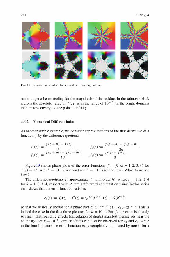
Figure18 displays the results of some experiments for solving f (z) := z5 − 1 = 0by the recursion (4.1). We see the fourth iterate z4 (upper row) and the residue f (z4)(lower row) as functions of the initial point z0 for different methods, namely (fromleft to right) Whittaker’s method with λ = 0.15, Newton’s method, an acceleratedWhittaker method (see [45]), and the DCAW method.

The pictures in the upper row are plain phase plots, showing the emanating basinsof attraction of the zeros; the five dominating colors correspond to the phase of thesezeros. In the lower row we used domain coloring, encoding the modulus by a gray

270 E. Wegert

Fig. 18 Iterates and residues for several zero-finding methods

scale, to get a better feeling for the magnitude of the residue. In the (almost) blackregions the absolute value of f (z4) is in the range of 10−15, in the bright domainsthe iterates converge to the point at infinity.

4.6.2 Numerical Differentiation

As another simple example, we consider approximations of the first derivative of afunction f by the difference quotients

f1(z) := f (z + h) − f (z)

h, f2(z) := f (z + h) − f (z − h)

2h,

f3(z) := f (z + ih) − f (z − ih)

2ih, f4(z) := f2(z) + f3(z)

2.

Figure19 shows phase plots of the error functions f ′ − fk (k = 1, 2, 3, 4) forf (z) = 1/z with h = 10−3 (first row) and h = 10−5 (second row). What do we seehere?

The difference quotients fk approximate f ′ with order hn , where n = 1, 2, 2, 4for k = 1, 2, 3, 4, respectively. A straightforward computation using Taylor seriesthen shows that the error function satisfies

ek(z) := fk(z) − f ′(z) = ck hn f (n+1)(z) + O(hn+1)

so that we basically should see a phase plot of ck f (n+1)(z) = ck(−z)−n−2. This isindeed the case in the first three pictures for h = 10−3. For f4 the error is alreadyso small, that rounding effects (cancelation of digits) manifest themselves near theboundary. For h = 10−5, similar effects can also be observed for e2 and e3, whilein the fourth picture the error function e4 is completely dominated by noise (for a

Visual Exploration of Complex Functions 271

Fig. 19 Error functions for numerical differentiation

Fig. 20 Evaluation of Cauchy integrals

computer expert the emerging structure may reveal information about the imple-mented arithmetic).

The most interesting observation is that one can read off the approximation ordern directly: applying the method to f (z) = z−1, the resulting phase plot shows a poleof order n + 2 at the origin. Similar types of experiments can be designed for otherapproximation methods.

4.6.3 Numerical Integration

Evaluation of integrals is another topic which can nicely be illustrated and studiedusing phase plots. In Fig. 20, we demonstrate this for a Cauchy integral of an analyticfunction f . The exact values of the integral are displayed in the figure on the left-handside. Outside the contour of integration the integral vanishes, at points z surroundedby the contour its values are equal to k f (z), where k is the winding number of thecontour about z (here k is either 1 or 2).

272 E. Wegert

The other two figures show approximations of the integral, evaluated by the trape-zoidal rule with 200 and 1200 nodes, respectively.We see poles, sitting at the contourof integration, induced by the pole of the Cauchy kernel. The gear-like pattern in theexterior domain has almost parallel isochromatic lines, indicating rapid decay of thefunction (in the direction perpendicular to the contour); it is bounded by a chain ofzeros aligned along the contour of integration. This chainmay be related to Jentzsch’stheorem and its generalizations ([8, 20, 46]).

Austin, Kravanja and Trefethen [1] used phase plots in order to compare differentmethods (Cauchy integrals, polynomial and rational interpolation) for computing val-ues f (z) and f (m)(z) of analytic and meromorphic functions in a disk from samplesat the boundary of that disk.

4.6.4 Padé Approximation

Phase plots of rational functions can “visually approximate” any image, drawn solelywith saturated colors from the hsv color wheel (for a precise statement see [50]).Particularly nice images arise from rational functions with zeros and poles formingspecial patterns, as it happens, for instance, in Padé approximation. In turn, theseimages may help to understand special aspects of these approximations.

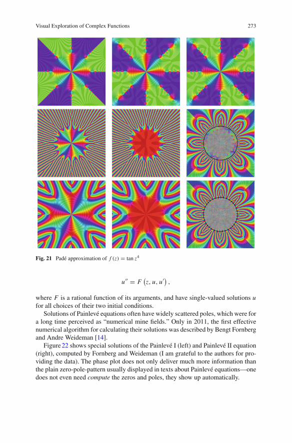
The first row of Fig. 21 shows the function f (z) = tan z4 to be approximated(left), and two Padé approximants of order [100, 100]. The function depicted in themiddle is computed by a standard method, the function on the right is the outputof a stabilized (“robust”) algorithm developed by Gonnet et al. [17]. Though thepictures can barely be distinguished, the structural differences become obvious inthe next two rows, depicting phase plots of the numerator polynomial p (left) andthe denominator polynomial q (middle), as well as the error function f − f[100,100](right). The upper row corresponds to the standard algorithm, while the lower rowvisualizes the output of the stabilized algorithm. Apparently the first one producesa lot of spurious zeros in both polynomials p and q, which are (almost) canceled inthe quotient p/q.

The black line in the error plots on the right-hand side is the unit circle. Thealmost(!) unstructured part in the middle (the influence of the zero-pole-cancelationis seen here) is due to small fluctuations about zero.

The computations are performed with the Matlab routine padeapprox of theChebfun toolbox (for details see [17]).

4.6.5 Differential Equations

Numerous classes of special functions (Bessel, Airy, hypergeometric, etc.) arise assolutions of second order ordinary differential equations (ODEs). Computing thesefunctions often requires elaborate numerical methods. A particularly hard case isgiven by the six Painlevé equations, which are prototypes of equations

Visual Exploration of Complex Functions 273

Fig. 21 Padé approximation of f (z) = tan z4

u′′ = F(z, u, u′) ,

where F is a rational function of its arguments, and have single-valued solutions ufor all choices of their two initial conditions.

Solutions of Painlevé equations often have widely scattered poles, which were fora long time perceived as “numerical mine fields.” Only in 2011, the first effectivenumerical algorithm for calculating their solutions was described by Bengt Fornbergand Andre Weideman [14].

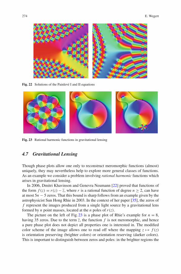
Figure22 shows special solutions of the Painlevé I (left) and Painlevé II equation(right), computed by Fornberg and Weideman (I am grateful to the authors for pro-viding the data). The phase plot does not only deliver much more information thanthe plain zero-pole-pattern usually displayed in texts about Painlevé equations—onedoes not even need compute the zeros and poles, they show up automatically.

274 E. Wegert

Fig. 22 Solutions of the Painlevé I and II equations

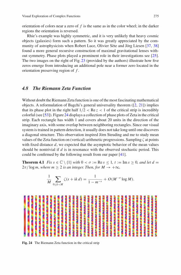
Fig. 23 Rational harmonic functions in gravitational lensing

4.7 Gravitational Lensing

Though phase plots allow one only to reconstruct meromorphic functions (almost)uniquely, they may nevertheless help to explore more general classes of functions.As an example we consider a problem involving rational harmonic functions whicharises in gravitational lensing.

In 2006, Dmitri Khavinson and Genevra Neumann [22] proved that functions ofthe form f (z) = r(z) − z, where r is a rational function of degree n ≥ 2, can haveat most 5n − 5 zeros. That this bound is sharp follows from an example given by theastrophysicist Sun Hong Rhie in 2003. In the context of her paper [35], the zeros off represent the images produced from a single light source by a gravitational lensformed by n point masses, located at the n poles of r(z).

The picture on the left of Fig. 23 is a phase plot of Rhie’s example for n = 8,having 35 zeros. Due to the term z, the function f is not meromorphic, and hencea pure phase plot does not depict all properties one is interested in. The modifiedcolor scheme of the image allows one to read off where the mapping z �→ f (z)is orientation preserving (brighter colors) or orientation reserving (darker colors).This is important to distinguish between zeros and poles: in the brighter regions the

Visual Exploration of Complex Functions 275

orientation of colors near a zero of f is the same as in the color wheel; in the darkerregions the orientation is reversed.

Rhie’s example was highly symmetric, and it is very unlikely that heavy cosmicobjects (galaxies) form such a pattern. So it was greatly appreciated by the com-munity of astrophysicists when Robert Luce, Olivier Sète and Jörg Liesen [37, 38]found a more general recursive construction of maximal gravitational lenses with-out symmetry. Phase plots played a prominent role in their investigations see [25].The two images on the right of Fig. 23 (provided by the authors) illustrate how fivezeros emerge from introducing an additional pole near a former zero located in theorientation preserving region of f .

4.8 The Riemann Zeta Function

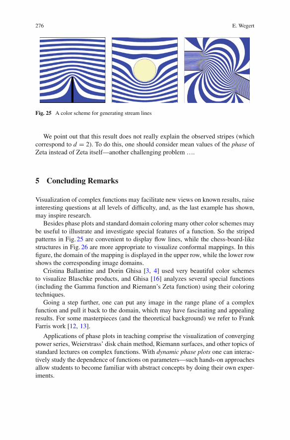
Without doubt theRiemannZeta function is one of themost fascinatingmathematicalobjects. A reformulation of Bagchi’s general universality theorem ([2, 21]) impliesthat its phase plot in the right half 1/2 < Re z < 1 of the critical strip is incrediblycolorful (see [53]). Figure24 displays a collection of phase plots of Zeta in the criticalstrip. Each rectangle has width 1 and covers about 20 units in the direction of theimaginary axis, with some overlap between neighboring rectangles. Since our visualsystem is trained in pattern detection, it usually does not take long until one discoversa diagonal structure. This observation inspired Jörn Steuding and me to study meanvalues of the Zeta function on (vertical) arithmetic progressions. Sampling ζ at pointswith fixed distance d, we expected that the asymptotic behavior of the mean valuesshould be nontrivial if d is in resonance with the observed stochastic period. Thiscould be confirmed by the following result from our paper [41].

Theorem 4.1 Fix s ∈ C \ {1} with 0 < σ := Re s ≤ 1, t := Im s ≥ 0, and let d =2π/ logm, where m ≥ 2 is an integer. Then, for M → +∞,

1

M

∑

0≤k<M

ζ(s + ik d) = 1

1 − m−s+ O(M−σ log M).

Fig. 24 The Riemann Zeta function in the critical strip

276 E. Wegert

Fig. 25 A color scheme for generating stream lines

We point out that this result does not really explain the observed stripes (whichcorrespond to d = 2). To do this, one should consider mean values of the phase ofZeta instead of Zeta itself—another challenging problem ….

5 Concluding Remarks

Visualization of complex functions may facilitate new views on known results, raiseinteresting questions at all levels of difficulty, and, as the last example has shown,may inspire research.

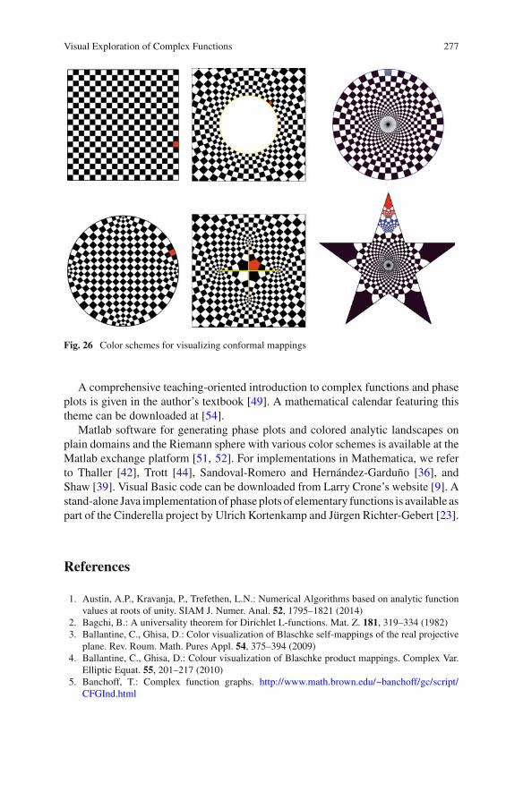
Besides phase plots and standard domain coloring many other color schemes maybe useful to illustrate and investigate special features of a function. So the stripedpatterns in Fig. 25 are convenient to display flow lines, while the chess-board-likestructures in Fig. 26 are more appropriate to visualize conformal mappings. In thisfigure, the domain of the mapping is displayed in the upper row, while the lower rowshows the corresponding image domains.

Cristina Ballantine and Dorin Ghisa [3, 4] used very beautiful color schemesto visualize Blaschke products, and Ghisa [16] analyzes several special functions(including the Gamma function and Riemann’s Zeta function) using their coloringtechniques.

Going a step further, one can put any image in the range plane of a complexfunction and pull it back to the domain, which may have fascinating and appealingresults. For some masterpieces (and the theoretical background) we refer to FrankFarris work [12, 13].

Applications of phase plots in teaching comprise the visualization of convergingpower series, Weierstrass’ disk chain method, Riemann surfaces, and other topics ofstandard lectures on complex functions. With dynamic phase plots one can interac-tively study the dependence of functions on parameters—such hands-on approachesallow students to become familiar with abstract concepts by doing their own exper-iments.

Visual Exploration of Complex Functions 277

Fig. 26 Color schemes for visualizing conformal mappings

A comprehensive teaching-oriented introduction to complex functions and phaseplots is given in the author’s textbook [49]. A mathematical calendar featuring thistheme can be downloaded at [54].

Matlab software for generating phase plots and colored analytic landscapes onplain domains and the Riemann sphere with various color schemes is available at theMatlab exchange platform [51, 52]. For implementations in Mathematica, we referto Thaller [42], Trott [44], Sandoval-Romero and Hernández-Garduño [36], andShaw [39]. Visual Basic code can be downloaded from Larry Crone’s website [9]. Astand-alone Java implementationof phase plots of elementary functions is available aspart of the Cinderella project by Ulrich Kortenkamp and Jürgen Richter-Gebert [23].

References

1. Austin, A.P., Kravanja, P., Trefethen, L.N.: Numerical Algorithms based on analytic functionvalues at roots of unity. SIAM J. Numer. Anal. 52, 1795–1821 (2014)

2. Bagchi, B.: A universality theorem for Dirichlet L-functions. Mat. Z. 181, 319–334 (1982)3. Ballantine, C., Ghisa, D.: Color visualization of Blaschke self-mappings of the real projective

plane. Rev. Roum. Math. Pures Appl. 54, 375–394 (2009)4. Ballantine, C., Ghisa, D.: Colour visualization of Blaschke product mappings. Complex Var.

Elliptic Equat. 55, 201–217 (2010)5. Banchoff, T.: Complex function graphs. http://www.math.brown.edu/~banchoff/gc/script/

CFGInd.html

278 E. Wegert

6. Belyi, G.V.: Galois extensions of a maximal cyclotomic field. Izvestiya Akademii Nauk SSSR14, 269–276 (1979). (Russian). English translation: Mathematics USSR Izvestija, 14, 247–256(1980)

7. Bordignon, A.L., Sa, L., Lopes, H., Pesco, S., de Figueiredo, L.H.: Point-based rendering ofimplicit surfaces in R4. Comput. Graph. 37, 873–884 (2013)

8. Blatt, H.P., Blatt, S., Luh, W.: On a generalization of Jentzsch’s theorem. J. Approx. Theory159, 26–38 (2009)

9. Crone, L.: Color graphs of complex functions. http://www1.math.american.edu/People/lcrone/ComplexPlot.html Accessed 17 Mar 2016

10. Farris, F.A.: Review of Visual Complex Analysis. By Tristan Needham. Am. Math. Monthly105, 570–576 (1998)

11. Farris, F.A.: Visualizing complex-valued functions in the plane. http://www.maa.org/visualizing-complex-valued-functions-in-the-plane (2016). Accessed 17 Mar 2016

12. Farris, F.A.: Symmetric yet organic: Fourier series as an artist’s tool. J. Math. Arts 7, 64–82(2013)

13. Farris, F.A.: Creating Symmetry: The Artful Mathematics of Wallpaper Patterns, 230p. Prince-ton University Press (2015)

14. Fornberg, B., Weideman, J.A.C.: A Numerical methodology for the Painlevé equations. J.Comput. Phys. 230, 5957–5973 (2011)

15. Garrido, S., Moreno, L.: PM diagram of the transfer function and its use in the design ofcontrollers. J. Math. Syst. Sci. 5, 138–149 (2015)

16. Ghisa, D.: Fundamental Domains and the Riemann Hypothesis, 148p. Lap Lambert AcademicPublishing (2012)

17. Gonnet, P., Güttel, S., Trefethen, L.N.: Robust Padé approximation via SVD. Siam Rev. 55,101–117 (2013)

18. Hernández, M.A.: An acceleration procedure of the Whittaker method by means of convexity.Zb. Rad. Prirod.-Mat. Fak. 20, 27–38 (1990)

19. Jahnke, E., Emde, F.: Funktionentafeln mit Formeln und Kurven. Teubner (1933)20. Jentzsch, R.: Untersuchungen zur Theorie der Folgen analytischer Funktionen. Acta. Math. 41,

219–251 (1918)21. Karatsuba, A.A., Voronin, S.M.: The Riemann Zeta-Function. Walter de Gruyter (1992)22. Khavinson, D., Neumann, G.: From the fundamental theorem of algebra to astrophysics: a

“harmonious” path. Not. AMS 55, 666–675 (2008)23. Kortenkamp, U., Richter-Gebert, J.: Phase Diagrams of Complex Functions. http://science-to-

touch.com/CJS/CindyJS/complexFunctions/ (2016). Accessed 17 Mar 201624. Kranich, S.: Continuity in dynamic geometry. An algorithmic approach. Ph.D. thesis, TU

Munich (2016)25. Luce, R., Sète, O., Liesen, J.: A note on the maximum number of zeros of r(z) − z. Comput.

Methods Funct. Theory 15, 439–448 (2015)26. Lundmark, H.: Visualizing complex analytic functions using domain coloring. http://users.mai.

liu.se/hanlu09/complex/domain_coloring.html (2016). Accessed 18 Mar 201627. Marshall, D.E.: Conformal welding for finitely connected regions. Comput. Methods Funct.

Theory 11, 655–669 (2011)28. Marshall, D.E.: Conformal welding and planar graphs. http://www.birs.ca/events/2015/5-day-

workshops/15w5052/videos/watch/201501120953-Marshall.html (2016). Accessed 15 Mar2016

29. Marshall, D.E.: Numerical conformal mapping software: zipper. https://www.math.washington.edu/~marshall/zipper.html (2016). Accessed 15 Mar 2016

30. Marshall, D.E., Rohde, S.: Convergence of a variant of the Zipper algorithm for conformalmapping. SIAM J. Numer. Anal. 45, 2577–2609 (2007)

31. Maillet, E.: Sur les lignes de décroissance maxima des modules et les équations algébraiquesou transcendantes. J. de l’Éc. Pol. 8, 75–95 (1903)

32. Nieser, M., Poelke, K., Polthier, K.: Automatic generation of Riemann surface meshes. In:Advances in Geometric Modeling and Processing. Lecture Notes in Computer Science, vol.6130, pp. 161–178. Springer (2010)

Visual Exploration of Complex Functions 279

33. Poelke, K., Polthier, K.: Lifted domain coloring. Comput. Graph. Forum 28, 735–742 (2009)34. Poelke, K., Polthier, K.: Domain coloring of complex functions: an implementation-oriented

introduction. IEEE Comput. Graphics Appl. 32, 90–97 (2012)35. Rhie, S.H.: n-point gravitational lenses with 5(n-1) images. ArXiv Astrophysics

arXiv:astro-ph/0305166 (2003)36. Sandoval-Romero, Á., Hernández-Garduño, A.: Domain coloring on the riemann sphere.Math.

J. 17 (2015)37. Sète, O., Luce, R., Liesen, J.: Perturbing rational harmonic functions by poles. Comput. Meth-

ods Funct. Theory 15, 9–35 (2015)38. Sète, O., Luce, R., Liesen, J.: Creating images by adding masses to gravitational point lenses.

Gen. Relativ. Gravit. 47, 42 (2015)39. Shaw, W.T.: Complex Analysis with Mathematica. Cambridge University Press (2006)40. Stefan, M.B.: On doubly periodic phases. Proc. Am. Math. Soc. 142, 3149–3152 (2011)41. Steuding, J., Wegert, E.: The Riemann zeta function on arithmetic progressions. Exp. Math.

21, 235–240 (2012)42. Thaller, B.: Visualization of complex functions. Math. J. 7, 163–180 (1999)43. Trott, M.: Visualization of Riemann surfaces of algebraic functions. Math. Educ. Res. 6, 15–36

(1997)44. Trott, M.: Visualization of Riemann surfaces. http://library.wolfram.com/infocenter/Demos/

15/ (2016). Accessed 17 Mar 201645. Varona, J.L.: Graphic and numerical comparison between iterative methods. Math. Intell. 24,

37–46 (2002)46. Walsh, J.L.: The location of critical points of analytic and harmonic functions. American

Mathematical Society Colloquium Publications 34, 386p, New York (1950)47. Walsh, J.L.: Note on the location of zeros of extremal polynomials in the non-Euclidean plane.

Acad. Serbe Sci. Publ. Inst. Math. 4, 157–160 (1952)48. Wegert, E.: Phase diagrams of meromorphic functions. Comput. Methods Funct. Theory 10,

639–661 (2010)49. Wegert, E.: Visual Complex Functions. An Introduction with Phase Portraits. Springer Basel

(2012)50. Wegert, E.: Complex functions and images. Computational Methods and Function Theory 13,

3–10 (2013)51. Wegert, E.: Phase plots of complex functions. http://www.mathworks.com/matlabcentral/

fileexchange/44375 (2016). Accessed 15 Mar 201652. Wegert, E.: The complex function explorer. http://www.mathworks.com/matlabcentral/

fileexchange/45464 (2016). Accessed 15 Mar 201653. Wegert, E., Semmler, G.: Phase plots of complex functions: a journey in illustration. Not. AMS

58, 768–780 (2011)54. Wegert, E., Semmler, G., Gorkin, P., Daepp, U.: Complex Beauties. Mathematical calendars

featuring phase plots. http://www.mathcalendar.net (2016). Accessed 15 Mar 201655. Wolfram Research, The Wolfram Functions Site. http://www.functions.wolfram.com (2016).

Accessed 15 Mar 2016