Vision Review:Image Processing

Course web page:www.cis.udel.edu/~cer/arv

September 17, 2002

Announcements

• Homework and paper presentation guidelines are up on web page

• Readings for next Tuesday: Chapters 6, 11.1, and 18

• For next Thursday: “Stochastic Road Shape Estimation”

Computer Vision Review Outline

• Image formation• Image processing• Motion & Estimation • Classification

Outline

• Images• Binary operators• Filtering

– Smoothing– Edge, corner detection

• Modeling, matching • Scale space

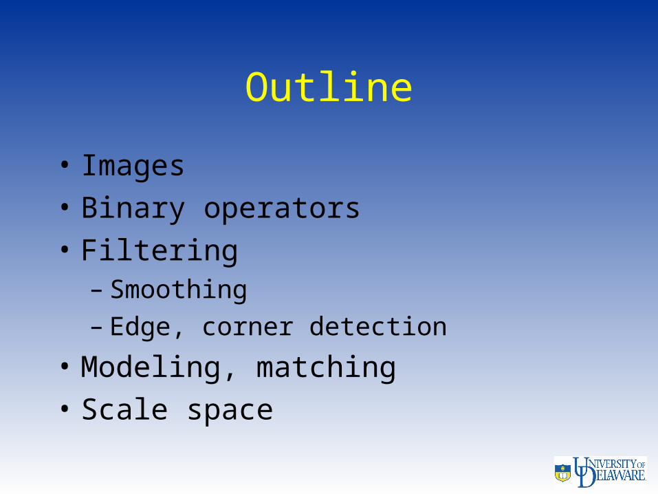
Images

• An image is a matrix of pixels Note: Matlab uses

• Resolution– Digital cameras: 1600 X 1200 at a

minimum– Video cameras: ~640 X 480

• Grayscale: generally 8 bits per pixel Intensities in range [0…255]

• RGB color: 3 8-bit color planes

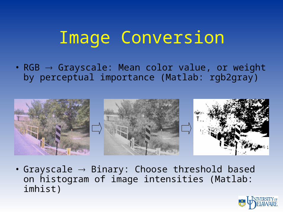
Image Conversion

• RGB Grayscale: Mean color value, or weight by perceptual importance (Matlab: rgb2gray)

• Grayscale Binary: Choose threshold based on histogram of image intensities (Matlab: imhist)

Color Representation

• RGB, HSV (hue, saturation, value), YUV, etc.

• Luminance: Perceived intensity• Chrominance: Perceived color

– HS(V), (Y)UV, etc.– Normalized RGB removes some

illumination dependence:

Binary Operations

• Dilation, erosion (Matlab: imdilate, imerode)– Dilation: All 0’s next to a 1 1 (Enlarge foreground)– Erosion: All 1’s next to a 0 0 (Enlarge background)

• Connected components– Uniquely label each n-connected region in binary image– 4- and 8-connectedness– Matlab: bwfill, bwselect

• Moments: Region statistics– Zeroth-order: Size– First-order: Position (centroid)– Second-order: Orientation

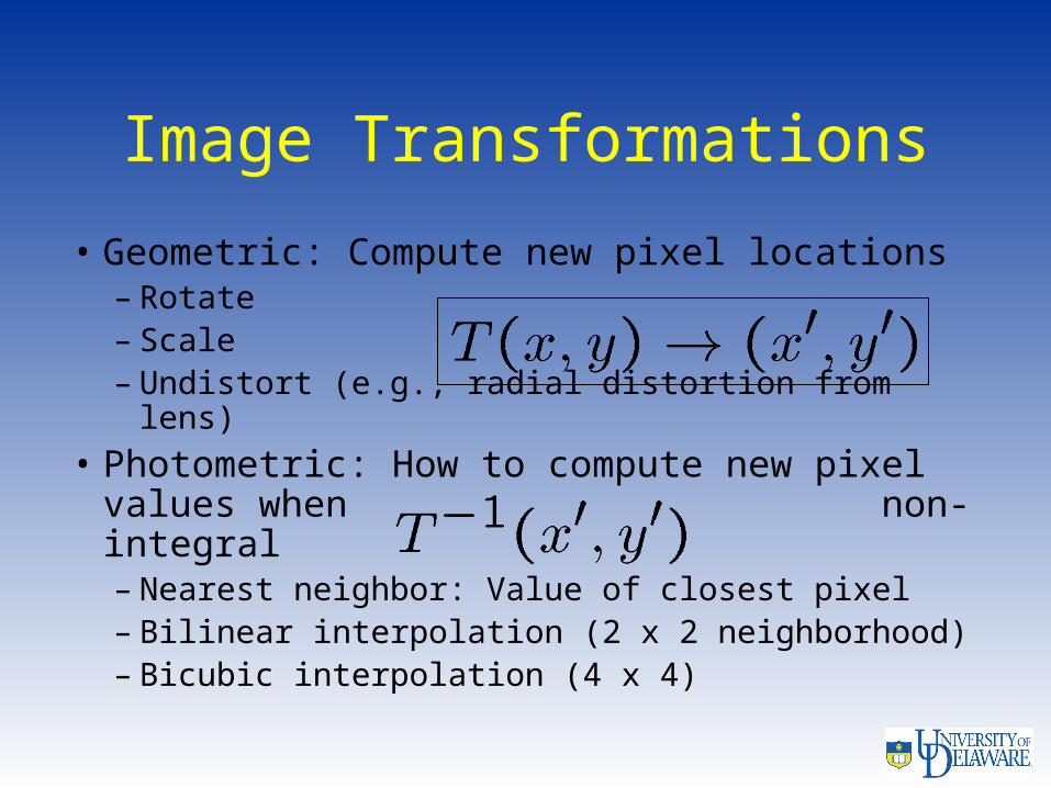
Image Transformations

• Geometric: Compute new pixel locations – Rotate– Scale– Undistort (e.g., radial distortion from lens)

• Photometric: How to compute new pixel values when non-integral– Nearest neighbor: Value of closest pixel– Bilinear interpolation (2 x 2 neighborhood)– Bicubic interpolation (4 x 4)

Bilinear Interpolation

• Idea: Blend four pixel values surrounding source, weighted by nearness

Vertical blend Horizontal blend

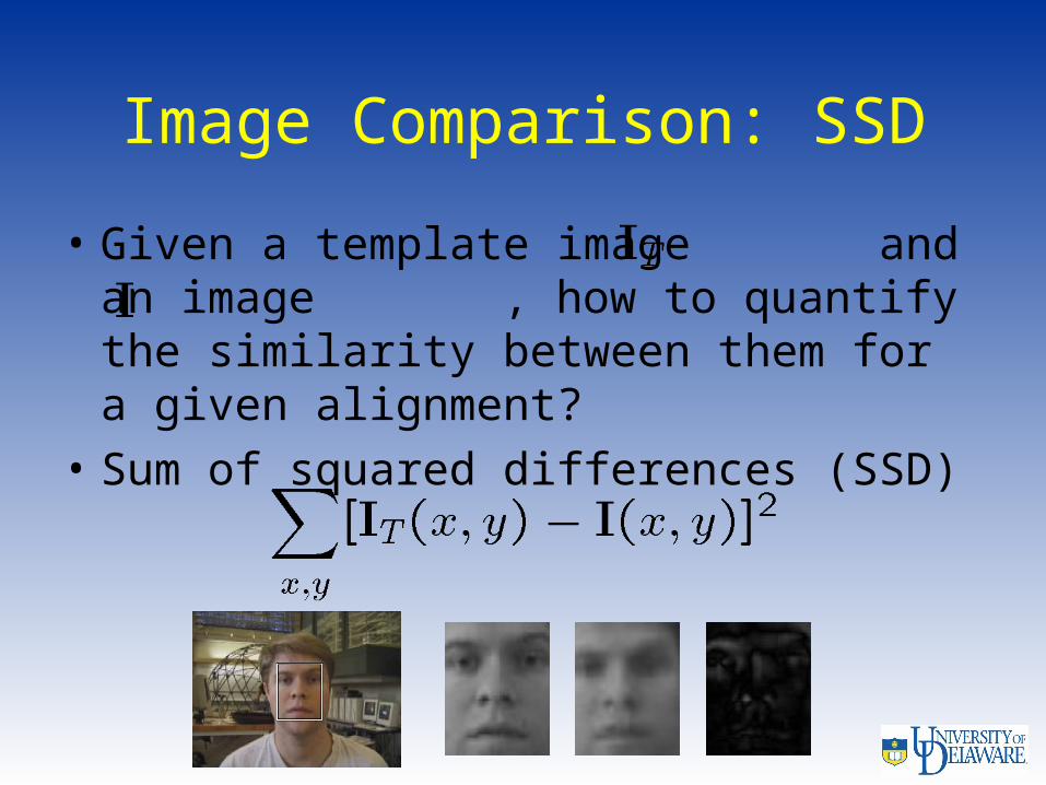
Image Comparison: SSD

• Given a template image and an image , how to quantify the similarity between them for a given alignment?

• Sum of squared differences (SSD)

Cross-Correlation for Template Matching

• Note that SSD formula can be written:

• First two terms fixed last term measures mismatch—the cross-correlation:

• In practice, normalize by image magnitude when shifting template to search for matches

Filtering

• Idea: Analyze neighborhood around some point in image with filter function ; put result in new image at corresponding location

• System properties– Shift invariance: Same inputs give same outputs,

regardless of location– Superposition: Output on sum of images = – Sum of outputs on separate images– Scaling: Output on scaled image = Scaled output on

image

• Linear shift invariance Convolution

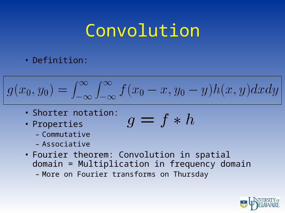
Convolution

• Definition:

• Shorter notation: • Properties

– Commutative– Associative

• Fourier theorem: Convolution in spatial domain = Multiplication in frequency domain– More on Fourier transforms on Thursday

Discrete Filtering

• Linear filter: Weighted sum of pixels over rectangular neighborhood—kernel defines weights

• Think of kernel as template being matched by correlation (Matlab: imfilter, filter2)

• Convolution: Correlation with kernel rotated 180– Matlab: conv2

• Dealing with image edges– Zero-padding– Border replication

111-121-1-11

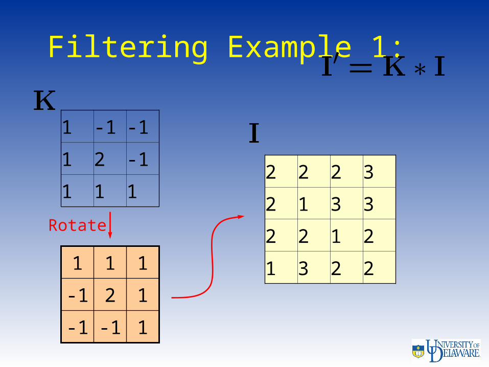
Filtering Example 1:

1 -1 -1

1 2 -1

1 1 12 2 2 3

2 1 3 3

2 2 1 2

1 3 2 2

Rotate

1-1-1

12-1

111

Step 1

3

2

1

2

2

1

3

2

32

21

22

32 5

3

2

1

2

2

1

3

2

32

21

22

32

1-2-1

24-1

111

1-1-1

12-1

111

Step 2

3

2

1

2

2

1

3

2

32

21

22

32 45

3

2

1

2

2

1

3

2

32

21

22

32

3-1-2

24-2

111

1-1-1

12-1

111

Step 3

3

2

1

2

2

1

3

2

32

21

22

32 4 45

3

2

1

2

2

1

3

2

32

21

22

32

3-3-1

34-2

111

1-1-1

12-1

111

Step 4

3

2

1

2

2

1

3

2

32

21

22

32 4 4 -25

3

2

1

2

2

1

3

2

32

21

22

32

1-3-3

16-2

111

1-1-1

12-1

111

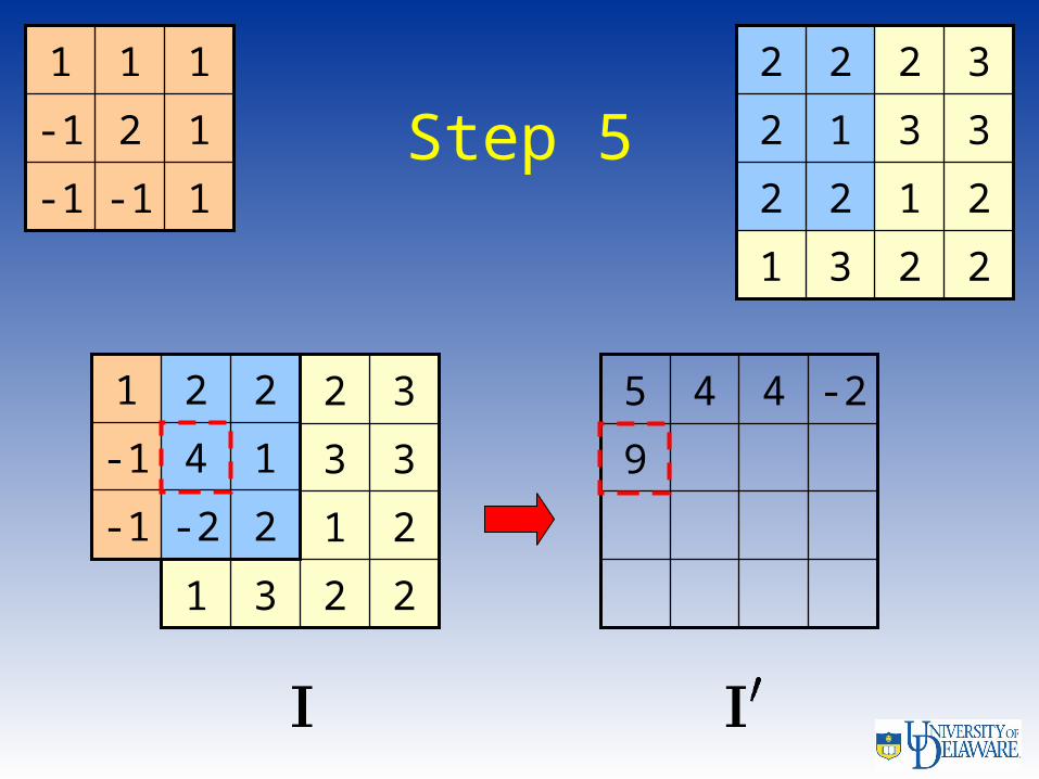
Step 5

3

2

1

2

2

1

3

2

32

21

22

32 4 4

9

-25

3

2

1

2

2

1

3

2

32

21

22

32

2-2-1

14-1

221

1-1-1

12-1

111

Step 6

3

2

1

2

2

1

3

2

32

21

22

32

6

4 4

9

-25

3

2

1

2

2

1

3

2

32

21

22

32

1-2-2

32-2

222

1-1-1

12-1

111

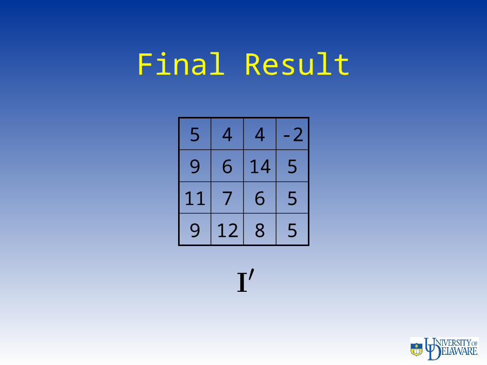
Final Result

12

7

6

4

8

6

14

4

59

59

511

-25

Separability

• Definition: 2-D kernel can be written as convolution of two 1-D kernels

• Advantage: Efficiency—Convolving image with kernel requires

multiplies vs. for non-separable kernel

Smoothing (Low-Pass) Filters

• Replace each pixel with average of neighbors

• Benefits: Suppress noise, aliasing• Disadvantage: Sharp features

blurred• Types

– Mean filter (box)– Median (nonlinear)– Gaussian

111

111

111

3 x 3 box filter

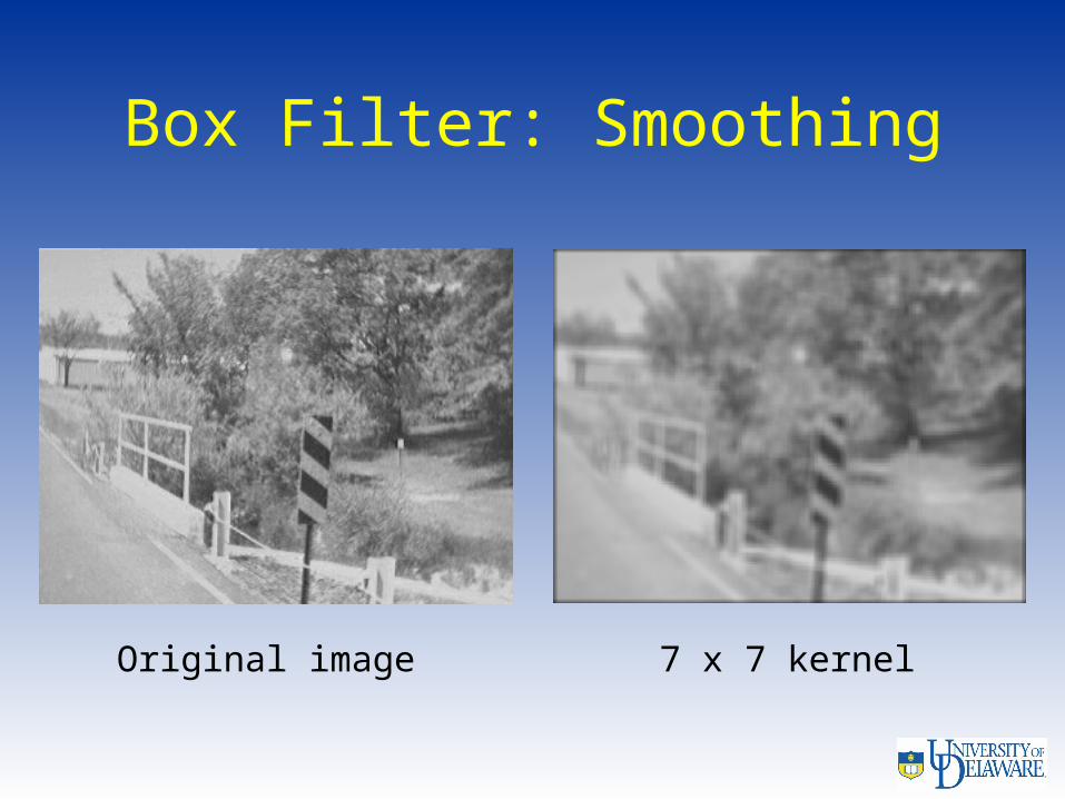
Box Filter: Smoothing

7 x 7 kernelOriginal image

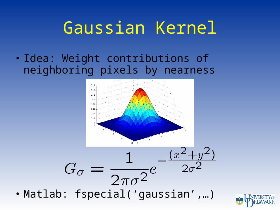
Gaussian Kernel

• Idea: Weight contributions of neighboring pixels by nearness

• Matlab: fspecial(‘gaussian’,…)

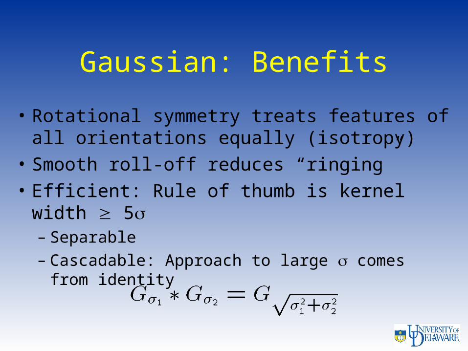
Gaussian: Benefits

• Rotational symmetry treats features of all orientations equally (isotropy)

• Smooth roll-off reduces “ringing”• Efficient: Rule of thumb is kernel width

5 – Separable– Cascadable: Approach to large comes

from identity

Gaussian: Smoothing

= 1 = 3

7 x 7kernel

Originalimage

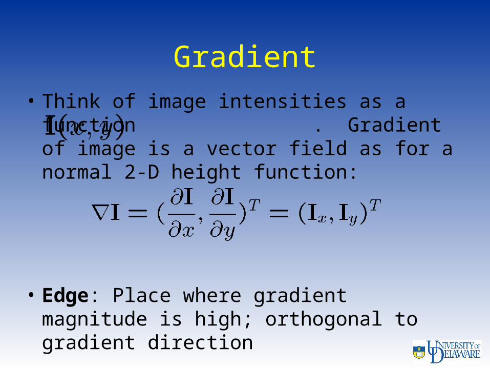
Gradient• Think of image intensities as a function

. Gradient of image is a vector field as for a normal 2-D height function:

• Edge: Place where gradient magnitude is high; orthogonal to gradient direction

Edge Causes

• Depth discontinuity• Surface orientation discontinuity• Reflectance discontinuity (i.e.,

change in surface material properties)

• Illumination discontinuity (e.g., shadow)

Edge Detection

• Edge Types– Step edge (ramp)– Line edge (roof)

• Searching for Edges:– Filter: Smooth image– Enhance: Apply numerical derivative

approximation– Detect: Threshold to find strong edges– Localize/analyze: Reject spurious edges,

include weak but justified edges

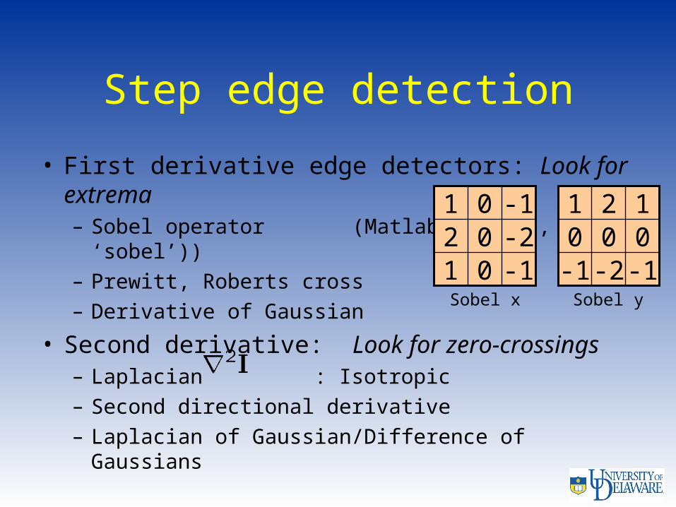
Step edge detection

• First derivative edge detectors: Look for extrema– Sobel operator

(Matlab: edge(I, ‘sobel’))– Prewitt, Roberts cross– Derivative of Gaussian

• Second derivative: Look for zero-crossings– Laplacian : Isotropic– Second directional derivative– Laplacian of Gaussian/Difference of Gaussians

-1-2-1000121

-101-202-101

Sobel x Sobel y

Derivative of Gaussian

Laplacian of Gaussian

• Matlab: fspecial(‘log’,…)

Edge Filtering Example

1 0 -1

2 0 -2

1 0 -10 0 2 2

0 0 2 2

0 0 2 2

0 0 2 2

Rotate

10-1

20-2

10-1

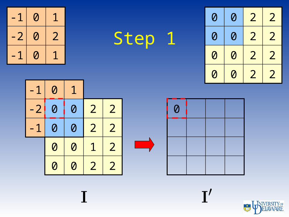
Step 1

0

0

1

2

2

1

2

2

22

20

20

22 0

0

0

0

0

2

2

2

2

20

20

20

20

00-1

00-2

10-1

10-1

20-2

10-1

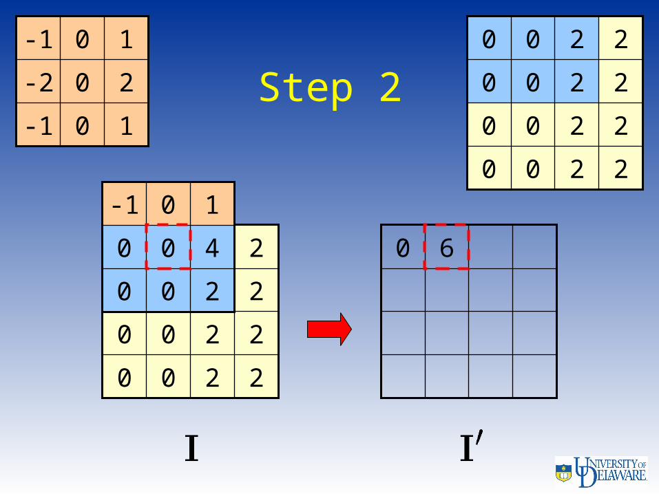
Step 2

0

0

1

2

2

2

3

2

22

20

20

22 60

0

0

0

0

2

2

2

2

20

20

20

20

200

400

10-1

10-1

20-2

10-1

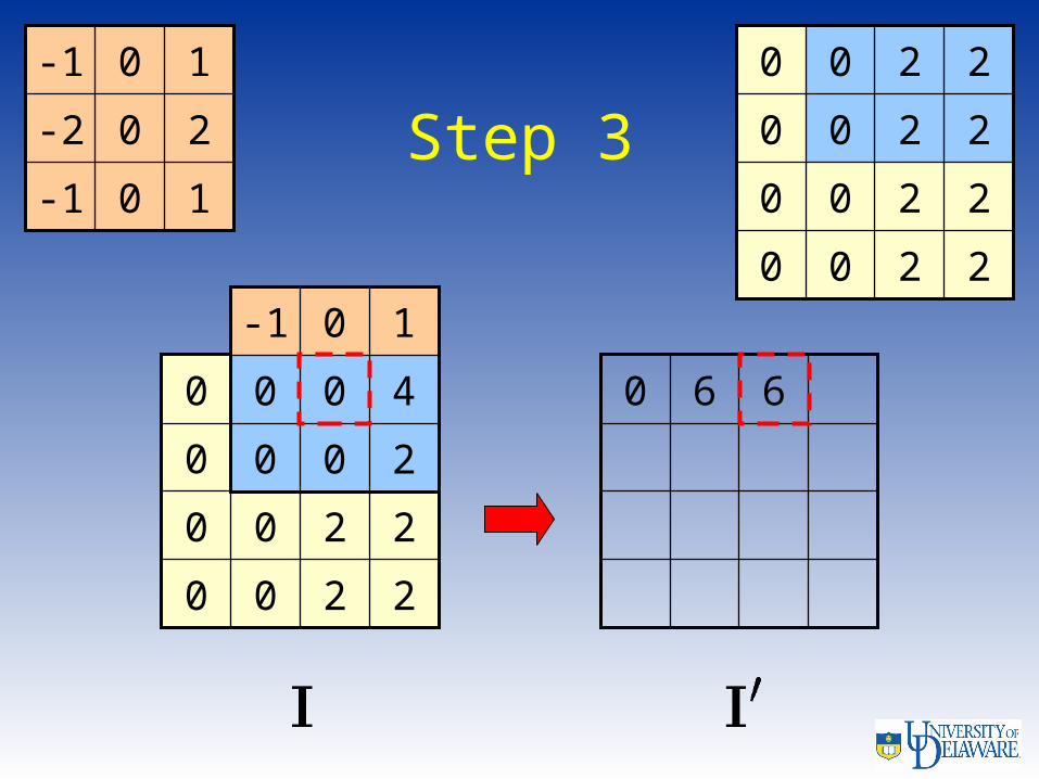
Step 3

0

0

1

2

2

2

3

2

30

20

20

30 6 60

0

0

0

0

2

2

2

2

20

20

20

20

200

400

10-1

10-1

20-2

10-1

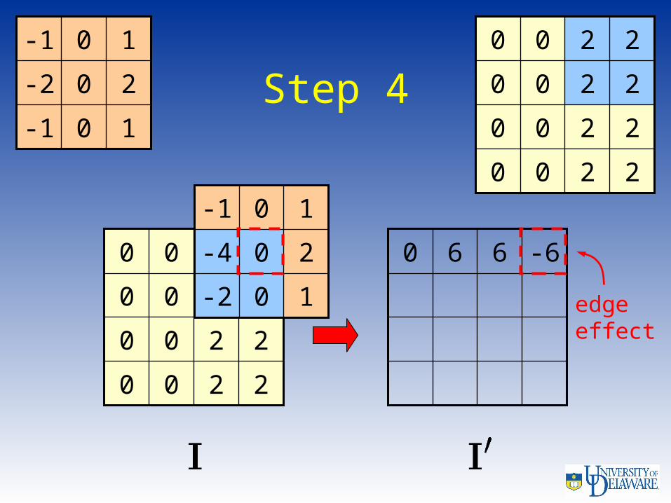
Step 4

0

0

0

0

2

2

3

2

30

20

20

30 6 6 -60

0

0

0

0

2

2

2

2

20

20

20

20

10-2

20-4

10-1

10-1

20-2

10-1

edgeeffect

Sobel Edge Detection: Gradient Approximation

Horizontal Vertical

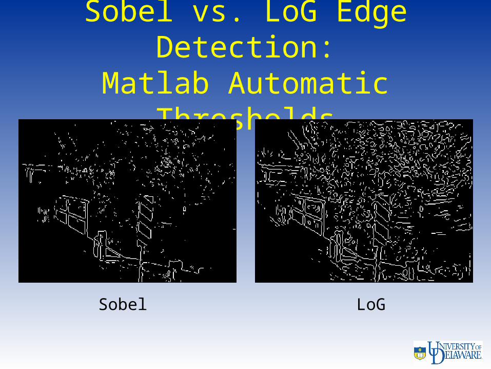
Sobel vs. LoG Edge Detection:

Matlab Automatic Thresholds

Sobel LoG

Canny Edge Detection

• Derivative of Gaussian• Non-maximum suppression

– Thin multi-pixel wide “ridges” down to single pixel

• Thresholding– Low, high edge-strength thresholds– Accept all edges over low threshold that are

connected to edge over high threshold

• Matlab: edge(I, ‘canny’)

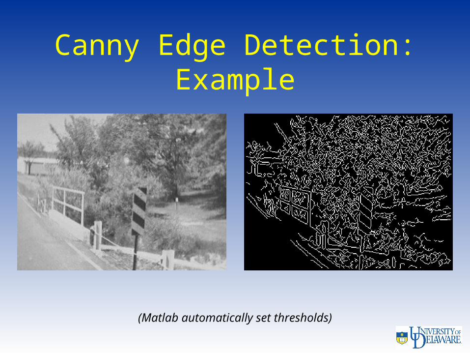
Canny Edge Detection: Example

(Matlab automatically set thresholds)

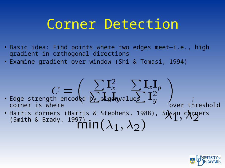
Corner Detection

• Basic idea: Find points where two edges meet—i.e., high gradient in orthogonal directions

• Examine gradient over window (Shi & Tomasi, 1994)

• Edge strength encoded by eigenvalues ; corner is where over threshold

• Harris corners (Harris & Stephens, 1988), Susan corners (Smith & Brady, 1997)

Example: Corner Detection

courtesy of S. Smith

SUSAN corners

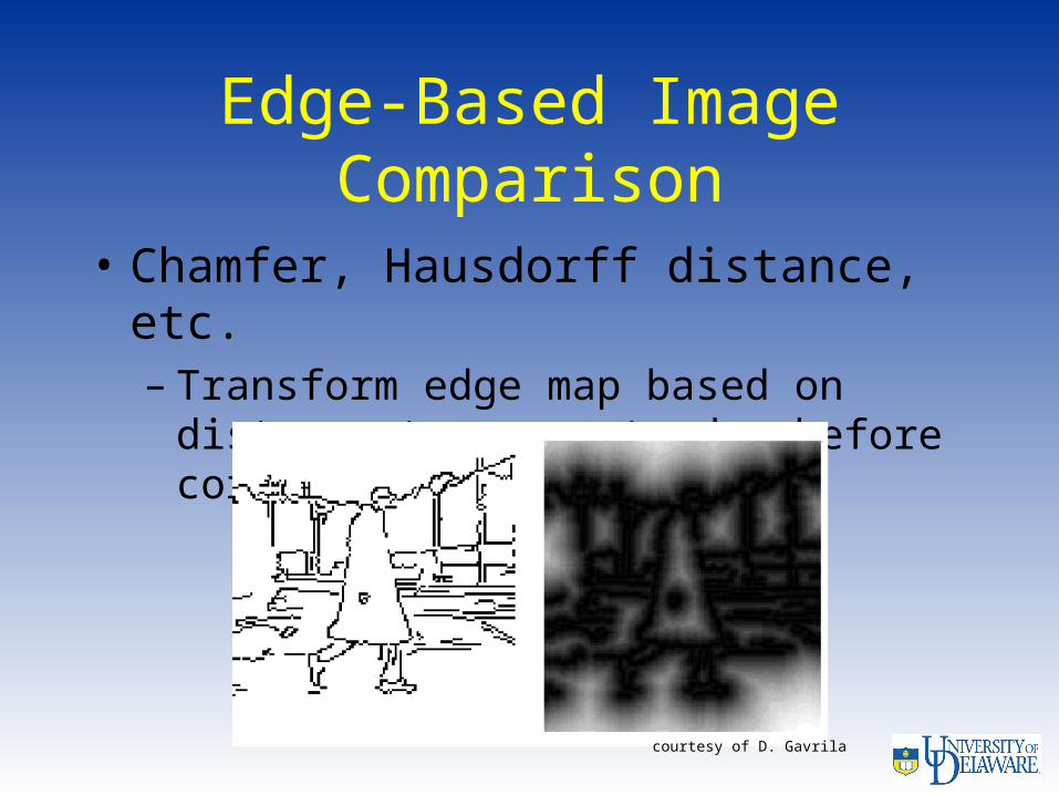
Edge-Based Image Comparison

• Chamfer, Hausdorff distance, etc. – Transform edge map based on

distance to nearest edge before correlating as usual

courtesy of D. Gavrila

Scale Space

• How thick an edge? How big a dot?

• Must consider what scale we are interested in when designing filters

• Efficiency a major consideration: Fine-grained template matching is expensive over a full image

Image Pyramids

• Idea: Represent image at different scales, allowing efficient coarse-to-fine search

• Downsampling: • Simplest scale change: Decimation—

just downsample

from Forsyth & Ponce

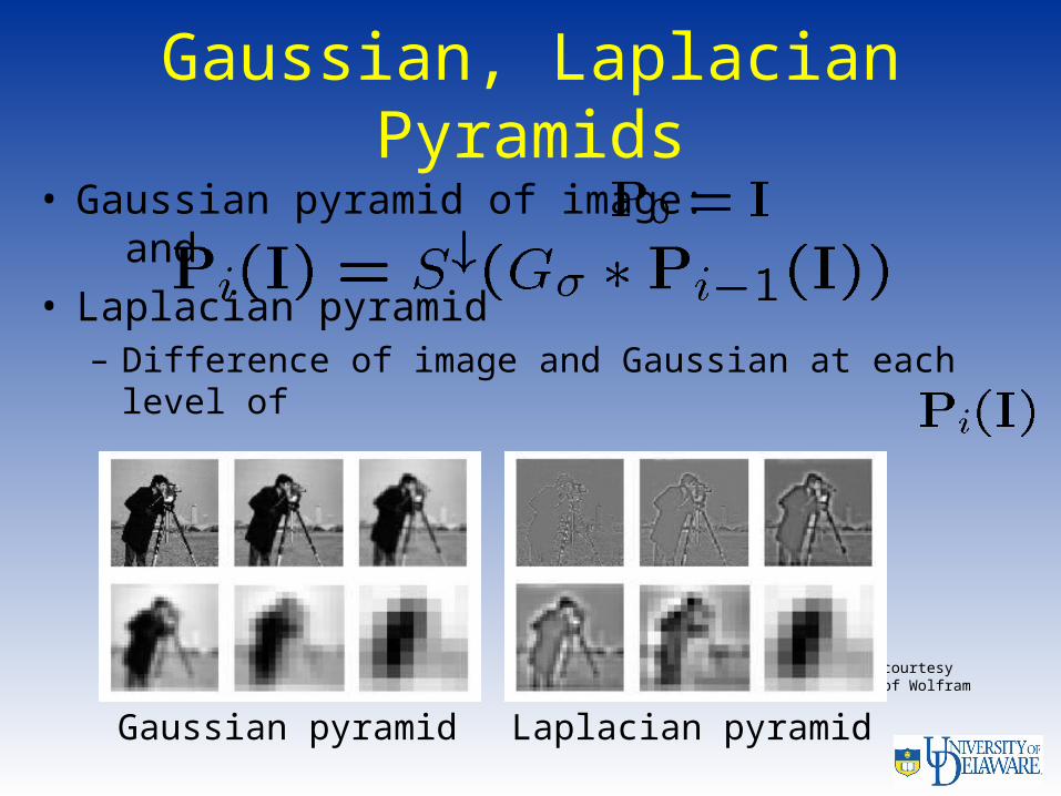
Gaussian, Laplacian Pyramids

• Gaussian pyramid of image: and

• Laplacian pyramid – Difference of image and Gaussian at each level of

courtesy of Wolfram

Gaussian pyramid Laplacian pyramid

Color-based Image Comparison

• Color histograms (Swain & Ballard, 1991)– Steps

• Histogram RGB/HSV triplets over two images to be compared

• Normalize each histogram by respective total number of pixels to get frequencies

• Similarity is Euclidean distance between color frequency vectors

– Sensitive to lighting changes– Works for different-sized images– Matlab: imhist, hist