Embed Size (px)
Citation preview

313
CHAPTER 8
Vision Pipelines and Optimizations
“More speed, less haste . . . ”
—Treebeard, Lord of the Rings
This chapter explores some hypothetical computer vision pipeline designs to understand HW/SW design alternatives and optimizations. Instead of looking at isolated computer vision algorithms, this chapter ties together many concepts into complete vision pipelines. Vision pipelines are sketched out for a few example applications to illustrate the use of different methods. Example applications include object recognition using shape and color for automobiles, face detection and emotion detection using local features, image classification using global features, and augmented reality. The examples have been chosen to illustrate the use of different families of feature description metrics within the Vision Metrics Taxonomy presented in Chapter 5. Alternative optimizations at each stage of the vision pipeline are explored. For example, we consider which vision algorithms run better on a CPU versus a GPU, and discuss how data transfer time between compute units and memory affects performance.
Note ■ The hypothetical examples in this chapter are sometimes sketchy, not intended to be complete. Rather, the intention is to explore design alternatives. Design choices are made in the examples for illustration only; other, equally valid design choices could be made to build working systems. The reader is encouraged to analyze the examples to find weaknesses and alternatives. If the reader can improve the examples, we have succeeded.
This chapter addresses the following major topics, in this order:
1. General design concepts for optimization across the SOC (CPU, GPU, memory).
2. Four hypothetical vision pipeline designs using different descriptor methods.
3. Overview of SW optimization resources and specific optimization techniques.
CHAPTER 8 ■ VISION PIPELINES AND OPTIMIZATIONS
314
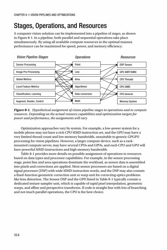
Stages, Operations, and Resources A computer vision solution can be implemented into a pipeline of stages, as shown in Figure 8-1 . In a pipeline, both parallel and sequential operations take place simultaneously. By using all available compute resources in the optimal manner, performance can be maximized for speed, power, and memory efficiency.
Sensor Processing
Image Pre-Processing
Global Metrics
Local Feature Metrics
Classification, Learning
Augment, Render, Control
Vision Pipeline Stages Operations
Point
Line
Area
Algorithmic
Data conversion
DSP Sensor
GPU SIMT/SIMD
CPU Threads
CPU SIMD
CPU General
Memory System
Resources
Math
Figure 8-1. Hypothetical assignment of vision pipeline stages to operations and to compute resources. Depending on the actual resource capabilities and optimization targets for power and performance, the assignments will vary
Optimization approaches vary by system. For example, a low-power system for a mobile phone may not have a rich CPU SIMD instruction set, and the GPU may have a very limited thread count and low memory bandwidth, unsuitable to generic GPGPU processing for vision pipelines. However, a larger compute device, such as a rack-mounted compute server, may have several CPUs and GPUs, and each CPU and GPU will have powerful SIMD instructions and high memory bandwidth.
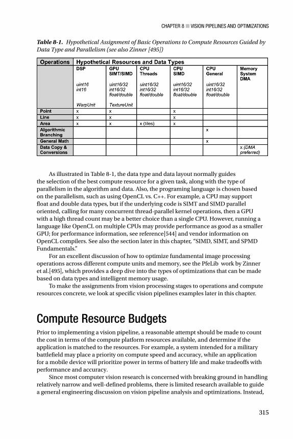
Table 8-1 provides more details on possible assignment of operations to resources based on data types and processor capabilities. For example, in the sensor processing stage, point line and area operations dominate the workload, as sensor data is assembled into pixels and corrections are applied. Most sensor processors are based on a digital signal processor (DSP) with wide SIMD instruction words, and the DSP may also contain a fixed-function geometric correction unit or warp unit for correcting optics problems like lens distortion. The Sensor DSP and the GPU listed in Table 8-1 typically contain a dedicated texture sampler unit, which is capable of rapid pixel interpolation, geometric warps, and affine and perspective transforms. If code is straight line with lots of branching and not much parallel operations, the CPU is the best choice.
CHAPTER 8 ■ VISION PIPELINES AND OPTIMIZATIONS
315
As illustrated in Table 8-1 , the data type and data layout normally guides the selection of the best compute resource for a given task, along with the type of parallelism in the algorithm and data. Also, the programing language is chosen based on the parallelism, such as using OpenCL vs. C++. For example, a CPU may support float and double data types, but if the underlying code is SIMT and SIMD parallel oriented, calling for many concurrent thread-parallel kernel operations, then a GPU with a high thread count may be a better choice than a single CPU. However, running a language like OpenCL on multiple CPUs may provide performance as good as a smaller GPU; for performance information, see reference[544] and vendor information on OpenCL compilers. See also the section later in this chapter, “SIMD, SIMT, and SPMD Fundamentals.”
For an excellent discussion of how to optimize fundamental image processing operations across different compute units and memory, see the PfeLib work by Zinner et al.[495], which provides a deep dive into the types of optimizations that can be made based on data types and intelligent memory usage.
To make the assignments from vision processing stages to operations and compute resources concrete, we look at specific vision pipelines examples later in this chapter.
Compute Resource Budgets Prior to implementing a vision pipeline, a reasonable attempt should be made to count the cost in terms of the compute platform resources available, and determine if the application is matched to the resources. For example, a system intended for a military battlefield may place a priority on compute speed and accuracy, while an application for a mobile device will prioritize power in terms of battery life and make tradeoffs with performance and accuracy.
Since most computer vision research is concerned with breaking ground in handling relatively narrow and well-defined problems, there is limited research available to guide a general engineering discussion on vision pipeline analysis and optimizations. Instead,
Table 8-1. Hypothetical Assignment of Basic Operations to Compute Resources Guided by Data Type and Parallelism (see also Zinner [495])

CHAPTER 8 ■ VISION PIPELINES AND OPTIMIZATIONS
316
we follow a line of thinking that starts with the hardware resources themselves, and we discuss performance, power, memory, and I/O requirements, with some references to the literature for parallel programming and other code-optimization methods. Future research into automated tools to measure algorithm intensity, such as the number of integer and float operations, the bit precision of data types, and the number of memory transfers for each algorithm in terms of read/write, would be welcomed by engineers for vision pipeline analysis and optimizations.
As shown in Figure 8-2 , the main elements of a computer system are composed of I/O, compute, and memory.
Figure 8-2. Hypothetical computer system, highlighting compute elements in the form of a DSP, GPU, four CPU cores, DMA, and memory architecture using L1 and L2 cache and register files RF within each compute unit
We assume suitable high bandwidth I/O busses and cache lines interconnecting the various compute units to memory; in this case, we call out the MIPI camera interface in particular, which connects directly to the DSP in our hypothetical SOC. In the case of a simple computer vision system of the near future, we assume that the price, performance, and power curves continue in the right direction to enable a system-on-a-chip (SOC) sufficient for most computer vision applications to be built at a low price point, approaching throw-away computing cost—similar in price to any small portable electronic gadget. This would thereby enable low-power and high-performance ubiquitous vision applications without resorting to special-purpose hardware accelerators built for any specific computer vision algorithms.
CHAPTER 8 ■ VISION PIPELINES AND OPTIMIZATIONS
317
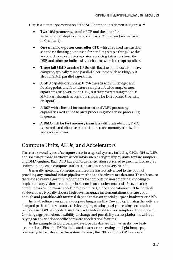
Here is a summary description of the SOC components shown in Figure 8-2 :
• Two 1080p cameras , one for RGB and the other for a self-contained depth camera, such as a TOF sensor (as discussed in Chapter 1).
• One small low-power controller CPU with a reduced instruction set and no floating point, used for handling simple things like the keyboard, accelerometer updates, servicing interrupts from the DSP, and other periodic tasks, such as network interrupt handlers.
• Three full SIMD capable CPUs with floating point, used for heavy compute, typically thread parallel algorithms such as tiling, but also for SIMD parallel algorithms.
• A GPU capable of running ➤ 256 threads with full integer and floating point, and four texture samplers. A wide range of area algorithms map well to the GPU, but the programming model is SIMT kernels such as compute shaders for DirectX and OpenGL, or OpenCL.
• A DSP with a limited instruction set and VLIW processing capabilities well suited to pixel processing and sensor processing in general.
• A DMA unit for fast memory transfers; although obvious, DMA is a simple and effective method to increase memory bandwidth and reduce power.
Compute Units, ALUs, and Accelerators There are several types of compute units in a typical system, including CPUs, GPUs, DSPs, and special-purpose hardware accelerators such as cryptography units, texture samplers, and DMA engines. Each ALU has a different instruction set tuned to the intended use, so understanding each compute unit’s ALU instruction set is very helpful.
Generally speaking, computer architecture has not advanced to the point of providing any standard vision pipeline methods or hardware accelerators. That’s because there are so many algorithm refinements for computer vision emerging; choosing to implement any vision accelerators in silicon is an obsolescence risk. Also, creating computer vision hardware accelerators is difficult, since applications must be portable. So developers typically choose high-level language implementations that are good enough and portable, with minimal dependencies on special purpose hardware or API’s.
Instead, reliance on general-purpose languages like C++ and optimizing the software is a good path to follow to start, as is leveraging existing pixel-processing acceleration methods in a GPU as needed, such as pixel shaders and texture samplers. The standard C++ language path offers flexibility to change and portability across platforms, without relying on any vendor-specific hardware acceleration features.
In the example vision pipelines developed in this section, we make two basic assumptions. First, the DSP is dedicated to sensor processing and light image pre-processing to load-balance the system. Second, the CPUs and the GPUs are used

CHAPTER 8 ■ VISION PIPELINES AND OPTIMIZATIONS
318
downstream for subsequent sections of the vision pipeline, so the choice of CPU vs. GPU depends on the algorithm used.
Since the compute units with programmable ALUs are typically where all the tools and attention for developers are focused, we dedicate some attention to programming acceleration alternatives later in this chapter in the “Vision Algorithm Optimizations and Tuning” section; there is also a survey of selected optimization resources and software building blocks.
In the hypothetical system shown in Figure 8-2 , the compute units include general-purpose CPUs, a GPU intended primarily for graphics and media acceleration and some GPGPU acceleration, and a DSP for sensor processing. Each compute unit is programmable and contains a general-purpose ALU with a tuned instruction set. For example, a CPU contains all necessary instructions for general programming, and may also contain SIMD instructions (discussed later in this chapter). A GPU contains transcendental instructions such as square root, arctangent, and related instructions to accelerate graphics processing. The DSP likewise has an instruction set tuned for sensor processing, likely a VLIW instruction set.
Hardware accelerators are usually built for operations that are common, such as a geometric correction unit for sensor processing in the DSP and texture samplers for warping surface patches in the GPU. There are no standards yet for computer vision, and new algorithm refinements are being developed constantly, so there is little incentive to add any dedicated silicon for computer vision accelerators, except for embedded and special-purpose systems. Instead, finding creative methods of using existing accelerators may prove beneficial.
Later in this chapter we discuss methods for optimizing software on various compute units, taking advantage of the strengths and intended use of each ALU and instruction set.
Power Use It is difficult to quantify the amount of power used for a particular algorithm on an SOC or a single compute device without very detailed power analysis; likely simulation is the best method. Typically, systems engineers developing vision pipelines for an SOC do not have accurate methods of measuring power, except crude means such as running the actual finished application and measuring wall power or battery drain.
The question of power is sometimes related to which compute device is used, such as CPU vs. GPU, since each device has a different gate count and clock rate, therefore is burning power at a different rate. Since silicon architects for both GPU and CPU designs are striving to deliver the most performance per watt per square millimeter , (and we assume that each set of silicon architects is equally efficient), there is no clear winner in the CPU vs. GPU power/performance race. The search to save power by using the GPU vs. the CPU might not even be worth the effort compared to other places to look, such as data organization and memory architecture.
One approach for making the power and performance tradeoff in the case of SIMD and SIMT parallel code is to use a language such as OpenCL, which supports running the same code on either a CPU or a GPU. The performance and power would then need to be measured on each compute device to quantify actual power and performance; there’s more discussion on this topic later, in the “Vision Algorithm Optimizations and Tuning” section.
CHAPTER 8 ■ VISION PIPELINES AND OPTIMIZATIONS
319
For detailed performance analysis using the same OpenCL code running on a specific CPU vs. a GPU, as well as clusters, see the excellent research by the National Center for Super Computing Applications[544]. Also, see the technical computing resources provided by major OpenCL vendors, such as INTEL, NVIDIA, and AMD, for details on their OpenCL compilers running the same code across the CPU vs. GPU. Sometimes the results are surprising, especially for multi-core CPU systems vs. smaller GPUs.
In general, the compute portion of the vision pipeline is not where the power is burned anyway; most power is burned in the memory subsystem and the I/O fabric, where high data bandwidth is required to keep the compute pipeline elements full and moving along. In fact, all the register files, caches, I/O busses, and main memory consume the lion’s share of power and lots of silicon real estate. So memory use and bandwidth are high-value targets to attack in any attempt to reduce power. The fewer the memory copies, the higher the cache hit rates; the more reuse of the same data in local register files, the better.
Memory Use Memory is the most important resource to manage as far as power and performance are concerned. Most of the attention on developing a vision pipeline is with the algorithms and processing flow, which is challenging enough. However, vision applications are highly demanding of the memory system. The size of the images alone is not so great, but when we consider the frame rates and number of times a pixel is read or written for kernel operations through the vision pipeline, the memory transfer bandwidth activity becomes clearer. The memory system is complex, consisting of local register files next to each compute unit, caches, I/O fabric interconnects, and system memory. We look at several memory issues in this section, including:
Pixel resolution, bit precision, and total image size •
Memory transfer bandwidth in the vision pipeline •
Image formats, including gray scale and color spaces •
Feature descriptor size and type •
Accuracy required for matching and localization •
Feature descriptor database size •
To explore memory usage, we go into some detail on a local interest point and feature extraction scenario, assuming that we locate interest points first, filter the interest points against some criteria to select a smaller set, calculate descriptors around the chosen interest points, and then match features against a database.
A reasonable first estimate is that between a lower bound and upper bound of 0.05% to 1 percent of the pixels in an image can generate decent interest points. Of course, this depends entirely on: (1) the complexity of the image texture, and (2) the interest point method used. For example, an image with rich texture and high contrast will generate more interest points than an image of a far away mountain surrounded by clouds with little texture and contrast. Also, interest point detector methods yield different results—for example, the FAST corner method may detect more corners than a SIFT scale invariant DoG feature, see Appendix A.

CHAPTER 8 ■ VISION PIPELINES AND OPTIMIZATIONS
320
Descriptor size may be an important variable, see Table 8-2 . A 640x480 image will contain 307,200 pixels. We estimate that the upper bound of 1 percent, or 3,072 pixels, may have decent interests points; and we assume that the lower bound of 0.05 percent is 153. We provide a second estimate that interest points may be further filtered to sort out the best ones for a given application. So if we assume perhaps only as few as 33 percent of the interest points are actually kept, then we can say that between 153*.33 and 3,072*.33 interest points are good candidates for feature description. This estimate varies widely out of bounds, depending of course on the image texture, interest point method used, and interest point filtering criteria. Assuming a feature descriptor size is 256 bytes, the total descriptor size per frame is 3072x256x.33 = 259,523 bytes maximum—that’s not extreme. However, when we consider the feature match stage, the feature descriptor count and memory size will be an issue, since each extracted feature must be matched against each trained feature set in the database.
Table 8-2. Descriptor Bytes per Frame (1% Interest Points), adapted from [141]
Descriptor Size in bytes 480p NTSC 1080p HD 2160p 4kUHD 4320p 8kUHD
Resolution 640 x 480 1920 x 1080 3840 × 2160 7680 x 4320
Pixels 307200 2073600 8294400 33177600
BRIEF 32 98304 663552 2654208 10616832
ORB 32 98304 663552 2654208 10616832
BRISK 64 196608 1327104 5308416 21233664
FREAK (4 cascades)
64 196608 1327104 5308416 21233664
SURF 64 196608 1327104 5308416 21233664
SIFT 128 393216 2654208 10616832 42467328
LIOP 144 442368 2985984 11943936 47775744
MROGH 192 589824 3981312 15925248 63700992
MRRID 256 786432 5308416 21233664 84934656
HOG (64x128 block)
3780 n.a. n.a. n.a. n.a.
In general, local binary descriptors offer the advantage of a low memory footprint. For example, Table 8-2 provides the byte count of several descriptors for comparison, as described in Miksik and Mikolajczyk [141]. The data is annotated here to add the descriptor working memory size in bytes per frame for various resolutions.
In Table 8-2 , image frame resolutions are in row 1, pixel count per frame is in row 2, and typical descriptor sizes in bytes are in subsequent rows. Total bytes for selected descriptors are in column 1, and the remaining columns show total descriptor size per

CHAPTER 8 ■ VISION PIPELINES AND OPTIMIZATIONS
321
frame assuming an estimated 1 percent of the pixels in each frame are used to calculate an interest point and descriptor. In practice, we estimate that 1 percent is an upper-bound estimate for a descriptor count per frame and 0.05 percent is a lower-bound estimate. Note that descriptor sizes in bytes do vary from those in the table, based on design optimizations.
Memory bandwidth is often a hidden cost, and often ignored until the very end of the optimization cycle, since developing the algorithms is usually challenging enough without also worrying about the memory access patterns and memory traffic. Table 8-2 includes a summary of several memory variables for various image frame sizes and feature descriptor sizes. For example, using the 1080p image pixel count in row 2 as a base, we see that an RGB image with 16 bits per color channel will consume:
2,073,600 pixels
*3 channels/RGB
*2 bytes/pixel
= 12,441,600 bytes / frame
And if we include the need to keep a gray scale channel I around, computed from the RGB, the total size for RGBI increases to:
2,073,600 pixels
*4 channels/RGBI
*2 bytes/pixel
= 16,588,800 bytes / frame
If we then assume 30 frames per second and two RGB cameras for depth processing + the I channel, the memory bandwidth required to move the complete 4-channel RGBI image pair out of the DSP is nearly 1GB / second:
12,441,600 pixels
*4 channels/RGBI
* bytes/pixel
*30 fps
*2 stereo
= 995,328,000 mb/s
So we assume in this example a baseline memory bandwidth of about ~1GB/second just to move the image pair downstream from the ISP. We are ignoring the ISP memory read/write requirements for sensor processing for now, assuming that clever DSP memory caching, register file design, and loop-unrolling methods in assembler can reduce the memory bandwidth.
Typically, memory coming from a register file in a compute unit transfers in a single clock cycle; memory coming from various cache layers can take maybe tens of clock cycles; and memory coming from system memory can take hundreds of clock cycles. During memory transfers, the ALU in the CPU or GPU may be sitting idle, waiting on memory.
Memory bandwidth is spread across the fast register files next to the ALU processors, and through the memory caches and even system memory, so actual memory bandwidth is quite complex to analyze. Even though some memory bandwidth numbers are provided here, it is only to illustrate the activity.
And the memory bandwidth only increases downstream from the DSP, since each image frame will be read, and possibly rewritten, several times during image pre-processing, then also read again during interest point generation and feature extraction. For example, if we assume only one image pre-processing operation using 5x5 kernels on the I channel, each I pixel is read another 25 times, hopefully from memory cache lines and fast registers.
This memory traffic is not all coming from slow-system memory, and it is mostly occurring inside the faster-memory cache system and faster register files until there is a cache miss or reload of the fast-register files. Then, performance drops by an order of

CHAPTER 8 ■ VISION PIPELINES AND OPTIMIZATIONS
322
magnitude waiting for the buffer fetch and register reloading. If we add a FAST9 interest point detector on the I channel, each pixel is read another 81 times (9x9), maybe from memory cache lines or registers. And if we add a FREAK feature descriptor over maybe 0.05 percent of the detected interest points, we add 41x41 pixel reads per descriptor to get the region (plus 45*2 reads for point-pair comparisons within the 41x41 region), hopefully from memory cache lines or registers.
Often the image will be processed in a variety of formats, such as image pre-processing the RGB colors to enhance the image, and conversion to gray scale intensity I for computing interest points and feature descriptors. The color conversions to and from RGB are a hidden memory cost that requires data copy operations and temporary storage for the color conversion, which is often done in floating point for best accuracy. So, several more GB/second of memory bandwidth can be consumed for color conversions. With all the memory activity, there may be cache evictions of all or part of the required images into a slower system memory, degrading into nonlinear performance.
Memory size of the descriptor, therefore, is a consideration throughout the vision pipeline. First, we consider when the features are extracted; and second, we look at when the features are matched and retrieved from the feature database. In many cases, the size of the feature database is by far the critical issue in the area of memory, since the total size of all the descriptors to match against affects the static memory storage size, memory bandwidth, and pattern match rate. Reducing the feature space into a quickly searchable format during classification and training is often of paramount importance. Besides the optimized classification methods discussed in Chapter 4, the data organization problems may be primarily in the areas of standard computer science searching, sorting, and data structures; some discussion and references were provided in Chapter 4.
When we look at the feature database or training set, memory size can be the dominant issue to contend with. Should the entire feature database be kept on a cloud server for matching? Or should the entire feature database be kept on the local device? Should a method of caching portions of the feature database on the local device from the server be used? All of the above methods are currently employed in real systems.
In summary, memory, caches, and register files exceed the silicon area of the ALU processors in the compute units by a large margin. Memory bandwidth across the SOC fabric through the vision pipeline is key to power and performance, demanding fast memory architecture and memory cache arrangement, and careful software design. Memory storage size alone is not the entire picture, though, since each byte needs to be moved around between compute units. So, careful consideration of memory footprint and memory bandwidth is critical for anything but small applications.
Often, performance and power can be dramatically improved by careful attention to memory issues alone. Later in the chapter we cover several design methods to help reduce memory bandwidth and increase memory performance, such as locking pages in memory, pipelining code, loop unrolling, and SIMD methods. Future research into minimizing memory traffic in a vision pipeline is a worthwhile field.
I/O Performance We lump I/O topics together here as a general performance issue, including data bandwidth on the SOC I/O fabric between compute units, image input from the camera, and feature descriptor matching database traffic to a storage device. We touched

CHAPTER 8 ■ VISION PIPELINES AND OPTIMIZATIONS
323
on I/O issues above the discussion on memory, since pixel data is moved between various compute devices along the vision pipeline on I/O busses. One of the major I/O considerations is feature descriptor data moving out of the database at feature match time, so using smaller descriptors and optimizing the feature space using effective machine learning and classification methods is valuable.
Another type of I/O to consider is the camera input itself, which is typically accomplished via the standard MIPI interface. However, any bus or I/O fabric can be used, such as USB. If the vision pipeline design includes a complete HW/SW system design rather than software only on a standard SOC, special attention to HW I/O subsystem design for the camera and possibly special fast busses for image memory transfers to and from a HW-assisted database may be worthwhile. When considering power, I/O fabric silicon area and power exceed the area and power for the ALU processors by a large margin.
The Vision Pipeline Examples In this section we look at four hypothetical examples of vision pipelines. Each is chosen to illustrate separate descriptor families from the Vision Metrics Taxonomy presented in Chapter 5, including global methods such as histograms and color matching, local feature methods such as FAST interest points combined with FREAK descriptors, basis space methods such as Fourier descriptors, and shape-based methods using morphology and whole object shape metrics. The examples are broken down into stages , operations, and resources, as shown in Figure 8-1 , for the following applications:
• Automobile recognition, using shape and color
• Face recognition, using sparse local features
• Image classification, using global features
• Augmented reality, using depth information and tracking
None of these examples includes classification, training, and machine learning details, which are outside the scope of this book (machine learning references are provided in Chapter 4). A simple database storing the feature descriptors is assumed to be adequate for this discussion, since the focus here is on the image pre-processing and feature description stages. After working through the examples and exploring alternative types of compute resource assignments, such as GPU vs. CPU, this chapter finishes with a discussion on optimization resources and techniques for each type of compute resource.
Automobile Recognition Here we devised a vision pipeline to recognize objects such as automobiles or machine parts by using polygon shape descriptors and accurate color matching . For example, polygon shape metrics can be used to measure the length and width of a car, while color matching can be used to measure paint color. In some cases, such as custom car paint jobs, color alone is not sufficient for identification.
For this automobile example, the main design challenges include segmentation of automobiles from the roadway, matching of paint color, and measurement of automobile size and shape. The overall system includes an RGB-D camera system, accurate color

CHAPTER 8 ■ VISION PIPELINES AND OPTIMIZATIONS
324
and illumination models, and several feature descriptors used in concert. See Figure 8-3 . We work through this example in some detail as a way of exploring the challenges and possible solutions for a complete vision pipeline design of this type.
60 feet
RGB-D Camera
Lamp
FOV
44 feet, 11 feet per lane
Figure 8-3. Setting for an automobile identification application using a shape-based and color-based vision pipeline. The RGB and D cameras are mounted above the road surface, looking directly down
We define the system with the following requirements :
1080p RGB color video (1920x1080 pixels) at 120 fps, horizontally • mounted to provide highest resolution in length, 12 bits per color, 65 degree FOV.
1080p stereo depth camera with 8 bits Z resolution at 120 fps, • 65 degree FOV.
Image FOV covering 44 feet in width and 60 feet in length over • four traffic lanes of oncoming traffic, enough for about three normal car lengths in each lane when traffic is stopped.
Speed limit of 25 mph, which equals ~37 feet per second. •
Camera mounted next to overhead stoplight, with a street lamp • for night illumination.

CHAPTER 8 ■ VISION PIPELINES AND OPTIMIZATIONS
325
Embedded PC with 4 CPU cores having SIMD instruction sets, • one GPU, 8GB memory, 80GB disk; assumes high-end PC equivalent performance (not specified for brevity).
Identification of automobiles in real time to determine make and • model; also count of occurrences of each, with time stamp and confidence score.
Automobile ground truth training dataset provided by major • manufacturers to include geometry, and accurate color samples of all body colors used for stock models; custom colors and after-market colors not possible to identify.
Average car sizes ranging from 5 to 6 feet wide and 12 to 16 feet long. •
Accuracy of 99 percent or better. •
Simplified robustness criteria to include noise, illumination, and • motion blur.
Segmenting the Automobiles To segment the automobiles from the roadway surface, a stereo depth camera operating at 1080p 120fps (frames per second) is used, which makes isolating each automobile from the roadway simple using depth. To make this work, a method for calibrating the depth camera to the baseline road surface is developed, allowing automobiles to be identified as being higher than the roadway surface. We sketch out the depth calibration method here for illustration.
Spherical depth differences are observed across the depth map, mostly affecting the edges of the FOV. To correct for the spherical field distortion, each image is rectified using a suitable calibrated depth function (to be determined on-site and analytically), then each horizontal line is processed, taking into consideration the curvilinear true depth distance, which is greater at the edges, to set the depth equal across each line.
Since the speed limit is 25 mph, or 37 feet per second, imaging at 120 FPS yields maximum motion blur of about 0.3 feet, or 4 inches per frame. Since the length of a pixel is determined to be 0.37 inches, as shown in Figure 8-4 , the ability to compute car length from pixels is accurate within about 4 inches/0.37 inches = 11 pixels, or about 3 percent of a 12-foot-long car at 25 mph including motion blur. However, motion blur compensation can be applied during image pre-processing to each RGB and depth image to effectively reduce the motion blur further; several methods exist based on using convolution or compensating over multiple sequential images [305,492].

CHAPTER 8 ■ VISION PIPELINES AND OPTIMIZATIONS
326
Matching the Paint Color We assume that it is possible to identify a vehicle using paint color alone in many cases, since each manufacturer uses proprietary colors, therefore accurate colorimetry can be employed. For matching paint color , 12 bits per color channel should provide adequate resolution, which is determined in the color match stage using the CIECAM02 model and the Jch color space [253]. This requires development of several calibrated device models of the camera with the scene under different illumination conditions, such as full sunlight at different times of day, cloud cover, low light conditions in early morning and at dusk, and nighttime using the illuminator lamp mounted above traffic along with the camera and stop light.
The key to colorimetric accuracy is the device models’ accounting for various lighting conditions. A light sensor to measure color temperature, along with the knowledge of time of day and season of the year, is used to select the correct device models for proper illumination for times of day and seasons of the year. However, dirty cars present problems for color matching; for now we ignore this detail (also custom paint jobs are a problem). In some cases, the color descriptor may not be useful or reliable; in other cases, color alone may be sufficient to identify the automobile. See the discussion of color management in Chapter 2.
Measuring the Automobile Size and Shape For automobile size and shape , the best measurements are taken looking directly down on the car to reduce perspective distortion. As shown in Figure 8-4 , the car is segmented into C (cargo), T (top), and H (hood) regions using depth information from the stereo camera, in combination with a polygon shape segmentation of the auto shape. To compute shape, some weighted combination of RGB and D images into a single image will be used, based on best results during testing. We assume the camera is mounted in the best possible location centered above all lanes, but that some perspective distortion will exist at the far ends of the FOV. We also assume that a geometric correction is applied to rectify the images into Cartesian alignment. Assuming errors introduced by
Mirror
Length
WidthC T H
Figure 8-4. Features used for automobile identification

CHAPTER 8 ■ VISION PIPELINES AND OPTIMIZATIONS
327
the geometric corrections to rectify the FOV are negligible, the following approximate dimensional precision is expected for length and width, using the minimum car size of 5’ x 12’ as an example:
FOV Pixel Width: 1080pixels
/ (44’ * 12”)inches
= each pixel is ~0.49 inches wide FOV Pixel Length: 1920
pixels / (60’ * 12”)
inches = each pixel is ~0.37 inches long
Automobile Width: (5’ * 12”) / .49 = ~122 pixels Automobile Length: (12’ * 12”) / .37 = ~389 pixels
This example uses the following shape features :
Bounding box containing all features; width and length are used •
Centroid computed in the middle of the automobile region •
Separate width computed from the shortest diameter passing • through the centroid to the perimeter
Mirror feature measured as the distance from the front of the car; • mirror locations are the smallest and largest perimeter width points within the bounding box
Shape segmented into three regions using depth; color is measured • in each region: cargo compartment (C), top (T), and hood (H)
Fourier descriptor of the perimeter shape computed by • measuring the line segments from centroid to perimeter points at intervals of 5 degrees
Feature Descriptors Several feature descriptors are used together for identification, and the confidence of the automobile identification is based on a combined score from all descriptors. The key feature descriptors to be extracted are as follows:
• Automobile shape factors: Depth-based segmentation of each automobile above the roadway is used for the coarse shape outline. Some morphological processing follows to clean up the edges and remove noise. For each segmented automobile, object shape factors are computed for area, perimeter, centroid, bounding box, and Fourier descriptors of perimeter shape. The bounding box measures overall width and height, the Fourier descriptor measures the roundness and shape factors; some automobiles are more boxy, some are more curvy. (See Figure 6-32, Figure 2-18, and Chapter 6 for more information on shape descriptors. See Chapter 1 for more information on depth sensors.) In addition, the distance of the mirrors from the front of the automobile is computed; mirrors are located at width extrema around the object perimeter, corresponding to the width of the bounding box.

CHAPTER 8 ■ VISION PIPELINES AND OPTIMIZATIONS
328
• Automobile region segmentation : Further segmentation uses a few individual regions of the automobile based on depth, namely the hood, roof, and trunk. A simple histogram is created to gather the depth statistical moments, a clustering algorithm such as K-means is performed to form three major clusters of depth: the roof will be highest, hood and trunk will be next highest, windows will be in between (top region is missing for convertibles, not covered here). The pixel areas of the hood, top, trunk, and windows are used as a descriptor.
• Automobile color : The predominant colors of the segmented hood, roof, and trunk regions are used as a color descriptor. The colors are processed in the Jch color space, which is part of the CIECAM system yielding high accuracy. The dominant color information is extracted from the color samples and normalized against the illumination model. In the event of multiple paint colors, separate color normalization occurs for each. (See Chapter 3 for more information on colorimetry.)
Calibration , Set-up, and Ground Truth Data Several key assumptions are made regarding scene set-up, camera calibration, and other corrections; we summarize them here:
• Roadway depth surface: Depth camera is calibrated to the road surface as a reference to segment autos above the road surface; a baseline depth map with only the road is calibrated as a reference and used for real-time segmentation.
• Device models: Models for each car are created from manufacturer’s information, with accurate body shape geometry and color for each make and model. Cars with custom paint confuse this approach; however, the shape descriptor and the car region depth segmentation provide a failsafe option that may be enough to give a good match—only testing will tell for sure.
• Illumination models: Models are created for various conditions, such as morning light, daylight, and evening light, for sunny and cloudy days; illumination models are selected based on time of day and year and weather conditions for best matching.
• Geometric model for correction: Models of the entire FOV for both the RGB and depth camera are devised, to be applied at each new frame to rectify the image.

CHAPTER 8 ■ VISION PIPELINES AND OPTIMIZATIONS
329
Pipeline Stages and Operations Assuming the system is fully calibrated in advance, the basic real-time processing flow for the complete pipeline is shown in Figure 8-5 , divided into three primary stages of operations. Note that the complete pipeline includes an image pre-processing stage to align the image in the FOV and segment features, a feature description stage to compute shape and color descriptors, and a correspondence stage for feature matching to develop the final automobile label composed of a weighted combination of shape and color features. We assume that a separate database table for each feature in some standard database is fine.
No attempt is made to create an optimized classifier or matching stage here; instead, we assume, without proving or testing, that a brute-force search using a standard database through a few thousand makes and models of automobile objects works fine for the ALPHA version.
Note in Figure 8-5 (bottom right) that each auto is tracked from frame to frame, we do not define the tracking method here.
Capture RGB and D images
Rectify FOV using 4-point warp, merge RGB and D
Remove motion blur via spatio-temporal merging
Segment shape regions (T,H,C) w/depth+color
Morphological processing to clean up shape
Segment roadway from automobile using depth
Compute perimeter, area, centroid, bounding box
Compute radius lines, centroid to perimeter
Compute radius length histogram, normalized
Compute Fourier Descriptor from radial
Compute mirror distance from front of automobile
Compute dominant color of each automobile shape
Classify features
Bounding Box
Dominant Color
Mirror Distance
Radius Histogram
Fourier Descriptor
Object classification score + tracking
Image pre-processing Feature Description Correspondence
Figure 8-5. Operations in hypothetical vision pipeline for automobile identification using polygon shape features and color

CHAPTER 8 ■ VISION PIPELINES AND OPTIMIZATIONS
330
Operations and Compute Resources For each operation in the pipeline stages, we now explore possible mappings to the available compute resources. First, we review the major resources available in our example system, which contains 8GB of fast memory, we assume sufficient free space to map and lock the entire database in memory to avoid paging. Our system contains four CPU cores, each with SIMD instruction sets, and a GPU capable of running 128 SIMT threads simultaneously with 128GB/s memory bandwidth to shared memory for the GPU and CPU, considered powerful enough. Let’s assume that, overall, the compute and memory resources are fine for our application and no special memory optimizations need to be considered. Next, we look at the coarse-grain optimizations to assign operations to compute resources. Table 8-3 provides an evaluation of possible resource assignments.
Table 8-3. Assignment of Operations to Compute Resources
Criteria for Resource Assignments In our simple example, as shown in Table 8-3 , the main criteria for assigning algorithms to compute units are processor suitability and load balancing among the processors; power is not an issue for this application. The operation to resource assignments provided in Figure 8-5 are a starting point in this hypothetical design exercise; actual optimizations would be different, adjusted based on performance profiling. However, assuming what is obvious about the memory access patterns used for each algorithm, we can make a good guess at resource assignments based on memory access patterns. In a second-order analysis, we could also look at load balancing across the pipeline to maximize parallel uses of compute units; however, this requires actual performance measurements.

CHAPTER 8 ■ VISION PIPELINES AND OPTIMIZATIONS
331
Here we will tentatively assign the tasks from Table 8-3 to resources. If we look at memory access patterns, using the GPU for the sequential tasks 2 and 3 makes sense, since we can map the images into GPU memory space first and then follow with the three sequential operations using the GPU. The GPU has a texture sampler to which we assign task 2, the geometric corrections using the four-point warp. Some DSPs or camera sensor processors also have a texture sampler capable of geometric corrections, but not in our example. In addition to geometric corrections, motion blur is a good candidate for the GPU as well, which can be implemented as an area operation efficiently in a shader. For higher-end GPUs, there may even be hardware acceleration for motion blur compensation in the media section.
Later in the pipeline, after the image has been segmented in tasks 4 and 5, the morphology stage in task 6 can be performed rapidly using a GPU shader; however, the cost of moving the image to and from the GPU for the morphology may actually be slower than performing the morphology on the CPU, so performance analysis is required for making the final design decision regarding CPU vs. GPU implementation.
In the case of stages 7 to 11, shown in Table 8-3 , the algorithm for area, perimeter, centroid, and other measurements span a nonlocalized data access pattern. For example, perimeter tracing follows the edge of the car. So we will make one pass using a single CPU through the image to track the perimeter and compute the area, centroid, and bounding box for each automobile. Then, we assign each bounding box as an image tile to a separate CPU thread for computation of the remaining measurements: radial line segment length, Fourier descriptor, and mirror distance. Each bounding box is then assigned to a separate CPU thread for computation of the colorimetry of each region, including cargo, roof, and hood, as shown in Table 8-3 . Each CPU thread uses C++ for the color conversions and attempts to use compiler flags to force SIMD instruction optimizations.
Tracking the automobile from frame to frame is possible using shape and color features; however, we do not develop the tracking algorithm here. For correspondence and matching, we rely on a generic database from a third party, running in a separate thread on a CPU that is executing in parallel with the earlier stages of the pipeline. We assume that the database can split its own work into parallel threads. However, an optimization phase later could rewrite and create a better database and classifier, using parallel threads to match feature descriptors.
Face, Emotion, and Age Recognition In this example, we design a face, emotion, and age recognition pipeline that uses local feature descriptors and interest points. Face recognition is concerned with identifying the unique face of a unique person, while face detection is concerned with determining only where a face is located and interesting characteristics such as emotion, age, and gender. Our example is for face detection, and finding the emotions and age of the subject.
For simplicity, this example uses mugshots of single faces taken with a stationary camera for biometric identification to access a secure area. Using mugshots simplifies the example considerably, since there is no requirement to pick out faces in a crowd from many angles and distances. Key design challenges include finding a reliable interest point and feature descriptor method to identify the key facial landmarks, determining emotion and age, and modeling the landmarks in a normalized, relative coordinate system to allow for distance ratios and angles to be computed.
CHAPTER 8 ■ VISION PIPELINES AND OPTIMIZATIONS
332
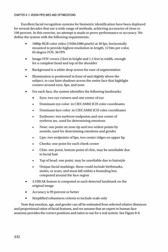
Excellent facial recognition systems for biometric identification have been deployed for several decades that use a wide range of methods, achieving accuracies of close to 100 percent. In this exercise, no attempt is made to prove performance or accuracy. We define the system with the following requirements :
1080p RGB color video (1920x1080 pixels) at 30 fps, horizontally • mounted to provide highest resolution in length, 12 bits per color, 65 degree FOV, 30 FPS
Image FOV covers 2 feet in height and 1.5 feet in width, enough • for a complete head and top of the shoulder
Background is a white drop screen for ease of segmentation •
Illumination is positioned in front of and slightly above the • subject, to cast faint shadows across the entire face that highlight corners around eyes, lips, and nose
For each face, the system identifies the following landmarks:•
Eyes: two eye corners and one center of eye •
Dominant eye color: in CIECAM02 JCH color coordinates •
Dominant face color: in CIECAM02 JCH color coordinates •
Eyebrows: two eyebrow endpoints and one center of • eyebrow arc, used for determining emotions
Nose: one point on nose tip and two widest points by • nostrils, used for determining emotions and gender
Lips: two endpoints of lips, two center ridges on upper lip •
Cheeks: one point for each cheek center •
Chin: one point, bottom point of chin, may be unreliable due • to facial hair
Top of head: one point; may be unreliable due to hairstyle •
Unique facial markings: these could include birthmarks, • moles, or scars, and must fall within a bounding box computed around the face region
A FREAK feature is computed at each detected landmark on the • original image
Accuracy is 99 percent or better •
Simplified robustness criteria to include scale only •
Note that emotion, age, and gender can all be estimated from selected relative distances and proportional ratios of facial features, and we assume that an expert in human face anatomy provides the correct positions and ratios to use for a real system. See Figure 8-6 .

CHAPTER 8 ■ VISION PIPELINES AND OPTIMIZATIONS
333
The set of features computed for this example system includes:
1. Relative positions of facial landmarks such as eyes, eyebrows, nose, and mouth
2. Relative proportions and ratios between landmarks to determine age, sex, and emotion
3. FREAK descriptor at each landmark
4. Eye color
Calibration and Ground Truth Data The calibration is simple: a white backdrop is used in back of the subject, who stands about 4 feet away from the camera, enabling a shot of the head and upper shoulders. (We discuss the operations used to segment the head from the background region later in this section.) Given that we have a 1080p image, we allocate the 1920 pixels to the vertical direction and the 1080 pixels to the horizontal.
Assuming the cameraman is good enough to center the head in the image so that the head occupies about 50 percent of the horizontal pixels, and about 50 percent of the vertical pixels, we have pixel resolution for the head of ~540 pixels horizontal and ~960 pixels vertical, which is good enough for our application and corresponds to the ratio of head height to width. Since we assume that average head height is about 9 inches and width as 6 inches across for male and female adults, using our assumptions for a four-foot distance from the camera, we have plenty of pixel accuracy and resolution:
9” / (1920 pixels
* .5) = 0.009” vertical pixel size
6” / (1080 pixels
* .5) = 0.01” horizontal pixel size
The ground truth data consists of: (1) mugshots of known people, and (2) a set of canonical eye landmark features in the form of correlation templates used to assist in
Figure 8-6. (Left) Proportional ratios based on a bounding box of the head and face regions as guidelines to predict the location of facial landmarks. (Right) Annotated image with detected facial landmark positions and relative angles and distances measured between landmarks. The relative measurements are used to determine emotion, age, and gender

CHAPTER 8 ■ VISION PIPELINES AND OPTIMIZATIONS
334
locating face landmarks (a sparse codebook of correlation temlpates). There are two sets of correlation templates: one for fine features based on a position found using a Hessian detector, and one for coarse features based on a position found using a steerable filter based detector (the fine and coarse detectors are described in more detail later in this example).
Since facial features like eyes and lips are very similar among people, the canonical landmark feature correlation templates provide only rough identification of landmarks and their location. Several templates are provided covering a range of ages and genders for all landmarks, such as eye corners, eyebrow corners, eyebrow peaks, nose corners, nose bottom, lip corners, and lip center region shapes. For sake of brevity, we do not develop the ground truth dataset for correlation templates here, but we assume the process is accomplished using synthetic features created by warping or changing real features and testing them against several real human faces to arrive at the best canonical feature set. The correlation templates are used in the face landmark identification stage, discussed later.
Interest Point Position Prediction To find the facial landmarks, such as eyes, nose, and mouth, this example application is simplified by using mugshots, making the position of facial features predictable and enabling intelligent search for each feature at the predicted locations. Rather than resort to scientific studies of head sizes and shapes, for this example we use basic proportional assumptions from human anatomy (used for centuries by artists) to predict facial feature locations and enable search for facial features at predicted locations. Facial feature ratios differ primarily by age, gender, and race; for example, typical adult male ratios are shown in Table 8-4 .
Table 8-4. Basic Approximate Face and Head Feature Proportions
Head height head width X 1.25
Head width head height X .75
Face height head height X .8
Face width head height X .8
Eye position eye center located 30% in from left/right edges, 50% from top
Eye length head width X 1.25
Eye spacing head width X .5
Nose position 25% higher than lip corners
Nose length head height X .25
Lip corners about eye center x , about 15% higher than chin y
Mouth/lip width head width X .07

CHAPTER 8 ■ VISION PIPELINES AND OPTIMIZATIONS
335
Note ■ The information in Table 8-4 is synthesized for illustration purposes from elementary artists’ materials and is not guaranteed to be accurate.
The most basic coordinates to establish are the bounding box for the head. From the bounding box, other landmark facial feature positions can be predicted.
Segmenting the Head and Face Using the Bounding Box As stated earlier, the mugshots are taken from a distance of about 4 feet against a white drop background, allowing simple segmentation of the head. We use thresholding on simple color intensity as RGBI-I, where I = (R=G + B) / 3 and the white drop background is identified as the highest intensity.
The segmented head and shoulder region is used to create a bounding box of the head and face, discussed next. (Note: wild hairstyles will require another method, perhaps based on relative sizes and positions of facial features compared to head shape and proportions.) After segmenting the bounding box for the head, we proceed to segment the facial region and then find each landmark. The rough size of the bounding box for head is computed in two steps:
1. Find the top and left, right sides of the head— Top xy
, Left xy
, Right
xy— which we assume can be directly found by making a
pass through the image line by line and recording the rows and columns where the background is segmented to meet the foreground of head, to establish the coordinates. All leftmost and rightmost coordinates for each line can be saved in a vector, and sorted to find the median values to use as Right
x / Left
x coordinates. We compute head width as:
H w
= Right x - Left
x
2. Find the chin to assist in computing the head height H h . The
chin is found by first predicting the location of the chin, then performing edge detection and some filtering around the predicted location to establish the chin feature, which we assume is simple to find based on gradient magnitude of the chin perimeter. The chin location prediction is made by using the head top coordinates Top
xy and the normal anatomical
ratio of the head height H h to head width H
w,
which is known
to be about 0.75. Since we know both Top xy
and H w
from step 1, we can predict the x and y coordinates of the chin as follows:
Chiny = ( .25 * H
w ) + Top
y
Chinx = Top
x
CHAPTER 8 ■ VISION PIPELINES AND OPTIMIZATIONS
336
Actually, hair style makes the segmentation of the head difficult in some cases, since the hair may be piled high on top or extend widely on the sides and cover the ears. However, we can either iterate the chin detection method a few times to find the best chin, or else assume that our segmentation method will solve this problem somehow via a hair filter module, so we move on with this example for the sake of brevity.
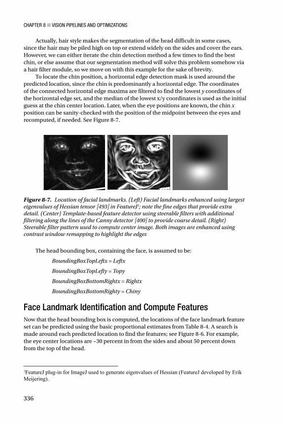
To locate the chin position, a horizontal edge detection mask is used around the predicted location, since the chin is predominantly a horizontal edge. The coordinates of the connected horizontal edge maxima are filtered to find the lowest y coordinates of the horizontal edge set, and the median of the lowest x/y coordinates is used as the initial guess at the chin center location. Later, when the eye positions are known, the chin x position can be sanity-checked with the position of the midpoint between the eyes and recomputed, if needed. See Figure 8-7 .
Figure 8-7. Location of facial landmarks . (Left) Facial landmarks enhanced using largest eigenvalues of Hessian tensor [493] in FeatureJ 1 ; note the fine edges that provide extra detail. (Center) Template-based feature detector using steerable filters with additional filtering along the lines of the Canny detector [400] to provide coarse detail. (Right) Steerable filter pattern used to compute center image. Both images are enhanced using contrast window remapping to highlight the edges
1 FeatureJ plug-in for ImageJ used to generate eigenvalues of Hessian (FeatureJ developed by Erik Meijering).
The head bounding box, containing the face, is assumed to be:
BoundingBoxTopLeftx = Leftx
BoundingBoxTopLefty = Topy
BoundingBoxBottomRightx = Rightx
BoundingBoxBottomRighty = Chiny
Face Landmark Identification and Compute Features Now that the head bounding box is computed, the locations of the face landmark feature set can be predicted using the basic proportional estimates from Table 8-4 . A search is made around each predicted location to find the features; see Figure 8-6 . For example, the eye center locations are ~30 percent in from the sides and about 50 percent down from the top of the head.

CHAPTER 8 ■ VISION PIPELINES AND OPTIMIZATIONS
337
In our system we use an image pyramid with two levels for feature searching, a coarse-level search down-sampled by four times, and a fine-level search at full resolution to relocate the interest points, compute the feature descriptors, and take the measurements. The coarse-to-fine approach allows for wide variation in the relative size of the head to account for mild scale invariance owing to distance from the camera and/or differences in head size owing to age.
We do not add a step here to rotate the head orthogonal to the Cartesian coordinates in case the head is tilted; however, this could be done easily. For example, an iterative procedure can be used to minimize the width of the orthogonal bounding box, using several rotations of the image taken every 2 degrees from -10 to +10 degrees. The bounding box is computed for each rotation, and the smallest bounding box width is taken to find the angle used to correct the image for head tilt.
In addition, we do not add a step here to compute the surface texture of the skin, useful for age detection to find wrinkles, which is easily accomplished by segmenting several skin regions, such as forehead, eye corners, and the region around mouth, and computing the surface texture (wrinkles) using an edge or texture metric.
The landmark detection steps include feature detection, feature description, and computing relative measurements of the positions and angles between landmarks, as follows:
1. Compute interest points: Prior to searching for the facial features, interest point detectors are used to compute likely candidate positions around predicted locations. Here we use a combination of two detectors: (1) the largest eigenvalue of the Hessian tensor [493], and (2) steerable filters [388] processed with an edge detection filter criteria similar to the Canny method [400], as illustrated in Figure 8-7 . Both the Hessian and the Canny-like edge detectors images are followed by contrast windowing to enhance the edge detail. The Hessian style and Canny-style images are used together to vote on the actual location of best interest points during the correlation stage next.
2. Compute landmark positions using correlation: The final position of each facial landmark feature is determined using a canonical set of correlation templates, described earlier, including eye corners, eyebrow corners, eyebrow peaks, nose corners, nose bottom, lip corners, and lip center region shapes. The predicted location to start the correlation search is the average position of both detectors from step 1: (1) The Hessian approach provides fine-feature details, (2) while the steerable filter approach provides coarse-feature details. Testing will determine if correlation alone is sufficient without needing interest points from step 1.
3. Describe landmarks using FREAK descriptors: For each landmark location found in step 2, we compute a FREAK descriptor. SIFT may work just as well.
CHAPTER 8 ■ VISION PIPELINES AND OPTIMIZATIONS
338
4. Measure dominant eye color using CIECAM02 JCH: We use a super-pixel method [257,258] to segment out the regions of color around the center of the eye, and make a histogram of the colors of the super-pixel cells. The black pupil and the white of the eye should cluster as peaks in the histogram, and the dominant color of the eye should cluster in the histogram also. Even multi-colored eyes will be recognized using our approach using histogram correspondence.
5. Compute relative positions and angles between landmarks: In step 2 above, correlation was used to find the location of each feature (to sub-pixel accuracy if desired [468]). As illustrated in Figure 8-6 , we use the landmark positions as the basis for measuring the relative distances of several features, such as:
a. Eye distance, center to center, useful for age and gender
b. Eye size, corner to corner
c. Eyebrow angle, end to center, useful for emotion
d. Eyebrow to eye angle, ends to center positions, useful for emotion
e. Eyebrow distance to eye center, useful for emotion
f. Lip or mouth width
g. Center lip ridges angle with lip corners, useful for emotion
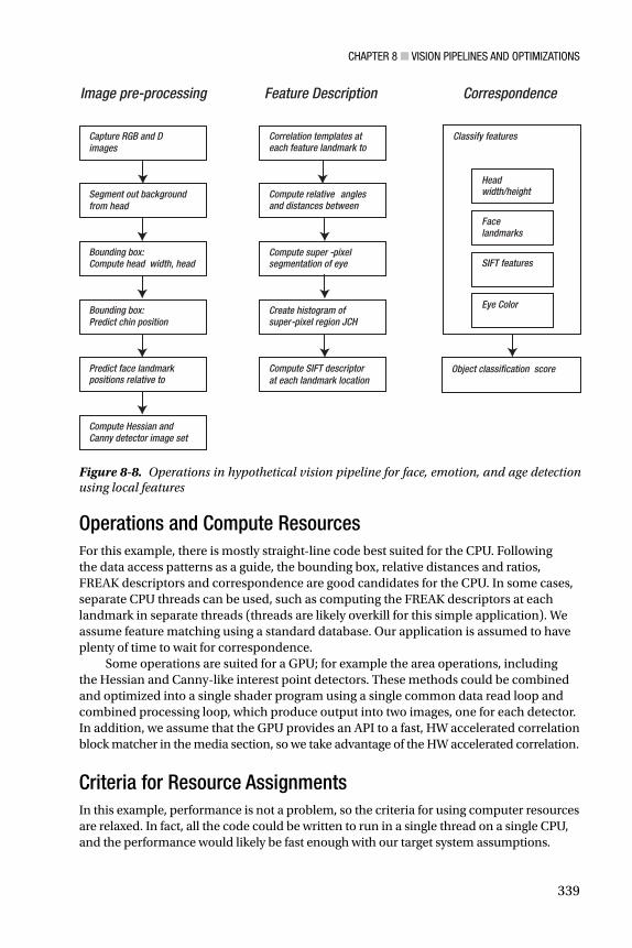
Pipeline Stages and Operations The pipeline stages and operations are shown in Figure 8-8 . For correspondence, we assume a separate database table for each feature. We are not interested in creating an optimized classifier to speed up pattern matching; brute-force searching is fine.
CHAPTER 8 ■ VISION PIPELINES AND OPTIMIZATIONS
339
Capture RGB and D images
Segment out background from head
Bounding box:Compute head width, head
Predict face landmark positions relative to
Compute Hessian and Canny detector image set
Bounding box:Predict chin position
Correlation templates at each feature landmark to
Compute relative angles and distances between
Compute super -pixel segmentation of eye
Create histogram of super-pixel region JCH
Compute SIFT descriptor at each landmark location
Classify features
Head width/height
Eye Color
Face landmarks
SIFT features
Object classification score
Image pre-processing Feature Description Correspondence
Figure 8-8. Operations in hypothetical vision pipeline for face, emotion, and age detection using local features
Operations and Compute Resources For this example, there is mostly straight-line code best suited for the CPU. Following the data access patterns as a guide, the bounding box, relative distances and ratios, FREAK descriptors and correspondence are good candidates for the CPU. In some cases, separate CPU threads can be used, such as computing the FREAK descriptors at each landmark in separate threads (threads are likely overkill for this simple application). We assume feature matching using a standard database. Our application is assumed to have plenty of time to wait for correspondence.
Some operations are suited for a GPU; for example the area operations, including the Hessian and Canny-like interest point detectors. These methods could be combined and optimized into a single shader program using a single common data read loop and combined processing loop, which produce output into two images, one for each detector. In addition, we assume that the GPU provides an API to a fast, HW accelerated correlation block matcher in the media section, so we take advantage of the HW accelerated correlation.
Criteria for Resource Assignments In this example, performance is not a problem, so the criteria for using computer resources are relaxed. In fact, all the code could be written to run in a single thread on a single CPU, and the performance would likely be fast enough with our target system assumptions.
CHAPTER 8 ■ VISION PIPELINES AND OPTIMIZATIONS
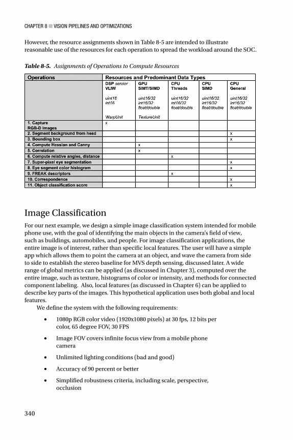
340
However, the resource assignments shown in Table 8-5 are intended to illustrate reasonable use of the resources for each operation to spread the workload around the SOC.
Table 8-5. Assignments of Operations to Compute Resources
Image Classification For our next example, we design a simple image classification system intended for mobile phone use, with the goal of identifying the main objects in the camera’s field of view, such as buildings, automobiles, and people. For image classification applications, the entire image is of interest, rather than specific local features. The user will have a simple app which allows them to point the camera at an object, and wave the camera from side to side to establish the stereo baseline for MVS depth sensing, discussed later. A wide range of global metrics can be applied (as discussed in Chapter 3), computed over the entire image, such as texture, histograms of color or intensity, and methods for connected component labeling. Also, local features (as discussed in Chapter 6) can be applied to describe key parts of the images. This hypothetical application uses both global and local features.
We define the system with the following requirements :
1080p RGB color video (1920x1080 pixels) at 30 fps, 12 bits per • color, 65 degree FOV, 30 FPS
Image FOV covers infinite focus view from a mobile phone • camera
Unlimited lighting conditions (bad and good) •
Accuracy of 90 percent or better •
Simplified robustness criteria, including scale, perspective, • occlusion

CHAPTER 8 ■ VISION PIPELINES AND OPTIMIZATIONS
341
• For each image, the system computes the following features:
• Global RGBI histogram, in RGB-I color space
• GPS coordinates, since the phone has a GPS
• Camera pose via MVS depth sensing, using the accelerometer data for geometric rectification to an orthogonal FOV plane (the user is asked to wave the camera while pointed at the subject, the camera pose vector is computed from the accelerometer data and relative to the main objects in the FOV using ICP)
• SIFT features, ideally between 20 and 30 features stored for each image
• Depth map via monocular dense depth sensing, used to segment out objects in the FOV, depth range target 0.3 meters to 30 meters, accuracy within 1 percent at 1 meter, and within 10 percent at 30 meters
• Scene labeling and pixel labeling, based on attributes of segmented regions, including RGB-I color and LBP texture
Scene recognition is a well-researched field, and several grand challenge competitions are held annually to find methods for increased accuracy using established ground truth datasets, as shown in Appendix B. The best accuracy achieved for various categories of images in the challenges ranges from 50 to over 90 percent. In this exercise, no attempt is made to prove performance or accuracy.
Segmenting Images and Feature Descriptors For this hypothetical vision pipeline, several methods for segmenting the scene into objects will be used together, instead of relying on a single method, as follows:
1. Dense segmentation, scene parsing, and object labeling: A depth map generated using monocular MVS is used to segment common items in the scene, including the ground or floor, sky or ceiling, left and right walls, background, and subjects in the scene. To compute monocular depth from the mobile phone device, the user is prompted by the application to move the camera from left to right over a range of arm’s length covering 3 feet or so, to create a series of wide baseline stereo images for computing depth using MVS methods (as discussed in Chapter 1). MVS provides a dense depth map. Even though MVS computation is compute-intensive, this is not a problem, since our application does not require continuous real-time depth map generation – just a single depth map; 3 to 4 seconds to acquire the baseline images and generate the depth map is assumed possible for our hypothetical mobile device.

CHAPTER 8 ■ VISION PIPELINES AND OPTIMIZATIONS
342
2. Color segmentation and component labeling using super-pixels: The color segmentation using super-pixels should correspond roughly with portions of the depth segmentation.
3. LBP region segmentation: This method is fairly fast to compute and compact to represent, as discussed in Chapter 6.
4. Fused segmentation: The depth, color, and LBP segmentation regions are combined using Boolean masks and morphology and some logic into a fused segmentation. The method uses an iterative loop to minimize the differences between color, depth, and LBP segmentation methods into a new fused segmentation map. The fused segmentation map is one of the global image descriptors.
5. Shape features for each segmented region: basic shape features, such as area and centroid, are computed for each fused segmentation region. Relative distance and angle between region centroids is also computed into a composite descriptor.
In this hypothetical example, we use several feature descriptor methods together for additional robustness and invariance, and some pre-processing, summarized as follows:
1. SIFT interest points across the entire image are used as additional clues. We follow the SIFT method exactly, since SIFT is known to recognize larger objects using as few as three or four SIFT features [161]. However, we expect to limit the SIFT feature count to 20 or 30 strong candidate features per scene, based on training results.
2. In addition, since we have an accelerometer and GPS sensor data on the mobile phone, we can use sensor data as hints for identifying objects based on location and camera pose alone, for example assuming a server exists to look up the GPS coordinates of landmarks in an area.
3. Since illumination invariance is required, we perform RGBI contrast remapping in an attempt to normalize contrast and color prior to the SIFT feature computations, color histograms, and LBP computations. We assume a statistical method for computing the best intensity remapping limits is used to spread out the total range of color to mitigate dark and oversaturated images, based on ground truth data testing, but we do not take time to develop the algorithm here; however, some discussion on candidate algorithms is provided in Chapter 2. For example, computing SIFT descriptors on dark images may not provide sufficient edge gradient information to compute a good SIFT descriptor, since SIFT requires gradients. Oversaturated images will have washed-out color, preventing good color histograms.

CHAPTER 8 ■ VISION PIPELINES AND OPTIMIZATIONS
343
4. The fused segmentation combines the best of all the color, LBP, and depth segmentation methods, minimizing the segmentation differences by fusing all segmentations into a fused segmentation map. LBP is used also, which is less sensitive to both low light and oversaturated conditions, providing some balance.
Again, in the spirit of a hypothetical exercise, we do not take time here to develop the algorithm beyond the basic descriptions given above.
Pipeline Stages and Operations The pipeline stages are shown in Figure 8-9 . They include an image pre-processing stage primarily to correct image contrast, compute depth maps and segmentation maps. The feature description stage computes the RGBI color histograms, SIFT features, a fused segmentation map combining the best of depth, color, and LBP methods, and then labels the pixels as connected components. For correspondence, we assume a separate database table for each feature, using brute-force search; no optimization attempted.
Capture wide baseline images
RGBI contrast remapping
Compute MVS depth map
Color segmentation map
LBP texture segmentation map
Compute RGBI color histograms
Compute SIFT features
Compute fused -segmentation
Labeling segmented objects
Classify features
Histograms
GPS, camera pose
Segmented Objects
SIFT features
Object classification score
Image pre-processing Feature Description Correspondence
Figure 8-9. Operations in hypothetical image classification pipeline using global features
Mapping Operations to Resources We assume that the DSP provides an API for contrast remapping, and since the DSP is already processing all the pixels from the sensor anyway and the pixel data is already there, contrast remapping is a good match for the DSP.
The MVS depth map computations follow a data pattern of line and area operations. We use the GPU for the heavy-lifting portions of the MVS algorithm, like left/right image

CHAPTER 8 ■ VISION PIPELINES AND OPTIMIZATIONS
344
pair pattern matching. Our algorithm follows the basic stereo algorithms, as discussed in Chapter 1. The stereo baseline is estimated initially from the accelerometer, then some bundle adjustment iterations over the baseline image set are used to improve the baseline estimates. We assume that the MVS stereo workload is the heaviest in this pipeline and consumes most of the GPU for a second or two. A dense depth map is produced in the end to use for depth segmentation.
The color segmentation is performed on RGBI components using a super-pixel method [257,258]. A histogram of the color components is also computed in RGBI for each superpixel cell. The LBP texture computation is a good match for the GPU since it is an area operation amenable to shader programming style. So, it is possible to combine the color segmentation and the LBP texture segmentation into the same shader to leverage data sharing in register files and avoid data swapping and data copies.
The SIFT feature description can be assigned to CPU threads , and the data can be tiled and divided among the CPU threads for parallel feature description. Likewise, the fused segmentation can be assigned to CPU threads and the data tiled also. Note that tiled data can include overlapping boundary regions or buffers, see later Figure 8-12 for an illustration of overlapped data tiling. Labeling can also be assigned to parallel CPU threads in a similar manner, using tiled data regions. Finally, we assume a brute-force matching stage using database tables for each descriptor to develop the final score, and we weight some features more than others in the final scoring, based on training against ground truth data.
Criteria for Resource Assignments The basic criterion for the resource assignments is to perform the early point processing on the DSP, since the data is already resident, and then to use the GPU SIMT SIMD model to compute the area operations as shaders to create the depth maps, color segmentation maps, and LBP texture maps. The last stages of the pipeline map nicely to thread parallel methods and data tiling. Given the chosen operation to resource assignments shown in Table 8-6 , this application seems cleanly amenable to workload balancing and parallelization across the CPU cores in threads and the GPU.
Table 8-6. Assignments of Operations to Compute Resources
CHAPTER 8 ■ VISION PIPELINES AND OPTIMIZATIONS
345
Augmented Reality In this fourth example, we design an augmented reality application for equipment maintenance using a wearable display device such as glasses or goggles and wearable cameras. The complete system consists of a portable, wearable device with camera and display connected to a server via wireless. Processing is distributed between the wearable device and the server. ( Note: this example is especially high level and leaves out a lot of detail, since the actual system would be complex to design, train and test.)
The server system contains all the CAD models of the machine and provides on-demand graphics models or renderings of any machine part from any viewpoint. The wearable cameras track the eye gaze and the position of the machine. The wearable display allows a service technician to look at a machine and view augmented reality overlays on the display, illustrating how to service the machine. As the user looks at a given machine, the augmented reality features identify the machine parts and provide overlays and animations for assisting in troubleshooting and repair. The system uses a combination of RGB images as textures on 3D depth surfaces and a database of 3D CAD models of the machine and all the component machine parts.
The system will have the following requirements :
1080p RGB color video camera (1920x1080 pixels) at 30 fps, 12 bits • per color, 65 degree FOV, 30 FPS
1080p stereo depth camera with 8 bits Z resolution at 60 fps, • 65 degree FOV; all stereo processing performed in silicon in the camera ASIC with a depth map as output
480p near infra-red camera pointed at eyes of technician, used for • gaze detection; the near-infrared camera images better in the low-light environment around the head-mounted display
1080p wearable RGB display •
A wearable PC to drive the cameras and display, descriptor • generation, and wireless communications with the server; the system is battery powered for mobile use with an 8-hour battery life
A server to contain the CAD models of the machines and parts; • each part will have associated descriptors pre-computed into the data base; the server can provide either graphics models or complete renderings to the wearable device via wireless
Server to contain ground truth data consisting of feature • descriptors computed on CAD model renderings of each part + normalized 3D coordinates for each descriptor for machine parts
Simplified robustness criteria include perspective, scale, and • rotation
CHAPTER 8 ■ VISION PIPELINES AND OPTIMIZATIONS
346
Calibration and Ground Truth Data We assume that the RGB camera and the stereo camera system are calibrated with correct optics to precisely image the same FOV, since the RGB camera and 3D depth map must correspond at each pixel location to enable 2D features to be accurately associated with the corresponding 3D depth location. However, the eye gaze camera will require some independent calibration, and we assume a simple calibration application is developed to learn the technician’s eye positions by using the stereo and RGB cameras to locate a feature in the FOV, and then overlay an eye gaze vector on a monitor to confirm the eye gaze vector accuracy. We do not develop the calibration process here.
However, the ground truth data takes some time to develop and train, and requires experts in repair and design of the machine to work together during training. The ground truth data includes feature sets for each part, consisting of 2D SIFT features along corners, edges, and other locations such as knobs. To create the SIFT features, first a set of graphics renderings of each CAD part model is made from representative viewpoints the technician is likely to see, and then the 2D SIFT features are computed on the graphics renderings, and the geometry of the model is used to create relative 3D coordinates for each SIFT feature for correspondence.
The 2D SIFT feature locations are recorded in the database along with relative 3D coordinates, and associated into objects using suitable constraints such as angles and relative distances, see Figure 8-10 . An expert selects a minimum set of features for each part during training—primarily strongest features from corners and edges of surfaces. The relative angles and distances in three dimensions between the 2D SIFT features are recorded in the database to provide for perspective, scale, and rotation invariance. The 3D coordinates for all the parts are normalized to the size of the machine. In addition, the dominant color and texture of each part surface is computed from the renderings and stored as texture and color features. This system would require considerable training and testing.
Feature and Object Description In actual use in the field, the RGB camera is used to find the 2D SIFT, LBP and color features, and the stereo camera is used to create the depth map. Since the RGB image and depth map are pixel-aligned, each feature has 3D coordinates taken from the depth map, which means that a 3D coordinate can be assigned to a 2D SIFT feature location. The 3D angles and 3D distances between 2D SIFT feature locations are computed as constraints, and the combined LBP, color and 2D SIFT features with 3D location constraints are stored as SIFT vertex features and sent to the server for correspondence. See Figure 8-10 for an illustration of the layout of the SIFT vertex descriptors and parts objects. Note that the 3D coordinate is associated with several descriptors, including SIFT, LBP texture, ands RGB color, similar to the way a 3D vertex is represented in computer graphics by 3D location, color, and texture. During training, several SIFT vertex descriptors are created from various views of the parts, each view associated by 3D coordinates in the database, allowing for simplified searching and matching based on 3D coordinates along with the features.
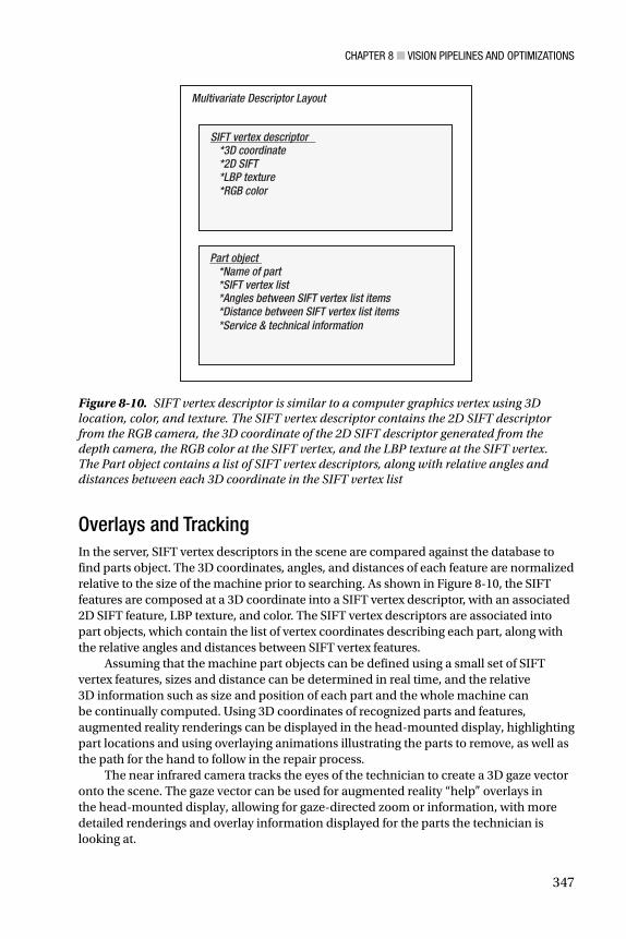
CHAPTER 8 ■ VISION PIPELINES AND OPTIMIZATIONS
347
Overlays and Tracking In the server, SIFT vertex descriptors in the scene are compared against the database to find parts object. The 3D coordinates, angles, and distances of each feature are normalized relative to the size of the machine prior to searching. As shown in Figure 8-10 , the SIFT features are composed at a 3D coordinate into a SIFT vertex descriptor, with an associated 2D SIFT feature, LBP texture, and color. The SIFT vertex descriptors are associated into part objects, which contain the list of vertex coordinates describing each part, along with the relative angles and distances between SIFT vertex features.
Assuming that the machine part objects can be defined using a small set of SIFT vertex features, sizes and distance can be determined in real time, and the relative 3D information such as size and position of each part and the whole machine can be continually computed. Using 3D coordinates of recognized parts and features, augmented reality renderings can be displayed in the head-mounted display, highlighting part locations and using overlaying animations illustrating the parts to remove, as well as the path for the hand to follow in the repair process.
The near infrared camera tracks the eyes of the technician to create a 3D gaze vector onto the scene. The gaze vector can be used for augmented reality “help” overlays in the head-mounted display, allowing for gaze-directed zoom or information, with more detailed renderings and overlay information displayed for the parts the technician is looking at.
Multivariate Descriptor Layout
SIFT vertex descriptor*3D coordinate*2D SIFT*LBP texture*RGB color
Part object*Name of part *SIFT vertex list*Angles between SIFT vertex list items*Distance between SIFT vertex list items*Service & technical information
Figure 8-10. SIFT vertex descriptor is similar to a computer graphics vertex using 3D location, color, and texture. The SIFT vertex descriptor contains the 2D SIFT descriptor from the RGB camera, the 3D coordinate of the 2D SIFT descriptor generated from the depth camera, the RGB color at the SIFT vertex, and the LBP texture at the SIFT vertex. The Part object contains a list of SIFT vertex descriptors, along with relative angles and distances between each 3D coordinate in the SIFT vertex list

CHAPTER 8 ■ VISION PIPELINES AND OPTIMIZATIONS
348
Pipeline Stages and Operations The pipeline stages are shown in Figure 8-11 . Note that the processing is divided between the wearable device (primarily for image capture, feature description, and display), and a server for heavy workloads, such as correspondence and augmented reality renderings. In this example, the wearable device is used in combination with the server, relying on a wireless network to transfer images and data. We assume that data bandwidth and data compression methods are adequate on the wireless network for all necessary data communications.
Figure 8-11. Operations in hypothetical augmented reailty pipeline
Mapping Operations to Resources We make minimal use of the GPU for GPGPU processing and assume the server has many CPUs available, and we use the GPU for graphics rendering at the end of the pipeline. Most of the operations map well into separate CPU threads using data tiling. Note that a server commonly has many high-power and fast CPUs, so using CPU threads is a good match. See Table 8-7 .

CHAPTER 8 ■ VISION PIPELINES AND OPTIMIZATIONS
349
Criteria for Resource Assignments On the mobile device, the depth map is computed in silicon on the depth camera. We use the GPU to perform the RGB and depth map alignment using the texture sampler, then perform SIFT computations on the CPU, since the SIFT computations must be done first to have the vertex to anchor and compute the multivariate descriptor information. We continue and follow data locality and perform the LBP and color computations for each 2D SIFT point in separate CPU threads using data tiling and overlapped regions. See later Figure 8-12 for an illustration of overlapped data tiling.
Table 8-7. Assignments of Operations to Compute Resources
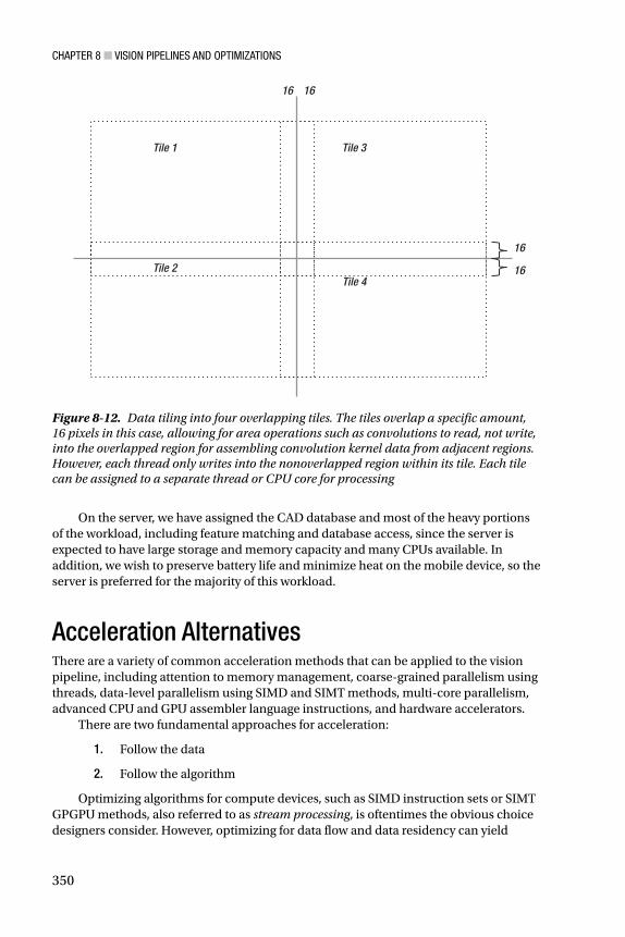
CHAPTER 8 ■ VISION PIPELINES AND OPTIMIZATIONS
350
On the server, we have assigned the CAD database and most of the heavy portions of the workload, including feature matching and database access, since the server is expected to have large storage and memory capacity and many CPUs available. In addition, we wish to preserve battery life and minimize heat on the mobile device, so the server is preferred for the majority of this workload.
Acceleration Alternatives There are a variety of common acceleration methods that can be applied to the vision pipeline, including attention to memory management, coarse-grained parallelism using threads, data-level parallelism using SIMD and SIMT methods, multi-core parallelism, advanced CPU and GPU assembler language instructions, and hardware accelerators.
There are two fundamental approaches for acceleration:
1. Follow the data
2. Follow the algorithm
Optimizing algorithms for compute devices, such as SIMD instruction sets or SIMT GPGPU methods, also referred to as stream processing , is oftentimes the obvious choice designers consider. However, optimizing for data flow and data residency can yield
Tile 1
Tile 2
Tile 3
Tile 4
16
16
16 16
Figure 8-12. Data tiling into four overlapping tiles. The tiles overlap a specific amount, 16 pixels in this case, allowing for area operations such as convolutions to read, not write, into the overlapped region for assembling convolution kernel data from adjacent regions. However, each thread only writes into the nonoverlapped region within its tile. Each tile can be assigned to a separate thread or CPU core for processing
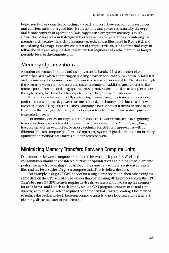
CHAPTER 8 ■ VISION PIPELINES AND OPTIMIZATIONS
351
better results. For example, bouncing data back and forth between compute resources and data formats is not a good idea; it eats up time and power consumed by the copy and format conversion operations. Data copying in slow-system memory is much slower than data access in fast-register files within the compute units. Considering the memory architecture hierarchy of memory speeds, as was illustrated in Figure 8-2 , and considering the image-intensive character of computer vision, it is better to find ways to follow the data and keep the data resident in fast registers and cache memory as long as possible, local to the compute unit.
Memory Optimizations Attention to memory footprint and memory transfer bandwidth are the most often overlooked areas when optimizing an imaging or vision application. As shown in Table 8-2 and the memory discussion following, a vision pipeline moves several GB/S of data through the system between compute units and system memory. In addition, area processes like interest point detection and image pre-processing move even more data in complex routes through the register files of each compute unit, caches, and system memory.
Why optimize for memory? By optimizing memory use, data transfers are reduced, performance is improved, power costs are reduced, and battery life is increased. Power is costly; in fact, a large Internet search company has built server farms very close to the Columbia River’s hydroelectric systems to guarantee clean power and reduce power transmission costs.
For mobile devices, battery life is a top concern. Governments are also beginning to issue carbon taxes and credits to encourage power reductions. Memory use, thus, is a cost that’s often overlooked. Memory optimization APIs and approaches will be different for each compute platform and operating system. A good discussion on memory optimization methods for Linux is found in reference[494].
Minimizing Memory Transfers Between Compute Units Data transfers between compute units should be avoided, if possible. Workload consolidation should be considered during the optimization and tuning stage in order to perform as much processing as possible on the same data while it is resident in register files and the local cache of a given compute unit. That is, follow the data.
For example, using a GPGPU shader for a single-area operation, then processing the same data on the CPU will likely be slower than performing all the processing on the CPU. That’s because GPGPU kernels require device driver intervention to set up the memory for each kernel and launch each kernel, while a CPU program accesses code and data directly, with no driver set-up required other than initial program loading. One method to reduce the back-and-forth between compute units is to use loop coalescing and task chaining, discussed later in this section.

CHAPTER 8 ■ VISION PIPELINES AND OPTIMIZATIONS
352
Memory Tiling When dividing workloads for coarse-grained parallelism into several threads, the image can be broken into tiled regions and each tile assigned to a thread. Tiling works well for point, line, and area processing, where each thread performs the same operation on the tiled region. By allowing for an overlapped read regions between tiles, the hard boundaries are eliminated and area operations like convolution can read into adjacent tiles for kernel processing, as well as write finished results into their tile.
DMA, Data Copy, and Conversions Often, multiple copies of an image are needed in the vision pipeline, and in some cases, the data must be converted from one type to another. Converting 12-bit unsigned color channel data stored in a 16-bit integer to a 32-bit integer allowing for more accurate numerical precision downstream in computations is one example. Also, the color channels might be converted into a chosen color space, such as RGBI, for color processing in the I component space (R*G*B)/3 = I; then, the new I value is mixed and copied back into the RGB components. Careful attention to data layout and data residency will allow more efficient forward and backward color conversions.
When copying data, it is good to try using the direct memory access (DMA) unit for the fastest possible data copies. The DMA unit is implemented in hardware to directly optimize and control the I/O interconnect traffic in and out of memory. Operating systems provide APIs to access the DMA unit [494]. There are variations for optimizing the DMA methods, and some interesting reading comparing cache performance against DMA in vision applications are found in references[497,495].
Register Files, Memory Caching, and Pinning The memory system is a hierarchy of virtual and physical memories for each processor, composed of slow fixed storage such as file systems, page files, and swap files for managing virtual memory, system memory, caches, and fast-register files inside compute units, and with memory interconnects in between. If the data to process is resident in the register files, it is processed by the ALU at processor clock rates. Best-case memory access is via the register files close to each ALU, so keeping the data in registers and performing all possible processing before copying the data is optimal, but this may require some code changes (discussed later in this section).
If the cache must be accessed to get the data, more clock cycles are burned (power is burned, performance is lost) compared to accessing the register files. And if there is a cache miss and much slower system memory must be accessed, typically many hundreds of clock cycles are required to move the memory to register files through the caches for ALU processing.
Operating systems provide APIs to lock or pin the data in memory, which usually increases the amount of data in cache, decreasing paging and swapping. (Swapping is a hidden copy operation carried out by the operating system automatically to make more room in system memory). When data is accessed often, the data will be resident in the faster cache memories, as was illustrated in Figure 8-2 .

CHAPTER 8 ■ VISION PIPELINES AND OPTIMIZATIONS
353
Data Structures, Packing, and Vector vs. Scatter-Gather Data Organization The data structures used contribute to memory traffic. Data organization should allow serial access in contiguous blocks as much as possible to provide best performance. From the programming perspective, data structures are often designed with convenience in mind, and no attention is given to how the compiler will arrange the data or the resulting performance.
For example, consider a data structure with several fields composed of bytes, integers, and floating point data items; compilers may attempt to rearrange the positions of data items in the data structures, and even pack the data in a different order for various optimizations. Compilers usually provide a set of compiler directives, such as in-line pragmas and compiler switches, to control the data packing behavior; these are worth looking into.
For point processing, vectors of data are the natural structure, and the memory system will operate at peak performance in accessing and processing contiguous vectors. For area operations, rectangles spanning several lines are used, and the rectangles cause memory access patterns that can generate cache misses. Using scatter-gather operations for gathering convolution kernel data allows a large data structure to be split apart into vectors of data, increasing performance. Often, CPU and GPU memory architectures pay special attention to data-access patterns and provide hidden methods for optimizations.
Scatter-gather operations, also referred to as vectored I/O or strided memory access, can be implemented in the GPU or CPU silicon to allow for rapid read/write access to noncontiguous data structure patterns. Typically, a scatter operation writes multiple input buffers into a contiguous pattern in a single output buffer, and a gather operation analogously reads multiple input buffers into a contiguous pattern in the output buffer.
Operating systems and compute languages provide APIs for scatter-gather operations. For Linux-style operating systems, see the readv and writev function specified in the POSIX 1003.1-2001 specification. The async_work_group_strided_copy function is provided by OpenCL for scatter-gather.
Coarse-Grain Parallelism A vision pipeline can be implemented using coarse-grain parallelism by breaking up the work into threads, and also by assigning work to multiple processor cores. Coarse-grained parallelism can be achieved by breaking up the compute workload into pipelines of threads, or by breaking up the memory into tiles assigned to multiple threads.
Compute-Centric vs. Data-Centric Coarse-grain parallelism can be employed via compute-centric and data-centric approaches. For example, in a compute-centric approach, vision pipeline stages can be split among independent execution threads and compute units along the lines of pipeline stages, and data is fed into the next stage a little at a time via queues and FIFOs. In a data-centric approach, an image can be split into tiles, as was shown in Figure 8-12 , and each thread processes an independent tile region.

CHAPTER 8 ■ VISION PIPELINES AND OPTIMIZATIONS
354
Threads and Multiple Cores Several methods exist to spread threads across multiple CPU cores, including reliance on the operating system scheduler to make optimum use of each CPU core and perform load balancing. Another is by assigning specific tasks to specific CPU cores. Each operating system has different controls available to tune the process scheduler for each thread, and also may provide the capability to assign specific threads to specific processors. (We discuss programming resources, languages and tools for coarse-grained threading later in this chapter.) Each operating system will provide an API for threading, such as pthreads . See Figure 8-13 .
0
5
10
15
20
25
30
35
40
GaussianPyramid
n30%
DoG 7% Scale SpaceExtrema
14%
FeatureOrientation
7%
ComputeDescriptor
36%
0
1000
2000
3000
4000
5000
6000
ORB(15.3ms)
SURF(217.3ms)
SIFT(5228.7ms)
Figure 8-13. (Left) Typical SIFT descriptor pipeline compute allocation [180]. (Right) Reported compute times [120] for ORB, SURF, and SIFT, averaged over twenty-four 640x480 images containing about 1,000 features per image. Retrofitting ORB for SIFT may be a good choice in some applications
Fine-Grain Data Parallelism Fine-grain parallelism refers to the data organization and the corresponding processor architectures exploiting parallelism, traditionally referred to as array processors or vector processors . Not all applications are data parallel. Deploying non-data-parallel code to run on a data-parallel machine is counterproductive; it’s better to use the CPU and straight-line code to start.
A data-parallel operation should exhibit common memory patterns, such as large arrays of regular data like lines of pixels or tiles of pixels, which are processed in the same way. Referring back to Figure 8-1 , note that some algorithms operate on vectors of points, lines, and pixel regions. These data patterns and corresponding processing operations are inherently data-parallel. Examples of point operations are color corrections and data-type conversions, and examples of area operations are convolution and morphology. Some algorithms are straight-line code, with lots of branching and little parallelism. Fine-grained data parallelism is supported directly via SIMD and SIMT methods.

CHAPTER 8 ■ VISION PIPELINES AND OPTIMIZATIONS
355
SIMD, SIMT, and SPMD Fundamentals The supercomputers of yesterday are now equivalent to the GPUs and multi-core CPUs of today. The performance of SIMD, SIMT, and SPMD machines, and their parallel programming languages, is of great interest to the scientific community. It has been developed over decades, and many good resources are available that can be applied to inexpensive SOCs today; see the National Center for Supercomputing Applications[544] for a starting point.
SIMD instructions and multiple threads can be applied when fine-grained parallelism exists in the data layout in memory and the algorithm itself, such as with point, line, and area operations on vectors. Single Instruction Multiple Data (SIMD) instructions process several data items in a vector simultaneously. To exploit fine-grained parallelism at the SIMD level, both the computer language and the corresponding ALUs should provide direct support for a rich set of vector data types and vector instructions. Vector-oriented programming languages are required to exploit data-parallelism, as shown in Table 8-8 ; however, sometimes compiler switches are available to exploit SIMD. Note that languages like C++ do not directly support vector data types and vector instructions, while data-parallel languages do, as shown in Table 8-8 .
Table 8-8. Common Data-Parallel Language Choices
Language Name Standard or Proprietary OS Platform Support
Pixel Shader GLSL Standard OpenGL Several OS platforms
Pixel Shader HLSL Direct3D Microsoft OS
Compute Shader Direct3D Microsoft OS
Compute Shader Standard OpenGL Several OS platforms
RenderScript Android Google OS
OpenCL Standard Several OS platforms
C++ AMP Microsoft Microsoft OS platforms
CUDA Only for NVIDIA GPUs Several OS platforms
OpenMP Standard Several OS platforms
In some cases, the cost of SIMT outweighs its benefit, especially considering run-time overhead for data set-up and tear-down, thread management, code portability problems, and scalability across large and small CPUs and GPUs.
In addition to SIMD instructions, a method for launching and managing large groups of threads running the same identical code must be provided to exploit data-parallelism, referred to as Single Instruction Multiple Threading (SIMT) , also known as Single Program Multiple Data (SPMD) . The SIMT programs are referred to as shaders , since historically the pixel shaders and vertex shaders used in computer graphics were the first programs widely used to exploit fine-grained data parallelism. Shaders are also referred to as kernels .

CHAPTER 8 ■ VISION PIPELINES AND OPTIMIZATIONS
356
Both CPUs and GPUs support SIMD instructions and SIMT methods—for example, using languages like OpenCL. The CPU uses the operating system scheduler for managing threads; however, GPUs use hardware schedulers, dispatchers, and scoreboarding logic to track thread execution and blocking status, allowing several threads running an identical kernel on different data to share the same ALU. For the GPU, each shader runs on the ALU until it is blocked on a memory transfer, a function call, or is swapped out by the GPU shader scheduler when its time slice expires.
Note that both C++ AMP and CUDA seem to provide language environments closest to C++. The programming model and language for SIMT programming contains a run-time execution component to marshal data for each thread, launch threads, and manage communications and completion status for groups of threads. Common SIMT languages are shown in Table 8-8 .
Note that CPU and GPU execution environments differ significantly at the hardware and software level. The GPU relies on device drivers for set-up and tear-down, and fixed-function hardware scheduling, while CPUs rely on the operating system scheduler and perhaps micro-schedulers. A CPU is typically programmed in C or C++, and the program executes directly from memory and is scheduled by the operating system, while a GPU requires a shader or kernel program to be written in a SIMT SIMD-friendly language such as a compute shader or pixel shader in DirectX or OpenGL, or a GPGPU language such as CUDA or OpenCL.
Furthermore, a shader kernel must be launched via a run-time system through a device driver to the GPU, and an execution context is created within the GPU prior to execution. A GPU may also use a dedicated system memory partition where the data must reside, and in some cases the GPU will also provide a dedicated fast-memory unit.
GPGPU programming has both memory data set-up and program set-up overhead through the run-time system, and unless several kernels are executed sequentially in the GPU to hide the overhead, the set-up and tear-down overhead for a single kernel can exceed any benefit gained via the GPU SIMD/SIMT processing.
The decision to use a data parallelism SIMT programming model affects program design and portability. The use of SIMT is not necessary, and in any case a standard programming language like C++ must be used to control the SIMT run-time environment, as well as the entire vision pipeline. However, the performance advantages of a data-parallel SIMT model are in some cases dramatically compelling and the best choice. Note, however, that GPGPU SIMT programming may actually be slower than using multiple CPU cores with SIMD instructions, coarse-grained threading, and data tiling, especially in cases where the GPU does not support enough parallel threads in hardware, which is the case for smaller GPUs.
Shader Kernel Languages and GPGPU As shown in Table 8-8 , there are several alternatives for creating SIMD SIMT data-parallel code, sometimes referred to as GPGPU or stream processing. As mentioned above, the actual GPGPU programs are known as shaders or kernels . Historically, pixel shaders and vertex shaders were developed as data-parallel languages for graphics standards like OpenGL and DirectX. However, with the advent of CUDA built exclusively for NVIDIA GPUs, the idea of a standard, general-purpose compute capability within the GPU

CHAPTER 8 ■ VISION PIPELINES AND OPTIMIZATIONS
357
emerged. The concept was received in the industry, although no killer apps existed and pixel shaders could also be used to get equivalent results. In the end, each GPGPU programming language translates into machine language anyway, so the choice of high-level GPGPU language may not be significant in many cases.
However, the choice of GPGPU language is sometimes limited for a vendor operating system. For example, major vendors such as Google, Microsoft, and Apple do not agree on the same approach for GPGPU and they provide different languages, which means that industry-wide standardization is still a work in progress and portability of shader code is elusive. Perhaps the closest to a portable standard solution is OpenCL, but compute shaders for DirectX and OpenGL are viable alternatives.
Advanced Instruction Sets and Accelerators Each processor has a set of advanced instructions for accelerating specific operations. The vendor processor and compiler documentation should be consulted for the latest information. A summary of advanced instructions is shown in Table 8-9 .
Table 8-9. Advanced Instruction Set Items
Instruction Type Description
Trancendentals GPU’s have special assembler instructions to compute common transcendental math functions for graphics rendering math operations, such as dot product, square root, cosine, and logarithms. In some cases, CPUs also have transcendental functions.
Fused instructions
Common operations such as multiply and add are often implemented in single fused MADD instruction, where both multiply and add are performed in a single clock cycle; the instruction may have three or more operands.
SIMD instructions
CPUs have SIMD instruction sets, such as the Intel SSE and Intel AVX instructions, similar SIMD for AMD processors, and NEON for ARM processors.
Advanced data types
Some instruction sets, such as for GPU’s, provide odd data types not supported by common language compilers, such as half-byte integers, 8-bit floating point numbers, and fixed-point numbers. Special data types may be supported by portions of the instruction set, but not all.
Memory access modifiers
Some processors provide strided memory access capability to support scatter-gather operations, bit-swizzling operations to allow for register contents to be moved and copied in programmable bit patterns, and permuted memory access patterns to support cross-lane patterns. Intel processors also provide MPX memory protection instructions for pointer checking.
(continued)

CHAPTER 8 ■ VISION PIPELINES AND OPTIMIZATIONS
358
Instruction Type Description
Security Cryptographic accelerators and special instructions may be provided for common ciphers such as SHA or AES ciphers; for example, INTEL AES-NI. In addition, Intel offers the INTEL SGX extensions to provide curtained memory regions to execute secure software; the curtained regions cannot be accessed by malware.
Hardware accelerators
Common accelerators include GPU texture samplers for image warping and sub-sampling, and DMA units for fast memory copies. Operating systems provide APIs to access the DMA unit [494]. Graphics programming languages such as OpenGL and DirectX provide access to the texture sampler, and GPGPU languages such as OpenCL and CUDA also provide texture sampler APIs.
APIs provided by operating system vendors may or may not use the special instructions. Compilers from each processor vendor will optimize all code to take best advantage of the advanced instructions; other compilers may or may not provide optimizations. However, each compiler will provide different flags to control optimizations, so code tuning and profiling are required. Using assembler language is the best way to get all the performance available from the advanced instruction sets.
Vision Algorithm Optimizations and Tuning Optimizations can be based on intuition or on performance profiling, usually a combination of both. Assuming that the hot spots are identified, a variety of optimization methods can be applied as discussed in this section. Performance hotspots can be addressed from the data perspective, the algorithm perspective, or both. Most of the time memory access is a hidden cost, and not understood by the developer (the algorithms are hard enough). However memory optimizations alone can be the key to increasing performance. Table 8-11 summarizes various approaches for optimizations, which are discussed next.
Data access patterns for each algorithm can be described using the Zinner, Kubinger, and Isaac taxonomy [494] shown in Table 8-10 . Note that usually the preferred data access pattern is in-place (IP) computations, which involve reading the data once into fast registers, processing and storing the results in the registers, and writing the final results back on top of the original image. This approach takes maximal advantage of the cache lines and the registers, avoiding slower memory until the data is processed.
Table 8-9. (continued)

CHAPTER 8 ■ VISION PIPELINES AND OPTIMIZATIONS
359
Compiler And Manual Optimizations Usually a good compiler can automatically perform many of the optimizations listed in Table 8-11 ; however, check the compiler flags to understand the options. The goal of the optimizations is to keep the CPU instruction execution pipelines full, or to reduce memory traffic. However, many of the optimizations in Table 8-11 require hand coding to boil down the algorithm into tighter loops with more data sharing in fast registers and less data copying.
Table 8-10. Image Processing Data Access Pattern Taxonomy (from Zinner et al.[494])
Type Description Source Images Destination Images READ WRITE
(1S) 1 source, 0 destination
1 0 Source image
no
(2S) 2 source, 0 destination
2 0 Source images
no
(IP) In-place* 1 0 Source image
Source image
(1S1D) 1 source, 1 destination
1 1 Source image
Destination image
(2S1D) 2 source, 1 destination
2 1 Source images
Destination image
*IP processing is usually the simplest way to reduce memory read/write bandwidth and memory footprint.
Table 8-11. Common Optimization Techniques, Manual And Compiler Methods
Name Description
Sub-function inlining Eliminating function calls by copying the function code in-line
Task chaining Feeding the output of a function into a waiting function piece by piece
Branch elimination Re-coding to eliminate conditional branches, or reduce branches by combining multiple branch conditions together
Loop coalescing Combining inner and outer loops into fewer loops using more straight line code
Packing data Rearranging data alignment within structures and adding padding to certain data items for better data alignment to larger data word or page boundaries to allow for more efficient memory read and write
(continued)

CHAPTER 8 ■ VISION PIPELINES AND OPTIMIZATIONS
360
Tuning After optimizing, tuning a working vision pipeline can be accomplished from several perspectives. The goal is to provide run-time controls . Table 8-12 provides some examples of tuning controls that may be implemented to allow for run-time or compile-time tuning.
Name Description
Loop unrolling Reducing the loop iteration count by replicating code inside the loop; may be accomplished using straight line code replication or by packing multiple iterations into a VLIW
Function coalescing* Rewriting serial functions into a single function, with a single outer loop to read and write data to system memory; passing small data items in fast registers between coalesced functions instead of passing large images buffers
ROS-DMA* Double-buffering DMA overlapped with processing; DMA and processing occur in parallel, DMA the new data in during processing, DMA the results out
* Function coalescing and ROS-DMA are not compiler methods, and may be performed at the source code level.
Note: See references[498,499] for more information on compiler optimizations, and see each vendor’s compiler documentation for information on available optimization controls.
Table 8-11. (continued)
Table 8-12. Run-Time Tuning Controls for a Vision Pipeline
Image Resolution Allowing variable resolution over an octave scale or other scale to reduce workload
Frames per second Skipping frames to reduce the workload
Feature database size and accuracy
Finding ways to reduce the size of the database, for example have one data base with higher accuracy, and another database with lower accuracy, each built using a different classier
Feature database organization and speed
Improving performance through better organization and searching, perhaps have more than one database, each using a different organization strategy and classifier
Feature Descriptor Retrofit, Detectors, Distance Functions As discussed in Chapter 6, many feature descriptor methods such as SIFT can be retro-fitted to use other representations and feature descriptions. For example, the LBP-SIFT retrofit discussed in Chapter 6 uses a local binary pattern in place of the gradient methods used by SIFT for impressive speedup, while preserving the other aspects of the SIFT pipeline.

CHAPTER 8 ■ VISION PIPELINES AND OPTIMIZATIONS
361
The ROOT-SIFT method is another SIFT acceleration alternative discussed in Chapter 6. Detectors and descriptors can be mixed and matched to achieve different combinations of invariance and performance, see the REIN framework [397].
In addition to the descriptor extractor itself, the distance functions often consume considerable time in the feature matching stage. For example, local binary descriptors such as FREAK and ORB use fast Hamming distance, while SIFT uses the Euclidean distance, which is slower. Retro-fitting the vision pipeline to use a local binary descriptor is an example of how the distance function can have a significant performance impact.
It should be pointed out that the descriptors reviewed in Chapter 6 are often based on academic research, not on extensive engineering field trials and optimizations. Each method is just a starting point for further development and customization. We can be sure that military weapon systems have been using similar, but far more optimal feature description methods for decades within vision pipelines in deployed systems. See Figure 8-13 .
Boxlets and Convolution Acceleration Convolution is one of the most common operations in feature description and image pre-processing, so convolution is a key target for optimizations and hardware acceleration. The boxlet method [392] approximates convolution and provides a speed vs. accuracy tradeoff. Boxlets can be used to optimize any system that relies heavily on convolutions, such as the convolutional network approach used by LeCun and others [85,336,339]. The basic approach is to approximate a pair of 2D signals, the kernel and the image, as low-degree polynomials, which quantizes each signal and reduces the data size; and then differentiating the two signals to obtain the impulse functions and convolution approximation. The full convolution can be recovered by integrating the result of the differentiation.
Another convolution and general area processing acceleration method is to reuse as much overlapping data as possible while it exists in fast registers, instead of reading the entire region of data items for each operation. When performing area operations, it is possible to program to use sliding windows and pointers in an attempt to reuse data items from adjacent rectangles that are already in the register files, rather than copying complete new rectangles into registers for each area operation. This is another area suited for silicon acceleration.
Also, scatter-gather instructions can be used to gather the convolution data into memory for accelerated processing in some cases, and GPUs often optimize the memory architecture for fast area operations.
Data-Type Optimizations, Integer vs. Float Software engineers usually use integers as the default data type , with little thought about memory and performance. Often, there is low-hanging fruit in most code in the area of data types. For example, conversion of data from int32 to int16 , and conversion from double to float , are obvious space-savings items to consider when the extra bit precision is not needed.

CHAPTER 8 ■ VISION PIPELINES AND OPTIMIZATIONS
362
In some cases, floating-point data types are used when an integer will do equally well. Floating-point computations in general require nearly four times more silicon area, which consumes correspondingly more power. The data types consume more memory and may require more clock cycles to compute. As an alternative to floating point, some processors provide fixed-point data types and instructions, which can be very efficient.
Optimization Resources Several resources in the form of software libraries and tools are available for computer vision and image processing optimizations. Some are listed in Table 8-13 .
Table 8-13. Vision Optimization Resources
Method Acceleration Strategy Examples
Threading libraries Coarse-grained parallelism Intel TBB, pthreads
Pipeline building tools
Connect functions into pipelines PfeLib Vision Pipeline Library [495]
Halide [543]*
Primitive acceleration libraries
Functions are pre-optimized Intel IPP, NVIDIA NPP, Qualcomm FastCV
GPGPU languages Develop SIMT SIMD code CUDA, OpenCL, C++ AMP, INTEL CILK++, GLSL, HLSL, Compute Shaders for OpenGL and Direct3D, RenderScript
Compiler flags Compiler optimizes for each processor; see Table 8-10
Vendor-specific
SIMD instructions Directly code in assembler, or use compiler flags for standard languages, or use GPGPU languages.
Vendor-specific
Hardware accelerators
Silicon accelerators for complex functions
Texture Samplers; others provided selectively by vendors
Advanced instruction sets
Accelerate complex low-level operations, or fuse multiple instructions; see Table 8-9
INTEL AVX, ARM NEON, GPU instruction sets
*Open source available.

CHAPTER 8 ■ VISION PIPELINES AND OPTIMIZATIONS
363
Summary This chapter ties together the discussions from previous chapters into complete vision systems by developing four purely hypothetical high-level application designs. Design details such as compute resource assignments and optimization alternatives are discussed for each pipeline, intended to generate a discussion about how to design efficient systems (the examples are sketchy at times). The applications explored include automobile recognition using shape and color features, face and emotion detection using sparse local features, whole image classification using global features, and augmented reality. Each example illustrates the use of different feature descriptor families from the Vision Metrics Taxonomy presented in Chapter 5, such as polygon shape methods, color descriptors, sparse local features, global features, and depth information. A wide range of feature description methods were used in the examples to illustrate the challenges in the pre-processing stage.
In addition, a general discussion of design concepts for optimizations and load balancing across the compute resources in the SOC fabric (CPU, GPU, and memory) was provided to explore HW/SW system challenges, such as power reductions. Finally, an overview of SW optimization resources and specific optimization techniques was presented .