Embed Size (px)
Citation preview
VISION BASED CONTROL FOR INDUSTRIAL ROBOTS
Research and implementation
Bachelor Degree Project in Automation Engineering
Bachelor Level 30 ECTS
Spring term 2019
Author: David Morilla Cabello
Supervisor: Patrik Gustavsson
Examiner: Richard Senington


ii David Morilla Cabello
School of Engineering Science 2019/06/04
Certify of authenticity
Submitted by David Morilla Cabello to the University of Skövde as a Bachelor degree
thesis at the School of Technology and Society. I certify that all material in this thesis
project which is not our own work has been identified.
Skövde, 03/06/2019
……………………………………………………………….……
Place and date
……………………………………………………………….……
Signature

iii David Morilla Cabello
School of Engineering Science 2019/06/04
Abstract
The automation revolution already helps in many tasks that are now performed by
robots. Increases in the complexity of problems regarding robot manipulators require
new approaches or alternatives in order to solve them. This project comprises a research
in different available software for implementing easy and fast visual servoing tasks
controlling a robot manipulator. It focuses on out-of-the-box solutions. Then, the tools
found are applied to implement a solution for controlling an arm from Universal Robots.
The task is to follow a moving object on a plane with the robot manipulator. The research
compares the most popular software, the state-of-the-art alternatives, especially in
computer vision and also robot control. The implementation aims to be a proof of
concept of a system divided by each functionality (computer vision, path generation and
robot control) in order to allow software modularity and exchangeability. The results
show various options for each system to take into consideration. The implementation is
successfully completed, showing the efficiency of the alternatives examined. The chosen
software is MATLAB and Simulink for computer vision and trajectory calculation
interfacing with Robotic Operating System (ROS). ROS is used for controlling a UR3 arm
using ros_control and ur_modern_driver packages. Both the research and the
implementation present a first approach for further applications and understanding over
the current technologies for visual servoing tasks. These alternatives offer different easy,
fast, and flexible methods to confront complex computer vision and robot control
problems.
iv David Morilla Cabello
School of Engineering Science 2019/06/04
Acknowledgements
First and foremost, I would like to acknowledge the support of my main supervisor Patrik
Gustavsson as well as the trust he put in me. Thank you for offering me this project
despite knowing about the difficulties it could pose. Your guidance and advice
compensated for my lack of a partner.
Furthermore, I would like to thank the University of Skövde, for allowing
international students to improve their academic and personal knowledge. The help and
attention offered by all the personnel, professors and students made me feel at home,
and all the material and facilities provided were indispensable for the accomplishment
of the project.
The help from all my colleagues and friends provided me with the support needed to
complete this venture. The teamwork and shared hours were essential in both an
academic and emotional level.
Last but not least, I would like to thank my family. Their support and education
through all these years of study made this ambitious project possible. Thanks to their
encouragement to study abroad, I was able to discover new countries, cultures and ways
of thinking.

v David Morilla Cabello
School of Engineering Science 2019/06/04
Table of contents
1 Introduction .............................................................................................................................. 1
1.1 Background ............................................................................................................................................................ 1
1.2 Problem description .............................................................................................................................................. 2
1.3 Aim and objectives ................................................................................................................................................ 2
1.3.1 Research ......................................................................................................................................................... 2
1.3.2 Implementation ............................................................................................................................................. 3
1.4 Delimitation ........................................................................................................................................................... 3
1.5 Sustainability ......................................................................................................................................................... 4
1.6 Thesis structure ..................................................................................................................................................... 5
2 Methodology ............................................................................................................................ 6
2.1 Research principles ............................................................................................................................................... 6
2.2 Research method .................................................................................................................................................. 7
3 Frame of reference ................................................................................................................ 10
3.1 Computer vision .................................................................................................................................................. 10
3.1.1 Image processing .......................................................................................................................................... 10
3.1.2 Feature detection .......................................................................................................................................... 11
3.1.3 Tracking systems ......................................................................................................................................... 12
3.1.4 Camera calibration ...................................................................................................................................... 13
3.1.5 Visual servoing ............................................................................................................................................. 14
3.2 Industrial robot ................................................................................................................................................... 15
3.2.1 Control .......................................................................................................................................................... 16
3.2.2 Kinematics of a robot manipulator ............................................................................................................. 18
3.2.3 Simulation ................................................................................................................................................... 19
4 Literature review ................................................................................................................... 20
4.1 Computer vision alternatives ............................................................................................................................. 20
4.1.1 Algorithms ................................................................................................................................................... 20
4.1.2 Software ....................................................................................................................................................... 21

vi David Morilla Cabello
School of Engineering Science 2019/06/04
4.1.3 Hardware ..................................................................................................................................................... 22
4.2 Robot control ...................................................................................................................................................... 23
5 Overall design of the system .................................................................................................. 24
6 Computer vision system ........................................................................................................ 26
6.1 Software comparison and selection .................................................................................................................... 26
6.2 System implementation ...................................................................................................................................... 29
6.2.1 MATLAB scripting and Simulink comparison ........................................................................................... 29
6.2.2 Model description ....................................................................................................................................... 29
7 Robot control ......................................................................................................................... 38
7.1 Alternatives analysis ............................................................................................................................................38
7.2 System implementation ......................................................................................................................................38
8 Robot simulation ................................................................................................................... 40
8.1 Simulation in Simulink with Simscape Multibody ........................................................................................... 40
8.2 Simulation in Gazebo.......................................................................................................................................... 44
8.3 Simulation using URSim .................................................................................................................................... 45
9 Robot interfaces .................................................................................................................... 46
9.1 Alternatives .......................................................................................................................................................... 46
9.2 UR (modern) Driver .......................................................................................................................................... 48
9.3 ros_control .......................................................................................................................................................... 49
9.4 Interface between MATLAB and ROS................................................................................................................ 51
10 Results ................................................................................................................................. 55
11 Discussion ............................................................................................................................ 60
12. Conclusion ...........................................................................................................................61
References ................................................................................................................................ 63

vii David Morilla Cabello
School of Engineering Science 2019/06/04
List of figures
Figure 1.1 Sustainability development spheres (Kurry, 2011).................................................... 4
Figure 2.1. Time plan for the project. ......................................................................................... 7
Figure 2.2. General flowchart of the project .............................................................................. 8
Figure 2.3. Specific flow chart for each stage. ............................................................................ 9
Figure 3.1 SURF features detection. .......................................................................................... 12
Figure 3.2 Camera calibration diagram (MathWorks, n.d.a). .................................................. 13
Figure 3.3 Estimated worldwide annual shipments of industrial robots by region (International
Federation of Robotics, 2018) ................................................................................................... 15
Figure 3.4 Basic example of ROS paradigm. ............................................................................. 17
Figure 3.5. Relationship between forward and inverse kinematics(El-Sherbiny, A. Elhosseini &
Y. Haikal, 2017). ....................................................................................................................... 18
Figure 3.6 Example of a UR3 simulation in Gazebo. ................................................................ 19
Figure 5.1 System structure overview. ..................................................................................... 25
Figure 6.1 Setup for the computer vision system. .................................................................... 30
Figure 6.2 Computer Vision System general model. ................................................................ 31
Figure 6.3 Image processing and tracking model. .................................................................... 31
Figure 6.4 Displayed results obtained with the Computer Vision System. ............................. 33
Figure 6.5 Image processing model. ........................................................................................ 33
Figure 6.6 Image analysis model. ............................................................................................ 34
Figure 6.7 Tracking model. ...................................................................................................... 35
Figure 6.8 State flow chart for the tracking system. ................................................................ 35
Figure 6.9 Transform of the coordinate frame. ....................................................................... 37
Figure 7.1 Robot control model. ............................................................................................... 39

viii David Morilla Cabello
School of Engineering Science 2019/06/04
Figure 8.1 General view of the Simscape Multibody simulation model. ................................. 40
Figure 8.2 Example of link block autogenerated from UR3 model. ......................................... 41
Figure 8.3 Properties of the revolute joint block from the UR3 model. .................................. 42
Figure 8.4 UR3 robot autogenerated model in Simscape Multibody. ..................................... 43
Figure 8.5 ROS structure of the simulation environment. ...................................................... 44
Figure 8.6 Simulation network diagram. ................................................................................. 45
Figure 9.1 Diagram source in ros_control/documentation (Coleman, 2013) ......................... 49
Figure 9.2 Structure of trajectory_msgs/JointTrajectory type message. ................................ 50
Figure 9.3 ROS Interface System model. .................................................................................. 51
Figure 9.4 ROS publisher model. ............................................................................................. 52
Figure 9.5 Velocity control model. ........................................................................................... 53
Figure 9.6 ROS structure of the real robot control. ................................................................. 54
Figure 9.7 Real robot network diagram. .................................................................................. 54
Figure 10.1 Centroid measure and prediction by Kalman filter. .............................................. 55
Figure 10.2 Orientation measure, correction and transform to the real-world frame. ........... 56
Figure 10.3 Difference between Joint command and Joint states for 12.5% speed configuration.
.................................................................................................................................................. 57
Figure 10.4 Difference between Joint command and Joint states for 25% speed configuration.
.................................................................................................................................................. 57
Figure 10.5 Time step since the first position is detected until the movement is started for 12.5%
speed configuration. ................................................................................................................. 58
Figure 10.6 Time step since the first position is detected until the movement is started for 25%
speed configuration. ................................................................................................................. 59

ix David Morilla Cabello
School of Engineering Science 2019/06/04
List of acronyms and abbreviations
CV Computer vision. The field that studies how computers can get
information from digital images or videos.
UR Universal Robots. Robot manufacturer name.
ROS Robotic operating system.
RGB Red, green, blue. Colour space where each channel represents
one of the basic colours.
HSV Hue, saturation, value. Colour space where each channel
represents one of the mentioned colour properties.
IBVS Image-based visual servo control.
PBVS Position-based visual servo control.
TCP Tool centre point.
URSim Universal Robot Simulator.

1 David Morilla Cabello
School of Engineering Science 2019/06/04
1 Introduction
1.1 Background
The use of robots is a continuously developing area (Zhang et al., 2018). The strides in
computation, electronics and control algorithms allow automation to cover different fields of
application. The tasks assumed for these growing disciplines are also increasing their
complexity. Some examples are the improvements in handling and assembly jobs. Specific
cases are random box pick in Pochyly et al. (2017) or human assistance. One of the features
needed to carry out new tasks is the comprehension of the environment surrounding the robot.
Being aware of how the conditions can change allows the robot to take autonomous decisions
in more complicated situations.
One way of obtaining knowledge from the surroundings is computer vision (CV). As if it was
a human sense, a computer vision system attempts to get information from the reflected light
captured by a sensor. This discipline includes acquiring images, processing them and
extracting knowledge about the surroundings.
The emergence of computer vision has revolutionised the approach to problem solving in
many different industries. Some of these industries are retail, healthcare, agriculture,
autonomous vehicles or manufacturing. In the manufacturing industry, the repetitiveness is
normally the main aspect that makes automation easy to apply. However, when the task has
some variability, an effort should be applied to reduce the uncertainty, or the job is taken over
by a human to make decisions. Nowadays, thanks to intelligent systems, decision making can
be done using the help of new perceptive systems such as computer vision (Wang et al., 2015).
This technique is known as visual servoing. It uses vision sensors in order to obtain information
to control the robot.
Different robot manufacturers supply their own environment to industries. This includes
not only the physical robot but also the way of controlling it, the software and methodology.
Trying to achieve a user-friendly interaction and a fluent development for the job, these
commercial systems set the limitation for more complex uses. If something is not implemented
in the system, the approach needs to be changed. One solution is to ask the manufacturer to
implement the new feature in the system. Another strategy is to develop a third-party program
and connect it with the system. The second choice is a common solution (Husain et al., 2014).
However, developing a complete feature from scratch requires several resources and time or
hiring services from automation companies. For the specific task of computer vision,
2 David Morilla Cabello
School of Engineering Science 2019/06/04
manufacturers are including tools for basic functions such as image recognition for still objects.
Unfortunately, when more advanced tasks are required, such as recognising and tracking
moving objects or advanced trajectory planning, the capabilities are limited. Nowadays, there
are many software tools that can integrate most of the tasks mentioned above (CV, trajectory
planning, robot control) in a general way, independently from the robot manufacturer. A later
interface between this software and the robot allows solving the problem.
This thesis evaluates the alternatives for integrating advanced tasks related to computer
vision for robot manipulators, implementing the results in a real case.
1.2 Problem description
The problem is the difficulty and lack of flexibility and standardization for implementing
complex tasks in industrial robots. This is due to the commercial manufacturer's systems (e.g.
ABB, Universal Robots…) as they are mainly proprietary systems for solving easy and generic
tasks. The current state of this software makes difficult to integrate tools for improving the
utilities of the robot. Therefore, the addons will be hard to implement. Also, the focus on
solving specific tasks constrains the possible solutions. This approach prevents any
development over the solution and requires bigger expenses on money and time.
The University of Skövde wants to find a way of implementing a new feature in the robot
arm UR3 from Universal Robots. The desired feature is the recognition and tracking with a
camera and a robot arm of a moving object. The University wants to use this implementation
as research on methods for building complex systems using already existing tools. This
research is focused on computer vision recognition and tracking and robot control of an
industrial robot. The robot arm to be used is fixed, but the research follows a generic approach
for solving the task.
1.3 Aim and objectives
The objectives can be divided into two main subjects:
1.3.1 Research
The aim of this part is to find out what tools can be used for controlling a robot arm based on
image recognition. This includes the computer vision system, the trajectory planning and the
robot control. However, the main focus is in the computer vision system. The features of each
tool are not analysed individually but as whole system integration. This is useful as research in
the current technology. It states what are the possibilities and brings to the surface future needs
or interesting researches.
3 David Morilla Cabello
School of Engineering Science 2019/06/04
The objective is to find and compare different software alternatives with their advantages
and disadvantages from all the available sources. The research excludes individual solutions
carried by automation companies and is focused on general solutions implementable by users.
Yet, brief research on industry used solutions is included.
1.3.2 Implementation
The aim is to implement different features using the tools found. The basic feature is the
recognition and tracking of a moving object in a 2D environment. This implementation
requires setting up the environment for achieving each of the specific tasks. Once this is
accomplished, other features could be implemented with the same system. This works as a
proof of concept for the selection in the research process. It eases the process for further
integrations and shows what problems could be aimed in the future. An industrial application
is not pursued, as the reliability achieved should be increased.
The objective is to create a complete system using each stage as a smaller proof of concept.
Each part of the system is divided as a module, making easier the comparison between
technologies for each task. There is a special interest in wrapping all the modules in the least
different software possible.
1.4 Delimitation
The implementation tries to use already made software and algorithms if it is possible. Even if
a better solution can be achieved by creating new software tools or algorithms, the
implementation is done with the existing resources. This is considered enough for proving that
an integration of the different software tools is possible for a general purpose. This approach
attempts to avoid directly programming in C/C++ or Python as those languages are not
familiar to the student.
This project is focused on proof of concept, not a robust system suitable for industrial
applications. However, this can be the starting point for further system integration in industry.
Even if the grasping task seems trivial, its implementation would incur in many other
problems: control and interface with the gripper, define an approach protocol for the robot
control, improve the 3D estimation for the height of the object and avoid collisions against the
object of the workspace table. For this reason, its implementation was not possible and it is
suggested as future work.

4 David Morilla Cabello
School of Engineering Science 2019/06/04
1.5 Sustainability
Sustainable development aims to solve problems while avoiding endangering the capacity of
future generations. It covers three basic elements that must complement each other:
environmental, economic and social sustainability (Figure 1.1).
The concept of sustainability was first introduced in the Brundtland Report, published in
1988. This document is also known as Our common future. Created for the United Nations in
order to warn about the consequences of intensive development without the awareness of the
impact on the environment (Acciona, n.d.).
Figure 1.1 Sustainability development spheres (Kurry, 2011)
This concept is not developed in this specific thesis directly due to the aim of the project.
However, it is an important matter for the industry field in general and the automation field in
particular. Automation is a discipline that intends to improve the quality of life of humans on
a daily basis or in relation to industry. Nouzil, Raza & Pervaiz (2017), reviewed the impacts of
automation in society. In the ecology approach, many studies have shown how the automation
industry helps to reduce energy consumption, emissions and wastes. This approach normally
has an economic background. However more and more, environmental awareness is being
introduced in the industrial mentality. This is also supported by environmental politics
approaches that help to increase ecological sustainability.
In the economic field. There is no doubt that automation technologies have increased the
economic gains for industry. Matching this development with economic sustainability is,
however, a discussed theme. While some studies show that many manual and repetitive jobs
can be destroyed, others also show that the labour requirement will change moving the focus
of the jobs. Also, it is shown that wealth is increasing due to automation, even if the distribution

5 David Morilla Cabello
School of Engineering Science 2019/06/04
of this wealth is also debatable. As a conclusion, even if automation is improving the economic
field, some measures should be taken in order to ensure equal distribution and to allow
working adults to re-qualify for new jobs. Nouzil, Raza & Pervaiz (2017)
As a social approach, it is important to point out the benefits of automation in the health and
wellbeing of the people. There are many fields that improve this point: medicine and surgery,
replace humans in hazardous tasks (one of the most important points in the manufacturing
industry), accessing harsh environments for humans (space and deep ocean exploration or
radioactive and toxic environments), holding domestic tasks… Not only robots have replaced
many human duties but also, they are aimed to help humans in different jobs through the field
of human-robot collaboration. However, robots still have limitations when it comes to human
cognitive skills, which require the intervention of humans. One of the aims for this project is
to improve this field, in order to improve the inclusion of robots in more complicated tasks.
Nouzil, Raza & Pervaiz (2017)
Finally, in the field of trust and ethics, people still have some uncertainties. The new
inclusion of Internet of Things makes people worry about their privacy in homes. People also
fear to work with fast, powerful machines as companions. Other concerns are around the
inability of robots to make moral decisions because of the lack of human feelings. These fields
should be also accounted for in order to acquire sustainable development in society. Nouzil,
Raza & Pervaiz (2017)
1.6 Thesis structure
The project is divided into 11 chapters. In chapter 2, the research and implementation
methodologies are explained. In chapter 3, the concepts needed for understanding the project
and their references are mentioned. Later, in chapter 4, previous literature has been analysed
in order to acquire a general vision of the precedents of this project. Chapter 5 explains the
overall structure for the implementation in a generic way (without stating any software). In the
next chapters (6, 7, 8 and 9), the implementation process of the project is explained. Each
chapter follows a similar structure. That is: to perform a research process in the tools and
alternatives that can be used, to select in a justified way one of them and to integrate a model
using the chosen method. Chapter 6 corresponds to the computer vision system. Chapter 7 to
the control of the robot. Chapter 8 of the simulations carried out. Chapter 9 to the robot
hardware control and interface. Some results of the implementation are presented in chapter
10. Finally, chapter 11 offers a discussion over the research process and the implementation
once it was finished, suggesting future works based on this project and study field and leading
to final conclusions in chapter 12.

6 David Morilla Cabello
School of Engineering Science 2019/06/04
2 Methodology
It is important to state a methodology in order to improve the quality and effectiveness of the
work done. Having a method for working helps to systematically follow guidelines during the
development of any project and reduce things as spare times or unnecessary rework.
2.1 Research principles
Several authors have developed different research methods; two examples are Oates (2005)
and Turabian (2007). Both agree on explaining that research is done by everyone in an
everyday life. Good research can help to reach the proper solution for a problem. In the
scientific field, this state is the key point of every project. Since researchers are creating new
knowledge that will be part of the scientific environment, this knowledge must ensure rigour
and relevance. Thanks to new technologies like the Internet, the research process has been
eased. However, this advantage also implies a drawback. The huge quantity of information calls
for better quality in the research process. Therefore, a method for researching is needed.
As Turabian (2007) explains, a good researcher should wonder not only the topic of the
research but also the consequences or future uses and the preliminary knowledge. He/She
should also propose many questions to ask about the research in order to refine it and to
improve the realisation over hidden facts before, during and after the project.
Oates (2005) explains the importance of the 6Ps, stated as follows:
• Purpose: reasons for doing the research. Which are the objectives and why are they
useful to achieve?
• Products: outcomes of the research. This not only includes a physical product but
other non-tangible outcomes as the knowledge created for the research community.
The products achieved can be planned or unexpected.
• Process: the sequence of activities performed before, during, and after the research.
These should be systematically to achieve rigour.
• Participants: the people involved in the project. Each of them should be treated well
in a legal and ethical way. The researcher is also a participant and its way of acting
will deeply influence the project.
• Paradigm: this refers to the way of thinking the research will follow. It depends on
the scientific community where the research is being developed. There are different
ways of conducting the research, and the results will defer on each specific ideal.

7 David Morilla Cabello
School of Engineering Science 2019/06/04
• Presentations: finally, as stated before, the knowledge created must be relevant. For
this purpose, that knowledge must be shared. The way of sharing the research should
be professional in order to be reliable and engaging to get the attention of the readers
or audience.
2.2 Research method
The method followed considered the principles stated in chapter 2.1. In order to accomplish
the objectives explained in chapter 1.3, they were divided into subtasks and organised in a time
plan. The main reason for this is to separate each functionality in an individual block, stating
each stage of the process.
A Gantt diagram is shown in figure 2.1 with the time plan. The brightest colour indicates
that the activity was performed as a secondary task. The darkest colour indicates that the
specific activity was the main workload for that week. The main subtasks are stated in figure
2.2. The process followed a waterfall model, where each stage is not started until the previous
is finished. However, when there was extra time after finishing a stage, some improvements
were done in previous stages. Also, in some stages, the research process for the next step was
started before finishing the current step in order to adequate the design in between the steps.
Figure 2.1. Time plan for the project.

8 David Morilla Cabello
School of Engineering Science 2019/06/04
Figure 2.2. General flowchart of the project
The specific development of each subtask is represented in figure 2.3. It is important to
notice the huge flexibility in the implementation of the project, as it could get to a dead end or
a different approach could be found. This made the literature review and learning process a
constant task in the development and required a good consistency of the implementation in
order to change blocks.
9 David Morilla Cabello
School of Engineering Science 2019/06/04
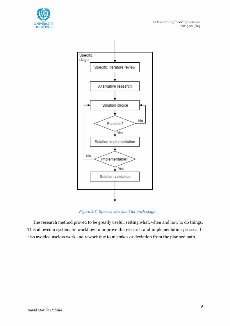
Figure 2.3. Specific flow chart for each stage.
The research method proved to be greatly useful, setting what, when and how to do things.
This allowed a systematic workflow to improve the research and implementation process. It
also avoided useless work and rework due to mistakes or deviation from the planned path.

10 David Morilla Cabello
School of Engineering Science 2019/06/04
3 Frame of reference
3.1 Computer vision
Computer vision is a wide field focused on how computers can get information from digital
images or videos. It seeks to automate tasks that the human vision can do. This discipline
started in universities that already worked on artificial intelligence such as MIT (Papert, 1966).
This project will just analyse some relevant themes studied in this field.
There is a lot of useful material to learn knowledge about this field. From web material as
free courses, academic videos, papers and articles to books. Just to mention some of them,
video courses from Prof. Peter Corke (2017), or the book Learning OpenCV (Bradski & Kaehler,
2011) are some used examples.
Something important to remark on is that some algorithms are patented, and their
commercial use depends on their license.
3.1.1 Image processing
A digitalised image is no more than a matrix with numeric values to represent the intensity of
each pixel. Digital image processing is the use of computer algorithms to transform a digital
image.
The purpose of this for computer vision is to improve the image for further analysis. These
improvements are mathematical operations over the matrix of the image in order to get a more
useful image.
A subdivision for image processing algorithms is proposed by McAndrew (2004),
distinguishing image segmentation as part of feature detection:
• Image enhancement: process the image to suit a particular application.
o Sharpening or de-blurring.
o Highlighting edges.
o Improving contrast, brightness or colours.
o Removing noise or non-desired features as reflexions.
• Image restoration: reverse the damage by a known cause.
o Motion blur.
o Optical distortions.
o Periodic interference.
11 David Morilla Cabello
School of Engineering Science 2019/06/04
All the tools used for these purposes can be expressed as mathematical functions. The
functions are normally divided into:
• Monadic and dyadic operators if it involves one or two images.
• Pixel-by-pixel, spatial and global operators if it is applied to each pixel of the image
individually, if it involves the pixel and its neighbours or if it involves all the pixels
in the image.
In order to understand this field, it is important to understand how images are represented
in the digital world. As it was mentioned before, they are mainly represented with matrices
with different values for each pixel that results in a representation of the real world. It includes
concepts as resolution (number of pixels in the image) or colour spaces (intensity, “red-green-
blue” RGB, or “hue-saturation-value” HSV).
3.1.2 Feature detection
It consists of the extraction of meaningful information from digital images. The variety of
algorithms used ranges from basic shape detector from a binary image (just with black and
white pixels) to the use of neural networks and machine learning for classifying images.
Depending on the problem, a different approach is used. In this project, the use of machine
learning was discarded because of its complexity, and some algorithms are compared in
chapter 4.1.1. Interesting analysis features are:
• Edge or corners detections. Further methods include information to deal with
transforms of the image. Some examples are the SIFT and SURF features methods.
In figure 3.1, not only corner points are obtained but also an “orientation” of these
features that keeps tracking of perspective transforms of the image.
• The topology of the image and shape analysis. These methods require some image
segmentation during the image processing in order to isolate the area to be
analysed.
• Lines and circles detection (e.g. Hough transform).
Each objective follows a different paradigm, using different mathematical approaches
(Klette, 2014). They also vary in complexity, which finally results in different computational
cost. This should be taken into account when implementing a computer vision system.

12 David Morilla Cabello
School of Engineering Science 2019/06/04
Figure 3.1 SURF features detection.
3.1.3 Tracking systems
If a problem involves movement, it could be interesting to track interesting features in the
image or even predict the motion of the object. Another approach is to detect the movement of
the camera. This is the opposite approach, as all the frame will be moving due to the motion of
the image acquisition system and it is normally applied in mobile robotics. Tracking systems
focus on track already detected features from one image to another, e.g., frames of a video.
Some of the used tools involve linear motion estimation using Kalman filters or optical flow
detectors.
The Kalman filter developed by Rudolf E. Kalman (Kalman, 1960). It is an optimal
estimation algorithm used in the space state control field. The filter estimates the state of a
system assuming statistical noise. It is widely used in guidance, navigation, control of vehicles
and trajectory planning. This filter can be used to improve the positional measure of the object,
to estimate its position in the case that the measure is lost in the next frame and to obtain an
estimation on the velocity or acceleration. The algorithm is recursive and can run in real time,
which makes this filter ideal for online state correction and estimation.
Kalman filters work well for linear systems. If the system is non-linear, a generalised
Kalman filter can be used. Recent approaches also used particle filters in order to improve the
track of the object. This method uses individual weighted statistical distributions for a set of
particles (possibilities of predictions following the statistical distributions) based on the
estimation and the measurement of the system. Iterating over the estimation of particles with
higher weights, the algorithm allows obtaining the real state. Examples of this are applied to
affine transformations in Park (2008) and further research in Kwon, Lee & Park (2009) and
Kwon et al. (2014).
13 David Morilla Cabello
School of Engineering Science 2019/06/04
Optical flow is the pattern of apparent motion of features in an image caused by the relative
motion between the camera and the points in the scene. Some of the most famous algorithms
for this purpose are the Horn-Schunck method (Horn & Schunck, 1981) and the Lucas-Kanade
method (Lucas & Kanade, 1981), being the second the most widely used. Both assume
brightness constancy for consecutive frames, small motion and coherence between the points.
These assumptions can be eased using other tools as Gaussian pyramids (Adelson et al., 1984).
Other algorithms were studied in Barron, Fleet & Beauchemin (1994).
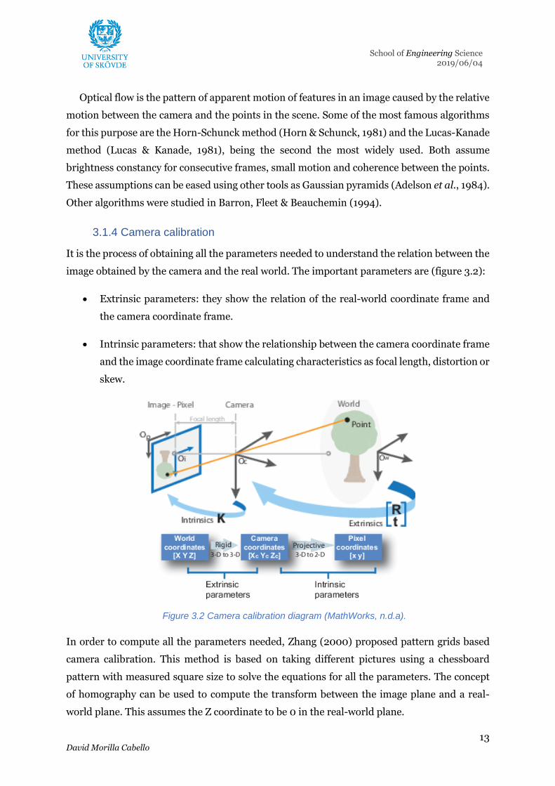
3.1.4 Camera calibration
It is the process of obtaining all the parameters needed to understand the relation between the
image obtained by the camera and the real world. The important parameters are (figure 3.2):
• Extrinsic parameters: they show the relation of the real-world coordinate frame and
the camera coordinate frame.
• Intrinsic parameters: that show the relationship between the camera coordinate frame
and the image coordinate frame calculating characteristics as focal length, distortion or
skew.
Figure 3.2 Camera calibration diagram (MathWorks, n.d.a).
In order to compute all the parameters needed, Zhang (2000) proposed pattern grids based
camera calibration. This method is based on taking different pictures using a chessboard
pattern with measured square size to solve the equations for all the parameters. The concept
of homography can be used to compute the transform between the image plane and a real-
world plane. This assumes the Z coordinate to be 0 in the real-world plane.

14 David Morilla Cabello
School of Engineering Science 2019/06/04
3.1.5 Visual servoing
This discipline consists of using computer vision in order to control the motion of a robot. One
of the first research projects that used visual servoing is Agin, G. J. (1979). The image is
processed in order to acquire visual features that are going to be used in order to reduce the
error between the current and desired target. The concepts explained are developed in
Chaumette & Hutchinson (2006) and Chaumette & Hutchinson (2007)
There are two main approaches to this problem:
• Image-based visual servo control (IBVS): the features are directly available from the
image data.
• Position-based visual servo control (PBVS): in this case, the features will be
processed estimating the 3-D pose of an object used for the control. This method is
more sensitive to camera calibration parameters as they are used for the 3-D
reconstruction.
Both approaches have their advantages and flaws. Other approaches are based on a hybrid
system with the integration of both methods. Using stereo camera systems in IBVS approaches,
the 3-D parameters can be estimated based on epipolar geometry. Apart from the methods
previously explained there are other alternatives in relation to the camera position:
• Eye-in-Hand: in this approach, the camera is in the end effector of the robot. The
camera is observing the relative position of the target in relation to the current
position of the arm. In this case, the relation between the movement of the camera
and the features is expressed in the interaction matrix. The control of the robot is
normally a velocity-based control in the joint space.
• Eye-to-Hand: in this approach, the camera is external to the robot. This gives a
global point of view of the features independent from the movement of the arm and
fixed to the world coordinate frame.
In this case, again each method has its advantages and disadvantages. Also, a collaborative
approach can also be done using two cameras to get information. Depending on the task, the
use of different alternatives can be discussed.
15 David Morilla Cabello
School of Engineering Science 2019/06/04
3.2 Industrial robot
Industrial robots are defined by ISO 8373 (International Organization for Standardization,
2012) as: “automatically controlled, reprogrammable, multipurpose manipulator,
programmable in three or more axes which can be either fixed in place or mobile for use in
industrial automation applications”. The industrial robot includes the manipulator including
the actuators and the controller, including the teach pendant and any communication
interface.
Industrial robots are normally used for manufacturing purposes. Typical application
includes pick and place, welding or painting. The end of the arm is equipped with some specific
tool for the task, normally called end effector.
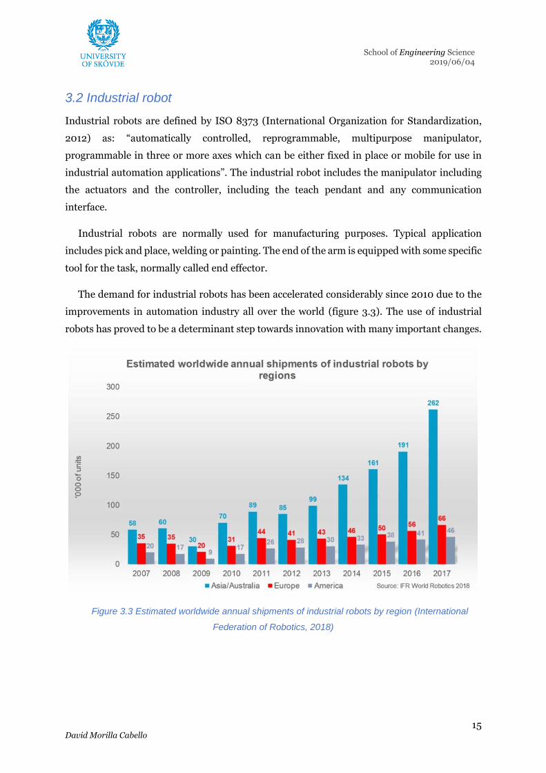
The demand for industrial robots has been accelerated considerably since 2010 due to the
improvements in automation industry all over the world (figure 3.3). The use of industrial
robots has proved to be a determinant step towards innovation with many important changes.
Figure 3.3 Estimated worldwide annual shipments of industrial robots by region (International
Federation of Robotics, 2018)

16 David Morilla Cabello
School of Engineering Science 2019/06/04
3.2.1 Control
The mechanism of the robot is controlled by its controller. The control of the robot includes
complex tasks. Some of these tasks include kinematics and dynamics application, electrics and
electronics of the actuators and sensors, feedback loops, control, pathfinding… In order to
make programming robots easier, frameworks are normally created.
Each robot manufacturer has its specific controller and they are programmed in different ways,
so each of them offers the framework for programming the robots. From the beginning of
industrial robots until now, there has been a huge lack of standardisation in robot
programming (Nnaji, 1993 and Nubiola, 2015)
Even if the programming languages for each controller are similar, the proprietary nature
of robot software has many problems. As it was stated in chapter 1.1, one of these flaws is the
integration of new features.
One solution for programming robots in a general way is using post processing tools
included in some software (e.g. RoboDK). This allows developers to code in a standard way.
After the program is coded, the software translates it to the specific robot language. This does
not allow online control of the robot, as the program is uploaded once to the robot controller.
Another solution for standardising robot programming languages is the Robotic Operating
System (ROS). ROS is a robotic middleware (i.e. software for robot software development) that
offers a framework with different tools for robot software programming. This software was
started by the Stanford Artificial Intelligence Laboratory. Its open source nature and the
constant development has made ROS gain attention from the robot industry. ROS is based on
Unix-like systems with official support for Ubuntu.
In 2012, ROS-Industrial was founded. This project focuses on industrial manufacturing
robots. Most of the common industrial manipulators have developed libraries in order to create
an interface to program robots. ROS-Industrial also offers tools for controlling grippers and
sensors or path planning.
However, ROS is a currently developing tool. Its complexity and variability make this
system hard to handle. Also, there is a lack of official standards. With the purpose of fix that
and other problems (as the implementation of real-time applications, which is currently
covered by ros_control), ROS 2.0 is being developed. Nevertheless, this version has been
considered as not enough developed.

17 David Morilla Cabello
School of Engineering Science 2019/06/04
All the information about ROS is provided in the documentation with examples and
tutorials (Wiki.ros.org, 2018). Its basic behaviour is based on the execution of tasks using
“nodes”. These nodes can publish or subscribe to “topics”, sending or receiving predefined
“messages” in order to transfer information. Each node can have more than one publisher and
subscriber. ROS also offers “server” and “client” protocols through “services” to allow a direct
connection between nodes. It is also important to mention the possibility of using global
parameters in the “param server” for using certain tools that allows an object to be available
for different programs. A brief example of the overall architecture is showed in figure 3.4. All
the programs are initialised using “launch” files in ROS packages. There is always one ROS
master in the ROS environment. The ROS master is in charge of internal tasks as the “rosout”
node.
Figure 3.4 Basic example of ROS paradigm.

18 David Morilla Cabello
School of Engineering Science 2019/06/04
3.2.2 Kinematics of a robot manipulator
An object in the space can be represented stating its 6 degrees of freedom (DOF). These are the
position and rotation from a reference frame. One of the main problems concerning robot
manipulators is to know the relation between the frames of reference of the fixed point on the
base of the robot and the tool centre point (TCP) at the other end of the mechanic chain (Ben-
Ari & Mondada, 2018). This relation is based on the position of the different joints that
compose the robot manipulator mechanism. Normally they are expressed using homogenous
transformations that represent rotations and translations in one 4x4 homogenous matrix. This
makes the representation efficient easing operations like the inverse matrix calculation. This
fields involves two main concepts: forward and inverse kinematics (figure 3.5).
Figure 3.5. Relationship between forward and inverse kinematics(El-Sherbiny, A. Elhosseini &
Y. Haikal, 2017).
Forward kinematics solves the position of the TCP depending on each joint value. The
solution is unique for each joint combination and it can be computed finding the different
transforms between each link and joint of the robot. This task is normally easy to solve if the
structure of the robot manipulator is known. It is solved using analytic methods.
Inverse kinematics tries to solve the required position of each joint to reach a certain pose
(position and rotation) in the space for the TCP. This problem is more difficult to solve.
Sometimes there is more than one solution for a single pose, different configurations of the
robot arm that results in the same position and rotation of the TCP. It can also have no solution
for a pose, or there could be singularity problems for some configuration that invalidates some
degree of freedom. As the complexity of the calculation is higher, it is normally solved using
numeric methods instead of computing the analytic solution for each case. The singularity
problems can be solved representing the coordinates frame with quaternions instead of
homogenous transforms.

19 David Morilla Cabello
School of Engineering Science 2019/06/04
A dynamic approach is also used for computing the relationship between the joint velocities
and the TCP velocity using the Jacobian Matrix. This is useful for velocity and torque control
of a robot. It also has a forward and inverse focus.
3.2.3 Simulation
In order to save time and costs and reduce hazards in the real world, virtual simulation
models are implemented for offline programming. The simulation can be as detailed as
desired. It can include just a visualisation of the robot arm or the complete work cell (figure
3.6), actuators and sensors behaviour, a physics engine for collision detection or dynamics.
Normally, the robot manufacturer offers its own software for simulation, including the
available manipulator models and some objects modelling. There is also much other software
for robot simulation. Controlling simulated robots is normally easier than controlling a real
robot, this is the reason why there is more third party (open source or proprietary) software
for robot simulation.
Figure 3.6 Example of a UR3 simulation in Gazebo.
Robot models for simulation are normally represented by the Universal Robots Description
Format (URDF). This format is an XML format file that contains all the information needed
for simulating the robot. As URDF files can become complicated, they can be implemented
using XACRO (XML Macros) files, a way of implementing XML files using macros. However,
new formats are being developed in order to include more descriptions, as the environment for
the robot (terrain, lightning, objects…) or even physics. The most prominent example is the
SDF.
Nowadays simulation has become a necessary part with the development of Industry 4.0.
Some of the fields where simulation is applied are robot offline programming, model validation
or optimization.

20 David Morilla Cabello
School of Engineering Science 2019/06/04
4 Literature review
In order to get a general overview of the previous work in the field of this project, other
scientific documents are analysed in this chapter. The analysis is done for each part of the
project.
4.1 Computer vision alternatives
4.1.1 Algorithms
There are many surveys in moving object tracking due to the important and recent
development of the field. One of them is Balaji & Karthikeyan (2017) where state of the art
algorithms for this task can be seen. The methodology and mathematical approach of each
algorithm are widely varied. Different papers have also been analysed to get into real
implementations. Normally, the algorithm used depends on the task to be performed and the
complexity, robustness and reliability of the desired system.
For basic detection tasks, a simple blob analysis is used in Gornea et al. (2014) with colour
filtering and estimation of the position using geometrical parameters and assuming a ball
object. Canali et al. (2014) also performed a blob analysis based on the centre of mass in order
to calculate grasps points for a robot tool using the silhouette of the detected blob. In order to
compute basic geometric shapes, Reddy & Nagaraja (2014) used the compactness of the blobs
detected. The centroid and orientation are calculated assuming the geometric shape.
Roshni & Kumar (2017) used a pre-train image for feature match when it comes to
recognising the object. The specific feature detector is not specified. However, in Wang et al.
(2015) it is stated that SURF features detection is used for classifying the specific object. These
two cases used saved images for the feature match. The centroid can be specified in the
reference image or computed using a minimum bounding rectangle for the features and
rotating callipers for the orientation as in the second case.
For fast moving objects, Cigliano et al. (2015) developed a complex system. Its literature
review offers an overview of flying object detection and tracking methods. In this document,
the inter-frame difference has been used. Frese et al. (2001) and Ribnick et al. (2007) can be
used as simpler examples for this algorithm. Cigliano et al. however, also used the Hough
transform for round objects detection and many other algorithms to improve the measurement
and the tracking. A similar approach is also used in Golz & Biesenbach (2015) for detecting
which chess piece has been moved.

21 David Morilla Cabello
School of Engineering Science 2019/06/04
Further algorithms use foreground detectors, normally for people or vehicle detection and
tracking (e.g. video surveillance). Optical flows are also used for detecting moving objects and
perform the tracking.
Other tracking algorithms used are Kalman filter implementations as in Montúfar et al.,
(2017). In case that a non-linear tracking is required, the most common options are:
implementing a generalised Kalman filter or using particle filters. Husain et al. (2014)
compared their implementation of a particle filter with the available in Point Cloud Library,
the most used algorithm for that moment. Spatio-temporal context (STC) algorithms are also
used for tracking (Zhang et al., 2013). In this case, Zhao, Huang & Chen (2017) also improved
the algorithm with their Improved spatio-temporal context (ISTC), which seems to
outperform the previous one.
It is important to remark the recent usage of machine learning and neural networks as well
as the fuzzy-logic-based controllers in computer vision and visual servoing tasks. However,
these approaches are out of the scope in this project (Hwang, Lee & Jiang, 2017, Siradjuddin
et al., 2014 and Mekki & Kaaniche, 2016).
4.1.2 Software
Regarding the literature studied in chapter 4.1.1. Normally, the software used for the projects
studied is not specified in depth. Most of the projects use self-created programs with or without
the help of already existing libraries (Pochyly et al., 2017 and Husain et al., 2014). The most
common languages used, if stated, are C/C++, C# or Python.
The most used software is the OpenCV library (Wang et al., 2015). This is an open source
C/C++ library for computer vision. It is also available for python. Most of the available
programs for computer vision also uses some tools from OpenCV (e.g. MATLAB uses OpenCV
implementation of SURF features method).
Research into industry real cases is difficult through official scientific resources. For this
research, case studies from different automation websites have been studied. Currently,
offering an individual solution from automation, electronic or camera companies is the most
common approach (ABB ROBOTICS, 2018). Normally with the use of standard products
created by those companies (KUKA, n.d.) or in collaboration with other companies (Universal
Robots, n.d.a). If the company has a long history using computer vision, it could have self-
created software libraries. These approaches require a minimum knowledge in the field of
computer vision but lack of flexibility.
22 David Morilla Cabello
School of Engineering Science 2019/06/04
However, there are also used frameworks used for computer vision. One example is the
MATLAB Computer Vision Toolbox (Gornea et al., 2014). This toolbox offers an already
implemented function in a high level programming language. Due to the academic interest of
MATLAB, some articles researched have been specifically analysed because of the use of this
software. Even if MATLAB is intrinsically slower than programs made using OpenCV libraries
directly (Matuska, Hudec & Benco, 2012), it offers other facilities. Some of them are an easy
programming language, visual interfaces and apps that are more user-friendly. There are other
examples of libraries and software for computer vision, they are compared in chapter 6.
Other already existing frameworks as Octave or Mathematica have not been found in any
projects in an easy way and their functionalities have been considered as not enough for the
aim of this project.
4.1.3 Hardware
Regarding the devices used for image acquisition, it was not determinant in any of the cases
unless some specific feature is required (e.g. 3D vision). The only restrictions found are:
• Decent quality for improving the image analysis (320x240/640x480 px). However,
a bigger resolution requires more demanding computing, which makes the
algorithm unable to perform in online tasks.
• Good frame-rate acquisition (30 fps at least). It should not be a bottleneck in image
processing. In fast-tracking cases, the frame-rate must be higher (increasing up to
120 fps).
• In case of fast image recognition, a global shutter is needed in order to avoid
deformation caused by rolling shutter.
In many cases, industrial cameras (e.g. GigE, Matrox and Point Grey) are used (Pochyly et
al., 2017). They tend to be more expensive, but their extremely good specifications make them
suitable for multiple projects in academic research.
23 David Morilla Cabello
School of Engineering Science 2019/06/04
4.2 Robot control
There are two main groups in the robot manipulators analysed in the literature. The robot can
be created by a university or a research team. In this case, the robot is controlled with the
specific controller created for it. However, the manipulators can be purchased robots from
manufacturers (e.g. ABB, Universal Robots, KUKA, Staubli…). In this case, the way of
controlling it can vary. Not all the literature mentions the way of controlling the robot.
However, some information can be extracted. In some cases, the robots are connected to the
main software for the controller (Roshni & Kumar, 2017 and Wang et al., 2015). It can also be
connected to the controller directly (Golz & Biesenbach, 2015, Zhao, Huang & Chen, 2017 and
Mao, Lu & Xu, 2018). In other cases, ROS is used (Zhang et al., 2018). In the specific case of
Universal Robots, Andersen (2015) analysed the different methods for controlling these robot
arms. The URScript method is applied in different ways by third-party programs as some
Universal Robots interfaces for MATLAB using python (Kutzer, 2019) and for the package
ros_control using the package distributed from Universal Robots ur_modern_driver
(Andersen, 2015).
24 David Morilla Cabello
School of Engineering Science 2019/06/04
5 Overall design of the system
The design of the system is created to follow a modular structure in order to study each part
separately. All the modules are explained in the following chapters. Figure 5.1 shows the
scheme of the system. It consists of the following parts:
• Computer vision system: comprised of all the needed tools to acquire and process
the image as well as to compute the centroid of the object. The final output is the
coordinates (position and orientation) of the centroid in the real world 2D plane. It
is divided into these subsystems:
o The image acquisition system with the hardware and the software needed.
This part acts as a source for the images. The output is the image captured
by the camera.
o The image processing stage which modifies the image in order to improve
the analysis part.
o The image analysis that extracts features and data from the processed image.
In this case, it is responsible for obtaining the centroid and orientation.
o The tracking system uses algorithms to filter the position of the object and
solves occlusion and short fading of the centroid. Its output is the final
position and orientation.
o The frame of reference conversion. This function uses the camera calibration
parameters to convert transform the representation of the point from the
image coordinate frame to the real-world coordinate frame.
• Robot control: this part performs the computation of the joint values for the robot
from the centroid and orientation. It includes the inverse kinematics module and
the other functions in order to improve the control of the robot.
• Robot simulation: it receives the joint values from the robot control and simulates
the robot environment and behaviour. This is used to verify and validate the system
before using it against a real robot.
• Robot interface: it receives the joint values and communicates with the robot
controller in order to perform the movement of the robot.

25 David Morilla Cabello
School of Engineering Science 2019/06/04
Figure 5.1 System structure overview.

26 David Morilla Cabello
School of Engineering Science 2019/06/04
6 Computer vision system
6.1 Software comparison and selection
Based on the literature review mentioned in chapter 4 and internet research (official software
webpages, forums…) various alternatives for implementing the computer vision system are
compared in table 6.1. The comparison process only includes software that fulfils the following
features as they were found interesting for the aim of the project:
• The inclusion of optimal algorithms to program and implement computer vision tools
or programs. This means, that many of the already existing algorithms and method for
computer vision should be already implemented or easily implementable. The
alternatives have not been analysed in a strict way in this requirement as it would
enlarge too much the research process, the analysis shows that they include enough of
the algorithms needed for implementing many solutions.
• The possibility of interfacing the software with the robot control system. The interface
should be easy to implement in order to use the system as a block in a larger system.
• The maintenance by a community or company is not a basic requirement but was a
crucial aspect of the comparative process. Abandoned software or unpopulated user
communities make the software difficult to evolve and adapt to future matters.
• The flexibility for implementing new and flexible algorithms, tools, functions… This
allows extending the software, covering new upcoming problems, technologies and
approaches by the users.
All the software alternatives for computer vision explained in table 6.1 fulfils the previously
mentioned requirements. However, they implement similar functionalities, focusing on
improving specific characteristics. Most of them are libraries implemented in C++ and allow
for cross-platform usage. It can also be seen the importance of open source software in this
area. Even if OpenCV is the most used library, other libraries are also used and maintained by
the community. The license can depend sometimes on the algorithms used as some of them
have different licenses. Each project can be individually analysed with the source link provided.

27 David Morilla Cabello
School of Engineering Science 2019/06/04
Software Category Language Open
source
Main focused
OS
License Additional notes
MATLAB Integrated
development
environment
(IDE)
MATLAB No Windows, Mac OS
X, GNU/Linux
Proprietary Compatible with
OpenCV and
prepared for Code
Generation in
C/C++.
Communication
with ROS
implemented.
OpenCV Library C++ (Python
and Java
interfaces)
Yes Multiplatform
(Windows, Mac
OS X, GNU/Linux
and Android)
BSD 3-clause
(except some
tools)
Most used software
by the community.
VXL Libraries C++ Yes Multiplatform Zlib/libpng Attends to improve
IUR and TargetJr
systems.
BoofCV Library Java Yes Multiplatform Apache 2.0
AForge.NET Framework C# Yes Multiplatform LGPL v3
(except
AForge.Video.
FFMPEG
component)
Old posts and news
in the official
webpage and
source.
ccv Library C Yes Multiplatform BSD 3-clause Attends to improve
old computer vision
implementations.
Visual Servoing
Platform (ViSP)
Library C++ Yes Multiplatform GNU GPL v2
or Professional
edition
Modular software
with multiple
shared or static
libraries. Allows
third-party libraries
usage.
Vision 4
Robotics (V4R)
Library C++ Yes Multiplatform
(Debian package
offered)
Dependency
dependant
Based on Point
Cloud Library
(focused on RGB-D
tasks).
Table 6.1 Software comparison for computer vision.
28 David Morilla Cabello
School of Engineering Science 2019/06/04
Once the alternatives have been analysed, the most suitable software for the task are
OpenCV and MATLAB. Some of the reasons are:
• They have the biggest variety of tools and features.
• They have the best integration with different operating systems and graphical
processing units (GPU) that improves the efficiency of image computing.
• The languages are familiar to the student, especially in the case of MATLAB.
However, other options could also be taken into consideration for different situations. If the
user is more familiar with a different programming language or a different library structure is
preferred.
Comparing these two alternatives, on one hand, we have that MATLAB has a friendly IDE
that offers GUI tools, fast inbuilt algorithms and Simulink environment. This software allows
for easy and fast implementation. However, it has a lack of performance when not inbuilt
algorithms are used. MATLAB is also a proprietary software with high license prices. On the
other hand, OpenCV consists of source code in C++ with wrappers in other languages. This
increases the performance compared to MATLAB, but the complexity of the programming is
increased. Especially if the user is not familiar with the programming languages. Also, it is open
source with BSD3 clause, so there is not any cost associated.
In this case, some reasons to use MATLAB are the familiarity with the programming
language, a user-friendly environment, out-of-the-box tools and the ownership of MATLAB
from The University of Skövde (there are not any additional expenses in licenses acquisition).
The implementation of the project is composed of different systems. MATLAB also offers tools
to implement the following systems (robot control and robot simulation). It also allows the
possibility of interfacing with ROS. Therefore, the software is reduced in variability. As
OpenCV is a library, it also allows the connection with ROS using the corresponding libraries
and implementing the code directly. However, more research should be performed to find a
solution to the robot control system.
An interesting procedure is to prototype solutions in MATLAB and port the solution to
OpenCV. This is eased as the functions and algorithms used for both software are similar. It is
also known that MATLAB uses some of the functions from OpenCV as inbuilt code.
29 David Morilla Cabello
School of Engineering Science 2019/06/04
6.2 System implementation
There are two common approaches to implement a system in MATLAB. The first one consists
of MATLAB scripts, the second one is using Simulink environment. Both are equally supported
in MATLAB. However, once the system implementation was started, some of their differences
came out.
6.2.1 MATLAB scripting and Simulink comparison
MATLAB scripting is the basic way to go in MATLAB. There are a few more functions and
classes implemented compared to Simulink and they allow more control and flexibility. The
use of conditions, mathematical operations and logic loops are similar to other programming
languages. Working with structs and multiarray is also easier with a basic object-oriented
approach with a dot to access the attributes and methods.
In the case of Simulink, some of the functions are not available and can just be implemented
with interpreted or generated code from MATLAB (explained in chapter 6.2.2). This is limited
in most of the cases, which can complicate the implementation of particular solutions.
Conditions, mathematical operations and loops are different from the common programming
language and require thinking in a different way. The management of multiarray and structs
is performed through signal and buses management, which is less intuitive than MATLAB
scripting. Simulink models are also prepared for running in real time and use continuous time.
Another characteristic to consider is that all the code used in Simulink is prepared for code
generation, while not all the code used in MATLAB scripting allows this.
As this implementation is an online control, Simulink has been chosen. This decision is also
based on further steps as it also includes the chance of using Simscape Multibody, a plugin for
simulating physic bodies that have been used for the virtual robot simulation. However, a
prototype in MATLAB scripting code has been created in order to prove the possibility of the
implementation using that method too.
6.2.2 Model description
The model consists of many blocks that are explained above, the general diagram can be seen
in figure 6.2, each part is explained in detail later. The image is captured using the Image
Acquisition Toolbox and the winvideo adapter from MATLAB. The camera used is Intel Real
Sense Depth Camera 435. This camera was selected as the features are enough for this project
and to ease a future implementation of 3D image recognition in the project. The camera is
placed in a fixed position. This means that the approach used is Eye-to-Hand and PBVS. The
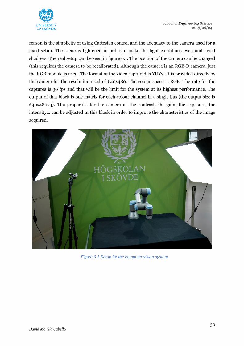
30 David Morilla Cabello
School of Engineering Science 2019/06/04
reason is the simplicity of using Cartesian control and the adequacy to the camera used for a
fixed setup. The scene is lightened in order to make the light conditions even and avoid
shadows. The real setup can be seen in figure 6.1. The position of the camera can be changed
(this requires the camera to be recalibrated). Although the camera is an RGB-D camera, just
the RGB module is used. The format of the video captured is YUY2. It is provided directly by
the camera for the resolution used of 640x480. The colour space is RGB. The rate for the
captures is 30 fps and that will be the limit for the system at its highest performance. The
output of that block is one matrix for each colour channel in a single bus (the output size is
640x480x3). The properties for the camera as the contrast, the gain, the exposure, the
intensity… can be adjusted in this block in order to improve the characteristics of the image
acquired.
Figure 6.1 Setup for the computer vision system.
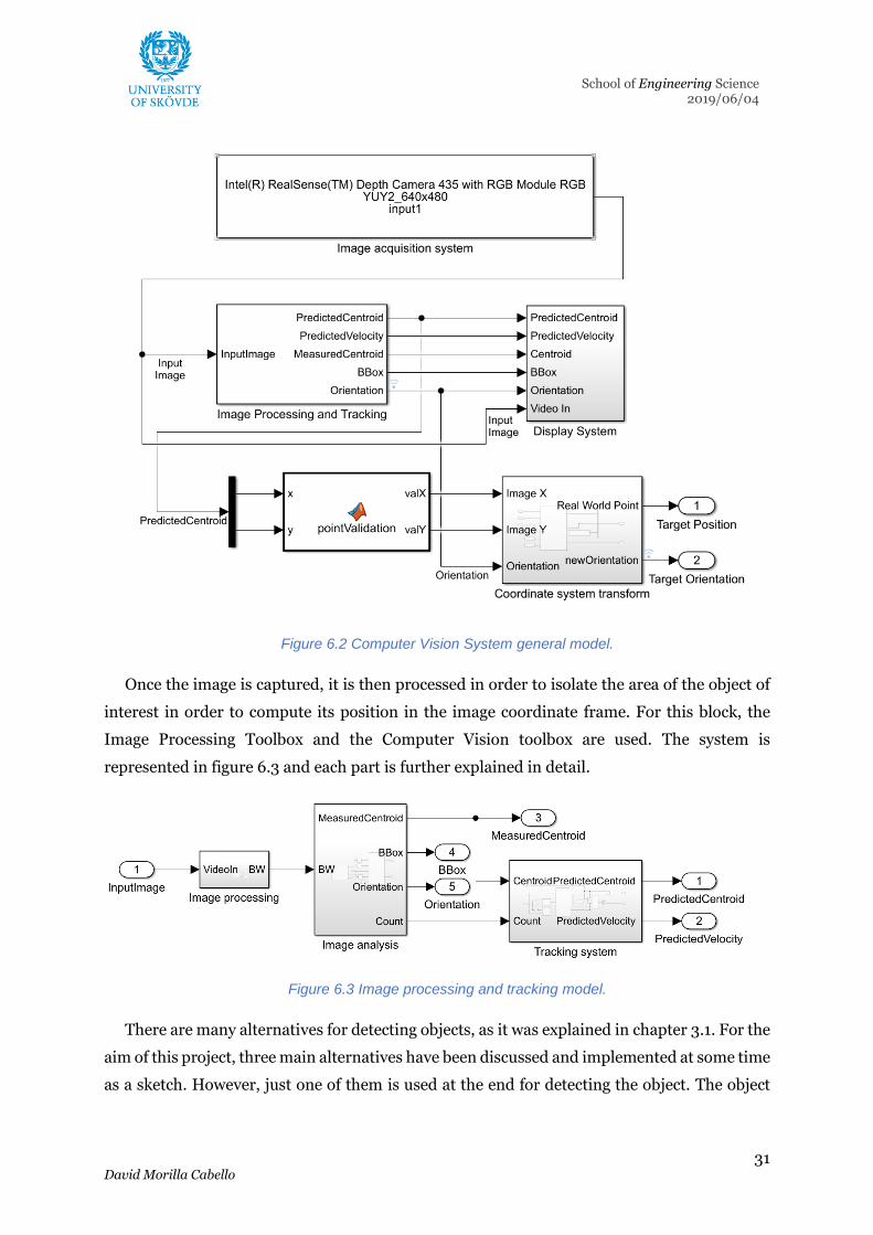
31 David Morilla Cabello
School of Engineering Science 2019/06/04
Figure 6.2 Computer Vision System general model.
Once the image is captured, it is then processed in order to isolate the area of the object of
interest in order to compute its position in the image coordinate frame. For this block, the
Image Processing Toolbox and the Computer Vision toolbox are used. The system is
represented in figure 6.3 and each part is further explained in detail.
Figure 6.3 Image processing and tracking model.
There are many alternatives for detecting objects, as it was explained in chapter 3.1. For the
aim of this project, three main alternatives have been discussed and implemented at some time
as a sketch. However, just one of them is used at the end for detecting the object. The object

32 David Morilla Cabello
School of Engineering Science 2019/06/04
detectors normally use some algorithm to convert an image in a binary image which is just pure
black and pure white (represented by 0 and 1) in order to simplify the analysis step.
The discussed alternatives were:
• Colour-based detection using colour threshold: this method applies a threshold to
each colour channel separately so just the colour margin selected is white.
• Background detector: this method creates a background model using Gaussian
mixture models. Then, it compares the model with new frames and the differences
are detected as objects.
• Feature detection using SURF method: this method does not create a binary image.
Instead, it compares features from a reference image with the camera frame and
computes the transformation from the reference to the object by detecting a high
number of feature coincidences.
In this case, in order to have the most robust system, colour-based detection has been
implemented. The Colour Threshold application in MATLAB has been used to tune the colour
filter in live mode. This application creates a MATLAB script that can be implemented in
Simulink as a MATLAB function. This method is stable against changes in the light conditions
when using HSV colour space and does not depend on the movement of the object.
Once the image is processed by the colour detector, it becomes a binary mask with pixel
values of zero (black) or one (white). In order to isolate the object of interest, the morphological
operations open and close are applied. The first one applies a extrude operation and a dilation
operation in that order with a predefined shape. This process eliminates any area that cannot
contain the specified shape. The selection of the shape can be improved depending on the
object to detect and its pixel size is strongly dependent on the camera resolution. The second
operation applies the same morphological functions in the opposite order. It applies first the
dilation operation and then the extrusion with the pre-defined shape. This operation fills the
holes that can be contained in the specified pattern that is enclosed in a bigger shape and
improves the border contour of that shape. The result of both operations is a binary mask with
reduced noise and close shape of the moving object. In figure 6.4, the different results are
shown. The results are the mask obtained with the colour filter (left-bottom), the mask
obtained after morphological operations (left-top) and the final result for centroid and
orientation (right). Figure 6.5 shows the Simulink system for the processing process.

33 David Morilla Cabello
School of Engineering Science 2019/06/04
Figure 6.4 Displayed results obtained with the Computer Vision System.
Figure 6.5 Image processing model.
After the mask is obtained, it is processed by the blob analysis block. This block analyses
characteristics from the resulting shapes called blobs. Some of these characteristics are area,
bounding box, centroid position, orientation or number of blobs. The algorithms used are
explained in Corke (2017). The block also has many configurable parameters such as the
maximum number of blobs or the maximum and the minimum area of the blobs in order to
improve the measure and detect outliers.

34 David Morilla Cabello
School of Engineering Science 2019/06/04
Some details about the characteristics are:
• The centroid is computed using the concept of centre of mass.
• The area is measured in pixels.
• The bounding box is a rectangle that encloses the max and min pixel for each image
axis.
• The orientation is deducted using the equivalent ellipse representation of the shape.
It represents the angle between the x axis in the image and the major axis of the
equivalent ellipse.
The outputs from this block are the centroid, the bounding box, the orientation and the
number of blobs detected. The angular position will not vary in the movement of the object.
The centroid and the orientation are filtered using a threshold method. It is implemented with
a MATLAB function. It compares the centroid position and the orientation value with the
previous centroid and orientation, if the difference is bigger than a margin, the used centre or
orientation will be the previous one. This allows for avoiding false or dangerous measurements.
In the case of the orientation, this also avoids 180º changes due to symmetrical objects. This
system is represented in figure 6.6.
Figure 6.6 Image analysis model.
As the movement of the centroid is supposed to be uniform (constant velocity), a Kalman
filter is applied to its measure. The tracking filter system (figure 6.7) uses a state flow chart in
order to control its use. The three states (figure 6.8) are searching for a new object, tracking
and correcting with the new measures and just tracking because the measure was lost.

35 David Morilla Cabello
School of Engineering Science 2019/06/04
Figure 6.7 Tracking model.
Figure 6.8 State flow chart for the tracking system.
The system will stay in the searching mode until an object is detected (count greater than
0). In this mode, the output centroid is the measured one. If there is not any detected centre,
the output is (-1, -1) for the position. When an object is detected a counter starts. If the counter
reaches a certain number of cycles detecting the object, the detection is considered as valid and
the state changes to tracking and correcting. The Kalman filter starts working correcting its
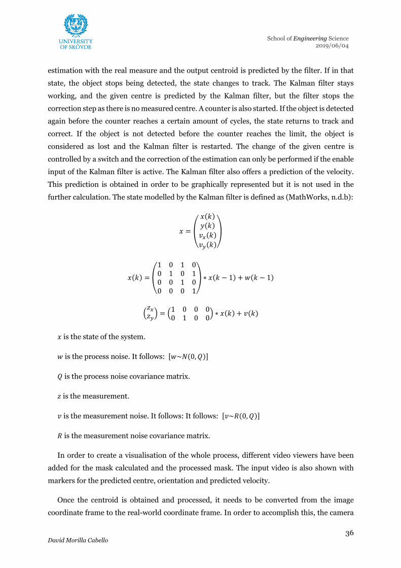
36 David Morilla Cabello
School of Engineering Science 2019/06/04
estimation with the real measure and the output centroid is predicted by the filter. If in that
state, the object stops being detected, the state changes to track. The Kalman filter stays
working, and the given centre is predicted by the Kalman filter, but the filter stops the
correction step as there is no measured centre. A counter is also started. If the object is detected
again before the counter reaches a certain amount of cycles, the state returns to track and
correct. If the object is not detected before the counter reaches the limit, the object is
considered as lost and the Kalman filter is restarted. The change of the given centre is
controlled by a switch and the correction of the estimation can only be performed if the enable
input of the Kalman filter is active. The Kalman filter also offers a prediction of the velocity.
This prediction is obtained in order to be graphically represented but it is not used in the
further calculation. The state modelled by the Kalman filter is defined as (MathWorks, n.d.b):
𝑥 =
(
𝑥(𝑘)
𝑦(𝑘)
𝑣𝑥(𝑘)
𝑣𝑦(𝑘))
𝑥(𝑘) = (
1 0 1 00 1 0 10 0 1 00 0 0 1
) ∗ 𝑥(𝑘 − 1) + 𝑤(𝑘 − 1)
(𝑧𝑥𝑧𝑦) = (
1 0 0 00 1 0 0
) ∗ 𝑥(𝑘) + 𝑣(𝑘)
𝑥 is the state of the system.
𝑤 is the process noise. It follows: [𝑤~𝑁(0, 𝑄)]
𝑄 is the process noise covariance matrix.
𝑧 is the measurement.
𝑣 is the measurement noise. It follows: It follows: [𝑣~𝑅(0, 𝑄)]
𝑅 is the measurement noise covariance matrix.
In order to create a visualisation of the whole process, different video viewers have been
added for the mask calculated and the processed mask. The input video is also shown with
markers for the predicted centre, orientation and predicted velocity.
Once the centroid is obtained and processed, it needs to be converted from the image
coordinate frame to the real-world coordinate frame. In order to accomplish this, the camera

37 David Morilla Cabello
School of Engineering Science 2019/06/04
parameters are needed. These parameters are computed calibrating the camera. In order to
calibrate the camera, MATLAB includes an application that allows computing all these
parameters taking images and using the checkerboard method mentioned in chapter 3.1.4.
Then, the application creates a MATLAB script to automate the calculation of these parameters
using the images taken and creates the correspondent variables in the MATLAB workspace.
This script is executed in the initFcn callback function of the Simulink model, this means, each
time it is compiled. The transform of the coordinate frame can be seen in figure 6.9 and is
applied by the “image2world” function. It applies the homography from the image plane to the
real-world plane using the inverse intrinsic and extrinsic matrices. This allows obtaining the
equivalent coordinates and orientation for the object in the real-world frame.
Figure 6.9 Transform of the coordinate frame.
Before the image2world function, there is another function called pointValidation. This
function filters the result of the centroid if it is not a valid point for the real world (out of the
workspace) or if its values are (-1, -1), the output when there is not any detected centroid. If the
centroid is valid, the output is that point. If the point is not valid, the output is a neutral position
that works as a rest pose for the robot. The orientation is also restricted to the first quadrant
as the tool is considered symmetrical.
Finally, the result is the X and Y coordinate in the real-world plane of the table in front of
the robot as well as the equivalent orientation of the object as a rotation of the Z axis. The
orientation is introduced later in the coordinates as a rotation of the TCP. The Z coordinate is
fixed in this case in order to offer a safe distance between the end tool and the object on the
table.

38 David Morilla Cabello
School of Engineering Science 2019/06/04
7 Robot control
The robot control system consists of all the algorithms used to transform the target position
into joint values. It also includes methods to avoid dangerous or unexpected movements of the
robot arm. Even if some alternatives have been analysed, one determining factor is the use of
MATLAB in the computer vision system (chapter 6).
7.1 Alternatives analysis
There are different alternatives for controlling the robot. In this case, the most obvious
approach is using Simulink as it is the already in use software. There are also different solutions
in Simulink. One of them is using the already implemented inverse kinematic solver block. This
solution is based on numerical methods and explained in detail later, as it was the chosen one.
Different solutions use the Jacobian Matrix of the robot arm that can be computed with
another already created block. This solution implements a control based on the velocity instead
of the position of the joints. Another alternative is using a MATLAB script, which allows using
an analytic inverse kinematic solver. In this alternative, the solver has the drawback of being
different for each robot arm used. Besides using MATLAB, ROS can be used for this task. There
are some tools such as MoveIt! for solving inverse kinematics. MoveIt! also uses numerical
algorithms that are included in the software to obtain the position of the joints. However, this
software is more complex allowing trajectory calculation or obstacle avoidance. It would
require further research in this software. Using MoveIt! would imply sending the position and
rotation of the target to ROS from the program used for computer vision. In Simulink, this can
be done using the publisher block, which is explained in chapter 9. Of course, the option of
using self-code exists but has not been analysed in detail as it is out of the scope for this report.
The chosen solution was using the inverse kinematic solver as mentioned. This is the most
compatible solution with the computer vision system because it is already implemented in
Simulink and is a reliable method for the task.
7.2 System implementation
The robot control system consists of the inverse kinematic solver provided by MATLAB and
some pre-processing functions for the target position and orientation (figure 7.1). The inverse
kinematic solver uses the rigid body tree generated by MATLAB with the URDF file. This
generation is computed in the initFcn callback function when the model is compiled. For this
case, the URDF file is provided by Universal Robots for the UR3 in the package ur_description
for ROS. In this package, there are XACRO files for all Universal Robots arms. The XACRO file
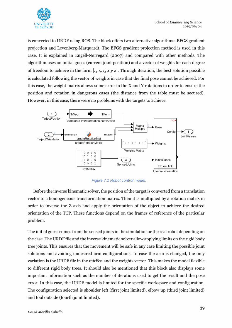
39 David Morilla Cabello
School of Engineering Science 2019/06/04
is converted to URDF using ROS. The block offers two alternative algorithms: BFGS gradient
projection and Levenberg-Marquardt. The BFGS gradient projection method is used in this
case. It is explained in Engell-Nørregard (2007) and compared with other methods. The
algorithm uses an initial guess (current joint position) and a vector of weights for each degree
of freedom to achieve in the form [𝑟𝑥 𝑟𝑦 𝑟𝑧 𝑥 𝑦 𝑧]. Through iteration, the best solution possible
is calculated following the vector of weights in case that the final pose cannot be achieved. For
this case, the weight matrix allows some error in the X and Y rotations in order to ensure the
position and rotation in dangerous cases (the distance from the table must be secured).
However, in this case, there were no problems with the targets to achieve.
Figure 7.1 Robot control model.
Before the inverse kinematic solver, the position of the target is converted from a translation
vector to a homogeneous transformation matrix. Then it is multiplied by a rotation matrix in
order to inverse the Z axis and apply the orientation of the object to achieve the desired
orientation of the TCP. These functions depend on the frames of reference of the particular
problem.
The initial guess comes from the sensed joints in the simulation or the real robot depending on
the case. The URDF file and the inverse kinematic solver allow applying limits on the rigid body
tree joints. This ensures that the movement will be safe in any case limiting the possible joint
solutions and avoiding undesired arm configurations. In case the arm is changed, the only
variation is the URDF file in the initFcn and the weights vector. This makes the model flexible
to different rigid body trees. It should also be mentioned that this block also displays some
important information such as the number of iterations used to get the result and the pose
error. In this case, the URDF model is limited for the specific workspace and configuration.
The configuration selected is shoulder left (first joint limited), elbow up (third joint limited)
and tool outside (fourth joint limited).

40 David Morilla Cabello
School of Engineering Science 2019/06/04
8 Robot simulation
Simulating the model helps both in the validation and verification process. That is why the
simulating model was not implemented after the previous step was completely finished, but it
also helped for its implementation.
Three different simulations were performed in order to get a step-by-step approach to the
final system. These three simulations were:
• Simulation of the rigid body tree in Simulink using Simscape Multibody.
• Simulation of a model of the robot in Gazebo in ROS.
• Simulation of a replicate model of the real robot with the Universal Robots Simulator
(URSim).
They are introduced in this chapter. However, some concepts used for their implementation
are explained in chapter 10 related to the robot interface involving ROS.
8.1 Simulation in Simulink with Simscape Multibody
The first simulation was implemented in Simulink. Simulink uses Simscape Multibody for this
purpose. This toolbox enables the building of physical component models based on physical
connections. The model receives the joint values command. Those values are transformed into
physical signals and introduced as the joint position in the correspondent blocks. The current
position of each joint can also be sensed and used in the inverse kinematic solver (chapter 7).
A visualisation of the simulation is displayed in MATLAB.
Figure 8.1 General view of the Simscape Multibody simulation model.

41 David Morilla Cabello
School of Engineering Science 2019/06/04
The diagram of the model is shown in figure 8.1. The general model consists of the basic
definition of the world frame of reference, the mechanism configuration to specify properties
such as the gravity value and the solver configuration. Simscape Multibody is based in a
sequence of link blocks and joint blocks. The link blocks establish the transform between the
bodies and other properties like mass, inertia, and the 3D mesh used for the representation
(example in figure 8.2). The joint blocks are different for each type of joint (prismatic, revolute,
weld, spherical…) it also specifies properties shown in figure 8.3. After the three basic blocks
mentioned above, a link between the world frame of reference and the defined world is used.
In this case, that transformation is an identity. After that, two systems are related to the world
frame of reference. One is the UR3 arm simulated model, and the other is a representation of
the detected object. The second model is used for displaying the recognised object and prove
that the arm is above it. This system was implemented because of its simplicity. It is just a
circular body without any dynamic property related to the world frame of reference by the
position of the centroid. The UR3 model is shown in figure 8.4.
Figure 8.2 Example of link block autogenerated from UR3 model.

42 David Morilla Cabello
School of Engineering Science 2019/06/04
Figure 8.3 Properties of the revolute joint block from the UR3 model.
The UR3 model is automatically generated from the URDF file using the MATLAB function
smimport. The model can be adjusted afterwards. In figure 8.4 it can be seen how the joint
commands are introduced and how the sensed position of the joints is an output to the inverse
kinematic block. It is important to notice the use of rate converters before and after this block
in order to adjust the sampling time with the rest of the system.

43 David Morilla Cabello
School of Engineering Science 2019/06/04
Figure 8.4 UR3 robot autogenerated model in Simscape Multibody.
This model simulates physics and dynamic behaviours included in the URDF file. However,
it does not simulate other behaviours such as the collision between rigid elements (the bodies
can move into other bodies), the behaviour of the motors and the robot controller. This model
can also be improved in order to have a more realistic behaviour detecting collisions or even
simulating the complex behaviours using Simscape tools. In this case, this was not considered
as other simulators were going to be used. This simulation was mostly used as a modelling tool
for the robot control system.
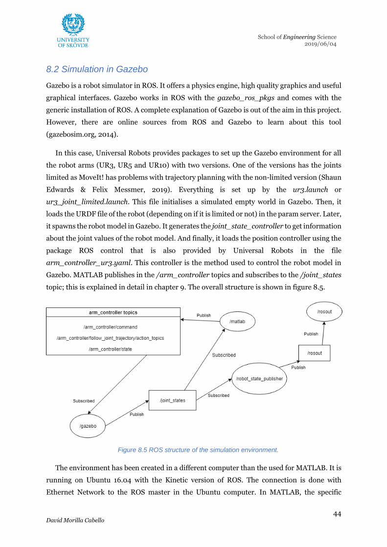
44 David Morilla Cabello
School of Engineering Science 2019/06/04
8.2 Simulation in Gazebo
Gazebo is a robot simulator in ROS. It offers a physics engine, high quality graphics and useful
graphical interfaces. Gazebo works in ROS with the gazebo_ros_pkgs and comes with the
generic installation of ROS. A complete explanation of Gazebo is out of the aim in this project.
However, there are online sources from ROS and Gazebo to learn about this tool
(gazebosim.org, 2014).
In this case, Universal Robots provides packages to set up the Gazebo environment for all
the robot arms (UR3, UR5 and UR10) with two versions. One of the versions has the joints
limited as MoveIt! has problems with trajectory planning with the non-limited version (Shaun
Edwards & Felix Messmer, 2019). Everything is set up by the ur3.launch or
ur3_joint_limited.launch. This file initialises a simulated empty world in Gazebo. Then, it
loads the URDF file of the robot (depending on if it is limited or not) in the param server. Later,
it spawns the robot model in Gazebo. It generates the joint_state_controller to get information
about the joint values of the robot model. And finally, it loads the position controller using the
package ROS control that is also provided by Universal Robots in the file
arm_controller_ur3.yaml. This controller is the method used to control the robot model in
Gazebo. MATLAB publishes in the /arm_controller topics and subscribes to the /joint_states
topic; this is explained in detail in chapter 9. The overall structure is shown in figure 8.5.
Figure 8.5 ROS structure of the simulation environment.
The environment has been created in a different computer than the used for MATLAB. It is
running on Ubuntu 16.04 with the Kinetic version of ROS. The connection is done with
Ethernet Network to the ROS master in the Ubuntu computer. In MATLAB, the specific

45 David Morilla Cabello
School of Engineering Science 2019/06/04
message for the /arm_controller topic must be created from the joint values. The information
from the /joint_states topic has to be processed in order to obtain the joint values in a vector
format. These tasks are performed by the ROS interface system and explained in detail in
chapter 9.
This simulation offers more dynamic characteristics such as the collision simulation and
allows to validate the ROS interface between MATLAB and ROS. Even if this simulation shows
the behaviour of the controller, it does not simulate the behaviour of the actual controller in
the robot.
8.3 Simulation using URSim
This simulation replicates the behaviour of the real robot. It is implemented in a virtual
machine provided by Universal Robots and the program for the UR3 robot arm. The virtual
machine was configured to be in the same network as the other computers. This allows the
ROS system to connect with URSim as it was the real robot. The detailed explanation is
described in chapter 9. There were no differences between the control of the real robot and
URSim, this allowed to completely validate the MATLAB model and the interface with ROS
and the controller of the UR3 robot. It was also used for creating the velocity control explained
in chapter 9 and adjust the joint limits in the URDF file of the Simulink model.
Figure 8.6 shows the network layout. As in the real robot, the URSim model is controlled by
the position controller provided by Universal Robots. This controller is different from the used
in the Gazebo simulation model as it is the one used for the real robot. Every time that a change
was applied to the model, it was verified through this simulation before than the real robot,
this ensures the safety of the project.
Figure 8.6 Simulation network diagram.

46 David Morilla Cabello
School of Engineering Science 2019/06/04
9 Robot interfaces
This chapter explains how the commands are sent to the robot in order to move it. Once the
object has been located and the trajectory for the joints is computed, the commands for the
movement should be transmitted to the real robot. Before explaining the Simulink model, the
alternatives found are going to be analysed for Universal Robots.
Even if this is a particular case. Other robot manufacturers implement similar systems in
order to interface third-party programs with the controller of the robot or the hardware. For
Universal Robots models, the alternatives are documented in Universal Robots (n.d.b),
Zacobria (n.d.) and Andersen (2015) and are briefly explained in this project.
9.1 Alternatives
The alternatives offered for controlling the Universal Robots manipulators are:
• Manual controlling and programming with the teach pendant. This option doesn’t
allow online control of the manipulator, so it is not suitable for this project.
• Using URScript. This language is a script-based programming language that makes
possible programming with simple commands. The control is performed connecting
to URControl, a low-level robot controller running in the Control Box of the
manipulator, using a TCP/IP connection. The syntax is similar to Python.
• Using the C API provided by Universal Robots. This allows creating a custom
controller that works in the robot. This means, with a minimum delay. However, in
order to control the robot with this way, the program must be installed and runs
instead of the original firmware. This can be risky for the robot controller if it is not
properly done and requires creating a GUI for the teach pendant if it is going to be
used. This option is neither compared in the report.
For the URScript option, there are also some alternatives. The controller of the robot opens
some ports (table 9.1) to listen to the connections from a client application that sends a clear
text on the socket once the connection is established.

47 David Morilla Cabello
School of Engineering Science 2019/06/04
CB-Series
Primary Secondary Real-time
Real-time Data
Exchange (RTDE)
Port no. 30001 30011 30002 30012 30003 30013 30004
Frequency
[Hz] 10 10 10 10 125 125 125
Receive URScript
commands -
URScripts
commands -
URScript
commands - Various data
Transmit Attached file in the
source
Attached file in the
source
Attached file in the
source
See RTDE Guide
in the source
Table 9.1 TCP/IP alternatives for controlling Universal Robots manipulators (Universal Robots
Support, n.d.).
Andersen (2015) also analysed the different ways of controlling the robot through this
connection. The alternatives and conclusions were:
• Streaming commands: the most intuitive method. However, it seems to be
impractical for servo-based control because of the oscillating velocity of the joints.
For speed-based control, this approach is good in reaction and accuracy. However,
it shows some drifting that has to be limited by a controller to close the loop.
• Precomputed trajectory: this method sends an entire trajectory as one program. This
does not allow online corrections of the path. This makes this method unsuitable for
the task of this project and the results are not going to be developed.
• Threaded solution: this solution is based on having two threads active. The main
thread communicates with a host PC and a worker thread calls the servoj command
in an endless loop. The host PC interpolates joint positions faster than the worker
frequency. This means that both computers do not need to be synched as accurate
positions are being sent to the worker thread. While servo-based control offers more
accurate control on the joint positions, the velocity-based control reacts faster.
This report was aimed to create a new driver controller for ROS to update the previous
package ur_driver. However, these alternatives are independent of ROS. Any program
able to create a socket connection TCP/IP with the robot controller can implement some

48 David Morilla Cabello
School of Engineering Science 2019/06/04
of the methods explained above. MATLAB and Simulink allow creating TCP/IP
connections with the Instrument Control Toolbox. Nevertheless, from the previous
analysis, it is concluded that the threaded solution offers the optimal solution. This
solution is not easy to implement in MATLAB or Simulink. Also, the premise of this
project of using existing software suggests using the ur_modern_driver implemented
by Andersen (2015) in ROS. This driver is optimally programmed and offers an out of
the box solution even if the use of ROS is needed. However, it is programmed in C++
and the ROS functionality is separated to the actual functions related to the robot. This
may allow a future implementation without the use of ROS if the C++ functions are
implemented in MATLAB. The driver is further explained in chapter 9.2.
9.2 UR (modern) Driver
This driver is implemented by Andersen (2015) for ROS written in C++11. However, all the
functions related to the control of the robot are separated from ROS functionalities. This allows
using the driver separated from ROS. The internal programming strategy is mentioned in the
cited report. In this chapter, the interesting functionalities for this project are mentioned.
These functionalities are further explained in the GitHub repository of ur_new_driver
(Andersen, 2019). This driver attempts to be a substitute (as a complement) to the old
ur_driver package. The main characteristics are:
• Action interface on the topic /follow_joint_trajectory for integration with MoveIt!
• Publishes robot joint state on /joint_state.
• Subscribes to /ur_driver/URScript that takes type std_messages/String messages
and send them directly to the robot. No control is done on this input.
• Subscribe to /joint_speed that takes messages of type
/trajectory_msgs/JointTrajectory, computes the first JointTrajectoryPoint and
sends the joint speeds and accelerations to the robot.
• Supports ros_control. This method does not execute some previous nodes that are
handled by ros_control instead. This method supports two controllers: position-
based controller using servoj command and velocity-based controller using speedj
command. Ros_Control is always controlling the robot, using the teach pendant
while the controller is running will cause the controller on the robot to crash.
The task for this project does not require a hard trajectory calculation or obstacle avoidance.
This means that MoveIt! is not needed for the computing of the trajectory as MATLAB is
enough. Furthermore, it would add a delay due to the trajectory planning performed by that
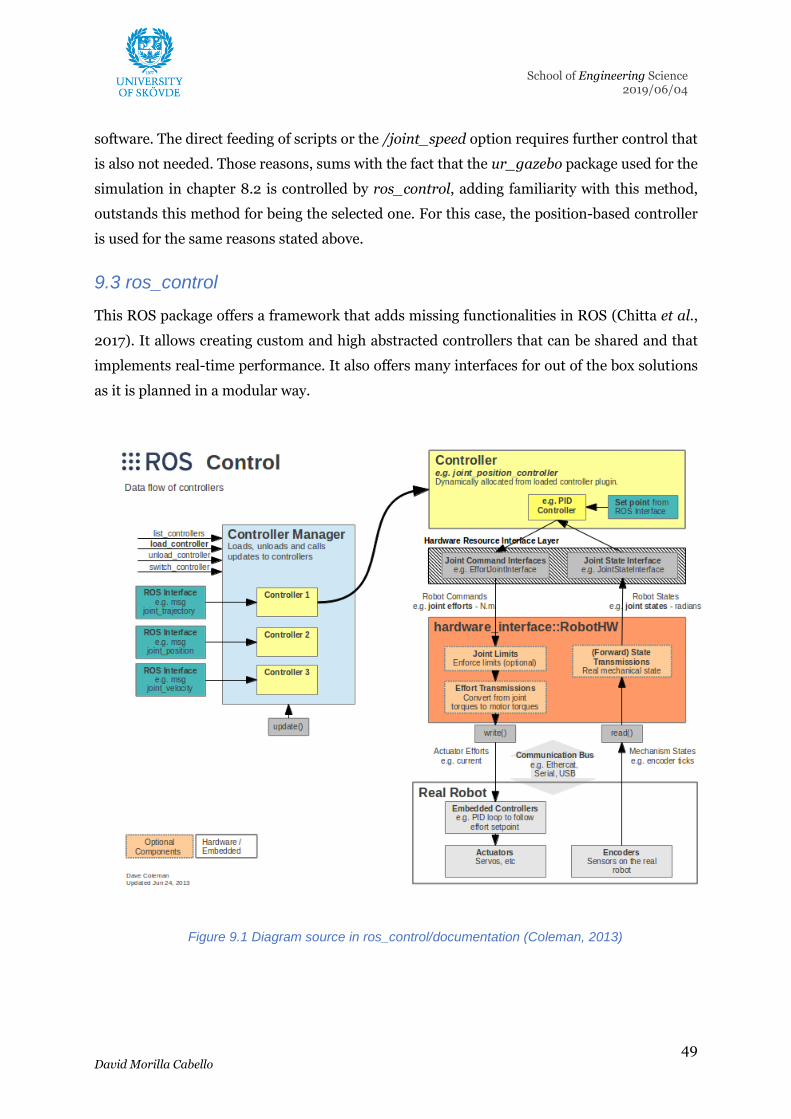
49 David Morilla Cabello
School of Engineering Science 2019/06/04
software. The direct feeding of scripts or the /joint_speed option requires further control that
is also not needed. Those reasons, sums with the fact that the ur_gazebo package used for the
simulation in chapter 8.2 is controlled by ros_control, adding familiarity with this method,
outstands this method for being the selected one. For this case, the position-based controller
is used for the same reasons stated above.
9.3 ros_control
This ROS package offers a framework that adds missing functionalities in ROS (Chitta et al.,
2017). It allows creating custom and high abstracted controllers that can be shared and that
implements real-time performance. It also offers many interfaces for out of the box solutions
as it is planned in a modular way.
Figure 9.1 Diagram source in ros_control/documentation (Coleman, 2013)
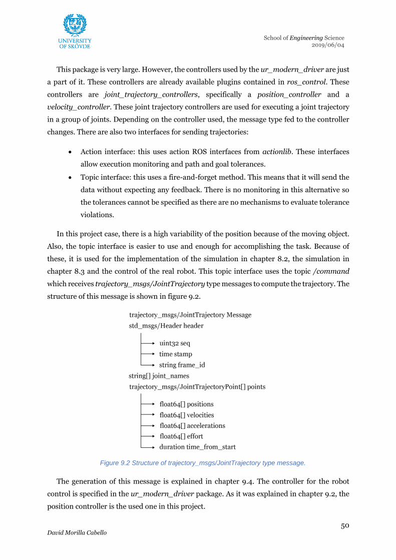
50 David Morilla Cabello
School of Engineering Science 2019/06/04
This package is very large. However, the controllers used by the ur_modern_driver are just
a part of it. These controllers are already available plugins contained in ros_control. These
controllers are joint_trajectory_controllers, specifically a position_controller and a
velocity_controller. These joint trajectory controllers are used for executing a joint trajectory
in a group of joints. Depending on the controller used, the message type fed to the controller
changes. There are also two interfaces for sending trajectories:
• Action interface: this uses action ROS interfaces from actionlib. These interfaces
allow execution monitoring and path and goal tolerances.
• Topic interface: this uses a fire-and-forget method. This means that it will send the
data without expecting any feedback. There is no monitoring in this alternative so
the tolerances cannot be specified as there are no mechanisms to evaluate tolerance
violations.
In this project case, there is a high variability of the position because of the moving object.
Also, the topic interface is easier to use and enough for accomplishing the task. Because of
these, it is used for the implementation of the simulation in chapter 8.2, the simulation in
chapter 8.3 and the control of the real robot. This topic interface uses the topic /command
which receives trajectory_msgs/JointTrajectory type messages to compute the trajectory. The
structure of this message is shown in figure 9.2.
Figure 9.2 Structure of trajectory_msgs/JointTrajectory type message.
The generation of this message is explained in chapter 9.4. The controller for the robot
control is specified in the ur_modern_driver package. As it was explained in chapter 9.2, the
position controller is the used one in this project.

51 David Morilla Cabello
School of Engineering Science 2019/06/04
9.4 Interface between MATLAB and ROS
In addition to the tools mentioned in chapter 7, the Robotic System Toolbox provides an
interface with ROS. There are many MATLAB functions and Simulink blocks for this. This
project implementation is centred on the use of the publish and subscribe block. As the name
indicates, the publish block is used to send messages to a ROS network. For this, the topic and
the message type are indicated. For code generation, the length of the publishing queue must
be selected too. The subscribe block is used for receiving messages from a ROS network. The
topic and message type are also selected. In this case, the callback queue is to be specified for
code generation.
The way of managing ROS messages in MATLAB and Simulink is using structs objects. In
MATLAB, the struct object corresponds to the equivalent well-known type in other
programming languages. However, in Simulink, structs are treated like signals in buffers. This
makes difficult the management of complex messages. In order to create a ROS message in
Simulink, a blank message of the desired type has to be created. Then, the fields of the message
can be filled using the bus assignment block. This method works for simple messages at least.
When the message enlarges its complexity, a MATLAB function needs to be used in order to
fill the created message or read the received messages.
Two important things should be remarked. Besides managing the struct of the message with
the function, if the output of those functions is ROS messages, they need to be manually
specified instead of inherited. This is done in the Ports and Data Manager setup of the MATLAB
function block. The type of output must also be manually created using the function
robotics.ros.createSimulinkBus(gcs). This function is executed in the initFcn callback of the
model and it automatically creates the needed bus types in the MATLAB workspace for the
Simulink model. The overall model is shown in figure 9.3.
Figure 9.3 ROS Interface System model.
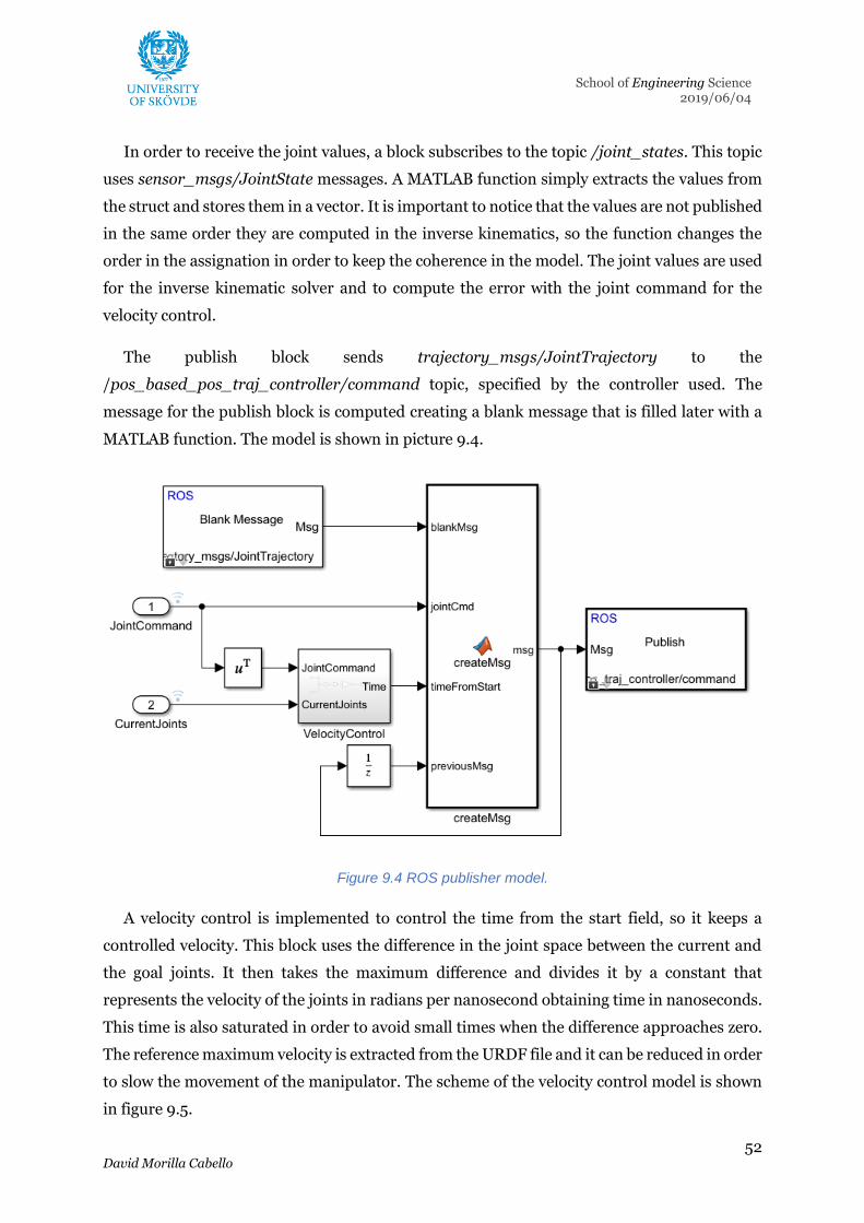
52 David Morilla Cabello
School of Engineering Science 2019/06/04
In order to receive the joint values, a block subscribes to the topic /joint_states. This topic
uses sensor_msgs/JointState messages. A MATLAB function simply extracts the values from
the struct and stores them in a vector. It is important to notice that the values are not published
in the same order they are computed in the inverse kinematics, so the function changes the
order in the assignation in order to keep the coherence in the model. The joint values are used
for the inverse kinematic solver and to compute the error with the joint command for the
velocity control.
The publish block sends trajectory_msgs/JointTrajectory to the
/pos_based_pos_traj_controller/command topic, specified by the controller used. The
message for the publish block is computed creating a blank message that is filled later with a
MATLAB function. The model is shown in picture 9.4.
Figure 9.4 ROS publisher model.
A velocity control is implemented to control the time from the start field, so it keeps a
controlled velocity. This block uses the difference in the joint space between the current and
the goal joints. It then takes the maximum difference and divides it by a constant that
represents the velocity of the joints in radians per nanosecond obtaining time in nanoseconds.
This time is also saturated in order to avoid small times when the difference approaches zero.
The reference maximum velocity is extracted from the URDF file and it can be reduced in order
to slow the movement of the manipulator. The scheme of the velocity control model is shown
in figure 9.5.

53 David Morilla Cabello
School of Engineering Science 2019/06/04
Figure 9.5 Velocity control model.
The inputs for the MATLAB function that creates the ROS message are all the necessary
data to fill the message (figure 9.2). This data is:
• The blank message to fill of the needed type.
• The joint command, as a vector of values for each joint, just one target is selected in
the trajectory. It means that this approach does not use any trajectory generation,
just an end target command. In case that a trajectory was generated, this vector
would have more than one value per joint.
• The time from the start of the trajectory when the goal has to be reached. This time
is computed by the velocity control.
• The previous message is also received in order to change the seq field increasing the
previous number by one.
The function fills all the necessary fields of the message structure exposed in figure 9.2.
To this struct, fields for CurrentLength are included in Simulink and must be manually
assigned in order to convert the message from a Simulink bus to a ROS message. In this
case, the length of the string and joint values are always the same as the number of joints
is not going to change. The array for joint names is fixed and defined inside the MATLAB
function. The seq field for the header is computed using the previous message seq
number plus one. Then, a for loop is used to assign the name of the joints in the data
field of joint names and its length in the data_sl_info field. Then, the joint commands
are stored in the first place of the points vector in the positions field. After the for loop,
the time from start is introduced in the nsec field for the first point of the trajectory.

54 David Morilla Cabello
School of Engineering Science 2019/06/04
Figure 9.6 ROS structure of the real robot control.
In this system, MATLAB sends the joint trajectory points to the
/pos_based_pos_traj_controller/command topic. Then, the controller and the driver send
the messages to the real robot. The /joint_states topic shows the joint values sent by the driver
from the robot. These values are received by MATLAB in order to perform the robot control.
This control method is the same that was used for the simulation in chapter 8.3 as it was
mentioned. The final setup in ROS is shown in figure 9.6. The single change is the Gazebo node
for the ur_modern_driver node. The network layout for controlling the real robot is shown in
figure 9.7.
Figure 9.7 Real robot network diagram.
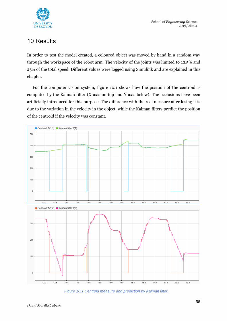
55 David Morilla Cabello
School of Engineering Science 2019/06/04
10 Results
In order to test the model created, a coloured object was moved by hand in a random way
through the workspace of the robot arm. The velocity of the joints was limited to 12.5% and
25% of the total speed. Different values were logged using Simulink and are explained in this
chapter.
For the computer vision system, figure 10.1 shows how the position of the centroid is
computed by the Kalman filter (X axis on top and Y axis below). The occlusions have been
artificially introduced for this purpose. The difference with the real measure after losing it is
due to the variation in the velocity in the object, while the Kalman filters predict the position
of the centroid if the velocity was constant.
Figure 10.1 Centroid measure and prediction by Kalman filter.

56 David Morilla Cabello
School of Engineering Science 2019/06/04
Figure 10.2 shows how the orientation changes from the image frame to the real-world
frame. It is also shown that the orientation is restricted to the first quadrant as the tool is
considered symmetrical and the orientation is thresholded to avoid sudden changes due to the
symmetry of the detected object. As the Kalman filter is not applied to the orientation, this is
supposed as constant while occlusion time and the value is not valid.
Figure 10.2 Orientation measure, correction and transform to the real-world frame.
Figure 10.3 shows the difference between the joint commands and the current joint states
for the joint that controls the pan of the arm (joint 1) in the 12.5% speed configurations. The
time difference between the goal and the current joint state is 0.76 s when the required joint
speed is an average of 2 rad/s. In figure 10.4, the same difference is shown for the 25% speed
configuration. In this case, the difference is 0.13 s when the required joint speed is an average
of 1 rad/s. Even if the difference depends on the velocity of the object and the exact set of
movements performed by the robot, the effect of the velocity limitation is clear. The capability
of following the object at a certain speed will depend on the maximum joint speed allowed in
the robot.

57 David Morilla Cabello
School of Engineering Science 2019/06/04
Figure 10.3 Difference between Joint command and Joint states for 12.5% speed configuration.
Figure 10.4 Difference between Joint command and Joint states for 25% speed configuration.
Figures 10.5 and 10.6 show how in both speed configurations the response is one step after
the command is sent. This means that the reaction of the robot is done at the sampling time of
the model, restricted by the frame rate of the camera (30 fps).

58 David Morilla Cabello
School of Engineering Science 2019/06/04
Figure 10.5 Time step since the first position is detected until the movement is started for 12.5%
speed configuration.

59 David Morilla Cabello
School of Engineering Science 2019/06/04
Figure 10.6 Time step since the first position is detected until the movement is started for 25%
speed configuration.
60 David Morilla Cabello
School of Engineering Science 2019/06/04
11 Discussion
The research process showed the best solutions for an out of the box implementation of
computer vision-based control of a robot arm. Following these criteria:
• Using already existing tools.
• Analysing the popularity of the options.
• Assuming that there is no previous experience in different programming languages.
The most feasible solutions to solve the problems are:
• Using MATLAB and/or Simulink interfacing with ROS.
• Using OpenCV based on Python or C++ directly in ROS.
Both approaches have clear advantages against current industry-used solutions as
explained in chapter 4.1.2. The first is flexibility in the designing and prototyping process. With
a wide variety of tools and implemented functionalities, different approaches can be easily
compared. The second is the velocity in the implementation. With appropriate knowledge of
the fields involved and the implemented functions, the solution for visual based control can be
achieved in a short time. The last advantage is the independence of the robot manufacturers
and third-party automation companies. As the solution is mainly apart from the robot
manufacturer software and is easy to implement, this allows working without incurring in time
or money expenses.
However, there are disadvantages to the current industry approach. The first is the necessity
of knowledge in many disciplines, while a purchased solution avoids a complex understanding
of the problem. The second is the support offered by those companies during all the life-cycle
of the product. Finally, the experience of those companies tends to be higher than the
experience of a single programmer as they are mainly focused on solving these tasks. This
factor will get a more robust solution to the problem.
Regarding the implementation, even if the MATLAB approach was used. The second
approach seems more appealing for performance and a real implementation task. However,
both approaches can be complementary to each other. MATLAB is normally used as a
prototyping software, thanks to its already built in tools, functions, and interfaces. However,
the licenses can be expensive for the payback, limiting its use to research or educational
61 David Morilla Cabello
School of Engineering Science 2019/06/04
institutions. Once the system is sketched, it can be ported to different software such as the
OpenCV library. One thing to remark is the similarity between MATLAB scripting and OpenCV
libraries for computer vision. However, using OpenCV would require more work from scratch
and additional research to this project in order to control the robot in ROS as a substitute for
the Robot Control System in MATLAB.
Some direct improvements could be applied to the result of the implementation. The
tracking velocity and reaction are estimated in the joint space. In order to acquire an exact
measurement in Cartesian space, velocity control for the TCP (instead of joints) and the
correspondent computation of the sensed velocity should be implemented using the Jacobian
Matrix. As the limitation of the model is the sample time of the camera, it is the bottleneck of
the system. In order to improve efficiency, the camera should be changed for a faster one.
12. Conclusion
The research in computer vision alternatives shows many available options to implement a
generic system with available software. These alternatives should be compared depending on
the user or specific interests in the project. All of them include basic requirements in order to
implement a whole visual servoing system. However, because of the popularity and
development, OpenCV and MATLAB are the most used software. Regarding the robot control,
there are also many alternatives to take into account in order to implement a system. The
research shows how there are existing options to control a UR3 manipulator, apart from the
provided basic software by the manufacturer, that allows more flexibility and complexity in the
control. These approaches involve a direct connection to the controller by a custom program
or using ROS. As a final conclusion, the research shows, not only that it is possible to
implement complex tasks based on computer vision in a robot manipulator but also, there are
many possible approaches. The selection of which method to use will depend on the specific
project but as an overall, they allow to implement generic solutions to a wide set of problems.
The implementation process also contributed to the study of the state of the art in software,
current problems and future needs of the study fields involved in the project. The developing
state of ROS suggests that there is a tendency for its future settlement in the automation
industry. Many robot manufacturers such as ABB or Universal Robots are collaborating with
its progress. MATLAB and OpenCV are also growing supported by their large user
communities. The implementation shows a satisfactory result with a good tracking speed
reaction and performance. The centroid and orientation are tracked with great accuracy using
a simple camera and a basic Kalman filter. The control of the robot also provides a good and
62 David Morilla Cabello
School of Engineering Science 2019/06/04
fast response to the tracking. It must be said that the fact that the package ur_modern_driver
is already created eased the implementation of the project and its result. In the case of other
robot manufacturers, the alternatives should be studied, and it could be more difficult to
integrate the robot hardware in the system.
This project covers a basic approach to a vast set of problems that can be solved in a more
efficient way. Some of these improvements are suggested here as future work:
• Include the grasping task of the object detected.
• Generate code in C++ from the Simulink model in order to improve the
performance.
• Create different controls for the robot in MATLAB as a velocity-based control using
the Jacobian Matrix or an effort-based control.
• Implement a computer vision system based on RGB-D cameras in order to improve
the 3D recognition.
• Include an eye-in-hand approach to get additional and more accurate information.
• Improve the connection to the robot using MoveIt! for real-time collision avoidance.
• Improve the controller and driver used.
• Create an interface between MATLAB and the robot without using ROS or port all
the system to the OpenCV library to reduce the variety of software used.
To conclude, the research and implementation processes show a blooming of improvements
and investigation in this area, providing new software, algorithms and tools. The system
designed mainly uses already created tools that allow huge flexibility and shows a decent
performance with a short time of implementation. This proves that better and more complex
systems can be implemented using the statements of this thesis.
It should also be noted the enlargement of personal knowledge and understanding that I
have acquired through this project. Computer vision, robot control, ROS systems, network
connections, or robot simulation are some new fields I was not familiar with. Disciplines that
are currently in the centre of the robotics research world and, along with the rising tendency
of open source progress, need the collaboration from many researchers as possible.
63 David Morilla Cabello
School of Engineering Science 2019/06/04
References
ABB ROBOTICS (2018) Conveyor tracking module. [Online]. Available from: https://library.e.abb.com/public/1c8cb39c0b8b40e585901d487eac10a1/Conveyor-Tracking-Module-CTM-presentation-rev.A-9AKK107046A7025.pdf [Accessed: 20 May 2019].
Acciona (n.d.) What is sustainability? | Sustainability for all. [Online]. Available from: https://www.activesustainability.com/sustainable-development/what-is-sustainability/ [Accessed: 3 May 2019].
Adelson, E.H., Anderson, C.H., Bergen, J.R., Burt, P.J., et al. (1984) Pyramid methods in image processing. [Online]. p.10. Available from: https://www.researchgate.net/profile/Joan_Ogden/publication/246727904_Pyramid_Methods_in_Image_Processing/links/544006600cf21227a11ba140/Pyramid-Methods-in-Image-Processing.pdf.
Agin, G. J. (1979) Real time control of a robot with a mobile camera.
Andersen, T.T. (2015) Optimizing the Universal Robots ROS driver. [Online]. p.36. Available from: http://orbit.dtu.dk/files/117833332/Universal_Robot_report.pdf.
Andersen, T.T. (2019) ROS driver for CB1, CB2 and CB3+ controllers with UR3, UR5 or UR10 robots from Universal Robots: ros-industrial/ur_modern_driver. [Online]. ROS-Industrial. Available from: https://github.com/ros-industrial/ur_modern_driver [Accessed: 5 May 2019].
Anon (2014) Gazebo. [Online]. 2014. gazebosim.org. Available from: http://gazebosim.org/ [Accessed: 3 May 2019].
Anon (2018) wiki.ros.org. [Online]. 2018. Documentation - ROS Wiki. Available from: http://wiki.ros.org/ [Accessed: 3 May 2019].
Balaji, S.R. & Karthikeyan, S. (2017) A survey on moving object tracking using image processing. In: 2017 11th International Conference on Intelligent Systems and Control (ISCO). [Online]. January 2017 pp. 469–474. Available from: doi:10.1109/ISCO.2017.7856037.
Barron, J.L., Fleet, D.J. & Beauchemin, S.S. (1994) Performance of optical flow techniques. International journal of computer vision. 12 (1), 43–77.
Ben-Ari, M. & Mondada, F. (2018) Kinematics of a Robotic Manipulator. In: Mordechai Ben-Ari & Francesco Mondada (eds.). Elements of Robotics. [Online]. Cham, Springer International Publishing. pp. 267–291. Available from: doi:10.1007/978-3-319-62533-1_16 [Accessed: 13 May 2019].
Bradski, G.R. & Kaehler, A. (2011) Learning OpenCV: computer vision with the OpenCV library. Software that sees. 1. ed., [Nachdr.]. Beijing, O’Reilly.
Canali, C., Cannella, F., Chen, F., Sofia, G., et al. (2014) An automatic assembly parts detection and grasping system for industrial manufacturing. In: 2014 IEEE International Conference on Automation Science and Engineering (CASE). [Online]. August 2014 pp. 215–220. Available from: doi:10.1109/CoASE.2014.6899329.

64 David Morilla Cabello
School of Engineering Science 2019/06/04
Chaumette, F. & Hutchinson, S. (2006) Visual servo control. I. Basic approaches. IEEE Robotics Automation Magazine. [Online] 13 (4), 82–90. Available from: doi:10.1109/MRA.2006.250573.
Chaumette, F. & Hutchinson, S. (2007) Visual servo control. II. Advanced approaches [Tutorial]. IEEE Robotics Automation Magazine. [Online] 14 (1), 109–118. Available from: doi:10.1109/MRA.2007.339609.
Chitta, S., Marder-Eppstein, E., Meeussen, W., Pradeep, V., et al. (2017) ros_control: A generic and simple control framework for ROS. The Journal of Open Source Software. [Online] 2 (20), 456. Available from: doi:10.21105/joss.00456.
Cigliano, P., Lippiello, V., Ruggiero, F. & Siciliano, B. (2015) Robotic Ball Catching with an Eye-in-Hand Single-Camera System. IEEE Transactions on Control Systems Technology. [Online] 23 (5), 1657–1671. Available from: doi:10.1109/TCST.2014.2380175.
Coleman, D. (2013) wiki.ros.org/ros_control. [Online]. 2013. wiki.ros.org/ros_control. Available from: http://wiki.ros.org/ros_control.
Corke, P. (2017) QUT Robot Academy. [Online]. 2017. Available from: https://robotacademy.net.au/ [Accessed: 3 May 2019].
El-Sherbiny, A., A. Elhosseini, M. & Y. Haikal, A. (2017) A comparative study of soft computing methods to solve inverse kinematics problem. Ain Shams Engineering Journal. [Online] 9. Available from: doi:10.1016/j.asej.2017.08.001.
Engell-Nørregard, M. (2007) Inverse Kinematics The state of the art. University of Copenhagen, Denmark, graduate project. 1–23.
Frese, U., Bauml, B., Haidacher, S., Schreiber, G., et al. (2001) Off-the-shelf vision for a robotic ball catcher. In: Proceedings 2001 IEEE/RSJ International Conference on Intelligent Robots and Systems. Expanding the Societal Role of Robotics in the the Next Millennium (Cat. No.01CH37180). [Online]. October 2001 pp. 1623–1629 vol.3. Available from: doi:10.1109/IROS.2001.977211.
Golz, J. & Biesenbach, R. (2015) Implementation of an autonomous chess playing industrial robot. In: 2015 16th International Conference on Research and Education in Mechatronics (REM). [Online]. November 2015 pp. 53–56. Available from: doi:10.1109/REM.2015.7380373.
Gornea, D., Popescu, D., Stamatescu, G. & Fratila, R. (2014) Mono-camera robotic system for tracking moving objects. In: 2014 9th IEEE Conference on Industrial Electronics and Applications. [Online]. June 2014 pp. 1820–1825. Available from: doi:10.1109/ICIEA.2014.6931463.
Horn, B.K. & Schunck, B.G. (1981) Determining optical flow. Artificial intelligence. 17 (1–3), 185–203.
Husain, F., Colomé, A., Dellen, B., Alenyà, G., et al. (2014) Realtime tracking and grasping of a moving object from range video. In: 2014 IEEE International Conference on Robotics and Automation (ICRA). [Online]. May 2014 pp. 2617–2622. Available from: doi:10.1109/ICRA.2014.6907234.

65 David Morilla Cabello
School of Engineering Science 2019/06/04
Hwang, K., Lee, J. & Jiang, W. (2017) Intelligent image base visual servoing controller for robot arm. In: 2017 International Conference on Advanced Robotics and Intelligent Systems (ARIS). [Online]. September 2017 pp. 33–34. Available from: doi:10.1109/ARIS.2017.8297178.
International Federation of Robotics (2018) Executive Summary World Robotics 2018 Industrial Robots.p.10.
International Organization for Standardization (2012) ISO 8373:2012(en), Robots and robotic devices — Vocabulary. [Online]. 2012. Available from: https://www.iso.org/obp/ui/#iso:std:iso:8373:ed-2:v1:en [Accessed: 3 May 2019].
Kalman, R.E. (1960) A new approach to linear filtering and prediction problems. Journal of basic Engineering. 82 (1), 35–45.
Klette, R. (2014) Concise computer vision. Springer.
KUKA (n.d.) Application software. [Online]. KUKA AG. Available from: https://www.kuka.com/en-se/products/robotics-systems/software/application-software [Accessed: 21 May 2019].
Kurry, A. (2011) Sustainable Development. [Online]. 2011. Available from: https://eportfolios.macaulay.cuny.edu/akurry/2011/12/21/sustainable-development/ [Accessed: 3 May 2019].
Kutzer, M. (2019) Contribute to kutzer/URToolbox development by creating an account on GitHub. [Online]. Available from: https://github.com/kutzer/URToolbox [Accessed: 5 May 2019].
Kwon, J., Lee, H.S., Park, F.C. & Lee, K.M. (2014) A Geometric Particle Filter for Template-Based Visual Tracking. IEEE Transactions on Pattern Analysis and Machine Intelligence. [Online] 36 (4), 625–643. Available from: doi:10.1109/TPAMI.2013.170.
Kwon, J., Lee, K.M. & Park, F.C. (2009) Visual tracking via geometric particle filtering on the affine group with optimal importance functions. In: 2009 IEEE Conference on Computer Vision and Pattern Recognition. [Online]. June 2009 pp. 991–998. Available from: doi:10.1109/CVPR.2009.5206501.
Lucas, B.D. & Kanade, T. (1981) An iterative image registration technique with an application to stereo vision.
Mao, Y., Lu, Q. & Xu, Q. (2018) Visual Servoing Control Based on EGM Interface of an ABB Robot. In: 2018 Chinese Automation Congress (CAC). [Online]. November 2018 pp. 3260–3264. Available from: doi:10.1109/CAC.2018.8623638.
MathWorks (n.d.b) Kalman Filter. [Online]. n.d.b. Design and use Kalman filters in MATLAB and Simulink. Available from: https://www.mathworks.com/discovery/kalman-filter.html [Accessed: 21 May 2019].
MathWorks (n.d.a) What Is Camera Calibration? - MATLAB & Simulink - MathWorks Nordic. [Online]. n.d.a. Available from: https://se.mathworks.com/help/vision/ug/camera-calibration.html [Accessed: 6 May 2019].

66 David Morilla Cabello
School of Engineering Science 2019/06/04
Matuska, S., Hudec, R. & Benco, M. (2012) The comparison of CPU time consumption for image processing algorithm in Matlab and OpenCV. In: 2012 ELEKTRO. [Online]. May 2012 pp. 75–78. Available from: doi:10.1109/ELEKTRO.2012.6225575.
McAndrew, A. (2004) An introduction to digital image processing with matlab notes for scm2511 image processing. School of Computer Science and Mathematics, Victoria University of Technology. 264 (1).
Mekki, H. & Kaaniche, K. (2016) Adaptive 2D visual servoïng using variable structure neural networks. In: 2016 13th International Multi-Conference on Systems, Signals Devices (SSD). [Online]. March 2016 pp. 494–498. Available from: doi:10.1109/SSD.2016.7473711.
Montúfar, P., Salazar, H., Aguilar, W., Segura, L., et al. (2017) Kalman filter implementation in a working cell to classify parts that are in motion. In: 2017 CHILEAN Conference on Electrical, Electronics Engineering, Information and Communication Technologies (CHILECON). [Online]. October 2017 pp. 1–7. Available from: doi:10.1109/CHILECON.2017.8229682.
Nnaji, B.O. (1993) Google-Books-ID: poAIavAqj68C. Theory of Automatic Robot Assembly and Programming. Springer Science & Business Media.
Nouzil, I., Raza, A. & Pervaiz, S. (2017) Social aspects of automation: Some critical insights. In: IOP Conference Series: Materials Science and Engineering. 2017 IOP Publishing. p. 012020.
Nubiola, A. (2015) The future of robot off-line programming. CoRo Blog. [Online]. Available from: https://coro.etsmtl.ca/blog/?p=529 [Accessed: 3 May 2019].
Oates, B.J. (2005) Researching information systems and computing. Sage.
Papert, S.A. (1966) The summer vision project.
Park, and F.C. (2008) Visual tracking via particle filtering on the affine group. In: 2008 International Conference on Information and Automation. [Online]. June 2008 pp. 997–1002. Available from: doi:10.1109/ICINFA.2008.4608144.
Pochyly, A., Kubela, T., Singule, V. & Čihák, P. (2017) Robotic bin-picking system based on a revolving vision system. In: 2017 19th International Conference on Electrical Drives and Power Electronics (EDPE). [Online]. October 2017 pp. 347–352. Available from: doi:10.1109/EDPE.2017.8123228.
Reddy, R. & Nagaraja, S.R. (2014) Integration of robotic arm with vision system. In: 2014 IEEE International Conference on Computational Intelligence and Computing Research. [Online]. December 2014 pp. 1–5. Available from: doi:10.1109/ICCIC.2014.7238302.
Ribnick, E., Atev, S., Papanikolopoulos, N., Masoud, O., et al. (2007) Detection of thrown objects in indoor and outdoor scenes. In: 2007 IEEE/RSJ International Conference on Intelligent Robots and Systems. [Online]. October 2007 pp. 979–984. Available from: doi:10.1109/IROS.2007.4398962.
Roshni, N. & Kumar, T.K.S. (2017) Pick and place robot using the centre of gravity value of the moving object. In: 2017 IEEE International Conference on Intelligent Techniques in
67 David Morilla Cabello
School of Engineering Science 2019/06/04
Control, Optimization and Signal Processing (INCOS). [Online]. March 2017 pp. 1–5. Available from: doi:10.1109/ITCOSP.2017.8303079.
Shaun Edwards & Felix Messmer (2019) ROS-Industrial universal robot meta-package (http://wiki.ros.org/universal_robot): ros-industrial/universal_robot. [Online]. ROS-Industrial. Available from: https://github.com/ros-industrial/universal_robot [Accessed: 3 May 2019].
Siradjuddin, I., Behera, L., McGinnity, T.M. & Coleman, S. (2014) Image-Based Visual Servoing of a 7-DOF Robot Manipulator Using an Adaptive Distributed Fuzzy PD Controller. IEEE/ASME Transactions on Mechatronics. [Online] 19 (2), 512–523. Available from: doi:10.1109/TMECH.2013.2245337.
Turabian, K.L. (2007) A Manual for Writers of Research Papers, Theses, and Dissertations: Chicago Style for Students and Researchers (Chicago Guides to Writing, Editing, and Publishing). and publishing. 7th ed. Chicago: University of Chicago Press.
Universal Robots (n.d.a) UR+ solutions | Everything you need to customize your UR robot arm. [Online]. n.d.a. UR+ Solutions. Available from: https://www.universal-robots.com/plus/ [Accessed: 21 May 2019].
Universal Robots (n.d.b) UR Download | Support Site | Universal Robots. [Online]. n.d.b. Available from: https://www.universal-robots.com/download/ [Accessed: 5 May 2019].
Universal Robots Support (n.d.) Remote Control Via TCP/IP - 16496. [Online]. Remote Control Via TCP/IP - 16496. Available from: https://www.universal-robots.com/how-tos-and-faqs/how-to/ur-how-tos/remote-control-via-tcpip-16496/ [Accessed: 14 May 2019].
Wang, L., Wang, Z., Yu, H., Ha, H., et al. (2015) Vision based robot for recognizing and grasping fast moving conveyor products. In: 2015 15th International Conference on Control, Automation and Systems (ICCAS). [Online]. October 2015 pp. 1211–1215. Available from: doi:10.1109/ICCAS.2015.7364813.
Zacobria (n.d.) Introduction to Universal-Robots Script Programming | UR Forum-Help-Q&A. [Online]. Available from: https://www.zacobria.com/universal-robots-knowledge-base-tech-support-forum-hints-tips/universal-robots-script-programming/ [Accessed: 5 May 2019].
Zhang, K., Zhang, L., Yang, M.-H. & Zhang, D. (2013) Fast Tracking via Spatio-Temporal Context Learning. arXiv:1311.1939 [cs]. [Online] Available from: http://arxiv.org/abs/1311.1939 [Accessed: 6 March 2019].
Zhang, Y., Li, L., Ripperger, M., Nicho, J., et al. (2018) Gilbreth: A Conveyor-Belt Based Pick-and-Sort Industrial Robotics Application. In: 2018 Second IEEE International Conference on Robotic Computing (IRC). [Online]. January 2018 pp. 17–24. Available from: doi:10.1109/IRC.2018.00012.
Zhang, Z. (2000) A flexible new technique for camera calibration. IEEE Transactions on Pattern Analysis and Machine Intelligence. [Online] 22 (11), 1330–1334. Available from: doi:10.1109/34.888718.

68 David Morilla Cabello
School of Engineering Science 2019/06/04
Zhao, Z., Huang, P. & Chen, L. (2017) Visual tracking and grasping of moving objects and its application to an industrial robot. In: 2017 IEEE International Conference on Real-time Computing and Robotics (RCAR). [Online]. July 2017 pp. 555–560. Available from: doi:10.1109/RCAR.2017.8311921.


![Industrial Robots Auto Saved]](https://img.dokumen.tips/doc/110x75/577d25ce1a28ab4e1e9f9d17/industrial-robots-auto-saved.jpg)