- VISION-ASSISTED ROBOT KINEMATIC ERROR ES'MMATION:

PRINCIPLE AND APPLICATION

Weidong Tang

A thesis submitted to the Department of Mechanical Engineering

in confodty with the requirernents

for the degree of Master of Scicnce (Engineering)

QueenYs University

Kingston, Ontario, Canada

Jdy, 2001

Copyright 8 Weidong Tang, 2001

National Cibrary 1*1 ,canada Bibliothèque nationale du Canada

* .. and . .. e t = Services B i o g r a p h i q u e s 395 Wellington Street 305, rue Wellington Ottawa ON KfA ON4 ôüawa ON K 1 A W Canada Canada

The author has granteci a non- exclusive licence allowing the National Li* of Canada to reproduce, loan, disîriiute or sel1 copies of this thesis in microform, paper or electronic formats.

The author retains ownership of the copyright in this thesis. Neither the thesis nor substantial extracts fkom it may be printed or otherwise reproduced without the author's pefmissioa.

L'auteur a accordé une licence non exclusive pemettant à la Bibliothèque nationale du Canada de reproduire, prêter, disûiiuer ou vendre des copies de cette thèse sous la forme de microfiche/nIm, de reproduction sar papier ou sur format électronique.

L'auteur conserve la propriété du droit d'auteur qni protège cette thèse. Ni la thèse ni des extraits substantiels de celle-ci ne doivent être imprimés ou autrement reproduits sans son atltorisa~~~.

Abstract

Vision-assisted robot kinematic error estimation is a robot vision application to find out

"where it is" of the robot or the surrounding objects. The vision system demonstrates the

observation of the robot motions in the image form, therefore it cm perfonn the

kinematic error estimation in the image featurr space and then transfomi it into 3D robot

space or camera space if necessary. The intemlated theones for the vision-assisteci

kinematic error estimation are discussed in this thesis.

A direct visual servo control system is an application of robot vision-assisted kinematic

emor estimation. The robot joint displacernent enors are measured in the image featurc

space by the vision system and sent to the joint controller. As a case study, a dirrct visual

servo control method for a SCARA type manipulator is discussed and the comsponding

simulations are presented in this thesis.

The direct visual servo control method could be an alternative control scheme when one

or more internd joint sensors fail. aie possible functions of a vision sysfem in the rhree-

level (servo level, interface level and supe~sor level) fadt tolerant system of a robot are

presented. Simulations demonstrated that a direct visuai servo control system codd be an

alternative controller to fulfill full recovery and partial recovery scherne at servo level.

This application shows a potential method to improve the fault tolerance capability of an

existing robot by employing a vision system.

Acknowledgements

Without the guidance and help of rny supervisor, Dr. Leila Notash, this work would never

have been completed. I would like to express my appreciation for her advice and

financial support throughout the course of my Master's program.

1 am also grateful for the financial support provided by the Department of Mechanical

Engineering, and the School of Graduate Studies and Research.

1 wish to thank ail the students in Robotics Lab of the Department of Mechanical

Engineering for the help on my research.

Finally, 1 hope this effort could be a linle repayment to my family and my fiiends for

their consistent encouragement. Because of hem, 1 had an enjoyable and unforgettable

time during rny study in Queen's University.

Tabfe of Contents

... ................................................................................................................... List of T a b l s viu

................................................................................................................... Nomenclature Ut

Chap ter 1 Introduction ..................................................................................................... 1

1.1 Robot Vision Application .................................................................................. 2 1.2 Vision-Assisted Kinematic Error Estimation ............................. .......................... 2 1.3 Direct Vision Servo Control Method .................................................................. 3 1.4 Improving Robot Fault Tolerance Performance .................................................. 4

2.1 Introduction ........................................................................................................ 6 2.2 Robot Vision Theory and Applications ......................... ..... .......................... ... 7

...................................................... ..... 2.2.1 Human Vision ........................................ 8 2.2.2 Machine Vision ........................................... 10 2.2.3 Robot Vision Application Mode1 .................................................................... 11

2.3 Image Formation and Camera Mode1 ............................................................... 13 2.3.1 Image Formation ............................ .. .......................................................... 13 2.3.2 Carnera Mode1 ................................................................................................. 16

2.3.2.1 Pinhole (Cenaal Perspective) Projective Mode1 .................................... 16 2.3.2.2 Orthogonal Frojective Mode1 .................................................................... 16 2.3.2.3 Affine Projective Mode1 ........................................................................... 17

2.3.3 Camera Placement .......................... ., ............................................................... 18 2.4 Image Features and Feature Extractor ............................................................. 20 2.4.1 Image Features ............................................. ...... ......................................... 20 2.4.2 Feature Extractor ............................................................................................. 24

2.5 Reconstruction, Interpretation and Decision .................................................. .. 26 2.5.1 Reconstxuction ...................................... ,, . . . . 27 2.5.2 Interpretation and Decision ................... ..... ........................................ 30 2.6 Robot Vision Application .......... .. ................................................................ 31

Chapter 5 Simulation of a Dùect Visual Servo Control Method for a Three-DOF SCARA Type Manipulator eeee.ee.......~........................................................... 96

........................................................................................................ 5.1 Introduction 96 ........................................................................ 5.2 Basic Parameters for the Models 97

............................................................................ 5.2.1 Parameters for Manipulator 97 ..................................................................... 5.2.2 Parameten for Projection Mode1 98

......................................................................... 5.2.3 Controi and Other Parameters 99 ....................................................................................... 5.3 Prescribed Trajec tories 99

................................................................................ 5.3.1 Known Joint Trajectory 100 .......................................................................... 5.3.2 Known Endpoint Trajectory 101

5.4 Simulation Program Flow Chart ................... .. ............................................. 101 ........................................................................................... 5.5 Simulation Results 104

5.5.1 Simulation Results with no Error Input ......................................................... 104 ....................................... 5.5.2 Simulation Results with Image Cooordinate Error 118

................... ................. 5.5.3 Simulation Results with Dynamic Disturbance ...... 127 5.5.4 Simulation Results with Link Length Error ................................................ 128 5.5.5 Simulation Results with Joint Velocity Lirnits ............................................. 129

.............................................. 5.5.6 Simulation Results with Torque/Force Limits 130 5.6 Summary .......................................................................................................... 135

...................................................................................................... 6.1 Introduction 137 ............................................................ 6.2 Application in Fault Tolerance S ystem 139

6.2.1 ServoLayer .............................................................................................. 141 6.2.2 Interface Layer ............................................................................................ 149

......................................................................................... 6.2.3 Supervisor Layer 152 6.3 Joint Position Measurement of a Puma Type Manipulator ....................... ..... 153

. . 7.1 Conclusions and Contributions ......................................................................... 159 7.2 Future Works ................................................................................................... 162

Vita ....................... .- ................................................................................................... 170

Figure 2.1 Figure 2.2 Figure 2.3 Figure 2.4 Figure 2.5 Figure 2.6 Figure 2.7 Figure 2.8 Figure 2.9 Figure 2.10 Figure 2.1 1 Figure 3.1 Figure 3.2 Figure 4.1 Figure 4.2 Figure 4.3 Figure 4.4

......................................................... Vision application procedure mode1 12 . . Pinhole projection mode1 ............................................................................. 16

....................................................................... Orthogonal projective mode1 17 Eye-to-hand camera placement .................................................................... 19 Eye-in-hand carnera placement .................................................................... 19 Potential features that can be processed by the image processing ............... 21 Reconstruction is the inverse mapping of projection ................................... 27 Position-based look-and-move(PBLM) mode1 .......................................... 34

................................................ Image-based look-and-move(IBLM) mode1 34 .................................................. Position-based visual servo(PBVS) model 36

Image-based visual servo(R3VS) mode1 .................................................... 36 Task description and observation with vision system ............................... .. 46 Transformation from camera frarne to image frame .................................. 51 SCARA robot (Resource: Adept Inc.). ........................................................ 77 Example of the-DOF SCARA type manipulator ..................... .. ............ 77 Overhead view of the example SCARA type robot ..................................... 85 Joint angles in robot space and camera space under scaied orthogonal

. . .................................................................................................................... projection 87 Figure 4.5 Side view of the third joint from the camera .............................................. 88

....................................... Figure 4.6 Joint PD controller with a known joint trajectory 92 Figure 4.7 A joint PD controller with known Cartesian trajectory . M applied to

. . ............................................................................ estimate the desired joint trajectory 93

Figure 4.8 A joint PD controller with known Cartesian trajectory . FK applied to estimate the real end effector trajectory . ................................... .................... 94

Figure 5.1 The Bow chart of the simulation program ............................................. 103 Figure 5.2-1 TRAJl with no enor input: (a) tmjectory of end point, (b) and (c)

............... trajectories of f i t and second joints, (d) to (f) joint displacernent emrs 106 Figure 5.2-2 M l with no error input: (a) to (c) joint velocity. (d) to (f) joint

............................................. acceleration, (g) to (i) joint forceltorque .. ......... 107 Figure 5.2-3 TRAJl with no e m r input: (a) trajectory of end point. (b) and (c)

trajectones of first and second joints. (d) to (f) joint displacement emrs . Step time = 0.08 ms ....................................................... 108

Figure 5.2-4 TRAJl with no error input: (a) to (c) joint velocity. (d) to (f) joint acceleration, (g) to (i) joint force/torque . Step time = 0.08 rns ................................ 109

Figure 5.2-5 TRkll with no e m r input: (a) to (c) joint velocity, (d) to (f) joint acceleration . (g) to (i) joint torqudforce . Image sampling e m r = 2rnm/pixel ........ 110

figtwe 5.2-6 TRkll with no fiction: f e> tmjeetexy ef end point, (b.> and (c) tnjectoriies of fint and second joints, (d) to ( f ) joint displacement e m n .................................... ... 11 1

Figure 5.3 TRkl2 with no error input: (a) tmjectory of end point, (b) and (c) trajectones ................................. of first and second joints, (d) to (f) joint displacement e r m . 112

Figure 5.4-1 TRAJ3 with no error input: (a) trajectory of end point, (b) and (c) .............. trajectories of fïrst and second joints. (d) to (f) joint displacement errors. 113

Figure 5.4-2 TRAJ3 with no error input &er adjusting the control parameters: (a) trajectory of end point, @) and (c) tmjectories of fint and second joints, (d) to (f)

............................................................... ...................... joint displacement errors. .. 1 14 Figure 5.5 TRAJ3 with no error input after adjusting the mass: (a) trajectory of end point,

(b) and (c) trajectories of f i t and second joints. (d) to ( f ) joint displacement errors

......................................................................................................................................... 115 Figure 5.6- 1 TRAJ3 with random image coordinate emr: (a) trajectory of end point, @)

......... and (c) trajectories of first and second joints, (d) to (f) joint displacemeni errors. 119 Figure 5.6-2 TRAJ3 with adjusted mass and random image coordinate enor: (a)

trajectory of end point, (b) and (c) trajectories of first and second joints. (d) to (f) joint displacement errors. ....................................................................................... 120

Figure 5.7-1 TRAJ3 with dynamic disturbance: (a) trajectory of end point, @) and (c) .............. trajectories of fmt and second joints, (d) to ( f ) joint displacement enors. 121

Figure 5.7-2 TRAJ3 with dynamic disturbance after adjusting the mas: (a) tmjectory of end point, (b) and (c) trajectories of first and second joints, (d) to (f) joint

................................................................................................ displacement enors. 122 Figure 5.8-1 TRAJ3 with iink length enors: (a) trajectory of end point, (b) and (c)

.............. trajectories of fint and second joints, (d) to (f) joint displacement emrs. 123 ................ Figure 5.8-2 TRAJ3 with link length emrs: coordinate e m n of 01 and 0 2 124

Figure 5.9-1 W 3 with link length enors after adjusting the mass: (a) trajectory of end point, @) and (c) trajectones of first and second joints, (d) to (f) joint displacement errors ......................................................................................................................... 125

Figure 5.9-2 TRAJ3 with link length errors a€ter adjusting the mass: coordinate emrs of 01 and 02 ................................................................................................................ 126

Figure 5.10 T M 3 with velocity limits: (a) tnjectory of end point, (b) and (c) trajectones ..................... of first and second joints, (d) to (f) joint displacement errors. ...... 132

Figure 5.1 1 - 1 TRAJ l with force limits: (a) trajectory of end point, (b) and (c) trajectones of fmt and second joints, (d) to ( f ) joint displacement emrs. ................................. 133

Figure 5.1 1-2 TRAJl with force limits after adjusting the control parameters (a) trajectory of end point, (b) and (c) trajectories of £kt and second joints, (d) to (f) joint displacernent emrs ....................... .... ........................................................ 134

Figure 6.1 Vision system in a robot fault tolerance system. ................................... 140

vii

Figure 6.2 Vision system in the seno layer of a fault tnierance mhat syset m. .. 142 Figure 6.3- 1 Scheme without full recovery: displacement tracking performance . The

sensor of the second joint is failed at 1.5 sec ........................................................... 145 Figure 6.3-2 Full recovery scheme: displacement tracking performance . The sensor of the

second joint is failed at 1.5 sec and replaced by the vision system immediately ..... 146 Figure 6.4-1 Scheme without partial recovery: velocity and force . The sensor of the

second joint is failed at 2.5 sec . The system cannot stop smoothly ......................... 147 Figure 6.4-2 Partial recovery scheme: velocity and force . The sensor of the second joint is

failed at 2.5 sec and replaced by the vision system ...................... .. ........................ 148 Figure 6.5 Traditional model-based robot failure anal ysis ......................................... 150 Figure 6.6 Vision-based robot failure andysis ............................................................ 151 Figure 6.7 Vision system in the supervisor layer of the fault tolerance system .......... 153 Figure6.8 PUMArobotwithvisionsystem ............................................................ 154

........................ Figure 6.9 The relationship between the iine segment and its image 155

List of Tables

Table 2.1 Three Ievels of Mm's vision mode1 .............................. ...,.. 11 Table 2.2 Cornparison of different visual control rnethods ............................................. 35 Table 3.1 Comparison of vision-assisted kinematic error estimation methods ............... 65 Table 4.1 D-H parameters of a the-DOF SCARA robot ............................................. 78 Table 5.1 D-H parameten of the example three-DOF rnanipulator ............................. 97

output torque andor force vector of joint actuator (in N m for torque

and N for force)

horizontal and verticai sampling intervals in an image

image coordinates of a point in an image

digital coordinates of an image point

digital coordinate of the center of the image plane

coordinates of the origin of the ith joint frame in base frame

depth from the centroid of the observed point set to the viewpoint

point-to-point tracking error

position error function (in m) and its denvative with respect to time

(in m / s )

Coulomb friction

viscous friction

dynamic term associated with fiction

focal iength of the camera

desired and actual image feature vectors

feature Jacobian matrix

proportionai gain vector (in Nmim for revolute joint and Nlm for

prismatic joint)

derivetive gain veetor fin N m drrtd for revoIute joint and N dm for

prismatic joint)

actual length and image length of a iine segment

inertia matrix

mass (in kg)

dynarnic term associated with the Coriolis force, centrifugai force

and gravity

position vector in 2D image space

position vector in 3D space (robot spacc or camaa space)

Tb..

AIS

CCD

D-H

DOF

FMEA

FTA

IBLM

IBVS

PBLM

PBVS

P D

PUMA

SCARA

TFS

transformation matrix from frarne a to frame b

estimated transformation matrix h m frarne a to frame b

joint force

joint velocity

Augmented Image Space

Charge Coupled Device

Denavi t-Hartenberg

Degree of Freedom

Failure Mode and Effect Analysis

Fault Tree Analysis

Image-Based Look-and-Move

Imaged-Based Visual Servo

Posi tion-Based Look-and-Move

Position-Based Visual Servo

Proportional and Denvative

Proportional. Integral and Derivative

hgrammable Universal Machine for Assembly

Selectively Cornpliant Aaiculated Robot Ann

Transformed Feature S pace

Desired Robot Trajectory #1 @fer to Section 5.3)

Desired Robot Trajectory #2 (refer to Section 5.3)

Desired Robot Trajectory #3 (refer to Section 5.3)

Chapter t

Introduction

The main objective of this project is to improve the performance (such as fault tolerant

capability) of an existing robot by equipping the robot with a vision system. For fault

tolerance, there are generally two tasks: detection of the failures and recovery h m the

failures.

In order to acheve the goal of this project, vision-assisted robot kinematic error

estimation is studied. The purpose of this study is to check the kinematic erron of each

joint of the robot with a suitable vision system. Combined with other advantages of a

vision system and the functions of other sensors, the vision system could become a good

failure inspecter. The vision-assisted robot kinematic error estimation can be applied in a

direct visual servo control method, which has been proposed for a SCARA type

manipulator in this thesis. This method mats the joint position error estimation in terms

of image coordinates as the control e m r signal, which is sent to the joint controller.

A direct visual servo conml system could become an alternative contmller when one or

more sensors fail. From the viewpoint of a fault tolerance theory, this system can play a

role at the servo level of the fault tolemce system of a robot. Further analysis can show

that a vision system can function at different levels of a three-layer fault tolerance

system. The advantage is that an existing robot can gain additional fault tolerant

capabilities without ciramatic structure changes by employing a vision system.

1.1 Robot Vkion Application

Vision technology has k e n a popular topic in mbot research laboratones for years.

Besides the studies on the human/animal vision with the goal of understanding the

operation of biological vision systems, more and more vision resemhers stress on

developing vision systems for the application in an industrial envuonment such as

navigation, and recognizing and tracking objects.

An acnial vision system could not perform the whole functions as weU as the eyes of a

human being do. However, robot vision technology provides a combination of flexibility,

adaptabili ty, precision, non-contact measurement and object recognition for robotics.

Generally, the vision system could answer two questions: what it is and where it is. Here

"it" refers to the observed object in the scenery. A robot vision system could answer both

questions, but often focuses on one of them.

The vision application model introduced in Figure 2.1 shows the information flow among

different function modules. The research on the corresponding theories and applications

will be àiscussed based on the structure of chis model.

1.2 Vision-Assisted Kinematic Error Estimation

Vision-assisted robot kinematic error estimation is a robot vision application ïo find out

"where it is" of the robot or the sumunding objects. The vision system demonstrates the

observation of the robot motion in the image form. Therefore, robot motion description

(expected and actual) c m be defined in the image space and then robot kinemah'c crms d

estimation can be completed in robot space. camera space or image space. Usually the

estimation results are represented in image featue space or msformed into thne

dimensional (3D) robot space or carnera space. However, in some cases the

transformation is not necessary if the required task motion and the actual motion cm be

both described in the image space.

Chapter 3 will present the theories of the vision-assisted Ianematic e m r estimation.

These theories discuss the following topics: transformation among world space, camera

space and image space; camera projection model; reconstruction from the image features;

etc. There are different vision-assisted kinematic e m r estimation methods depending on

the camera placement and the task description space. The different methods wül be

compared with each other. Feature Jacobian matrix, which refiects the relationship

between the feature space and 3D world space, will be presented case by case.

A direct visual servo control system is an application of the vision-assisted kinematic

error estimation. Currently most of the robot tasks are defined by the trajectory of the end

effector, so a vision system is often used to recover the position information of the robot

end effector and the objects around the robot. However, a direct joint position

measurement is necessary if a direct visual servo control system is requii.ed A diract

visual servo control method for a SCARA type manipulator will be discussed and

simdated in Chapters 4 and 5. The simulation results will show that the vision system

could meww the joint position dir;ectly in tenns of the images coordinates of the s@d

geometrical feature points of the robots, and it is feasible to form a visual servo control

system for a SCARA type manipulator with the joint position enor estimation in the

image feature space.

In Chapter 6 a method is discussed to show how to use a senes of line segments as the

features for rneasuring the joint positions of a PUMA type robot. This discussion shows

the flexibility of implementing the vision system for a specific robot. Analysis of the

structure of a robot can help the selection of the suitable features that will lead to a

successful vision application.

1.4 lmproving Robot Fault Tolerance Performance

Robots are being more frequently utilized in inaccessible or hazardous environments to

alleviate some of the risks involved in sending humans to perfom the tasks and to

decrease the respiring time and expense. It is h n g to be a more and more important

issue that a robot should have autonomous fault tolerance without requinng immediate

human intervention for every failure situation. A new robot can always gain fault

tolerance capability frorn the speaal considerations during the design procedure.

However for an existing robot it is quite difficult to improve its fault tolerance

performance wi thout changing its structure.

The discussion in Chapter 6 shows that a vision system can ffexibly and extensively

collect the information in the robot workspace and provide the possibility to improve the

4

fauh tohmce of en existittg robot. A vision system am @fornt di.ffepenk funcéhns in

different iayen (servo layer, interface layer and supervisor layer} of a robot fadt

tolerance system.

The direct visual servo convol system could be the basic module of the robot fault

tolerance system, which can allow the robot to continue perfonning its tasks or to

gracefully degrade if one of the joint sensors is failed. A vision system has the ability to

perform a nontontact measurement and to provide a broad view of the robot workspace

in world space. The results from the vision system could be compared with the

information obtained from other sensors or sources in order to point out the failure of the

joint movernent and supply more information for the rask manager to avoid unsafe

actions. More advantages of a vision system in a fauit tolerant robot are aiso discussed in

Chapter 6.

Chapter 2

Literature Review

2.f Introduction

Robot vision technology has become one of the most popular topics in robotics research.

Currently, vision sensors not only are experimental devices in the laboratones but have

also become standard components for many indusaial robots (such as welding, inspection

of automobile parts), space robots and housework robots, etc.

This chapter is a survey of the related robot vision theories and applications. The

following topics wiil be presented:

Basic vision theories: vision system can be considmd as an infoxmation-processing

model, which is the process of discovenng h m images what is present in the world and

where it is. Based on the different projective assurnptions and mathematical theories,

various vision models have been developed in recent years.

Image processing procedures: an image processiing procedure includes featwe

extraction and pattern recognition. Depending on the featms selected h m the image, a

lot of different methods could be applied. For robot vision applications, selected features

should be understood and detected relatively easily. Matching the comsponding feanires

in two or more images from the same scene is the most difncult part. Some abstract

feanires (such as resuits of wavelet transfomation) have been used in some applications.

Reconstruction approaches: the goal of reconstruction is to obtain information of

the observed o b j a from the image sequemes and rekabty to guide the action of &

robot or related rnachinery. The reconstruction can be in 3D or 2D image space. There is

no general reconstruction method. In order to obtain correct information about targets,

interpretation and decision procedures should be involved. In recent years, considerable

efforts have been devoted to object reconstruction based on image movement and

projective geometry.

Robot vision application: depending on the purpose of the vision system, there are

two kinds of robot vision applications. One is to find "what it is" in the scene. The other

is to find "where it is". Finding "what it is" helps robot to make some decisions for task

planning. A typical applicatiori is obstacle avoidance for mobile robots. Finding "whehen it

is" helps robot to meas= the position of the objects in the scene or the relative position

between objects and carneras. A typical application is visual servo control technology.

The contents of this chapter will be arranged as follows. Section 2.2 discusses the basic

theory and a robot vision application model. Section 2.3 discusses the image formation

and different camera model description. Section 2.4 discusses the image processing

technology. Section 25 intmduces reconstruction methods and necessary description aad

decision making procedure. Section 2.6 intmduces two kinds of robot vision applications

and stresses on the visual servo control technologies.

2.2 Robot Vision Theory and Applications

There are two groups of scientists working on vision. One group includes

neurophysiologists, ps ychophysicists and physicians, who are studying human/animal

vition with the g d of understanding the operation of biofogieitt visim eystem.

including their limitations and diversity. The other group includes cornputer scientists and

engineers doing research in machine vision with the purpose of developing vision

systems that are able to navigate, recognize, track objects and estimate their s p e d and

direction. The first group influences the design of vision systems by the second group. At

the sarne time. the second group helps the first group to mode1 biological vision 1461.

Robot vision is an application of machine vision in robotics. Machine vision simulates

some functions of human vision and therefore it is based on the research on biological

vision. Although some excellent human vision models are available, it is not easy to

apply these models to machine vision. In this section, the structure of robot vision

application procedure will be gi ven.

2.2.1 Human Vision

The efforts to understand how light signals are transuded into neural activity and how that

activity is transfonned through the neuro system has intrigued neurobiologists for many

years. Masland [63] has introduced the research status about the functions of the reha

For many years, the retina was known to be composed of five main classes of neurons.

Now it has become clear that the number of functional elements may be as high as 50.

Each functional element can process different information. Some translate static

information such as color, shape, etc. into human brain; some translate dynamic

information such as subtie changes due to the object movement relative to the

background. According to some researck* the &na has turo sets of n a c o s those that

establish a direct pathway from the source of light to the optic nerve and those that make

laterai connections. It is likely that the human vision system cm collect more information

in the scenery (not just shown on the picture taken by camera) and process them to obtain

a more accurate description of the observed object in the world.

Kondo and Ting [53] presented the main advanrages of the human binocular system:

O Eyes are sensitive to a slight change of brightness or color.

Eyes are able to acquire high-resolution images.

Eyes are able to detect motion parallac with a slight motion of the eyeball.

Brain is able to constnict 3D scenery by combining binocular-vision output with

various dues such as motion parallax and continuity of contours.

However, there is an interesting weakness in human vision system: the computation

speeds of individual neurons in the retina are about a million times slower than electronic

devices (but consume one ten-millionth as much power). They also operate with far less

precision than does a digital computer [6û]. This phenornenon highhghts that

Biological computation must be very different fkom the digital computer.

O Brain has a very different reconstruction model from that used in research.

Insects' vision indicates that they rnainly use selfmotion to sense distances to targets for

navigation and obstacle avoidance. Compared to human vision, insects have relatively

simple, but effective visual systems. This feature implies that robot vision might have

diverse functioaal models but might not necesad- be p e d ~

2.2.2 Machine Vision

Machine vision, which originated from photogrammi=try [64], is thought to have the

ability to sense, store and recover an image that matches the original space as closely as

possible. Photogrammetry concentrates on the recovering of position information of the

world. Based on the photogrammetry, machine vision technologies expanded into new

research areas such as object recognition.

M m [62) presented two questions, one or both of which should be answered by a typical

machine vision system:

What is presented in the world

Where it is

Furthemore, there are four basic questions that should be answered before setting up a

special machine vision system:

What kinds of images are required? This question concentrates on the camera

placement, viewpoint, illumination, etc.

What kinds of features should be found in the images? This question concentrates

on the distinctive characteristics of the objects with specid optical projection.

How to present the features? This question concentrates on the mathematical form

of the features obtained from the images.

How to recover the observed object using the feahires obtained from the images?

The above four questions are interrelated. For example, the selection of the features cm

influence the image processing and reconstruction rnethods.

Table 2.1 Three levels of Mm's vision model [62].

Computational Theory 1 Representation and Algorithm

What is the goal of the

computation?

W h y is it appropriate?

What is the logic of the

strategy by which it c a . be

carried out?

How can this computational

theory be implemented?

What is the representation

for the input and output?

What is the algorithm for the

transformation?

Hardware Irnplementation

How cm the algorithm

and representation be

realized physically?

M m (621 synthesized a vision model. This information processing model inciudes three

leveis as shown in Table 2.1. Marr pointed out that a machine vision system should

perfom two tasks to answer the above four questions:

Representing the information: this is the basis for decisions on how to treat the

observed results. At this step, the types of features and the way to represent the featurrs

should be decided.

Pmcessing the information: this analyzes the usefbl information extracted from the

image to show the various aspects of the world, such as beauty, shape and motion.

2.2.3 Robot Vision Application Mode1

Robot vision, which concentrates on pattern recognition, positioning, inspection and

modeling of objects, is the application of machine vision in robotics. With the

development of maFhins vision techndogy, more and mort robots are equipped with a

vision sensory system. In most of the robot applications, ody a partial description of the

scenery is necessary, which cm help the robot recognize special objects (marks) or

evaluate its movement accuracy relative to the environment.

According to the charactenstics of robot applications, a typical robot vision application

procedure is illustrated in Figure 2.1. Different parts of this model could be investigated

to produce various practical technologies suitable for different applications.

vision S8nSOC - feature

model extractor

Figure 2.1 Vision application procedure model.

The terminologies and concepts used in Figure 2.1 are explained as follows:

Objects: They are observed objects in 3D space. They are also caiied targets.

Images: They are results of the transformation h m 3 0 world space to 2D image

space. They cm be storeci on films or in cornputer memones.

Features: They are usefid image features extracted fiom a 2D image. Usually

they could be geometrical feahues as well as some abstract features.

Interpretation: It is a 3D mode1 description of the objects/targets. It is not the

teal original object but a partial descxiption of the obsenred ohject Sametimcs this

interpretation not only is incomplete, but also produces ambiguities.

O Vision sensor rnodel: It is a mathematical description of the individual vision

sensor. It cm redire the transformation fiom a 3D space to a 2D image space.

Feature extractor: It is a series of image processing methods to extract the useful

features from the images. It should be designed according to the applied features.

Reconstruction model: It is an algorithm for realizing the riansformation from

2D image space to 3D space. Theoretically, it is an inverse procedure of image formation.

Due to information loss during al1 of the previous processes and mathematical

limitations. the reconstruction model is often an independent model and very different

from the vision sensor model.

O Decision model: It is the method to analyze the results of interpretation, to obtain

reasonable information with physical meanings and to decide how to use the results.

2.3 lmage Formation and Camera Model

Image formation is a procedure, which transfers the 3D information into 2D image space.

Image formation has a strong dependency on the camera model (more generally it is

called vision model). In this section, basic image formation theories and three typical

camera models will be discussed.

2.3.1 lmage Formation

The images used in robot vision research are very different fkom the images on the retina

of a human king. The p w p l e of human vision is s t i l l a big question far hidogists even

though some cornplicated descriptions about the retina structure have been set up [63].

Presentiy there is no general vision mode1 for practical vision applications. Depending on

the individual application or research, different image formation techniques can be

selected. Usually only partial information cm be recorded and used from an image.

Physicaliy the image formation is a procedure to process the light flow from the scenmy

or objects and store hem on a special media, which can be film or computer memory.

Mathematically the image formation is a transformation h m a 3D description of the

observed objects into a 2D d e ~ ~ p t i o n .

M m [62] pointed out that the image charactexistics are influenced by many factors:

Geometry of the obsewed objects: this is the basis of an image. Especiaily in a

robot vision application, the geometry is a very important feature.

Reflectance of the visible surfaces: this influences the gray-level of the targets.

IIIumination of the scene: this influences the background of the image or

signdnoise ratio of the image.

Viewpoint: this decides the optic path from the object to the image plane.

For a vision application, charge coupled device (CCD) carnenis have been extmsively

used. CCD cameras can output elecaonic signals, which can be easily üansferred into

digital signals operated by a computer. Furthemore ail photosites are sampled

simultaneously when the photosite charge is transferred to the transport registm [II].

Active vision

Bajcsy [8] pointed out that human vision perception is not passive, but active. This

adaptation is crucial for survival in an uncertain environment. Active vision is the control

of the optics and the mechanical structure of cameras to simpiify the pmcessing of

cornputer vision. Active vision techniques such as active 3D sensors with stnictured

iighting [2] [92] [95] can highlight some features to facilitate the object recognition.

Bajcsy [8] presented two kinds of active vision methods:

Transmit electromagnetic radiation (e.g., radar, sonar) into the environment and

measure the ~flected signal by time-of-fhght sensors.

Employ a passive sensor in an active fashion, purposeNly changing the sensor's state

parameten according to sensing strategy.

Laser measurement s ys tem is an example measurement method that uses tirneof-flight

pnnciple. It is suitable for high accuracy meastuement between two points or two paral1el

planes. If multi dimensional or random directional measurements are quired, then a

high speed scanning mechanism is necessary. It is not easy to use a laser device to foIlow

a point with unpredicted movement. The cost of laser device is another concem.

Passive vision

In passive vision there is no special efforts on the f e a m s of the objects. The objects are

observed in natural iighting. A passive vision system is more suitable for robot

applications in unstructured environments such as space, undemater or missile tracking.

2A2 Camera Mode1

Based on the different projective assurnptions, three carnera models are setup as follows:

23.2.1 Pinhole (Central Perspective) Projective Model

Pinhole model is the most popular and traditional projective model. The center of the lens

is imaged as a point (pin-hole), through which light c m go through. Maybank [64]

introduced the basic principles of the pinhole projection.

3D Object Space

Figure 2.2 Pinhole projective model.

The image surface is taken to be a plane, but sphencal surface with a center at optical

center O shown in Figure 2.2 is also a valid assumption. WO images codd be obtained

on the sphere: 1 and l n . The image formation is a complicated non-linear transformation

because of the physical aberrations and lens distortions of the camera [64].

2.3.23 Orthogonal Projective Model [643

In this model the image is formed by the p d e l beam of rays traveling from the surface

of the object as illustrated in Figure 2.3. When the image is mal1 and the range of depth

is rrseictcd, orrhogonaf projedm is an adeqotite modef. Due to rhe large effect of sm&

emon and conditional restriction, it is not easy to obtain accurate measuring results when

the distance between the camera and objects is too small.

Figure 2.3 Orthogonal projective model.

w

objecî * m * * m

Jang et ai. [45] introduced a revised projective model based on the ideal orthogonal

projection. This model adds one more dimension to the image plane, as the result, a 3D

coordinate system is formed. The direction of the augmented dimension is perpendicular

to the image plane and the coordinates of the points (or pixels) in image planes are

obtained by orthogonal projection.

image

2.3.2.3 Affine Projective Mode1 a91

Many researchen have been working on the affine projective model [19] 1341 [80]. The

linearity of the model (discussed in Chapter 3) allows the camera calibration to be gready

simplified. This mode1 does not correspond to any specific imaging situation. Its

advantage is that it is a gwd local approximation of perspective projection, which

accounts for both the extemal geometry of the camera and the intemal geornetry of the

Iens. Shan [80] gave a practical camera calibration method based on the affine projection.

23.3 Camera Placement

In addition to image formation and carnera model, camera placement is also an important

factor that could influence the result of image formation and feature extraction. There are

three ways of placing cameras in robot vision applications:

Eye-to-hand systern

In this case the camera is fixed in the environment and is calibrated with respect to the

robot base f'arne. As shown in Figure 2.4, eye-to-hand system can give a broad view of

the workspace, but it could lose the target because the components of the robot may

occlude the targets as the robot moves around.

Eye-in-hand system

In this case the carnera is mounted on the robot and calibrated with respect to the end-

effector Frame. As s h o w in Figure 2.5, eye-in-hand system cm focus on the object,

however the target should be located repeatedly at a high rate to obtain reasonable

information in limited time because the camera coordinate h e is changed as the robot

moves around.

Active camera head

In this case the camera is not mounted on the robot but is fîxed on an individual padtilt

control device, which is fixed in the environment. The p d t i l t device can change the pose

of the camera to track the object in the scenery. Gilbert et al. [27] described an automatic

Figure 2.4 Eye-to-hand camera placement.

Figure 2.5 Eye-in-hand camera placement.

tracking canera, which cwld keep the t q e t centeied in the image plane. A conbol

processor received the position information of the target from a track processor and

provided the estimated values of the variables necessary to orientate the tracking optics

(the pose of the carnera, zoom lens setting, etc.) towards the targets for the next field.

2.4 lmage Features and Feature Extractor

The purpose of image processing of robot vision is mainiy to obtain useful features h m

images. Normally image processing includes two procedures:

Feature extraction: the f e a m s related to the identical characteristics of the

observed objects are extracted from the images.

Pattern recognition: the meanings of the featwes to fonn the complete or partial

information of the objects are synthesized.

Most of the feature extraction models concentrate on some special features in the images.

The most difficult part in the feanire extractor is the correspondent feature matching

between two or more images of the same scenery with different viewpoints. The

applicable features and feanire extraction approaches are strongly c o ~ e c t e d to the

application. Currentiy there is no universal approach. More information on image

processing methods can be obtained from the textbooks on image pmessing [74] [89].

2.4.1 lmage Features

GeneralIy, the features are some types of "tokens" that c m be located unambiguously and

rrpeûtedly in differerrt views of the sme and to whidr values of at&ibutes tike

orientation, brightness, size Oength and width) and position c m be assigned [62].

In the machine vision fiterature, an image feature is any structural feanire that can be

extracted from an image [30]. Typically, an image feanire corresponds to the projection of

a physical feauire of an object (e.g., robot end effector) ont0 the camera image plane. A

good feature is the one that c m be located unambiguously in different corresponding

views of the same scene. Image features include:

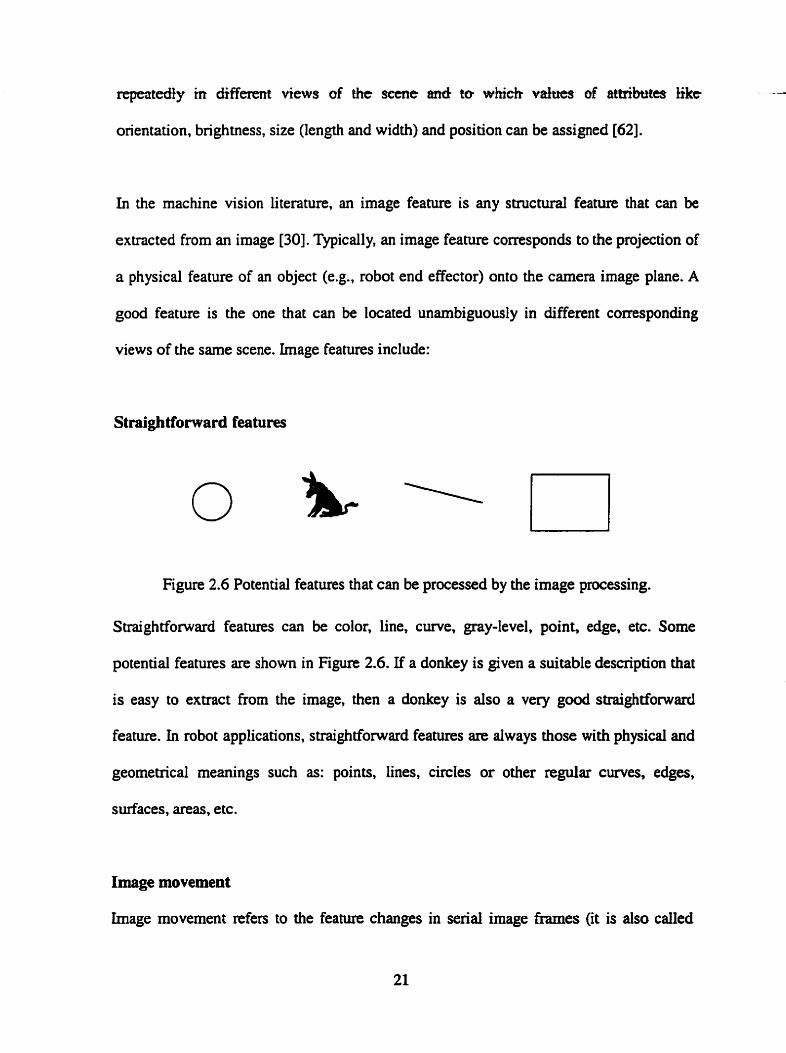
Straightfomard features

Figure 2.6 Potential features that can be processed by the image processing.

Snaightfonvard features cm be color, line, curve, gay-level, point, edge, etc. Some

potential features are shown in Figure 2.6. If a donkey is given a suitable description that

is easy to extract fiom the image, then a donkey is aiso a very good straightforwad

feature. In robot applications, svaightforward features are always those with physical and

geometrical rneanings such as: points, lines, circles or other regular cuves, edges,

surfaces, areas, etc.

Image movement

Image movement refers to the feature changes in serial image fiames (it is dso called

v i h sueam) or finît ordei- or h i g k o~der &riuatiues of the same image These dynamic

features reflect the object movement, as well as camera movement. Jarvis [46] introduced

two distinct approaches for the computation of motion h m image sequences:

Feature-based approaches require that comspondence be established between a

sparse set of features extracted from one image with those extracted from the next image

in the sequence. The effort of finding f e a m correspondence is often damaged by

occlusion, which may cause features to be hidden or false feanires to be addressed' .

interpretation of motion and structure h m optic flow2 requires the evaluation of

fmt and second partial denvatives of image brightness values and also of the optic flow.

The evaluation of derivatives might drarnatically change the content in an image because

it is a noise enhancing operation.

A bstract features

In some special applications, some abstract features based on mathematics without stmng

physical meaning can be used. These features are the resdts of some mathematical

' In practid cornputer vision. motion analysis requires the storage and manipulation of image sequaas cathe~ than single images. Image sequences can be stored in memory as Ws of -YS, vcctors of mys oc 3D m y s , and on disc as single file or as files with scquentiai numbcring, Each image in a sequenct is ofien called a frame, and the elapsed time for forming each fiame is calleci the frame interval. The inverse of the fhme interval (the number of fiames per second) is the hme rate.

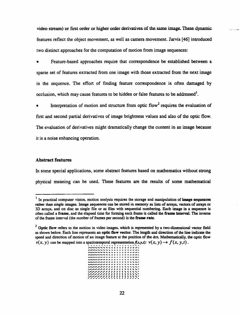
* Optic flow refers to the motion in v ida images. which is representcd by a twoaMcnsiond vcctor field as show below. Each line represents an optic flow vector. The Iength and direction of the line indicate the speed and direction of motion of an image feahue at the position of the dot, Mathematicaiiy, the optic flow

tr;uisformatio11~ (e-g., wavelet transfannatim and Fast Fourier Transfomation ml).

FIusser and Suk [26] classified the features into four types:

Visual features (such as edges, textures and contours)

Transform coefficient featrires (such as Fourier description)

Algebraic features (such as those based on matrix decomposition of an image [37])

Statistical features (such as moment invariants)

The last three types of features are mainly based on the mathematical transformations and

can be categorized into abstract features. The detailed explanation of these feahires can

be found in [26].

Jang and Bien [44] provided a mathematical definition of a feahue as an image function.

They considered an image received by a camera to be a 2D array of iight intemiries. Then

the brighmess intensity of the image at the location (u, v) is 1 (u, v), where

- u, 5 u 5 u,; - v, 5 v 5 v, . (u,, v,) is the origin of the image plane. Then a feature cm

mapping of the locations and brightness intensities of the pixels in the image. The

mapping can be either linear or nonlinear, depending on the nature of the feature under

consideration, and may include Dirac delta functions'.

' Dirac delta fundion 6(1) is not a mie hmction since it cannot k defincd completeiy by giving the

function value for aU values of the argument t. The notation G(t -to) stands for G(t - t g ) = O fw

The selection of features is essential for a swcessfid uision application, G d features are

easy to detect in different noisy backgrounds and could provide effective information to

the application system. Image recognition criteria include feature robustness,

completeness, and cost of feature extraction.

2.4.2 Feature Extractor

Feature extractor is a set of software to explicate some useful features by processing the

image data. Any particular features make certain information explicit at the expense of

some information that is pushed into the background and may be hard to recover [62].

The characteristics of features dictate that the feature extractor must be application

orientated. A typical feature extractor shouid achieve the following three tasks:

Initial processing procedure

This procedure is used to highüght the useful f e a m s in the image. Normaiiy the initial

procedure includes: digitization, thresholding, segmentation, histogram, shape

identification, template match, edge detection, etc. Information on these basic methods

c m be found in any textbooks on image processing, e.g., [74] [89].

Quantization of the feahire parameters

Image feature parameter is any real-valued quantity that can be calculated from one or

more image features [25]. Implementation of robot vision is closely associated with

cornputer calculations, and cornputers cannot work without quantization of feature

parameters. In robot vision applications, common feature parameters include coordinates

and distances between points in image, lm@ d imes or edge4, &r geomeeieel

parameten of lines or curves, etc. Some mathematical transfomations c m be very useful

to obtain distinctive parameters. These mathematical methods include wavelet

transformation. Hough transformation [56], FFI'. etc.

Matching correspondent features

In robot vision applications, obtaining several related images from the stereo or senal

images using the same camera at different times. is very cornmon. Therefore, one of the

important issues is how to tind the corresponding features from the comsponding

images.

This is the most difficult part of feature extraction. Except for sorne special applications

in which extra information about the target (or camera) movement can be obtained h m

other sources, two or more images of the same scenery are needed to recover the target.

The purpose of matching the corresponding features is to find the same features reflected

in different images. Those images are taken from the same scenery but from different

uiewpoint or in different tùne. There are two kinds of methods tu deal with feature

matching problem.

Area-based method: it is a typical method to compute the comlation between two

images in two regions. Fit-order or second-order differential images are used to find the

correlation between two regions. The problem is that sometimes the corresponding points

c m o t be found even if the simiiar areas are found.

F e s t u ~ W methd: Feature-based method is used ta find tbe. same f e â û ~ ~ ~

according to the sarne feanire descriptions such as the same color, or shape, etc. The

features include two categones [33]:

Global fatures such as long edge segments. These features are difficult to detect

in both images. If suitable global features can be found, it will be easy to implement

image matching.

Local fwtures such as edges extracted with local operators. These features are

easy to detect, but it is not easy to be used to match many similar features due to the

effect of noise.

There is no general feature matching method as the technique depends on the

applications. Before choosing a feanire matching method, the analysis of feahires is

required. Appropriate feature analysis could alleviate the workload of feahire matching.

2.5 Reconstruction, lnterpretation and Decision

Interpretation, which refea to the description of the observed object, answers the

question "what is present in the world and where it is". Interpretation is reaüzed by

reconstruction that is an inverse procedure of mapping h m the object to the image.

Norrnally the complete description of the object cannot be realized Sometimes the direct

results from reconsmiction can produce ambiguities. Therefore, a decision mode1 is

needed to process the initial interpretation of the objects.

The goal of robot vision is to obtain information from image sequences rapidly and

reliably to guide the robot to complete its assigned task. As shown in Figure 2.7,

reconstruction can be thought of as an inverse procedure of mapping h m object to

image. Due to the nonlinear and complicated nature of the vision model, the inverse

procedure may generate no solution or redundant solutions. Many researchers have

investigated ways to avoid ambiguities in reconstruction.

projection

target image

reconstruction

Figure 2.7 Reconsmc tion is the inverse mapping of projection.

According to the features used for reconstruction, Maybank [64] discussed two typical

ways to obtain the space information from an image.

Reconstmction fmm static image correspondences

There are many different static features (point, line, c w e , gra wel, color, etc), which

have been used by many researchers to setup image comspondences. In some works.

some vimial and abstract features have been used to recover some special characteristics

of the objects. As the result of this kind of reconstruction, static information of the

observed objects cm be achieved

Refoastmtüon €mm dynamic image corp~sponden~

Image motions have been used in recent decades to deduce the veiocity of the carnera and

the position of one point relative to the camera frame. Analysis of a time-varying image

often involves estimating 2D motion in the image plane. Image motion estimation is very

important in many applications such as object tracking [84].

Huang and Netravali [43] discussed typicd situations of reconstruction from feature

correspondences and categorized them into three types:

3D-3D correspondences: in this case, the locations of N corresponding f e a t m

at two different times are aven, and the 3D motion of the rigid object is estimated

2D-3D correspondences: in this case, some of N comsponding features are

specified in t h e dimensions and the other features are defined by their projections on

the 2D image plane, and the location and orientation of the camera are found.

2D-2D correspondences: in this case, al1 the N corresponding features are given

in the 2D image plane either at two different times for a single canera or at the same

instant of time but for two different cameras. In the former case, the 3D motion and

structure of the rigid object is identifie& and in the lattex case, the relative amh& of the

two cameras is detennined.

Image motions contain information about the motion of the camera and the shapes of the

objects in the field of view. The= are two main types of image motions [64]:

Finite displacement is reconstructed by a finite number of discrete point

correspondences between the two images of one scene iaken at different positions.

* Image v e l e e i k are the veki t ies of rhe points in the image as they mavc over

the projection surface.

In recent years, considerable effort has been devoted to the reconstruction from image

movement. Some of the typical methods are introduced in the following paragraphs.

Spetsakis and Aloimonos [go] introduced reconstruction fmm moving liaes. The

accuracy of the motion estimation results depends critically on the accuracy with which

the location of the image feanires can be extracted and measured. Generally, line feanins

are easier to exmct in a noisy image than point features (e.g., using Hough

transformation). Furthemore, it is easier to determine the position and orientation of a

line to subpixel accuracy than the coordinates of a point.

Faugeras [19] introduced reconstniction from moving curves. Because of the similar

reasons descnbed above moving curves are very wful features in 2D image motion.

Usually more feature parameters are needed to describe the moving curves compared to

the moving lines.

Negahdaripour and Horn [69] introduced reconstruction €rom gray leve1 change. It is

difficult to find suitable features or corners on the image of smwth objects. Furthermore

the feature-matching problrm has to be solved. In this case, the change of gray-level is a

good feature to reaiize the reconstruction.

Wu and Wohn [IO51 inûoduced reconstruction fmm image vdodty estimation. Thc

velocities of points in an image depend an the xmticm af the camera relative ta the

environment and also on the distance from the image plane to the object points.

Theoretically and practicdly image velocities provide a method of reconstruction, which

is an approximation to the more complicated reconstruction. In practical applications, the

estimation of the velocities and positions of objects relative to the camera is often

generated in a short period of tirne.

2.5.2 l nterpretation and Decision

Interpretation is the comprehensive result of reconstruction. In the previous section, it

was mentioned that simple mathematical reconstruction could produce meaningless

results. Sometimes more than one ~constmction procedure is applied in the robot vision

application. The decision procedure can analyze and synthesize al1 the information to

produce meaningf' information about the observed object

In robot vision applications interp~tation can be divided into two categories:

a 3D space interpretation reconstructs the 3D space information h m the

extracted features. Typically 2D image space coordinates and camera models are used to

realize the inverse transformation h m 2D space to 3D space. The geometricd

characteristics of the observed object are dso the main content of description.

a 2D image interpretation is not the simple repeat of the image features but a kind

of synthetic result that c m describe the behavior of the objects in 2D projective space.

Image Jacobian matrix in image space, or the resdts of some puxe mathematical

transformation (wavelet transformation, FFI', etc) can be used to interpret the image.

Decision procedure is ta appiy the infcumîiion obtained finm a vision system to some

practical operations. In robot applications, deàsion output cm be applied to the control

system or for task planning of the system. Though description procedure makes the

reconstruction results very meaningful, complete information recovery of objects is

impossible. Decision procedure decides which part of the information is usehil and

compares it with the information fmm other sensors or other sources. Decision is a very

important step in robot vision application. Because there is no general vision mode1 as

perfect as human vision system. how to apply the results of interpretation in a dynamic

environrnent, as the purpose of a decision procedure, becornes the key point of the

success of a robot vision system.

2.6 Robot Vision Application

Vision sensors have k e n applied extensively in robotic research Iabs, as well as in

indusirial environments. A11 the applications cm be divided into two categones

depending on the purpose of the vision system. Some details about visual servo control

system will be introduced in this section.

2.6.1 Two Types of Robot Vision Applications

It was mentioned in the previous sections that a vision system could answer two

questions: what it is and where it is. A practical robot vision system shodd answer both

of these questions, but often focuses on one of them.

Qurtlity ef Obsewed Objeets (w ha$ ir is)

A typical application for this category is to guide the mobile robot to avoid the obstacles

in its path. Basically the locations of the obstacles should be known, however, the prezise

measurement is not necessary. Recognition of the obstacles should be more helpful for

deciding which kind of obstacles exist in the scenery and then making decisions to allow

the robot to stop or avoid the obstacles by following a specified tmjectory.

Measurement Precision (where it is)

This kind of vision system concentrates on the geometry measurement of objects in the

world. The precision is very important in this situation. Since it will guide the robot

movement, this measurement cares more about some partial geometrical features (such as

points, lines and planes) and ignores the complete quality of the object. A typical

application is visual servo control system that will be discussed in the following section.

2.6.2 Visual S e ~ o Control System

Visual-servoing is a technology that incorporates the vision information directly into the

task control loop of a robot. This kind of control system is not a simple feedback system

but the fusion of results h m many elemental a ~ a s including high-speed image

processing, kinematics, contml theory and rd-time computing 1251. Combined with

sensor fusion technology, a lot of creative visual control techniques have been developed

which encompass manufacturing applications, teleoperation, missile tracking, nuit

picking as weli as robotic table tennis playing 151, jupgiing, etc.

Sanderson and Weiss [76] described the characteristics of different visual semo systems,

which forrn the basis to identify different visual servo applications. According to the

description method of control e m r function, there are two kinds of visual smro

approac hes:

Position-Based Method

In this method, control error function is computed in the 3D space based on an ideal

geometric mode1 of the object. This method requires a calibrated camera to obtain

unbiased results (Position-based look-and-move (PBLM) model as show in Figure 2.8

and Position-based visual servo (PBVS) model as shown in Figure 2.10). The main

advantage of position-based control is that task description in tems of the Cartesian pose

is very cornmon in robotics. The main disadvantage is that this method is sensitive to the

carnera calibration error, and the computation time is longer than image-based method.

Image-Based Method

In this method, control emor function is computed in the 2D space based on the image

Jacobin matrix that shows the characteristics of movement in image space (Image-based

look-and-move @LM) model as shown in Figure 2.9 and Image-based visual servo

(IBVS) mode1 as shown in Figure 2.11 ). Some algorithms provide the camera velocity in

each iteration for minimizing the observed emr in the image. This method is mbust with

respect to the camera and robot calibration e m r s and cornputation time is less than that

in the position-based method. The disadvantage of this method is the presence of posSbIe

Cartesian Robot hntroi Law

-+ Controller

-) Robot -

I I

joint sensors E z l

Figure 2.8 Position-oased look-and-move (PBLM) model.

Figure 2.9 Image-based look-and-move @LM) model.

Based on how to use the visuai information in the robot control system (decision

meihod), two kinâs of visual servo contml systems are defined:

P I jl

- Robot Image space controi iaw

- Robot Controiler

-+

* Dymmit look-and-wve systetn: the h e v d informit€ition is used as the set-point

input for the robot joint-level controller (as shown in Figure 2.8 and Figure 2.9).

Direct visual servo system: the visual servo controller dircctly outputs the

control cornmand to the joint actuator (as shown in Figure 2.10 and Figure 2.1 1).

Considering the description methods and decision methods categorized above, a

comparasion of the four categories is given in Table 2.2.

Table 2.2 Cornparison of different visual control methods

1 ControlType 1 Coordinate System 1 Components of Controller I

The choice of the methods of visual servo control depends on many factors, including the

task description. If a task (e.g., a trajectory tracking) could be described in 2D projective

space without ambiguities, then an image-based system shouid be preferred. Integrating

the vision system into the controller can therefore potentially eliminate the need for joint

sensors, as the location of the end effectm is no longer detennined by applying the

forward kinematic transformation to the joint sensor-derived displacements [106].

PBLM (Fig 2. 8)

IBLM (Fig 2.9)

PBVS (Fig 2.10)

IBVS (Fig 2.1 1)

In industrial applications, look-and-move control system is used more often in robot

controllers compared to visual servo system. The Mons are 1251:

Lower sampling rate of vision system is difncult to provide direct control of the robot

end-effector with cornplex, non-linear dynamics chanicterîstics. Using interna1 feedback

3D

3D

3D

2D

visual controller +joint controller

visual controller +joint controller

visuai controller onIy

visuai controller oniy

can inierndly srabilize the herob.

Simpler construction of robot control system is achieved by look-and-rnove control

system because many robots aIready have an interface for accepting velocity or

incremental position commands.

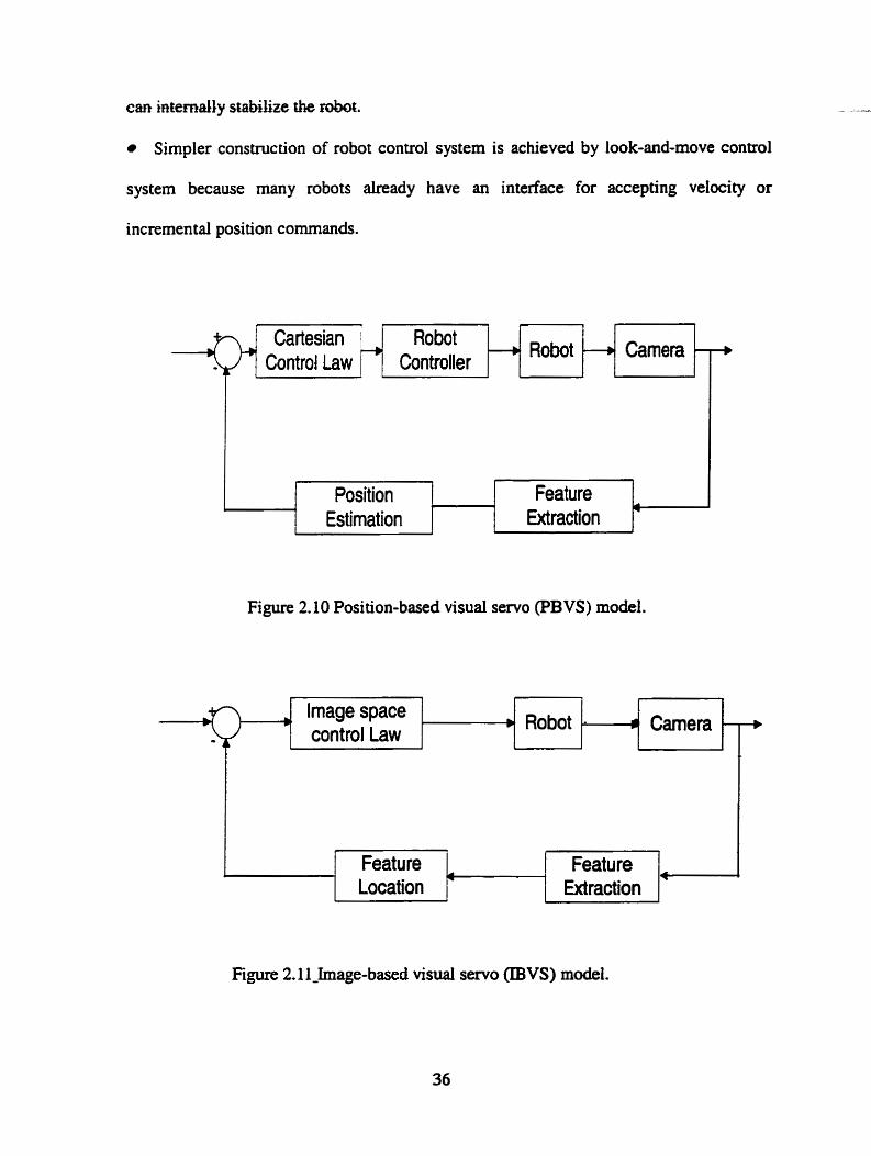
Figure 2.10 Position-based visual servo (PBVS) model.

ri Camem

J

+

4

Featu re Extraction

Position Estimation

Figure 2.1 1-Image-based visual servo (IBVS) model.

'

Robot Controiier

Cartesian control Law

4

Carnera b

.

1

+

r

Robot ' Image space controi Law

Feature Featu re Location Extraction

Successful robot vision systems are al1 based on the flexible integration of hardware

(such as camera placement, marked object, and illumination) and software (such as

feature selection. task description, and image processing). Some of the typical application

exainples will be discussed in this section.

In 1973 Shirai and houe [84] designed a vision system for a robot to grasp a square

prism and place it in a box. This was one of the earliest visual feedback applications. A

camera was fixed and edge extraction and Iine fitting were used to determine the position

and orientation of the box.

In 1988, Kabuka et al. [47] used Fourier transformation to center a target in the image

plane. An IBM-PCIXT cornputer performed the computation, and the targeting

pmessing took about 30 seconds.

Tracking and grasping a moving target is an important application for robot vision.

Andersson f51 intmduced a d-thne vision-assisted robot ping-pong player. He

developed a 60 Hz, low-latency vision system. Special chips were designed to calculate

the centroid of the ping-pong bal1 accurately in the image plane. The aemdynamics of the

bal1 was used to generate accurate predictions of the position of the ball. Zhang et al.

[107] intmduced a visual servo system for a robot with eye-in-hand placement, which

could pick up items h m a fast moving conveyer. Prediction algorithm was applied to

increase the response of the vision system. M e n et al. [3] used eye-to-hand stereo vision

system to mck a fast mwing t;ngn (2fOmmls). Hoastnmgi f381 presented e viskm

system with a fixed overhead camera for a PUMA 600 to p p a moving target.

Skofteland and Hirzinger [86] discussed capturing of a free-flying polyhedron in space

with a vision-guided robot. Lin et al. [57] introduced an approach for catching moving

targets. The fint step was couse positioning of the robot to approach the target; the

second step was "fine-tuning" to match the robot acceleration and velocity with the

targe t.

Vision system could be more efficient when combined with other sensors. Feddema et al.

[24] and Feddema and Mitchell [25] presented a feature-based trajectory genenitor, which

provided smooth motion between the actual and desired image features. Image features

could be taught off-line either through teach-by-showing techniques or through CAD

simulation. A PUMA robot was used to track a gasket on a circular parts feeder. The robot

was not allowed to travel near a singularity configuration. The authors pointed out that an

important characteristics of the feature-based trajectory generator was that features

provided by joint sensors with different sampling times could also be used, thus ailowing

a unified integration of sensors

Harrell et al. [32] used visual servoing to control a two DOF fruit-picking robot as the

robot reached the fruit. Ultrasonic sensors were used to detennine the distance between

the Fniit and the gripper.

Rives et al. [73] and Castano and Hutchinson [Il] used task function method to position a

target with four circles as the feaairrs Hashimatn et aL €34 apphed position-based and

image-based visual servo systems to a PUMA 560, which tracked a target moving on a

circle at 30mm/s. The results of two visuai-servo rneâhods were compared.

Castano and Hutchinson [ I l ] introduced a visual cornpliance method with the task-level

specification of manipulator goals. The motion estimation was a kind of hybrid

visiodposition measurement structure. The two degrees of freedom, which were paralle1

to the coordinate axes of the image plane of a camera, were decided by image-based

visual measurement, the remaining degree of freedom, which was perpendicular to the

camera image plane, was obtained by the robot joint encoder. The first two rows of the

Jacobian matrix dated to differential changes in the robot's motion to the differential

changes in the image observed by a camera. The third row of the Jacobian ma& related

to differential changes of the robot's motion to differential changes of the perpendicular

distance between the robot end effector and the camera image plane. A PUMA 560 robot

was used to perform various tasks. In order to alleviate the difference in time delay for

the vision processing and joint sensor processing, an LED was attached to the robot end

effector to increase the speed to recognizing the target.

Tendick et al. [94] discussed the possible applications of vision system for tele-robots.

The task was considered to be specified dynamicaiIy by human operators according to the

selected features from the image.

Hager [29] applied the projective geometry to the image-based visual control systern with

eye-ta-hand came= arrangement. Projective geo- was used for &e calibrahm of

robot and camera parameters and for defining the setpoints for visual control that were

independent of the viewing location. The author introduced the mathematical description

and related Jacobin maaix for three typical robot tasks: point-to-point, point-to-line (a

motion that a point moves to any points on a line) and line-to-line (a motion that a line

moves to be digned with another line). As an implemented exarnple, a Zebra Zero robot

a m was used to insert a floppy disk into the floppy disk driver of a compter.

Jang et al. [45] presented the concept of Augmented Image Space (AIS) and Transformed

Feature Space (TFS). AIS is a sensor based space generated from the acquired image and

the depth information extracted through some motion stereo' algorithm. Based on AIS,

TFS is constructed with a finite number of defined features. In the expriment, eye-in-

hand system was used and the desired features in AIS were obtained through "teach by

showing" method. This method avoids an exorbitant amount of on-line computation to

determine the position of objects from their images. The huge amount of computation

could degrade the stability of the system.

Al1 of the above mentioned works are "passive vision" applications. As the application of

active vision, Agin [2] proposed to use hand-held light stripes in order to simplify image

processing procedure. The specified light stripes supplied extra information for image

processing procedure. Venkatesan and Archibald 1971 described a system with two hand-

A major difficuity in the anaiysis of p i c m of a 3D scene is the lack of dWct depth infortnation in a single picture. A progression of views of a scene is available if the observer is moving with respect to the environment, hence the use of the tenn ''motion stereo" [70] [ 1031.

held laser scamiers fur d - t h n e mtd of a 3 EKE robot.

Another control method with active vision is mobile camera head that was introduced by

Gilbert et al. [27]. The purpose of this control was to adjust the pose of the carnera in

order to track the movement of a target. The control system tried to keep the m e t

always at a fixed place in image plane.

2.7 Fault Tolerant Robotic System

In 1942, Asimov [6] adciressed the robot safety issue with his famous "kee laws of

robotics". Nowadays robots are being more fkquently utilized in inaccessible or

hazardous environments [66]. Fault tolerance is highly desirable in these environments

because the results of system failures may be very dangerous and unrecoverable.

Researchers have considered the use of redundancy and safety checks at the joint and

actuator Ievels, and aiso in the software and control architecture [31]. Dhillon 1161

analyzed various factors that influence the robot reliability and safety.

Visinsky et al. [99] divided a robot fault tolerant system into t h e layen: a continuous

servo layer, an interface monitor layer, and a discrete supemisor layer. Servo iayer fadt

tolerance requires the controller to control the robot movement when some failure

happens. Interface layer contains the trajectory planner and provides fault detection and

some basic tolerance functions for the system. S u p e ~ s o r Iayer provides a higher-ievel

fault tolerance and general action cornmands for the robot.

Waiker and &tvdle~o [1@1] us& fad l bees €0 &yze robot fai~u~e6 & d y on the -

sensing failun. Redundant kinematic and actuators design is also an extensively

addressed topic [66]. Huang and Notash investigated the failure modes, causes and

effects of a parallel manipulator [40] and studied the failure situation of a parallel robot

DEXTER (made by MD Robotics Ltd.) by using the failure mode and effect analysis

(FMEA) and fault tree analysis (FTA) [41].

2.8 Summary

Generally, the whole application procedure of robot vision can be treated as a series of

space u?uisformations, which cm be divided into three steps:

Step 1. Transformation from 3D world space to 2D image space by projective mode1

Step 2. Transformation from 2D image space to feature space by image pmcessing

Step 3. Tmsformation from image feature space to 2D space or 3D world space by

reconstmc tion mode1.

The dated technologies of vision application include projection geometry, image

processing technologies, control technologies and suitable decision making methods.

It should be noted that despite the long history of using vision to guide robots, the

applications of this technology remain limite& The robot vision models are far fhm

perfect cornpared with human vision. However many projection models and image

processing methods based on the mathematical development have been successNly used

to simulate the performances of the cameras and obtain useful information from the

images taken from the observed objects.

There are two types of robot vision appicatians based on the purpose of the vision

system. Vision system can be used to find "what it is" in the scenery, as well as "where it

is". Based on the observation of "where it is", visual servo control technology has been

developed in the research labs.

Robot vision technology provides a combination of flexibility, adaptability, precision,

noncontact rneasurement and object recognition for robotics. This technology is

involved with diverse technologies. the development of theories and equipment, this

technology will have a bright future.

Vision-Assisted Robot Kinematic Error Estimation

3.1 Introduction

Robot kinematic error estimation is the cornparison between the required motion

description and the actuai motion description. Robot kinematic error could be produceci

by a sensor or by a part of the mechanism. such as faulty calibration errors or

transmission backlash, respectively. Vision-assisted robot kinematic e m r estimation

realizes the kinematic error estimation using the information obtained from the vision

system. The usual robot motion description is a bbtrajectory" used to describe the sequence

of positions, or velocities that the user of the robot has specified in different reference

frarnes. Task description c m be very different in differemt reference frames, and hence

influences the integration of the vision system and the measurement resuits of the vision

system. Based on the methods of the task description, d i f fe~nt kinematic error estimation

methods will be intmduced in this chapter.

The vision system c m transfomi the observation of the robot motion into the image form

Therefore, robot motion description c m also be defined in the image space, and a series

of methods have been developed to retneve the information of 3D space h m 2D image

space (refer to Section 7-5). These methods simulate the image formation procedure and

the transformation among the different spaces.

According to the robot taslc quiremen& ÿisio~~asktedrnbot îchmtic. ermr e s h a t h

can be completed in robot space, camera space or image space. Usually the estimation

results are represented in or tmsforrned into 3D robot space or camera space. However

in some cases, the transformation is not necessary if the required task motion and the

acnial motion cm be both described in the image space. In order to simpli@ the

kinematic error estimation and lead to a successN vision application, the correct

selection of the reference frame to describe the robot task is quite important. SpeciaI

robot structure can also simplify the procedure of the vision system to obtain kinematic

infornation of the robot.

Vision-assisted kinematic error estimation cm be applied to any applications that need

the motion information of the robot. There an two kinds of basic applications:

Vision is directly incorporated into the task planning and contml of robots, such

as a visual servo control system. A case study will be introduced in Chapters 4 and 5.

Vision is used for the evaluation of the robot performance, such as supervishg the

robot motion to make some decisions related to safcty or integrating the related

machinery harmoniously with the robots. A typicai application is to improve the fadt

tolerance of a robot that will be discussed in Chapter 6.

3.2 Motion Description in Different Reference Frames

One of the ultimate goals of robot vision is to mate autonomous robots that will accept a

high-level description of tasks and wiU execute the motion without human intervention.

Therefore, a proper description of the task in a suitable mathematicd fonn is an

important issue for mbot vision appheatioii. Fm differen~ motion desenptions, differenk

parameters are required to decide the mathematical fom. An observer, such as a vision

system, can obtain those corresponding parameten.

As shown in Figure 3.1, a robot task could be represented in different reference fiames.

These reference frames are usually but not necessarily are in the form of coordinate

frames. The vision system could not only perform direct observation of the image

features, but also perform the role of the recognition observer and joint observer (as

shown in Figure 3.1) through suitable mode1 transformation. Image formation procedure

c m be considered as the result of three lcwls of space transformations, which will be

discussed in the following sections.

I Task Definition

Recognition m I 4 t - Robot Joint

Frame Observer -

Figure 3.1 Task description and observation with vision system.

The observer couid consist of various. which could ped(i17n the 0 b a a t i ~ task

and provide the robot system with the necessary information to carry out the desired

tasks. A vision measuring system provides more choices for robot motion description.

However, sometimes in a complex vision system, traditional joint sensors are still needed

to observe some specific variables of robot motion.

3.2.1 Transformation from Task Space to Robot Space

The task definition for a robot cm be the symbolic representations of the objects and

relations between the robot and the objects, as well as attributes describing the robot

configuration in the world coordinate frarne. The task description could be in the fom of

a simple sentence such as "let the end effector grip a part on the conveyef'. It could aiso

be in the fom of the complicated logic representations, or even some gmphics.

A general robot system cannot ded with diverse representations of the tasks. A typicd

task representation is a tmjectory described in robot coordinate h e s , such as the

motion of specific points on the robots, which are represented in the robot base

coordinate frame. Base and end effector fiames are used very of'ien in robot vision

applications, because most of the time a robot vision system should supervise the motion

of the end effector andior some objects located in the world space. Usually the world

space will be assumed to be the same as the base frame, and then the motion of the end

effector and the objects in the environment can be described in the same robot base

frame.

3.2.2 Transformation from Robot Space to Camera Space

The camera is a necessary cornponent of a vision system. One of the important tasks of

the vision system is to find the relative positions between the objects in the environment'

with respect to the camera. Therefore, if the task could be defined in the camera space, it

would simplify the transformation procedure.

Generally, the position information in the camera frame is required to be msformed into

the robot space. Then the position of the camera with respect to the world f m e should

be detemiined pnor to identibng positions of objects in the camera frame. This

procedure is called carnera calibration. Cmera calibration is the process of determining

and relating the 3D position and orientation of the camera with respect to a certain world

coordinate frame. Carnera calibration is dso referred to the mapping between the 3D

coordinates and the 2D image coordinates.

Three methods for camera placement were introduced in Chapter 2, where each method

has a different effect on the results measured by vision. The camera calibration procedure

for an eye-in-hand system is to detennine the camera position in the moveabie end

effector frarne. Where as the camera caiibration procedure for an eye-to-hand system is to

determine the camera position in the fixed robot base bme (world fiame).

' Environment refers to al1 the space arotmd the robot. The obsmable space for the camera Q -eV. When the camera rnoves, the scenery is variai. The scewry is also influenceci by the change of the physical parameters of camera, such as focal leagh, fieid depth, etc. T ' h a art many objecCs in the environment or sceneq, but ody some of them are necessary to be processed by the vision system, which are calleci targeted objects or simply targek. If ody som specid points on the targeted object art processed by the vision system, those points are caiied targeted pohîs or f'îure points.

For an eye-to-hmct system, the festxlts of the transfonnation of the points m e fu&

object in the environment are more precise than those of the transformation of the points

on the robot, because the relative position between the world frarne and the camera m e

are fixed, but the relative positions between robot joints and the camera are varied.

On the contrary, for an eye-in-hand system, the results of the transformation of the points

on the robot are more precise than those of the points on an object in the environment.

This is because the relative position between the camera and its attachment point on the

robot is fixed, while the relative positions between the objects in the environment and the

camera frame are varied. If the targeted objects in the environment move as weU, then the

result of transformation from the objects in environment to the carnera space could

produce additional errors due to the errors in the camera calibration.

For the active camera head, the situation is similar to the eye-to-hand system, but an

additional problern is that the calibration should be performed dynamically because the

reference point of the camera frame is varied as the camera head moves. Even if some

fixed reference points are assigneci in the scenery, it is sti1.l uery difncult to get d - t i m e

precise measurement results of the points on the robots and the objects in the

environment due to the motion e m r of camera,

3.23 Transformation from Camera Space to Image Space

In a vision system, images are the major sources of information that could describe the

motion of the robot and the objects in the environment. nie transformation h m cameni

space tcr image space is an essentid psocedue. This transfonnatiios is also called --

projective model or camera model. This transformation has been referred to as the

correspondent between 3D features and 2D features by some authors [43]. The image

coordinate frame is set up on the image plane of the camem. Because-an image is formed

by displaying a matrix of pixels in the proper order, the coordinates in image fnime are

digital coordinates.

Several carnera models will be introduced in the following sections. There is no camera

model with absolute precision, and the inverse transfomation to obtain the positional

information in 3D space is often non-linear with multiple solutions.

3.3 Projection Models and Reconstruction

The projection model can develop the corresponding image of the observed object if the

the-dimensional position of the observed object is given. The reconstruction mode1 can

determine the three-dimensional position of the observed object if an image of the

observed object and the relative positions of ail the comsponding image fanires are

given. If error estimation in 3D space is needed, a reconstruction procedure is an essential

process. Reconstruction is the process of detexmining and relating the 3D positions and

orientations of the observed objects from their image spaces. TheoreticaUy,

reconstruction is the inverse process of projection (refer to Figure 2.8). The

reconstruction model can be developed h m the corresponding projection model. The

problem is that the mathematical reconstruction results are nomally not unique, and

more conditions should be searched in order to obtain practical reconstruction results.

Three commonly used projection models are: cenaal perspective pmjection madel, scded . . . . -. . . .-

orthographie projection mode1 and affine projection modei. They are d i simplified from a

general projection model, which cm be represented in homogenous coordinates as [5 11:

where ' p is the 3 x 1 position vector defined in 2D image space, " p is the 4 x 1 position

vector defined in the 3D task space, T is the 3 x 4 transformation matrix projecting the

3D reference frame ont0 the image m e .

view point

, Y . image plane 1 --

Figure 3.2 Transformation h m camera h e to image fiame.

Figure 3.2 shows a coordinate frame denoted by X, Y, 2, for a single camera system. The

observed object is a point in 3D camera space: 'p = Lx, y, z]', and its coordinates are

expressed with respect to the camera coordinate frime, Fc. The point 'p is projeaed onto

the image plane Fi with coordinates 'p = [u, vlT. d is the perpendicular distance between

the observed point and the viewpoint, f is the focal length. The three different projection

models wiU be discussed in the following sections.

3.3.1 Central Perspective Projection

Central perspective projection is the most common model in vision research. This model

is suitable when the center of projection (focal center) is at the origin of the camera frame

and the axes of a camera coordinate frame are aligned with the axes of the world frame.

With necessary error compensation, this model could produce accurate measurement

results.

When the projective geometry of the carnera is modeled by cenaal perspective

projection, the carnera model is represented as:

This transformation correctly models a perfect pin-hole imaging process. Unfortunately,

the resulting solution is not linear due to the dependency on the distance 2, which is the

denominator in equation (3.2). The reconstruction is not unique because the 3D

coordinates [x, y, z]* are decided by two formula in equation (3.2). Physically, a point in

an image cm be the projection result of aoy point on the same ray in 3D space. In order

to recover the depth information, z coordinate, multiple views or knowledge of the

geometric dationships between severai feature points on the target are needed. In

practical applications, this mode1 is sensitive to the subtle changes of camera positions

and to the background noise [95].

In order to calculate the depth (z coordinate of a point on target), it is assurnecl that two

fixect cameras are used and two pictiaes fimm Che same stew rue taken. Tks obsewed

point is O p = [x, y, zjT in the robot base coordinate hune. The transfomation rnatrix h m

the left and right image coordinate frames to the base coordinate f m e are TLo and Tc, ,

respectively. It should be noted that Tl,, and T,, are imown initially from camera

caiibration. Then the coordinates of 'p in the left and right carnera frames are

'P, =[xi Y, z J =T,,(Op)

'P, = Lxr Y, zrr = TrJOp)

The left image of the point 'p is 'pi = Cui, vil ' and its right image is 'p = [ u , WJ '. The

focal Iengths of the left and right cameras ~IX assumed to be equal: fi = f, = f. Using

equation (3.2), equations (3.3) and (3.4) can be cxpressed as:

Equation (3.6) is a function of the coordinates of point Op defined in the robot base fnime.

There are three unknown variables, which are the coordinates of Op, and four equations

(according to the matrices in equations (3.5) and (3.6)), so it is possible to reconstruct the

3D space information. The other aspect of this problem is the calcdation of the rna&ices

TLo and Tc,. Because both TL, and Tc, are 3x3 matrices, there are 18 entities to be

calibrated. When the intemal calibration of camera is also considered, there will be more

unlaiown parameters [95].

In or&r to recouer the deph information (the distance b e e n the abject and the image

plane), human eyes use a 5 a t variety of vision-based depth cues, which include texture,

size perspective (change of size with distance), binocular perspective (inward tuming

eyes muscle feedback), motion parallax, and relative upward location in the visual field,

occlusion effects. outline continuity and surface shading variations [46]. In order to

simulate the function of human vision, some active vision techniques have been

developed [46], including using striped iighting and grid coding with special light effects;

identification of relative range from occlusion cues; calculation of depth from texture

gradient; calculation of the range from focusing; calculation of surface orientation from

image brightness; calculation of the range from stcreo disparity; and calculation of the

time-of-flight range.

3.3.2 Scaled Orthographie Projection

If ail the points could be considered in the same plane with the same average distance d

to the image plane, the previous transformation, equation (3.2), could be approximated by

the scaled orthographie projection:

where s is a fixed scale factor, s = aY; and d is the average depth of the centroid of the

observed point set which are located by the cament Obviously the transformation is

changed to be a linear procedure. This transformation is only valid when the relative

depth of the points in the scene is small enough compared to the distance from the camera

to the scene so that the depth can be assumed to be constant. For a large object close to

the h e m , ih is approximation Wones invaüd. Itemlivelysded odopphic

projections can be used to approximate the real perspective for al1 cases [15], if some

local areas of the objects cari be assumed to satisfy the conditions for the scaled

orthographic projection.

The inverse procedure of the scaled orthogonal projection is easily developed:

An image may be locally well approximated by the scaled orthographic projection (also

called weak perspective), but the centrai perspective projection (full perspective) is

required globally to accurately represent the entire scene. The total depth variation across

the scene can be large, but each individual object may satisQ the weak perspective

approximation. Therefore, it is possible to divide the scene into different areps each with

a different depth for its centroid.

It should be noted that when s = 1, then the model is reduced into a standard orthogonal

projection (as shown in Figure 2.3).

33.3 Affme Projection

An affine projection model is simplifieci by letting t31, t32 and t33 e q d to O, in the

transformation maaùr T given in equation (3.1). The affine projection physically does not

correspond to any specific projection situation. The advantage of the affine projection is

55

that it is a good local epproximarion of the peapective p~ojection that accaunts for: both -A

the extemai geometry of the camera, which relates to the position and orientation of the

camera, and the intemal geometq of the lens, which relates to the physical structure of

the camera. The linearity of the mode1 simplifies the camera calibration greatly. Based on

the affine projective geometry, some abstract geometry invariant characteristics

originated from the transformation between images of the same scene, taken fmm

different viewpoints, have been developed [109].

A general affine transformation f: Rn + Rm is a transformation that can be written as

' I I - , where A is an m x n ma& in R"",

called the defonnation matrix of f, and b is a m x 1 vector in R" , cailed the translation

vector of €.

If it is assumed that the projective geometry of the camera is modeled by the affine

projection, then the aansformation h m Che coordinates in the carnend space to the

coordinates in the image space can be show as:

where Te is a 2x3 transformation rnatrix and b is a 2x1 vector.

U s d y more cameras are quired when affine projection m~dels are used for the . .

reconstruction procedure. The invariant geomeaical characteristics [log] between the

projection procedures of different carneras are used to simplify the calibration procedure

and feature matching between the corresponding images (raken from the same scene).

Similar to the analysis in the centrai perspective projection, in the affine projection it is

assumed that two fmed cameras are used and each camera takes one picture h m the

same scene. The left image of the point is = lur, vil and the right image of the point is

= [u, vJ T. Equation (3.9) can be rewritten as:

In equation (3.10) Taml and Tarnmr are f i n e transfomation matrices for left and nght

carneras. Considenng (3.3) and (3.4), (3.10) can be represented by

In equation (3.11) there are three unloiown variables, which are the coordinates of Op, and

four equations, so it is possible to reconstmct the 3D space information. Here only 16

parameten (12 entities for the 4x3 matrix G and 4 entities for the 4x1 vector b) need to

be calibrated 1521.

Actuatly, a pctÏcal canera modtt has mare catibratiorr parameters ttiair the nititiff iir

those transformation matrices men tioned in equation (3.1 1). Depending on the required

accuracy, different calibration methods cm be applied. Tsai's paper is a guod reference

for camera calibration [95].

3-34 Digitization Error

In addition to the error from the projection model, the other important enor source is the

digitization. The anaiog coordinates [u, v]' of a point on an image plane cannot be

accessed directly when using a standard video system (e.g., CCD camera, digitizers, and

frame grabbers). OnIy digital coordinates that represent the horizontal and vertical entries

of a digital image array stored in the computer c m be accessed. However digitization

error during quantization procedure cannot be avoided. If âu and Av represent the

horizontal and vertical sampling intervals. [1, 4T denote the digital coordinates of an

image point ( in ternis of the position of a

coordinate of the center of the image plane, then

pixel), and (Io, &lT denote the digital

the following relations will hold:

Digitization is an important factor that influences the vision measurement result. Au and

Av are decided by the resolution of the image and the optical distortion of the camera

dong different directions.

3.4 Position Error Estimation in 0)Herent Forrns

If the robot task can be descnbed in different spaces or frames, then the robot kinematic

error estimation can aiso be performed in different spaces (3D robot space, 3D camera

space or 2D image space). This will provide different foms for the robot kinematic error

estimation.

Camera placement (as discussed in Chapter 2) is an important factor that can influence

the result of kinematic error estimation. It changes the relationship between camera space

and robot space. In this section only two kinds of camera placements (eye-to-hand vision

system and eye-in-hand vision system), which have been used cornmonly in robot vision

applications, will be considered for the analysis of position error estimation.

The position e m r estimation is the basis of the robot kinematic error estimation. As an

example, a point-to-point positionhg task is considered in this section. The position error

estimation of points on an end effector is the basis of the foliowing kinematic e m r

analysis. This task requires a point on the robot with the end effector cwrdinate ep to be

rnoved-to a fixed or moving point s with the help of a vision system.

3.4.1 Generai Form for Position Error Estimation

According to the camera placement, two models of position e m r estimation cm be

given. In the general fom, the measurernent results from the vision sysrem are used

direcdy without consicking. the pmcedure ficm the camera fiame to the mbot framc and - -

the reconstruction procedure from the image space to the camera space.

1. Eye-to-hand system: In this model, the camera is fixed in the environment and is

calibrated with respect to the robot base frame, as s h o w in Figure 2.4. The position emr

is calcuiated in the robot base frame as [30]:

Ew(T "S. t ~ ) = " ~ - o ~ = T o , e ( ' ~ ) - o ~ (3.13)

where To,e is the transformation matrix from the end effector frame (e) to the base fiame

(O). Op and Os are the coordinates of points p and s in the base coordinate frame.

II. Eye-in-hand system: In this model, the camera is mounted on the robot and is

calibrated with respect to the end effector frame, as s h o w in Figure 2.5. The position

error is cdculated in the robot end effector frame as [30]:

"E,(T,,. Os, ' p ) = ' ~ - ~ s = ~ p - T , , ( ~ s ) (3.14)

where Te,. is the transformation matrix h m the robot base h e (O) to the end effector

frarne (e).

Equations (3.13) and (3.14) demonstrate the general formula for position e m r calculation

in the robot base frame and end effector frame, respectively. The following sections will

intmduce the position emr estimation forms integrated with the measurement procedure

of the vision system.

3-42 Diffemt Cases for Posigion EPPOF EGfj.nBfjOn

The values of T, s and p in different reference frames, as discussed in Section 3.4.1,

might be estimated from the vision measurement, which cm be represented by ?, 8 and

fi, respectively. f , S and fi cm be thought of as estimation of the parameters and can

be obtained from the robot calibration, camera calibration and reconstruction procedure.

The calibration and reconstmction models should be completed before estimating the

kinematic enon. Al1 the estimated parameten can be identified either statically (before

beginning the task) or dpamicaily (duing the execution of the task). Depending on the

application environment, some of the parameter estination procedures are not required.

Case 1: Error estimation calculated in the robot base €rame or end effixtor €rame

In this case the vision system helps locate the position of the target point s in the world

space. The point on the end effector, 'p represented in the end effector fnune, is assumed

to be known accurately and does not need to be rneasured (estimated) by vision system.

For an eye-to-hand system, the vision-measured position of point s should be transfemd

into the robot base coordinate hune before estimating the position error. The procedure

cm be represented as:

* 1 C A

Em(To.etTo,c, s, e p ) = ~ o , e ( e ~ ) - f " J c ~ ) (3.15)

Here, thRe estunation procedures are needed to decide the values of the following

quantities: fo,,, shows robot calibration (hm robot end effector h e to robot base

frame); shows camera cdibration (fiom carnera h e to robot base fiame);

shows reconstruction results from images.

For an eye-in-hand system. the vision-measured position of point s should be transfemd

into the end effector coordinate frarne More estimating the position error. The procedure

can be ~presented as:

'E, ('Î'eî;, , 'S. 'p) ='p - feî;, ('5) (3.16)

Here two estimation procedures are needed to decide the values of the following

quantities. , shows camera calibration (from camera Frame to mbot end effector

frame); 'î shows reconstruction results h m images.

Case 2: Error estimation caIcuIated in the carnera frame

In this case the same camera can see both targeted point s and the point p on the robot, so

the position information of s and p cm be recovered h m the image information. The

error estimation can be computed in the camera space, which is s h o w as:

= ~ ~ ( ~ g , Cp) (3.17)

Because both s and p can be recovered from the same reconstruction model, only the

parameters of the reconsmiction model should be estimated ActuaiIy the point p can be

anywhere on the robot as long as both points p and s can be watched at the same time by

the camera when the robot or camera moves.

L meriy applications, enw esgrnation in the robot spaee is mxkd and eould be

calculated from as discussed below.

For an eye-to-hand system, the transformation from the camera frame to the robot base

frame is needed:

O E, (TOac, '6, 'fi) = ('fi) - ('s) = (cfi-c~) = CS E~~ (3.18)

Here two estimation procedures are needed to decide the values of the following

A

quantities. T,, shows camera calibration (from camera Frame to robot base m e ) ;

and 'fi show reconshuction results from images.

For an eye-in-hand system, the transformation h m the camera frame to the robot end

effector frame is needed:

Ci

C EPP (Tu 's, = ?eT,,(Cp) - *e,(C~) = T,,,(c+C~) =TUC~, (3.19)

Here two estimation procedures are needed to decide the values of the following

A

quantities. Te, shows carnera calibration (hm camera frame to robot end effector

frame); '6 and 'fi show reconstruction results from images.

Equations (3.18) and (3.19) show that the position enor in the robot space codd be

calculated From the position e m r in the camera space by suitable coordinate

transformation. But ihis transformation matrix, which represents camera calibration, is

unknown and needs parameter estimation. The emrs inaoduced h m the carneni

caübration procedure will affect the resuits of the kinematic ermr analysis.

Case 3: &€OF estiniatiorr in the image spaee

In this case both the targeted point s and the point p can be seen by a camera. The images

of these two points c m be taken at the same time or separately at different times. There

are some cornmon features of the two points that cm be detemÿned from their individual

images and the features can be described by mathematical form.

If fd and fa stand for the desired and actual image feanire vectors' of the observed points.

respectively. then the error estimation in image feature space is

i E,(f,,fd) = f a - fd (3.20)

Obviousl y, reconstruction from the images, robot calibration and camera calibration are

not needed any more. fd can be found directiy using the projection model (which is

calculated from carnera model andor geometry model), or using a "teach by show"

approach in which the robot is moved to a goal position and the corresponding image is

used to compute a vector of desired image feature parameters. Robot tasks are thus

specified in the image space, not in the world space. fa is found by an image processing

procedure on the images taken fmm the scenery.

It is obvious that camera model calibration is still necessary when fd is calculated using

the camera model. However, in this situation the 3D position of the desired point with the

' In cornputer graphics, any characmistic description of an image or a region in an image is d e d a feature. An ordemi set of features that may be used to describe artas or objccts within an image is d e d feature vector. A point in the space can be describeci using many diffcrent features in the image s p e The feaîure of the point can be simply the coordinates in image plane; the brightness or der, or even s ~ m c absolute mathematical quantity. Aii the selected description parameters of the point can fom an image fea- vector of this point

feature vector fd is ~ ~ m a l l y a geomeeical poing Iwated in space that kas no relationskip - -

with a physical point. This situation simplifies the calculation of fd and increases the

accmcy off' SO the result of image-based solution is less sensitive to the emrs fimm the

camera mode1 cdibration.

Another important point about image-based error estimation is the fact that except for the

case that the desired and actud points are on the same ray with different depth, when the

image error estimation is zero, the kinematic emor in 3D space must aiso be zero.

Table 3.1 Cornparison of vision-assisted kinernatic error estimation methods.

As rnentioned in Case 2, the error estimation in robot space is needed in many

applications. The relationship between the position enor estimation in robot space and

the position e m r estimation in the image feature space will be discussed in Section 3.5.

I no

no I no

Eye-in-Hand System

g 2 . œ

8 ' Pi: 5 . CiI

3 . C)

2 ,

Eye-to-Hand S y stem

0 U a 3 a 41 u 3 g 5 8 a

Recons~ction

Y=

Y-

Robot calibration

no

no

calibration

Y=

no

Reconstntction

YeS

YeS

Robot caiibration

YeS

no

îamera cdibration

YeS

no

Table 3.1 summines the different e h ~ t e & i c s og emr &madon procedures in the

robot space, camera space and image space for the eye-to-hand and eye-in-hand camera

placements. Ln the table, "yes" ("no") means calibration andor reconstruction from

image features are (not) necessary theoretically.

3.5 Feature Jacobian Matrix

3.5.1 Definition

In order to achieve the transformation from the image feanire space to the 3D space, it is

necessary to develop a relationship between the feature vector and the coordinates in a

3D space (robot space or camera space). The feature Jacobian matrix J can be used to

describe this kind of transformation.

The relationship between the error estimation in the 3D robot space and 2D image space

could be written as follows:

'EPP = J .EPP (3.2 1)

where shows the emr estimation in the 3D robot space or 3D canent qmce.

Equation (3.21) shows the relationship between the m r in 3D robot space (or camera

space) and the image movement.

If 3 point p is rigidly attached to the end effktor with coordinates of [x, y, zlT defined

with respect to the robot base frame, when the robot moves in the 3D workspace, then the

verocity screw of point p in the base f m e is r=B, i; i. q, q, qfl The ftatmc

Jacobian matrix J is defined by

f = ~ , , i

where the kxl vecior f shows the rates of change of the image features (parameters), k is

the dimension of the feature vector f and rn is the dimension of the task space (it might be

robot space or camera space depending on the space in which the task is described). The

k m Jacobian matrix J is calculated as

Jacobian matrix J is determined by the image feanire types and projection model.

Jacobian matrix performs the mathematicai description of the procedure from the robot

space to the image feature space.

If the pose r of the point in the 3D space is required to be caiculated from the f e a m

vector f, then the calculation of the inverse of Jacobian matrix is necessary. In practicai

applications, there are three cases of the Jacobian matrix cdcuIation:

If the dimension of feature vector is equal to the dimension of robot task space,

Le., k = m; and J is non-singular, then the inverse of J exists and is unique and

'E, = J-' 'E, . This means that the number of featwes is equal to the number of

degrees of &dom in the image-based system [24].

If the dimension of featine vector is larger than the dimension of robot task space,

i.e., k > m, then rank of J is required to be equal to rn in order to obtain a solution for

J+ = (J'J)-' JT . In a practical robot vision system, it is very cornmon to use more

features than the degrees of freedom of task space [35] [Ml .

If the dimension of f e a m vector is less than the dimension of robot task space,

i.e., k c m, this means that the number of features is not suffkient to uniquely determine

the motion of the observed object. 'E,, =J' 'E,, + (1 - JiJ)h may be used to obtain

the solution, where J+ is cdled right pseudoinverse of J and is calculated as

J+ = (J J T ) - l , and h is a vector with m dimension. For a successhil robot vision

application the situations with insuficient feanires should be avoided, except for some

special conditions in which extra consaaints fiom others sensors can be obtained For

example, traditional position sensor supplies the information of one dimension (e.g.,

length or angle) whereas vision could provide the remaining information.

Features can be desaibed in many different formats, and it is not easy to m a t various

features in a unified fashion. In order to obtain a unique inverse for the Jacobian matrix, a

Jacobian matrix should be square and nonsingular, or it should be of full rank for the

pseudo-inverse [24]. If the features are not suffkient, then extra Limitations or extra

information should be imposed on the calculations in order to select a feasible solution

from multiple mathematical solutions.

The detection and robust tracking of the feanires in images is problematic in an

unstructured environment where lighting, background, and a variety of other factors are

not controllable. The most important problem in an unstructured environment is how to

68

go from a gevmeke spificetion of a iask te a vis& specificatb of rhe ta&. This

transformation must include the determination of visual featurcs and invariant projection

properties that c m be used to implement the task, as well as methods to detect and track

these features when presented with images.

3.5.2 Jacobian Matrix Calculation Based on Different Projection Modeis

If p = [x, y, z ] is a point attached to the end effector defined in the robot base frame,

and the angular velocity of the end effector in the robot base frame is o = (a, o,

and the translation velocity of point p is v = [v, v, v , p , the time derivatives of the

coordinates of p, expressed in the base coordinate Frame, are given by

which can be written as

p=oxp+v=-sk (p )o+v

sk(p) is the skew-symmetnc matrix of p = [x, y, z]', which can be expressed as

However i = [vT coTIT, so equation (3.25) cm be written in matrix fom as

In the fokwing sections, the sp&& form of Jimbian J wilL be davefaped for different

projection models. Here the projection models establish the relations between the

coordinates in the 3D space and the coordinates in the 2.D images.

Central perspective model

Equation (3.2) represents the mathematicai form of the central perspective rnodel.

Substituting equation (3.24) in the time derivative of equation (3.2), the following

equation can be obtained:

Then the Jacobian matrix J will be:

Scaled orthographic mode1

Equation (3.7) represents the mathematical form of the scaled orthographic model.

Substituting equation (3.24) in the time derivative of equation (3.7), equation (3.29) can

be obtained

[r] = s[;] = [ sv' + sdru, - va, svr + u q - sdq 1

Then the Jacobian ma& J will be:

Affine model

Equation (3.9) represents the mathematical form of affine model. Substituting equation

(3.24) in the time denvative of equation (3.9), equation (3.3 1) can be obtained

The Jacobian matrix J will be:

J = TarWA(p) (3.32)

Here A should be calculated by camera caiibration based on the affine projection model.

This calibration cm be perforrned statically or dynarnically.

3.6 Summary

Vision measuring procedures make it possible to perforrn the kinematic error estimation

in the robot, camera and image spaces. This provides more flexibility for the position

error estimation, which is the difference between the acttxal and desired robot ûajectories.

Position error estimation is the basis of vision-assisted robot kinematic error estimation.

Position enor estimation can be performed in different spaces and with diffncnt camera

arrangements. The corresponding theones were demonstrated in this chapter. The

characteristics of different methods have been compared in Table 3.1.

Even thou& the image-based position emF estimation has same advantages, in m a q

applications the position error information in 3D space is still wanted, thus a method that

cm reconstnict the 3D position error information from the image feanire space is

required. In this chapter, feature Jacobian matrix was demonsûated for the situation when

the features are image coordinates of the observed points.

The vision-based robot kinematic emor estimation provides more fîexibility to rneasure

joint position errors. The possible applications including robot visual servo control and

robot fault tolerance system will be presented in the following chapters.

Chapter 4

A Direct Visual Servo Control Method for a Three-DOF

SCARA Type Manipulator

4.1 Introduction

Vision-assisted robot kinematic error estimation can be applied to many different robot

applications. One of the possible applications is to use it as an e m r function for a mbot

seao control system. The most influential factors on the design of a visual servo control

system are the specific robot tasks and the observable features on the robot. These factors

not only influence the method of kinematic error estimation but also dictate the choice of

other methodologies (such as the carnera placement, projection model, image processing

method and control strategy), which are also necessary to be taken into account for the

design of a visual servo control system. The correct analysis of specific application

objective is the key point of a successfid robot vision application.

In order to investigate the feasibiiity and the possible application of vision-assisted

kinematic error estimation, a direct visual servo control mode1 for a SCARA type

manipulator will be simulated in Chapter 5. In this chapter, the corresponding methods

will be introduced.

In many visual servo robot control systems, the vision system recovers the position

information of the robot end efiector. However, in the cases discussed in this chapter, the

objective of the vision sysiem is to measore diRctfy the position of each joht of the - ---

robot. The joint position emor will be calculated in image feature space rather than in 3D

robot space. On the other hand, the desired joint trajectories will be transfonned into the

image feature space by ideal mathematical projection mode1 or off-line teaching

(recording the images of joint trajectory in the teaching mode), so the error signal cm be

calculated in image feature space and be directly sent to the joint contruller.

According to the special structure of SCARA type robots, cameras wiIl be instaiied so

that a scaled orthogonal projection mode1 can be applied. A scaled orthogonal projection

model cm significantly reduce the computation load for image processing system, but it

requins the distance between image plane and the object be fixed or the variation of the

distance be ignored while the robot moves.

The simulated robot model is a simplified three d e p e of freedorn @OF) SCARA

manipulator of which only t h e joints (two revolute joints and one prismatic joint) are

studied, while the third revolute joint is fixed. The kinematic and dynamic models

devetoped by Schilling f78] tue presented iuid discussed in this chapter. The mgular

displacements of the revolute joints are measured by one camera and the other camera

measures the linear displacement of the prismatic joint.

The foilowing sections will introduce the mathematical description of the models, which

inciude kinematic model, dynamic model, projection model and control model. The

corresponding theories wiU also be intmduced

4.2 Kinematic Analysis of Exarnple Manipulator

SCARA (Selectively Compliant Articulated Robot Arm) robots have two rotary joints

(shoulder and elbow) that move the f i t two links in a horizontal plane, usually one

additional nvolute joint for the wrist rotation, and one ünear vertical joint as the 1s t

joint. SCARA robots were invented in Japan in the early 1960's and the design has long

existed in the industry domain. Figure 4.1 shows a four-DOF SCARA robot of Adept Inc.

SCARA robots are ideal for a variety of applications, which require fast, repeatable and

articulated point-to-point movements such as palletizing and de-palletking, loading and

unloadinp. and assembly. The rigidity of the robot frame is quite hi& in the vertical axis

and the combination of the rotational motions assures a high cornpliance in the horizontal

plane [IOSI.

In order to simplify the simulation, the wrist rotation will be fixed so that the robot model

is simplified as a the-DOF SCARA type manipulator with two revolute joints (shoulder

and elbow) and a prismatic joint with a vertical motion. Figure 4.2 shows the

configuration of the sirnplified three-DOF SCARA robot m&l. Foward (inverse)

kinematics are terms to describe mapping from the intemal (external) space to the

extemal (intemal) space of a mechanical system 1541. A kinematic model is very

important for simulating the kinematic relationship among the joints and the end effector.

The foUowing sections will present the fonvard and inverse kinematics of the example

manipulator based on the SCARA robot model inaoduced by Schilling[78].

Forward kinematics refers to the direction of the transformation, namely from joint

variables or coordinates to endpoint variables or coordinates [4]. If the desired position,

velocity and acceleration vector of end effector are xd, X, and x, , respectively, and the

desired position, velocity and acceleration vector of joints an q,, q, and q, , then the

forw ard kinematics anal ysis can be represen ted as equation (4.1).

where the (i, 3 e n 0 of matrix J is Jy = afr / aq,, , md hinction f is a nonlinear

transformation from the joint variables to the endpoint position and orientation, and can

be represented by the kinematic parameters of the robot. It is clear that a unique solution

to the fonvard kinematic problem cm be obtained for arbitrary joint positions and any

number of joints [4].

Denavit and Hartenberg (D-H) proposed a systematic notation for assigning right-handed

orthonomal coordinate frames, one attached to each Luik in an open kinematic chah of

links. Once these link-attached coordinate hunes are assigneci, the transfomations

between adjacent coordinate h e s can be represented by a single standard 4x4

homogenous coordinate transfomation ma&. The D-H parameters of the SCARA type

manipulator of Figure 4.2 used in this chapter are listed in Table 4.1, in which ai, a*, a:,

and di, dz d3 represent the length of the links and joint offset. qi, q2 and q3 represent the

joint variables.

Figure 4.1 : SCARA robot (Resource: Adept Inc.).

Figure 4.2 Example of three-DOF SCARA type rnanipulator.

77

Table 4.1 D-H parameters of a drra-DOF SCARA robot. -

According to the D-H parameters, the transformation rnatrix between the -es of joints

i and j can be caiculated as follows. Frame O represents the robot base coordinate frame.

The ongin of the frame O is O, = [O,,, Oo,,Oo,]T = [O,O, O I T . Frame 1 represents the

coordinate frame attached to the shoulder. Frame 2 represents the coordinate fnune

attached to the elbow. Frame 3 represent the coordinate frame attached to the prismatic

joint with a linear vertical motion. T{ shows the transformation From frame i to j. The

notations used in the matrices are: Si = sin qi and Ci = cos q, (i=l, 2); SI-, = sin(q, - q,)

The transformation rnatrix from frame O to frame 1, is:

Then [O,, , O,, , O,JT = [alCl, a,S,, dl]' represents the position of origin 4 of kame 1.

C, -S, O a&

The transformation maaix h m frame 1 to hune 2 is T: =

transformation matrix fiom frame O to h e 2 is:

Then [O,,O,y,O,z]T =[a,C, +a&. alS, +a,S ,-,, dl]' represents the position of the

origin 0, of frame 2.

The transformation rnatrix from frarne 2 to fiame 3 is Ti =

transformation matrix from frame O to frame 3 is:

Then [O,, , O,, , O,, 1' = [a, C, + a,C ,-,, a,S, + a,S ,-,. d, - q, lT represents the position of

the origin O, of frame 3.

O 1 0 0

0 0 1 q 3

The locations of origins of the reference hame of each joint are very important The

objective of the visual servo control system is to control the movement of these origins to

follow up the desired trajectories. These origin points are also the observed targets of the

vision system. In the simulation process, a forward kinematics algorithm will be used to

calculate the real trajectory of the end effector.

. The

Inverse kinematic transformation is required to convert the planned trajectory of the

points on the end effector to joint variables [4]. This is a more difficult problem than

fonvard kinematics. The complexity of this problem arises from the nonlinearity of the

transformation equations. If a real robot is under constrained, for a given goal position,

there rnight be more than one solution. Generally, the inverse kinematics can be

formulated as [4]:

Here f-' is a nonlinear function, which is a one-to-many mapping, and is difficult to

calculate in some situations.

The following paragraphs will discuss the inverse transformation pmcedure for the th=-

DOF SCARA type manipulator. This procedure is based on the foxward kinematic

transformation matrix. In this project, the coordinates of the origin of the third joint are

known and the first and s m d joint Vanables are cornputeci.

The coordinates of the origins of the second and third joints have the following

relationship: 0, = O,, , O,, = O,,. The coordinates of the origin of the second joint are:

Thus the cosine of the second joint angle is determined in terms of the known constant

panmeten. Then the second joint angle cm be recovered as follow:

2 7 oh2 +O,, -a; -4 q 2 = 2 cos-'

*%a,

It should be noted that there are two choices for the second joint angle. In the example

used in ihis thesis, the positive result will be chosen. After calculating the second joint

angie, the fint joint angie can be calculated. After resmuiging equations (4.6) - (4.8), the

sine and cosine of the fiat joint angie can be given as:

Thus the f i t joint angle can be calculated as foilow:

4, = arctg ~ a , s 4 , + (ax + a2c2 IO,, Y( (a1 + a2c2 )O, - a2s202, II (4.1 1)

The displacement of the third pnsmatic joint is calculated as:

4i = dx 4 3 , (4.12)

Now the displacement of every joint has been calculated in tnms of the cooidinates of

the end effector. The origins of the reference h e of each joint can also be calculated by

the method introduced in Section 4.2.1.

An actual joint movement of the robot is govemed by dynamics, taking into account the

mass of each link and joint, the joint velocity and acceleration, and the torqudforce

applied to each joint. The dynamic model is a set of differentid equations, which govem

the motion of the joint variables. According to Lagrange-Euler dynamic mode1 [78], a

general dynamic model of a robot can be represented as follows:

7 = M(q)ii + N(q, q) + F(q)

For the SCARA robot used in this project, the dynamic model is adopted h m the mode1

presented by Schilling [78]. The relating variables in equation (4.13) are introduced as

follows. Joint positions, velocities and accelerations of the robot are represented by

torques of the fmt two revolute joints and the force of the third prismatic joint is

represented by the vector r = [r, s, r, l?

In eqaatim (4.13), the first tcnn on the right side is an amfemion teim, which produees

the inertial forces and torques generated by the motion of the links and joints of the robot.

M is the inertia matrix in tems of the mass and geomeaical structure of the links and

joints:

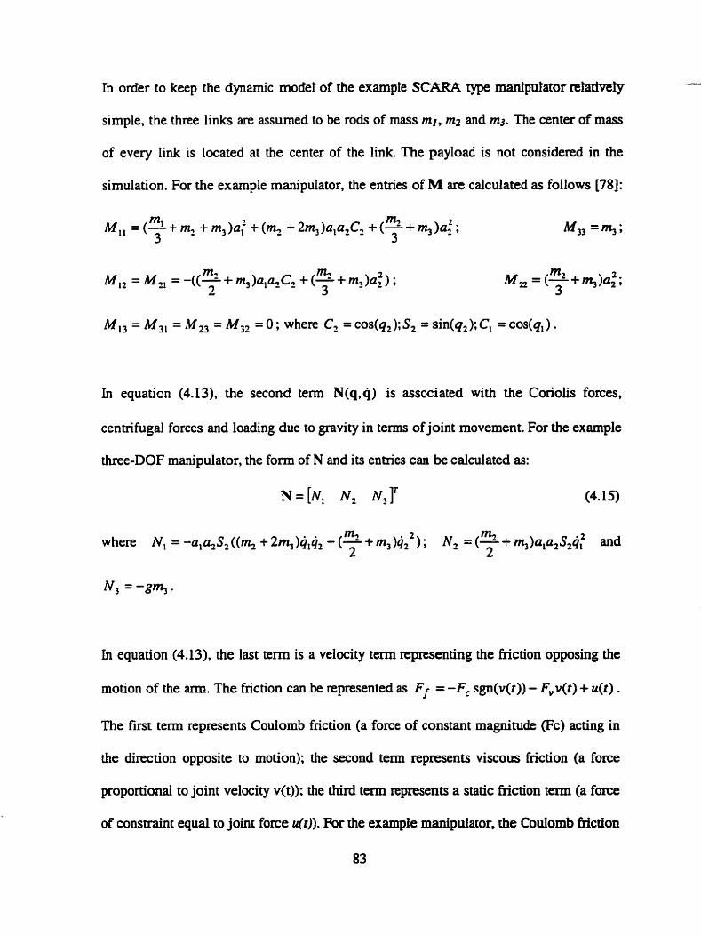
In order to keep the dynamîc mode1 of the example SCARA type rnaniprùator relaImeiy

simple, the ihree links are assumed to be rods of mass ml, m2 and m3. The center of m a s

of every link is located at the center of the link. The payload is not considered in the

simulation. For the example manipulator, the entries of M are calculated as follows [78]:

m, 2 4, = M,, = - ( ( ~ + r n , ) a , o , ~ +(-+m3)at): 3

In equation (4.13), the second term N(q,Q) is associated with the Coriolis forces,

centrifuga1 forces and loading due to gravity in terms of joint movement. For the example

three-DOF manipulator, the form of N and its entries can be calculated as:

N=[NI N2 N ~ T (4.15) - m, where N, = -ala,S2 ( (m, + 2q)4,q2 - (-2- + m,)<) ; N2 = (2- + rnJo,aJ2q; and

In equation (4.13), the last term is a velocity term representing the friction opposing the

motion of the arm. The friction cm be represented as FI = -F, sgn(v(t)) - F,v(t) + n(t) .

The first term represents Coulomb fnction (a force of constant magnitude (Fc) acting in

the direction opposite to motion); the second terni represents viscous friction (a force

propor&ional to joint velocity v(t)); the thirà tenn represents a static fiction term (a force

of constraint equal to joint force Mt)). For the exampie manipdator, the Coulomb friction

83

is considered in the following fom: F = , where bi is the coefficient

of friction for joint i. Function sgno shows that the direction of friction is opposed to the

motion generated by the actuatoa.

This dynamic model will be used for simulating the dynamic response of the robot under

the control signal. For the simulation purpose in this thesis, the inputs of the dynamic

model are torques (forces) and the outputs are joint accelerations. The joint velocities and

positions are calculated from the joint accelenitions using Euler numencal integration

method ( q, = qi-, + qi& ; qi = qi-, + qi& ; where i represents ith step and & is the step

time). The detailed parameters, such as the mass and length of a h ic , for this dynamic

mode1 will be introduced dong with the simulation results in Chapter 5.

4.4 Projection Model

Al1 of the readily available viewing technologies are 2D (monitors, printers, video and

film), even the visual cortex of human eyes is a 20 environment. In o&r to present the

images of the scenes in the simulation, a 2D representation of the 3D scenes must be

created [110]. As discussed in Chapter 3, the projection model can transform the position

information in 3D robot space into 2D image space. The type of projection model should

be selected by considering the characteristics of the observed objects and the specinc task

of the vision system. Because the top planes of the joints of the SCARA type robots are

parailel to each other, it is possible to use one camera with a scded orthogonal projection

mode1 te capture al1 the planes in one image. Sceled orrhogod projection modeC

simplifies the procedure of the image formation.

Figure 4.3 Overhead view of the example SCARA type robot.

4A.1 Projection of Joint Angles

From overhead, the ideal image of the top planes of the example three-DOF SCARA type

robot mode1 is s h o w as in Figure 4.3. The circles on the top planes can represent the

corresponding joint, which cm be considered as a cylinder. The centers of the circles are

assigned as the origins of the joint coordinate -es.

One stationary camera c m be placed overhead with the image plane parailel to the top

planes of the joints in order to obtain the images as given in Figure 4.3. If the motion

dong the direction of optic axis of the camera is rninor and can be ignoreci, then the

distance between the image plane and the top planes c m be assumed fixed whm the

robot moves in the workspace. In this situation, a scaled orthogonal mode1 can be useci.

The transformation between the robot space and the camera space can be shown as:

whcrcsis afixedsdefaaors=~;dis~~of~ctntrOiéof chtobservtdpoint

set which is located by vision system, and f is the focal iength; [u, vlT are the coordinates

of the observed points in the camera referrnce frame, which are the centers of the circles

on the top planes of the joints; [x. y]T are the coordinates of the observed origin points of

the first or the second joint frame.

In a vision system the analyzed image is usually a digital image, which is easily stored

and processed by a computer. If the digitization emor is considered, according to equation

(3.12), equation (4.16) will be:

where [I, are the digital coordinates of a point in the image plane; [la JO]' are the

digital coordinate of the center of the image plane; Au and Av represent the horizontal

and vertical sampling intervals.

According to equation (4.17), the trajectory P, of the origins of the jth (j= 1, 2) joint can

be represented as

and the projection of the trajectory in the camera plane can be shown as:

P, = P,(u,v) = P,(=,sy) (4.19)

where x, y represent the x and y coordinates of Oj ÿ=I,Z). The angles in the camera

plane, which are the results of the projection of the joint angles from the joint Caaesian

space to the carnera space, are shown in Figure 4.4. It is obvious that

86

8, =arctgf y I x ) = a r e ~ g ( s y l ~ ) = a ~ e i g f v / ~ ) = B , 4.20)

is correct if camera's x-y plane is parallel to the x-y plane of joint Cartesian space.

Equation (4.20) indicates the joint angular displacement in joint Carterian space is equal

to the angular displacement measured in the image feature space. But due to the camera

distortion and digitization enor, equation (4.20) is not held strictly. [u, vJT are actually the

analog coordinates of the image in the camera space. Usually digital coordinates [I,

are obtained directly from the cornputer image fiame. According to equation (3.12).

equation (4.20) can be changed into:

B, = arctg(v l u ) = arctg((J - J,)Av /(l - 1,)Au)

Figure 4.4 Joint angles in robot space and camera space under scaled orthogonal

projection.

For a mal camera, sampling intervals Av and Au are not equal and they are in the form

of non-linear hinctions of the coordinates [K. vJT and can be changed with tempera=

and vibration in the environment [95].

In the simulation, bv wiH be assmnect tcr k eqnat ta &r , chm 8, = &gf LU I M) wiB - - -

be held. This assumption will reduce the complications of the simulation. If the distance

between the camera and the observed objeci is fa. enough, the emr produced by this

assumption cm be ignored. Then the joint angle can be measured by

urctg((J - J O ) / ( [ - I o ) ) .

4.4.2 Projextion of Prismatic Joint

The third joint of the three-DOF SCARA type manipulator is a prismatic joint. The

position variable of the ihird joint is a linear displacement. From the side view, the ideai

image of the third joint from a camera is shown in Figure 4.5.

I

Figure 4.5 Side view of the thirci joint h m the camera.

The displacement of the prismatic joint wiU be recorded by another camera, which will

recognize a mark (shown in Figure 4.5) at the end of the joint. The opticd axis of the

camera is perpendicular to the axis of the pnsmatic joint. The mark could be a circular

iine painted around the prismatic cyünder. The vertical position of this Iine is represented

by d3, which is the third joint variable.

The projection procedure can be developed by the iollavving quaiion, whiçh. presents the

relationship between the coordinates of the observed mark in the robot space and image

featwe space:

w = SO,, = (K - KJAw (4.22)

where w are the comsponding image coordinates of the joint displacernent dong the y

axis; K is the digital coordinate of the joint displacernent in the image space; Ko is the

digital image coordinate of the origin of the image frame; Aw is the sampling intemal

dong the moving direction of the prismatic joint in the comsponding image space.

Because the image formation procedure is closely related to the physical characteristics

of the devices in a vision system it is quite difficult to simulate a real image formation

procedure. The previous projection mode1 shows the relationship between digital image

coordinates and the analog Cartesian coordinates of an observed point. Chapter 5 will

simulate the formation procedure of the digital image coordinates, which wiU be used as

the image features of an observed point.

4.5 Contrat Law

The control strategy for robots is an intensive topic in robotics research. There are

volurninous publications on the robot control theory, ranging from PD (Roportional-

Derivative) control to fuzzy connol. A control system causes the joints or the end effector

of a robot to follow a prescribed trajectory and apply the desired force or toque to an

object that is manipulated by the robot or with which the robot is in contact. PD position

control law will be simulated for the proposed direct Msual servo control system.

89

hdependent-joint PD controt [7ff is su far ttit mo~t papular feedback eon tmk for

robots. A proportional controller has the effect of nducing the rise time and will reduce,

but never eliminate, the steady-state emr. A denvative controller has the effect of

increasing the stability of the system, reducing the overshoot, and improving the transient

response. P D (Proportional-Integral-Derivative) control is also a widely used contml

method. An integral controller has the effect of eliminating the steady-state emr, but it

may make the transient response worse 111 11. The independent-joint PD control means

that every joint has an independent PD controller, which is driven by the error function of

each joint. In this case the position of every joint is measured and sent to the appropriate

PD controller. The structure of the controller is s h o w in Figure 4.6.

The advantages of using a PD contmller include: very simple to implement; suitable for

nal-time control; and the behavior of the system can be controlled by changing the

feedback gains. On the other hand, there are some disadvantages of using a PD controller

such as: it needs high update rate to achieve reasonable accuracy; there is always traàe-

off between control accuracy and the system stability; and it does not consider the

couplings of dynamics between robot ünks

In general, using a PD feedback controller with high update rates cm give an acceptable

accuracy for trajectory tracking applications. In [49], it was proved that using a linear PD

feedback law is useful for positioning and trajajectory tracking.

The desired trajectmy for the robot cm be dtscrikd by the jomt rrajcetay w the end

effector mjectory. The vision sensors may also measure the position of every joint or the

end effector. If the trajectories are given in the end effector fiame, then inverse kinematic

transformation may be necessary. Basic control structure and the corresponding formula

for different trajectones will be discussed in the following sections.

4.5.1 Independent- Joint PD Control with Known Joint Trajectory

A desired joint position q d is compared to an actual joint position q and the difference is

multiplied by a position gain to produce an output for the actuator. In order to remedy the

damping during the fast movement, a velocity referencc is often proposed, which requires

the trajectory planner to specify the desired velocity q, (as show in Figurr 4.6) (41. The

output torque can be represented as the fouowing:

t = K , e + K d è (4.23)

where position gain: K, = diag[k,, k,, k,, 1, derivative gain:

Kd =diag[kdl kd2 kd3], ermrfunction: e=q, -q,andibdenvativewithrespt

to time is e = q, - Q . Because the example manipuhtor has k e e DûF, IE, mi& & are

As mentioned in Section 4.4, the kinematic error wilI be calculateci by cornparhg the

desired and the real image feahires (here are image coordinates), so the desired trajectory

wili be projected onto the image feature space by scaled orthogonal projection, and e will

be the joint m p u k disphcement e m r (for nvdute joint) +x joint ü m displacement

eror (for prismatic joint) caiculated in image space.

Figure 4.6 Joint PD controller with a known joint trajectory. R: Robot Dynamics

45.2 PD Control with Cartesian Trajectory

The position controller discussed in Section 4.5.1 is based on the cornparison of the

desired and red joint trajectories. It is very common that the trajectory of end effector is

planned according to the task variables represented in Cartesian coordinates because the

robot task is usually performed by the end effector. In the simulation, the joint positions

are measured by the vision system directly, so the= is no sensor to measure the position

of the end effector cürectly. If the trajectory is initially specifed in tenns of the

coordinates of the end effector, then kinematic transformation is required to perform the

conversion between the displacement of the end effector in Cartesian coordinaie hime

and the rotational displacement of revolute joints or linear displacement of the prismatic

joint. The key part of this control system is still the independent-joint PD controIIer.

There are two choices to perform the control with Cartesian trajectory.

F l p 4.7 shows that the des ird Cartesian trajectory f i is cunueacd into joint

variables, and then the following control scheme is presented in Figure 4.6. The desired

and real Cartesian trajectories are xd and x , respectively. The desired and real Cartesian

velocities are x, and f , respectively. Considering the possible emr of the kinematic

model of a robot, the estimated desired joint displacement and velocity are assumed to be

a, and 4, . which are calculated by the kinematic model.

Figure 4.7 A joint PD controiler with known Cartesian trajectory. M applied to

estimate the desired joint trajectory.

M: Inverse Kinematic, R: Robot Dynamic Mode1

Figure 4.8 shows that the error between the real and desired trajectories is calculated in

terms of the Cartesian coordinates of the end effector Erame. After inverse transformation,

the error signal is input into the PD controller. Because the vision system does not

measure the position of the end effector dirrctly, it is necessary to transfomi the

measurement results obtained h m the vision system into the Cartesian end effeaor

coordinate frame. The real end effector displacement and velocity P and are

calculated by forward kinematic of the robot.

Figure 4.8 A joint PD controller with known Cartesian tmjectory. FIS applied to

estimate the real end effector trajectory.

M: Inverse Kinematic, FK: forward kinematic, R: Robot Dpamic Mode1

In the situation show in Figure 4.8, the lanematic e m r is evaluated in 3D space, so the

joint position in 3D robot space is reconstructed from the joint position in 2D image

feature space. The method presented in Fi- 4.7 c m avoid fransforming the position

information obtained from the image feature space to the robot space. Actually the '*off-

iine teaching" procedure cm measuring joint motions directly by vision and saving for

reference joint trajectory even if the desired trajectory in robot space is aven in Cartesian

coordinates. Thus the desireci joint rrajectory can be obtained withom inverse bernatic

transformation and projection transformation of the end effector trajectory.

4.6 Summary

In this chapter, a direct visual servo control method for a three-DOF SCARA type

manipulator was proposed With the third revolute joint king fixed, the SCARA robot is

simplified to be a three-DOF manipdator with two revolute joints and one prismatic

joint. me kinematic h-misformatio~ was devefoped ixxof&ng €0 Bs peremetea. Thc

joints and links were represented as rods with mass at the centroid of each rod The

Lagrange-Euler method was used to develop the dynamic mode1 of the manipulator.

Vision-assisted kinematic error estimation was used to obtain the joint position emr.

With the proposed camera placements, the scaled orthogonal projection mode1 can

simulate the projection procedure from the 3D space to the image coordinate frame.

Digitization was also discussed when modeling the digital image coordinates.

The control errors are calculated in image coordinates and an independent PD control

rnethod was used. For the future work of this project, two kinds of image feature

recognition methods were also intmduced.

These models will be used to investigate the feasibiiity of the vision-assisteci kinematic

error estimation for a direct visual servo control method to control the example

manipulator to perform the desired trajectones. Simulation results will be discussed in the

next chapter.

Chapter 5

Simulation of a Direct Visual Servo Control Method for a

Three-DOF SCARA Type Manipulator

5.1 Introduction

In Chapter 4, a direct visual servo control method for a three-DOF SCARA type robot

was introduced. Based on the proposed method, different simulation scenanos wiII be

investigated and the feasibility of implementing an image-based visuai servo joint control

system for a three-DOF SCARA type manipulator will be discussed. The main concem is

to investigate the capability of the proposed method to track specific trajectones. Two

categories of trajectories, known trajectones of the joints and hown trajectories of the

end effector (the endpoint of the third joint), are considered. As discussed in Chapter 4,

the error signals are calculated in the image featwe space. In this simulation the image

feanires are the image coordinates of the points in an image. That means the required and

real trajectories are al1 transformed into the image space and represented in terms of the

image coordinates of the origin of the correspondingioint coordinate fnune.

In order to test the method, several e m r models are intmduced to the simulation process

and the results are analyzed These e m s include robot iink length enors, image

coordinate errors, and robot dynamic disturbances. In a practical application, every joint

actuator has a limited velocity and allowable output forceltorque. These limits codd

influence the ability of the robot to reach the required trajectory and could make the

system unstable. This chapter will alsa investigate the simulations with velocity and

forceltorque limits.

The simulation program is developed using Matlab. The flow chart and the function of

the program will be introduced in this chapter. The corresponding panuneters for the

simulation are also detailed in this chapter.

5.2 Basic Parameters for the Models

The proposed visual servo control rnethod for the three-DOF SCARA type manipulator is

composed of the manipulator model (including kinematic and dynamic parts), projection

model and control model. In this section, the parameten of models will be introduced,

which are used in the simulations presented in Section 5.5. Some panuneters will be

intmduced with specific simulation results.

5.2.1 Parameters of Manipulator

Table 5.1 D-H parameters and mass of the example three-DOF manipulator.

The zem confi~guration of the modeled three-DOF example manipulator is shown in

Figure 4.2. The numerical values of the robot kinematic parameters with D-H parameters

are listed in Table 5.1. The dynamic mode1 was discussed in Section 4.3. The m a s of the

tinks for the simulation is dso s h m in Table 5.h Ttit tmk masses mc? Link lm@s sn

roughly chosen or calculated according to the manual of Adept One robot.

The Coulomb friction F is considered as F =

simulation. The magnitude of fiction force is taken to be about 10% of the average joint

force or torque.

5.2.2 Parameters for Projection Model

One camcra is placed overhead so that the image plane of the camera is paralle1 to the top

planes of the joints in order to obtain the image as shown in Figure 4.3. In the simulation,

the distance between the image plane of the camera and the observed plane of the fint

two joints is assigned to be 1 m. The second camera is placed beside the third joint so that

the optical axis of the camem is perpendicular to the axis of the pnsmatic joint. The

distance between the image plane of the second camera and the axis of the pnsmatic joint

is assigned to be 0.5 m. Depending on particular applications. these distances can be

obtained from camera calibration. In the simulation, the image precision is assumcd to be

0.00 1 mfpixel for the first camera and 0.0005 m/pixel for the second camera.

As discussed in Chapter 4, scded orthogonal projection mode1 is used to simulate the

transformation between the 3D coordinates and the 2D image coordinates of the observed

points. The digi tization transforms the image analog coordinates into digital coordinates.

The PD control method is applied to the joint contmller. The control parameters are nuied

by trial-and-error so that the joint displacement errors can be controlled in a small range

and the joint output torquedforce can be reasonable. Generally, the robot trajectory is a

combination of different curves. It is not easy to dynamically identiw the transition points

among different curves and assign different control gains accordingly. Therefore it is

very helpful if the same control gains could be used for al1 the curves. Extensive test nuis

were performed by trial-and-enor to tune the control parameters such that a unique set of

gains could be used for most caseslajectories. As the tuning result, the conml

parameters for different cases are taken the same (K, = [4000 3000 200001~ and & =

1100 100 2001T) if not specified These numbered values are about the same order of

magnitude as that in Schilling [72]. The units of the proportional gains are N/m (for

prismatic joint) or N &ad (for revolute joints). The units of the derivative gains are N

dm (for prismatic joint) or N m s/rad (for prismatic joint).

The joint velocities and force/torque are assigned according to the specifications of some

commercial robots. In Section 5.5.5, the allowable joint velocities and forcdtorque will

be introduced and their effects will be investigated.

5.3 Prescribed Trajectories

In this section, two types of trajectories are discussed The combination of these

trajectories can simulate more complicaied tracking tasks for the robot.

This type of trajectory is described in the joint space and represented by the joint

variables, and the actual joint trajectory cm be compared with the desired joint tmjectory.

The fiat case for tracking the known joint trajectories (referred to be T W l in the

following discussions) requires every joint move with a constant angular velocity (for the

revolute joints) and constant linear velocity (for the prismatic joint). The desired

trajectory is represented by the following expressions: q, = yt; q, = w2t; q, = v,t. The

numericd values of the angular velocities oi and 02 of the two revolute joints (fmt two

joints) and the linear velocity y of the prismatic joint (third joint) will be assigned with -

the specific simulation results.

The second case for tracking the known joint trajectories (referred to be W 2 in the

following discussions) is that the joint displacements are expnssed as a harmonic

function q, = A, (1 - cos(il,t)) ; q, = a(l- cos(gt)) and q, = d, - A=, cos(%t -xi21 ,

where Al and A2 are the maximum angular displacement of the first and second joints, A3

is the maximum swke of the prismatic joint, q is the angular frequency of the cosine

function (i = 1, 2. 3). Then the joint velocities cm be calculated as ql = qqlsin(qlr) ;

49 - = 4q2sin(q2t) m d q3 = qqisin(q3t - n12) . If the amplitudes of the velocities are

taken to be ml, y and v3 as used in the fint case, then A, = a>, 1 ql 1,; 4 = a>, 111, and

A, = v, I q3. When qi reduces, the fÎequency of the cosine function will be reduced.

This type of trajectory is defined by the trajectory of the end effector in the Cartesian

world coordinate frarne. Because the vision system measures the joint tmjectones in

terms of the image coordinates, the measured joint trajectories by vision system cannot be

compared with the desired tmjectory directly. The desired end effector trajectory should

be transfotmed into joint frame by inverse kinematics.

The third expected trajectory is defined in tem of end effector mjectory (referred to be

W 3 in the following discussions) that requires the end point of the third joint move

along a spiral cuve where the projection of the curve ont0 the xoyo plane is a circle and

the prismatic joint rnoves along a axis (the axis of the pnsmatic joint). The desired

trajectory can be expressed as x, = a, + (a, /2)(l+ cos(a>,t)) ; y, = (a, 1 2) sin@$)

and 2, = dl T v3r ; where is the angular velocity of the end point when moving dong

the circle. Obviously (x, - (a, + a, 12))' + y: = (a, /2)* guarantees that the projection of

the curve ont0 the xozo plane is a circle with a radius of a, / 2 centered at [al + a, 1 2, O].

5.4 Simulation Program Flow Chart

The simulation prograrns are developed in MatLab. The program has a function option

menu, which is easy to be used for the simulations inaoduced in this chapter. The

program flow chart in Figure 5.1 shows the functions of the simulation program, which

include:

a Setdon of the demPd trajedoqr The osrrcarr sekt fourctiffercnt asjtctorics

as discussed in Section 5.3 in an option menu. Joint trajectories are given in t e m of joint

variables. End point trajectories are given in terms of Cartesian coordinates.

O Simulation of the kinematic, dynamic and projection models. This is the main

part of the simulation. The kinematic, dynamic and projection models are based on the

discussions in Chapter 4. Kinematic and dynamic models simulate the robot motion and

the response to the contmi signal. The projection rnodel simulates the fomation of the

image features in terms of image digital coordinates.

O S e l d o n of the error for khematic, dynamic and projection models: The

program can sirnulate the results with link length errors, dynarnic error and image

coordinate errors introduced into the comsponding models.

O Simulation of the control model: The PD control mode1 has two control

parameter vectors, which are proportional to the position gains and derivative gains.

These parameters cm be tuned b y trial and error according to the simulation results.

a Plot of the trajectory: The desired trajectory and real trajectory can be plotted on

the same graph so that the performance of the point-to-point tracking cm be compared

Rot of the errors of the joint rnovement: These Rsalts hdicate the tradairg

performance at each interval, which can supply dues for adjusting the control parameters.

Plot of the actual velocity, acceleration and forcekorque of joints: These

curves of the dynamic performance couid supply compxehensive evaluation of the

tracking performance thou the purpose of the simulation is to obtain reasonable

displacement tracking performance,

l P given joint trajectory given end-point trajectory

plot graphs .

desired joint /I kinematic kinematic displacements \I mode14 errot

image feature projection

projection Cl

dynamic

simulated joint variables

1 kinematic 1 model hP

Figure 5.1 The 80w chart of the simulation program.

This section will present various simulation results to analyze the performance of the

suggested visual servo method. The main concem is the tracking performance, which is

presented by the displacement errors of the first, second and third joints between the real

trajectories and the desired trajectories. The actual velocity, acceleration and torqudforce

of each joint are also investigated for various cases and presented for some cases. Euler

numerical integration method is used. The simulation time is assigned to be 8 seconds.

Uniess otherwise specified, the step time for the numerical calculation is 0.1 m. The step

time is chosen such that the system output can be stable. In Section 5.5.1, the effect of the

step time is also investigated and some results are presented.

5.5.1 Simulation Results with no Error Input

This section analyzes the simulation results with no enor input, i.e., there is no kinematic

emr , image coordinate erron and dynarnic disturbance during the simulations.

Figure 5.24 shows the tracking performance of TRAI1, The two revolute joints

velocities are desired to be oi = = 1 rads, while the prismatic joint velocity is desired

to be v3 = 0.1 d s . The prismatic joint will move upward by 0.2 m and then wiIl change

the direction to move downward. Figures 5.2-l(a) shows the desired and real trajecton

of the endpoint of the third joint. The two trajectories cannot be differentiated because the

e m r of the trajectory is very small and the scale is limited Figures 5.2-1@) and 5.2-l(c)

show the desired and reai trajectories of the origins of the first and second joints,

rcspmively. Figures 5.2- 1 (d) md 5. %Ife) show that dispi~eement emis of ths &w - ---

revolute joints are less than 0.003 rad. Figure 5.2-l(f) shows that the displacement error

of the third joint is limited between -1.5mm and -1 mm. Figure 5.2-2 shows the actual

velocity, acceleration and forcdtorque during the simulation. The average values are in a

reasonable range (except that the spike in Figure 5.2-2(e) is -36 rads2 and the spike in

Figure 5.2-2(h) is S667 Nm).

In the case shown in Figures 5.2-3 and 5.2-4, the robot is required to perform the same

movement as in Figures 5.2-1 and 5.2-2, but the step time for the simulation is changed

from 0.1 ms to 0.08 ms. Except for the initiai spikes in Figures 5.2-l(e) and 5.2-2@), the

other spikes produced by digitization disappear. In applications, the initial spikes could

be reduced by special design of the initial path to reach a stable motion. A more criticai

situation for a robot is that the robot is required to start as quick as possible without initial

path planning. If the robot can go to stable state shortly, then the robot behavior will be

better when a suitable initial path planning is available.

F Ï p 5.2-5 shows the influence of imege resdution. Here every pixel in the hege

represents 2 mm in 3D space. There are more spikes on the curve of the acceleration and

torque output in Figures 5.2-5 (d-h) than in Figure 5.2-2. The results in Figure 5.2-4 and

5.2-5 reflect that the spikes are produced not by the movement states of the joints. These

spikes could be reduced by adjusting the numerical algorithm or parameters. Sharp

changes in velocity (either value or direction) such as those happen in initiai tirne, are

another source for the spikes. The effect of these spikes is discussed in Section 5.5.6.

In Figure 5.2-6 ihe~e i s no frithn tem in the simulate& Qynamic -1. Ths d g . . . - . - - - -

show that the effects of digitization are more obvious. The possible reason is that the

friction in Figure 5.2-1 becomes a damping factor that reduces the effects of digitization.

The average displacement error of the third joint that is shown in Figure 5.2-6(f) is close

to -1 m.

Figure 5.3 shows the tracking performance with TRAJZ. The desired maximum velocities

of the two revolute joints are assigned to be 1 rads and the desired maximum velocity of

the prismatic joint is assigned to be 0.1 mis. Compared with Figure 5.2-1, there is more

fluctuation on the c w e shown in Figure 5.3. change of the velocity causes these

fluctuations. When the frequency of the cosine lunction, which describes the

displacement of each joint, reduces, the magnitude and frequency of the output reduce

too. On the other hand, if the changes are very dramatic, the response time may be longer

for the system to reach a stable state. Because the robot joints are started harmonically,

the initial fluctuation is not as serious as those cases for TRAJ1 and W 2 .

Figure 5.4-1 shows the tracking perfonnance with TRAJ3. The endpoint of the third joint

is required to move dong a circle with a constant velocity (W2 radls) in a plane pardel

to plane x3y3 while it moves dong the 23 axis with a constant velocity (0.1 ds). In 8

seconds, the end ef5ector performs two cycles that means it will draw two circles and the

prismatic joint will move downward and upward twice. The spiral movement of the end

effector should be transformed to the joint space by inverse kinematic transformation,

and then projected into the image space. The PD control parameters are assigned the

same as TRAJl and TRAJ2 cases The dispiacement ecrors of the two cevolute joints are

between kû.0024 rad. The displacement error of the pnsmatic joint is between -1.5 mm

and -1 mm.

By adjusting the control parameters of the joint controllers, the average error cm be

further reduced. Figure 5.4-2 shows the same simulation result as that in Figure 5.4-1

except that the parameters of the joint controllers have been changed to 4 = [20000

5000 20000]~; & = [100 150 5001T. Obviously the output c w e of displacement emrs

are better than that in the simulation of Figure 5.4-1. The results of other cases cm also

be improved by adjusting the control panuneters.

In Figures 5.2-1 (0, 5.3(f), 5.4- 1 (f) and 5.4-2(f), the maximum emrs of the third joint

displacements are al1 multiplied by 0.5 mm. Actually every pixel in an image of the third

joint represents 0.5 mm, so after digitization, the maximum emr of the third joint is

always the multiple of 0.5 mm. This phenornenon proves the influence of the digitization.

In TRkll and TRAJ3 cases. the third joint is reqyired to move at a constant velocity.

However in TRAJZ case, the third joint is required to move at a variable velocity,

therefore there are more fluctuation on the output as s h o w in Figure 5.3.

The previous results show that the static displacement emrs of the third joint are more

stable than the displacement emrs of the other joints. The first two rotary joint

displacements are in t e m of the angles in image space, which rn calculateci by

arctangent function of the digital coordinates dong tuw image coordinate axes The

coordinate of the third joint is the digital coordinate dong one image coordinate axis.

Thqs more digitization enon are produced than the calculation of the linear displacement

of the third joint.

TRAJ1, 2 and 3 are based on the link masses of 10 kg for the first link, 5 kg for the

second link and 2.5 kg for the third link, respectively. The order of magnitude of these

masses is the same as that in Schilling [72]. As this mass was too large for the slender bar

assumption, the masses of links 1, 2, 3 were reduced to be 1 kg, 0.8 kg and 0.5 kg, and

the results of simulation are included as TRAJ3 with adjusted mass case as shown in

Figure 5.5. The magnitudes of friction force are changed to be 0.2 N m, 0.2 N m and 0.8

N for the three joints, respectively. Because of reduced inertia of each iink, the control

gains iue reduced as well, which are & = 1600 600 60001T and & = [60 50 100~~.

5.5.2 Simulation Results with Image Coordinate Error

This section will analyze the simulation results with image coordinate emrs. Because it

is not easy to simulate various emon in a vision system, the image coordinate emrs can

be considered as the comprehensive results of the lens emrs, the projection mode1 emrs

and the errors generated during image processing procedure. During the simulation, the

image coordinate errors are represented by the value of sarnpling error (dp ixe1) in an

image and produced by a randorn f'unction with a nomial disaibution. The maximum

error is assigned to be 0.5 rndpixel.

Figure 5.6-2 TRAJ3 with adjusted mass and random image coordinate emr: (a) trajectory of end point, @) and (c) trajectones of first and second joints, (d) to (f) joint displacement eifors.

Figure 5.6-1 shows the tracking performances when the robot is required to ûzck TRA13

and image coordinate errors are produced randomly. The comsponding kinematic and

control parameten are assigned to be the same as those in Figure 5.4-1 in order to

observe the differences between the results with random image coordinate emrs and the

results without image coordinate errors. In Figure 5.6-2. the masses of links are reduced

as in Figure 5.5. The control parameters in Figure 5.6-2 are dso the same as those in

Figure 5.5. The other trajectories are dso simulated but due to space limitations are not

shown here. A11 the results show that image coordinate emrs generate more digital noise

on the output cwes. By adjusting the control parameters and robot joint velocities, the

average error and the frequency of the fluctuation can be reduced.

5.5.3 Simulation Results with Dynamic Disturbance

This section will analyze the simulation results with dynamic disturbances. Dynamic

disnubance is simulated as the forces or toques of the joints and represented by a cosine

function. r,,, = [50 50 50r cos(5t) in N (for prismatic joint) or N m (for revolute

joint). The dynamic disturbance c m be thought as the comprehensive simulation resuits

of the disturbances produced by the robot itself andlor the environment. The source of

disturbance might be vibration, irnbalance distribution of mass. electrical disturbance, etc.

In a practical situation the dynamic disturbance would be a cosine function with a d t i

frequency and amplitude.

Figure 5.7-1 shows the tracking performance with TRAJ3 and dynamic disturbance. The

control gains in Figure 5.7- 1 are I(, = 11200 1600 400001~ and I(a = [50 80 ZOO]. The

figute shows that the eRict of the dynamic disturbmce is much stronger ttran that of&=

digitization e m r , even though the frequency of the fluctuation is lower than that in the

case with image coordinate enors show in Figure 5.6-1.

In Figure 5.7-2 the masses of Links are reduced as in Figure 5.5. The expected tmjectory

is TRAJ3 as well. Dynamic disturbance is represented by a function

tdirrvn = [5 S 5r cos(%) in N (for prismatic joint) or N m (for revolute joint). The

control gains are IC, = [ 1 6 0 1600 60001T and &= (50 50 100IT.

5.5.4 Simulation Results with Link Length Error

The link Iength erroa may corne from various sources, such as the manufacturïng emrs,

link defornation, mechanical Wear, transmission and backlash, etc. Instead of choosing

some specid e m r models, this section will consider the link length emrs as random

enors with a nomal distribution. The comsponding kinematic and control parameters

are assigned to be the same as those in Section 5.5.1 in order to observe the differences

between the results with link errors and the results without link erron. The maximum hnk

emor is assmed to be 0.002 m.

Figure 5.8- 1 shows the displacement mcking performances with T W 3 and link mors.

The figures show that the iink hgth emm have strong effects on the first two joints. The

amplitude of the joint displacement error is similar to the prevîous simulation cases. The

third joint displacement e m n in the entire four situations are between -1.5 mm and

In order to observe the effect of link Iength errors clearly, the coordinate emrs of Oi and

Oz have been s h o w in Figure 5.8-2. In Figure 5.8-2, the effect of Link emrs is more

obvious. The introduction of the link enors enlarges the erroa dong the coordinate axes.

When the link length changes during the robot movement, the controi emn in terms of

the errors between the desired and actuai image coordinates will be influenced. The

controller cannot figure out the source of this error and simply adjusts the joint

torquelforce to reduce the control emrs that are produced by iink length emrs. This

behavior may produce more errors due to joint movement.

In Figure 5.9-1 and 5.9-2 the masses of links are reduced as in Figure 5.5. The expected

trajectory is TRAJ3. The control parameters are the same as in Figure 5.5. The input link

emn are the same as in Figure 5.8-1. The results show that displacement errors of the

revolute joints are in the same range as in Figure 5.5 and the displacement emrs of the

third joint are between -1 mm to 4.5 mm.

5.5.5 Simulation Results with Joint Velocity Limits

The previous simulations al1 required that the joint velocities be much smaller than the

maximum velocities the joints can achieve and no velocity limit was set during the

simulation. In this section the desired joint velocities are assigned to be close to the

maximum velocities in order to observe the tracking perfo~mance of the suggested

method at maximum joint vehcities. According io the specifications of some commefciaf

robots, the maximum velocity lirnits for this simulation are chosen to be q, = & = 6

rack and v3- = 5 1x11s.

In Figure 5.10, the expected trajectory is TRAJJ and the desired velocities of the first two

joints are 1 .Sn rad/s. The desired veloci ty of the third joint is 1 m/s. Even &ter adjusting

the control parameters, the emor output and the frequency of the fluctuation are still much

higher than that in Figure 5.5-1. The PD control parameters are &,=[15000 15000

20000jT; &=[lO 10 1001' This result shows that higher velocity triggers higher

digitization emrs during image processing. The desired joint velocities should be

designed relatively lower than the maximum velocity.

5.5.6 Simulation Results with forqueForce Limits

In an actual environment, the joint actuators (motors or cylinders) have limited power

that may not provide enough acceleration in order to follow the desired trajectory at the

corresponding velocity. This practical limitation may produce strong fluctuations of the

output torquefforce when dramatic changes of the velocities are required-

According to the data of some commercial robots, in the simulation the maximum toques

for the fmt two revolute joints are assumed to be 100 Nm while the maximum force for

the prismatic joint is assumed to be 100 N. The following figures show the simulation

results for the different desired tnjectories. There is no kinematic, dynamic or image

coordinate e m r in the following simulations. The kinematic and control parameters are

assigned to ùe the s a m t as hose in Section 5.5.1 in orda io observe the

between the results with and without forcdtorque limits.

Figure 5.11-1 shows the tracking perfomance with TRAJI. Because of the limited

torques of the first two joints, it takes about 2.5 sec for the actual joint movement to

approach the desired state. The maximum displacement errors for the fint and second

joints are 0.02 rad and 0.008 rad, respective1 y. These errors are both produced during the

initial penod. For the third joint, there is stronger fluctuation when the joint changes its

direction of motion.

By adjusting the control parameten, the tracking performance can be improved Figure

5.1 1-2 shows the simulation results when the control parameters are changed to be &, =

[50000 20000 25000]' and Kd = [150 150 3001T. The initial time of the first joint is

reduced to be 1- 1.5 sec. After that the displacement erron are limited beh~een M.003

rad. For the second joint, the initial time and the amplitude of the fluctuation are both

reduced. For the third joint, the response to the change of the velocity is faster than in

Figure 5.11-1.

The other cases with TRAJ2, TRAJ3 and TRAJ3 with adjusted masses are also

simulated. Ail the results prove that the suggested servo control system can be convergent

but the= is not a universal set of conml parameters that can be used in al l the situations.

Figure 5.1 1-2 TRN l with force limits after adjusting the control parameters. (a) trajectory of end point, @) and (c) trajectofies of first and second joints, (d) to ( f ) joint displacement emrs.

Based on the robot kinematic and dynamic models. projection model and control model

presented in Chapter 4. a three-DOF SCARA type manipulator with a visual servo

conwl system has k e n simulated in this Chapter. The control error is obtained by

cornparing the desired and acnial digital image coordinates, which are calculated by the

scaled orthogonal projection model. A PD joint controller was simulated to investigate

the tracking performance (displacement errors) of the robot. The trajectories of the robot

include two categories, known joint trajectories and known end effector trajectories

where the joint trajectories are calculated by invrrw kinematics.

Generally speaking, the outputs show strong digital noises. Meastuement emrs of image

coordinates have strong effects on the output when they are produced randomly in every

step of the whole simulation procedure. D ynamic disturbances as additional

torques/forces to the joint are simulated as a hannonic function. According to the

simulation results, dynamic disturbances might have stronger effects on the outputs than

the image coordinate e m a . The errors of the link lengths increase the displacernent

errors but could be controlled in an acceptable range.

The response is also investigated when the system cannot provide enough power to meet

the acceleration requirement. The results show that the system is convergent.

No cornparison was made with published data, as to the best knowledge of the author,

there is no work on visual servo control of a SCARA robot. However, extensive test runs

for different cases were performed (most incïuded in the thesis) to make sure the program

was correct and the results were vaiidated. The simulation results demonsirated that

vision-assisted robot kinematic error estimation could be used in a visual servo control

system for a three-DOF SCARA type manipulator.

Chapter 6

Discussion: Vision-Assisted Robot Kinematic Error

Estimation in a Fault Tolerance Robot

6.1 Introduction

Robot vision technology has become one of the most popular topics in robotics research.

Besides the studies on the humanhimai vision with the goal of understanding the

operation of biological vision systems, robot vision researchers stress on developing

vision systerns that are able to narigate, recognize, track objects and estimate their speed

and direction.

The vision application mode1 introduced in Chapter 2 shows the basic structure and the

information flow among different function modules. Generally, the vision system could

answer two questions: "What it is" and "Where it is" (621. These two questions are also

the standards for categorizing the vision applications. A practical robot vision system

could answer both questions, but often focuses on one of them. One of the important

steps in a vision application is how to make decisions based on the information obtained

from the vision system.

Vision-assisted robot kinematic emr estimation reaIizes the kinematic error estimation

based on the "where it is" information obtained h m the vision system. A dKea visual

servo control system for a SCARA type manipulator discussed in Chapters 4 and 5 is a

typicd appficatim of visim-assisteck robot kRrematic em>r estimation. The smmfmion

results demonstrate that it is feasible to form a visual servo control system with the joint

position error estimation in the image feature space. For the SCARA type manipulator,

the features could be the image coordinates of the special geometrical feiiture points of

the joints.

A new robot can always obtain fault tolerant capability h m special considerations

during the design procedure. However for an existing robot it is quite difficult to improve

its fault tolerance performance without structure changes. The direct visual servo control

rnethod currently could not replace the traditional robot control system due to the

shortcomings of the vision system, but it could be an alternative choice when some

senson fail. Furthemore because a vision system can flexibly and extensively collect the

information in the robot workspace, it cm perfonn high-level analysis of the joint

movements to make decisions as well as low-level servo control to fulfill requested tasks.

The interesting point is that drarnatic stmcture changes are not necessary for an existing

robot to improve its fadt tolerance by employing a vision system. As a case study of this

chapter, the vision system is required to replace a failed joint sensor of a threeDOF

SCARA manipulator so that the robot can follow a fidl or a partial recovery scheme.

Currenily there is no universal method for implementing robot vision application. The

selectiun of the feanires and the placement of the cametas are both dependant on the

actual robot task and the specific structure of the robot. At the end of this chapter, a

pssibie methad to m m the joint positions of a PUMA type maniputatm with e vision

system will be discussed.

6.2 Application in Fault Tolerance System

The essence of the vision-assisted kinematic emor estimation discussed in the previous

chapters is to measure the joint positions with a vision system. Cumntly the joint sensor-

based servo control technology is still the paramount choice in an industrial environment

because the rd-time response, accuracy and reliability of the traditional control system

are still better than a vision-based servo control method. However the flexibility and

broad view of a vision system contribute to the unique advantages in sorne applications.

The following sections will discuss the possible roles that a vision system can play in a

fault tolerant robot.

A robot is a rnix of mechanical, electrical and electronic components. The situation is

compounded by the fact that robot systerns are highly dynamic, resulting in very rapid

and wild responses of robots to subsystem failure [101]. Robots are king more

frequently utilized in inaccessible or hazardous environments to alleviate some of the

nsks involved in sending humans to perform the tash and to decrease the time and

expense. However, the dangerous, long distance nahm of these environs also makes it

difficult, if not impossible, to send humans to repair a faulty robot. Typically human

operaton are integral in monitoring such a system for problems, but they are not

completely reliable in detecting failures. The robots need to independently detect and

isolate internai failures and utiiize the remaining functiond capabilities to automatically

overcome the limitations imposed by the failures. If robots could be provided with

autonomous fault tolerance without requinng immediate human intervention for every

fai l u e situation their working life can be lengthened [99].

Figure 6.1: Vision system in a robot fault tolerance system.

-

To develop and realue a trdy fault tolerance system, many issues including mechanical

design, redundancy management, fault detection, system reconfiguration and recovery,

intelligent decision-making, real time control, operational software and task prioritizatioa

must be taken into consideration and stuclied. Fault tolerant control of a robot system cm

be divided into three layers: a continuous servo layer, an interface monitor layer, and a

discrete supervisor Iayer [99].

Process for controller b Sem tayer -

The vision-assisted kinematic error estimation can improve the performance of an

existing robot besides forming a visual servo control system. The discussion in the

following sections shows that a vision system can play a role in ai l the three be l s of the

-

+- Robot and Environment

P m for Interface fauit check W'3r

Image Process for Supervlsor safe check LaFr

+

robot fanit tolerant system as shown in Figure 6. t. Thepint sensor-baJ& eontrot system . A

lacks these comprehensive functions.

6.2.1 Servo Layer

Servo layer consists of the normal robot controller and the robot. In this layer fault

tolerance requires the controller to control the robot movement when a failure happens.

Usually an alternative controller must be installed for the robot. The alternative controller

cm be a totally new controller or a special control scheme for the same controiler. The

alternative controller must allow the robot to resume performing its tasks (full recovery)

or to gracefully degrade (partial recovery) if a failure is detected. One important type of

this kind of failure is sensor failure. Traditionally redundant sensors are used to increase

the fault tolerance capability of the sensor-based controller. As will be discussed in the

following sections, a vision system not only can work as a sensor to measure the

positions of some joints of a robot, estimate the kinematic error and form a visual control

system, but also can help with the failure detection of the robot. Through some special

processing on the image, the vision system cm even rneasure the velocity of the observed

object, which means one camera c m huiction as both position and velocity sensor at the

same time.

The previous chapter discussed a direct visual servo control method for a SCARA type

manipulator, which proved that the vision system could replace the traditional joint

sensors when some or ail of them have failed. The main weakness of the vision system

cornes from the computing load of the image processing. Currently the measmment

accuracy of a vision system stiH b i t s the appKcatim of a M m system ta be d as a

normal position sensor. However, when some failures happen, the accuracy and fast

response of the control system may not be very important in some situations. A safe path

planning can be designed so that the trajectory and the velocities of the joints are suitable

for the vision system. Figure 6.2 shows that a vision system can perfom different

commands given fiom the higher layer to recover the robot h m a failure state.

Depending on the robot task, the vision system can replace some of the joint sensors to

form a multi-sensor control system to perform some special tasks.

Figure 6.2: Vision system in the servo layer of a fault tolerance robot system.

Case Study

The following paragraphs will discuss a case study to demonstrate the functions of a

vision system at the servo Ievel of the robot fault tolerance system. The simulations

demonstrate that the vision system can replace the failed joint sensors to recover the robot

task completely or partidly. A three-DOF SCARA type manipulator with the saw

configuration as ttiat in Chapter 4 ancf 5 is us& in the simd*. H o w m , it is asseme& --

that the traditional joint sensors are used to supply information for the PD controller

duxing the normal operation. At some time, which is input by the user, the second joint

sensor is assumed to fail and the task manager requires the vision system replace the

second joint sensor. Now the position information of the second joint is supplied by the

vision system and the position information of the remaining joints is stiil supplied by the

traditional joint sensors. With the mixed sensor control system the robot is required to

achieve full recovery scheme (in Figure 6.3-2) or partial recovery scheme (in Figure 6.4-

2) in the simulation.

The full recovery procedure requires that the mixed sensor control system finish the

cumnt task after the information from the failed sensors is replaced by the information

from the vision system. The partial recovery scheme requires that the mixed sensor

control system reduce the velocity of each joint harmonically to zero after the

infurnation from the failed joint sensor is replaced by the information h m the vision

system. In both schemes, the transitions are assumed to be immediate and seamIess,

which means the vision servo conttoUer is dways feady ta w&

The simulation program pennits the user to input the failure time. Before a failure

happens, joint sensors measure ail the joint positions and the control emrs are caicuiated

in the 3D space. After the failure of second joint happens, the joint position of the sccond

joint is measured by the vision system, and the remaining joint positions are still

measured by the original joint sensors. When calculating the control exmr of the second

joint, the desired and actuai joint trajectories are both represented in the image coordinate - A

frame after the failure happens. In the full recovery scheme, the desired trajectory is kept

to be the original one. In partial recovery scheme, the desired trajectory is changed to be

TRAJ2 (refer to Figure 5.3) with the amplitude of the velocity equal to the velocity at the

failure time. When the velocity of a joint is reduced to 0.001 rack (for the revolute joint)

or 0.001 m/s (for the pnsmatic joint), the control system wili stop the joint.

Figure 6.3-1 shows the simulation results without full recovery scheme. In this simulation

the task requires the end point of the third joint move dong a spiral curve (cded TRAJ3

in Chapters 4 and 5) with control gains as &,=[20000 5000 2 0 0 0 0 ~ ~ and &=[IO 150

5001'. Origindly dl the joint displacements are measured by joint sensors. At thne 1.5

sec the controller cannot receive response from the sensor of the second joint. The results

show that the robot lost control and cannot hilfill the original task. Figure 6.3-2 shows the

simulation results with full recovery scheme. The sensor of the second joint is failed and

replaced by the vision system at time 1.5 sec, the mixed sensor control system is nquked

to finish the current task. The transition is assumed to be smooth and the comsponding

controt parameters are not changed. Arrordmg to the d t s , thm are some spikm with

the angular errors of the second joint that also influence the output of the first joint.

Adjusting the control parameters can M e r improve the results. The joint displacement

emor of the third joint shown in Figure 6.3-2(f) is smaller than that in figure 5.4-2(f), in

which al1 the joint position are measured by vision system. This simulation shows that the

original task can be fulfilied even though the control performance is degraded afta the

sensor of the second joint is replaced.

Figure 6.44 shows tht sirnatation resnits wittiout pmtist m v c r y sckxm. hr this

simulation the task requires every joint to move with constant angular velocity (for

rewolute joints) and constant iinear velocity (for the prismatic joint). This trajectory is

called T W l (refer to Section 5.3.1) and its parameters are the same as the trajectory

shown in Figure 5.2-1, except for the assigned original angular velocities of the fmt and

second joints are 4 rack instead of 1 rads while the control parameters are assigned to be

Kp=[300ûû 35000 700001~ and &=[200 200 5001T. Again dl the joint displacements are

measured originally by joint sensors. The sensor of the second joint is failed and the task

manager requires the robot stop every joint immediately. The resuits show that it is quite

difficult to stop the robot when it moves at a high speed. Figure 6.4-2 shows the

simulation results of the partial recovery scheme. The mixed sensor control system is

required to reduce the velocity of each joint hannonically to zero. The transition is

assumed to be smooth and the correspondhg control parameters are not changed. The

velocity output after 2.5 sec shows a smooth velocity reducing procedure even though

there are some spikes with the displacement and torque output of the second joint. This

simulation shows that it is possible to stop the robot graceNly by the mixed sensor based

controller when the sensor failure happe= This partial recovery process uui avoid

damage caused by the sharp braking of the joint actuators.

6.22 Interface Layer

The interface layer contains the tmjectory planner and provides fault detection and some

basic tolerance functions for the system. The fault detection routines continually monitor

the state of the robot in order to catch any failures in the system. The joint sensors can

mfy obtaiir the rotary or hmr dispi-t of a jomt k is diffieutt tv measurr thejoint

position in the world space with an intemal sensor. However the vision measurement has

the ability to perform a nonîontact measurement. Therefore the vision system cm be

used as a redundant sensor to check the actual position of the joints and end effector in

the world space. The joint displacements in the corresponding joint frame can be

calculated from the position descn'bed in the world m e , and compared with the output

of the joint senson. The actual joint trajectories in the world space can be compared with

the trajectories expected by the robot tasks. Furthemore the position information

obtained from the vision system and joint sensors can be transformed into the

coordinate frame in order to identify possible failures.

Actual robot dynamics in dynamk environment

Figure 6.5: Traditional model-based robot failure analysis.

output -

Normaily a fault detection algorithm monitors systems faîlures by cornparhg measured

system outputs with expected values of sensors [IO11 or the correspondhg expected

output derived from a mode1 of the system behavior [99] as shown in Figure 6.5. Thm is

Robot M ~ d d

Contrd Failure Task signai + + IC,

Actual Output

- Actuai Robot + Sensors 1

m g e r

-b

parameters or the mode1 itself could change. It is difficult to request the mode1 to adjust

its parameten dynamically according to the state of the mbot movement. Even if the

mode1 is perfect, it is still quite dificult to decide the tolerance threshold for the failure

detection. A vision system can obtain the expected trajectory ihrough a teaching

procedure whenever a new task is requested (as s h o w in Figure 6.6). Then the ideal

output is straightforward and easy to operate. If the kinematic error can be estimated by

comparing the features in an ideal image and an actual image, then the kinematic and

dynarnic parameters will not be necessary to form the standard outputs (expected

images). The intemal position information obtained fmm the joint sensors is still useful

for the failure detection when they are cornbined with the information extracted h m the

images. When the failure is found in the joint sensors, special arrangements with the

vision system could replace the failed sensors to resume the robot's task.

Standard Conditions

Figure 6.6: Vision-based robot faiIure analysis.

I

t

Indirect ~ p a r l s o r i

in joint space

W e d . Images

4

1 " Ackial Achral a

Conditians images

Indirect campariscm in warld space

+ + Task Failure ,

-€Pr +

~ ~ l y r b Direct image Cornpansan

A sensing faihire is any event teading to ctefective perception. These amts rnigtir k

sensor hardware malfunction and changes in the environment that negatively impact

sensing output [67]. With the assistance of the vision system, it might be possible to point

out the causes of the failure and supply more information for the task manager to avoid

unsafe actions. For example, the wrong readings of the sensors, comparing with the ideal

values, rnight corne from the malfunction of the encoders or the defonnation lbreakage of

links. A vision system cm check the imgular changes of the images of the links.

6.2.3 Supervisor Layer

The supervisor layer provides a higher-level fadt tolerance and general action comrnands

for the robot. It could aiso enable easier integration of research such as long-tem analysis

of failure situations, which cm be performed as the background processes so as not to

interfere with the fast fault detection and fadt tolerance algorithms [99]. The supervisor

layer can be fiuther enhanced to monitor the reachable workspace of the robot throughout

its operation 1721. If a human king is needed when a failure happens, the supervisor

layer can give the operator suggestions and choices to cope with the failure.

A vision system can supply an o v e ~ e w of the robot itseif and its environment,

especidly existence of an unexpected object or even hurnan beings in the robot

workspace. The information obtained from the vision system not only cm lead to making

an emergency deàsion, but also can be applied to do off-line performance andysis of the

robot movement in order to predict possible failuses and supply necessary information for

the servo con&oUer to adjust the parametas of the conhm1 schemes. In many situations

the openitors are invoived w i h he decision =let& t e fa& tolerani:e. The vision systeiil

can supply a real-time display to give the operators direct observation to make suitable

decisions. The continuous images of the robot movement obtained nom the vision system

can also be recorded to do statistical analysis of the robot behavior in order to improve

the future structure design and control strategies. Figure 6.7 shows the basic functions

that a vision system can have at the supervisor layer of a fault tolerance system.

Links shape and relative pasitioris

tong.Urne Analysis

- ( Record of images 4

Fi- 6.7: Vision system in the s u p e ~ s o r layer of the fault tolerance system.

4 Human lnterfaco

6.3 Joint Position Measurement of a PUMA Type Manipulator

Rd-Ume dispiay

PUMA (Programmable Universal Machine for Assembly) type robot has been one of the

most commonly used research and assembly robots. The structure of a PUMA robot is

shown in Figure 6.8. If the eye-to-hand camera placement, which was pmsented in the

previous chapters, is used to perform joint position measurement for a PUMA robot, it is

difficult to use a scaled orthographie projection mode1 because the distance betweai the

image plane and the objects (some marks on the arms) wiil change dramaticdlywtrm the

arms move. The general solution is to form a stereovision sptem with two or more

cameras. The s t em vision is aiways applicable to measure the position of the points in

3D space. However, this kind of camera placement will increase the computation cost

because of the increased number of images. Feature matching among the images of the

observed objects, which are taken from different cameras, is also a challenge. Accunite

caiibration of the relative positions among different carneras is necessary.

Figure 6.8: PUMA robot with vision system.

Figure 6.8 shows that the second and third joint axes of a PUMA robot are paraIlel to

each other, which ensures that the two links (inner link and outer iink as shown in Figure

6.8) will move in two parallei planes. In Figue 6.8, three iine segments with lengths of

LI. L2 and& are m d e d on the anm. Tti t tmtscgmcntsaredt~fektothemes~

and 02Z2 so that they will always be pardel to the robot base plane &Yo while the

rnanipulator moves. If the camera cm be placed overhead with its optical axis

perpendicular to the robot base plane &Yo, then the marks will always be parallel to the

image plane while the rnanipulator moves. It will be verified in the following paragraphs

that the image length of a line segment is decided by the distance between the line

segment and the image plane if the line segment is parallel to the image plane.

t . image

Figure 6.9: The relationship between the line segment and its image.

Figure 6.9 illustrates the ~iationship between a line segment with length L and its image

length 1. The line segment L is parallel to the image plane. The two ends of the Iine

segment are represented by the two points VI (x,, yl, a) and (xt y2 22) in the camera

coordinate frarne xac&. The corresponding images of the two points are pl (uI, vr) and pz

(UA v2). The distance between the line and the viewpoint is z and the focal length is f.

Because line L is paralle1 to the image plane, = a = z is held. According to the central

perspective projection mode1 (equation (3.2)), the folIowing equation can be developed:

Then the length of 2 is

When the robot stays in a known original position, the line segment length and its

corresponding image length are assumed to be known as L and I,,. The original position

of line L is assumed to be at b, in the camera coordinate frame and thus the following

equation can be developed:

when the line moves to a new position, the z coordinate cm be calculated by equations

(6.2) and (6.3):

Equation (6.4) shows that the z coordinate is only decided by the length of the image of

the fine. Because the line segment is always parailel to the image plane, the coordinates

dong r, axis (see Figure 6.9) of the points on the Line segment marks are dl equal to z. As

long as is known, then the coordinates of those points on the h e segment cm be

calculated by equation (3.2). The feature vector for this vision systern can be defined as f

= [u v @, where (u, v ) is the coordinate of the cen td point of the image o f the mafi -

(line segment) , q = lu& is the ratio of the actual image length 1 and the onginal image

length lorg of the observed line segment. In this way the relationship between the feature

vector f = [u v vlT and the point T ( x . y, Z) in 3D camera space can be setup as:

q o o u

[]=:[O . O][.) O O f ?

The essence of the measurement of the joint position by a vision system is how to obtain

the coordinates of the origins of each joint frame either in the joint coordinate fnune or in

the robot base frame. Afthough the marks Li, L2 and L3 are not located at the origins of

the comsponding joint frames, the relative positions of the line segments to the origins of

the corresponding joint frames cm ôe calibrated. The position of the central point of the

line segment must be found initially by the vision system, and then the origin of the

corresponding joint frame can be calculated by a suitable transformation. The relative

positions of the different marks can be used to calculate the displacement of each joint.

It should be noted that the movement of the fint joint (trunk) can only change the

positions of the marks but not the image length of the line segments. But the rotation of

the arms (second and third joints) can change both the positions and the image lengths of

the line segments. For example, if the image length h of the line segment L2 changes, it is

certain that the second joint (upper a m ) is moving; if the image length Iz is fixed but the

orientation of the image of the iine segment L2 changes, it is certain that the h t joint

(tnink) is rotating. Therefore, the orientation of the line can also be an entry of the fe8ture

vector. A direction indicator could 6e added to the line segment in order fo i d e n m tne

changes of the orientation.

If the fint joint (trunk) is fixed. the upper a m and forearm will move in paralle1 planes.

The camera c m be put beside the robot with its optical axis parallel to the axes of the

second and third joints. The axis of the camera will be perpendicular to the planes in

which the two a m s move, and then the orthopphical projection model can be used.

Furthemore the camera c m be fixed to the fint joint in order to let the cameni move with

the fint joint. In this way, the relative position between the camera plane and the planes

in which the arms move when the trunk rotates c m be kept constant.

The discussion in this section demonstrated that many useful geometrical feanires could

help a vision system to obtain the joint positions. The physical constraints of the robot

movement can also supply some information for the vision system. There is no universai

method for designing a vision system because a vision system is flexible and application-

oriented On the other hand, when more and more robots are required to be equipped with

it vision systern, the robot designer shodd consiâer the requirements of the viaoit

application and design structures with good features that cm be processed by a vision

sys tem.

Chapter 7

Conclusions and Future Work

7.1 Conclusions and Contributions

The vision application model introduced in Chapter 2 demonstrated a new task onented

viewpoint for appiying a vision system to a robot. From the traditional viewpoint, the

vision system is simply divided into two procedures: image formation and reconstruction

from the images. Now interpretation procedure and decision procedure are added to the

vision application model in Chapter 2. These two procedures illustrate that the selection

of image features and the application of extracted features are decided by a specified

application requirement.

Robot kinematic emor estimation is the cornparison between the required and the actuai

robot task motion description. Vision-assisted robot kinematic e m r estimation realizes

the kinematic emor estimation based on the "where it is" information obtained fn>m the

vision system. The vision system demonstrates the observation of the robot motian in the

image form. If robot motion description is defined in the image space, robot kinematic

error estimation c m be completed in the robot space, c a m m space or image space. In

Chapter 3 the corresponding theories were presented systematically, the characteristics of

different cases were analyzed and compared, and the corresponding formulas were

developed. Jacobian feature matrices were developed when the features are chosen to be

image coordinates of the observed points.

The key point of the implementation of vision-assisteci Rinematic errar estimation is the

method to describe the robot task with suitable feature selection based on the specific

structure of the robot. Actually most of the robot tasks can be described in the image

feature space if the feature selection is suitable. The particular rnovement of each joint

cm also supply useful information for searching the correspondents between the feahire

parameten and the joint position in 3D space.

In Chapter 4, the image coordinates of the centers of these circles on the top plane of the

f h t and second joints of the YCARA type robot were selected to be the image featuns to

describe the robot task in the image feature space. Because of the different stnichire of a

PUMA type robot, a senes of line segments were chosen to be the features for measuring

the joint positions in Section 6.3. The image feature vector for the PUMA type robot has

three entries instead of two entries for the SCARA type robot. The analysis of the

PUMA case in Chapter 6 further proved that the anaiysis of the robot structure and its

task could help with a successful vision application.

Vision-assistai kinematic emr estimation is o#en used to Rcover Lhe position

information of the robot end effector. However, in this thesis, the vision system was

required to measure directly the position of each joint of a robot. The difficulty of the

direct visual servo control method is how to find suitable feanires of the joints to describe

the robot task in image space. The direct visual servo control method for a SCARA type

manipulator discussed in Chapters 4 and 5 showed that the vision systern could measure

the joint position directly in terms of the image coordinates of the specîal geometncal

-- feature points of the joints. The simulation resuIts démonstrated that it was feasibk to

f o m a direct visual servo control system with the joint position e m r estimation in the

image space.

Because of the simplification of robot models and the vision system in the simulation, the

simulation results could not guarantee high performance of a direct visual control method

in a real-time application. However. the research in this thesis provides a new appkation

ana for the vision system. The direct visual servo control method provides a basis for a

three-level fault tolerant robot with a vision system. The study in this thesis proved that

the vision-assisted kinematic e m r estimation could help robot recover h m the sensor

failures. Furthemore, in Chapter 6 a relatively complete analysis of the possible

functions of a vision system in a fault tolerant robotic system was presented. As an

alternative controller in the servo layer, the direct visual servo controller completes the

recovery procedure after the failure happens. In the interface layer the vision system can

continually monitor the state of the robot to identify some failmes in the system. In the

supervisor layer the vision system cm supply information for the emergency decisions

for safety Rasons and off-he perfmmce andysrs of the robot movement.

An important point is that a vision system can be integrated with an existing robot

without dramatic changes of the robot structure. This advantage can be used to improve

the fault tolerance capabilities of an existing robot by a vision system.

7.2 Future Work

With more and more vision systems used in robot applications, establishing a standard

would be necessary for the design of the arms and joints of the robots in order to optimize

the performance of the vision system. It is a common sense that a designer of the

automobile should consider the requirement of the road; on the conaary a designer of a

road should consider the requirement of the automobile. Vision-fnendly robot design is

an interesting topic for the future work. Basically the standard could include two aspects:

easily recognizable features on the robot; easy calibration of the relationship between the

feature parameten and the joint or end effector position or movement.

In Chapter 6, the feature vector for the PUMA robot included the image coordinates of

the central point and the length of the rnarked line segment in the image. This is another

possible topic for the future work. The feature vector can include the image coordinates

of a point plus one feanire parameter associated with the depth of the view. The image

length of a line is not a unique selection. If a rrlationship between the depth of the view

and the feanires couid be found, those feature parameters (such as area of a circle) in

image space could also be used If necessary, even four or more feature parameters couid

be included in the feature vector that could be used to describe the robot task.

In order to have a high performance of a direct visual sewo control methoci, further

investigations should be done on the following topics:

* More afctmte d y n d c robot mode1 should be deve10ped f o ~ the pptnpose OC the

simulation. Some experiments should be done in order to irnprove the dynamic models

developed by physics and mathematics.

The image feature recognition procedure has strong influences on the static precision

and the dynamic response of a visual servo control system. It is difficult to simulate the

precise image formation procedure. The images for the simulations should corne from the

real pictures taken when the robot moves.

The method to describe the robot rask in the image f e a m space needs mon

investigation. Another important aspect for this research is to find out the limitations of

some speaal image feaiures when they are used to describe the robot task.

Red-time experiments would show the real characteristics of machine vision

dynamics, such as the time delay due to pixel transport. According to the expriment

results, better control architecture could be employed.

The case study in Chapter 6 only showed the procedure in which vision system could

help robots recover from the sensor failure. Further research on how to complete the

inspection of various failures including sensoi f a i 1 ~ 1 ~ ~ should be done in the future.

Methodologies for the cornparison of information obtained h m the vision system and

the information obtained from joint sensors could be developed.

References

[1] Agganval, J. K. and Nandhakumar, N. (1988) On the computation of motion h m sequences of images-a review, Proceeding of IEEE, v76, n8, pp917-932

[2] Agin, G (1985) Calibration and use of a light stripe range sensor mounted on the hand of a robot, Pmc. IEEE Con$ Robotics and Automcztl'on. pp680-685

[3] Allen, P. K. Yoshimi, B. and Timcenko, A. (1991) Real-time visual servoing, Pm. IEEE Int. Con5 Robotics Automation, pp85 1-856

[4] An, C. FI., Atkeson, C. G and Hollerbach, J. M. (1988) Model-bczsed Control of a Robot Manipu lator, MIT

[SI Andersson, R. L. (1988) A Robot Ping-pong Playec meriment in Real-lime Intelligenr Contml, MIT

[6] Asimov, 1. (199 1) 1, Robot, Bantarn Books [7] Astron, K. J. and Wihenmark, B. (1984) Computer Contmlled Systems, Prentice Hail [8] Bajcsy, R. (1988) Active perception, Proceeding of ZEEE, v76, n8, pp996-1005 [9] Berry, F. Martinet, P. and Gallice, J. (1997). Trajectory generation by visual sexvoing,

Int. Conf. on Iwelligent Robots and Systems, v2, pp1066- [IO] Birkhoff, G and Rota, G C. (1989) Ordinary Diferentiul Equations (4& edition),

John Wiley [I l ] Castano, A. and Hutchinson, S. (1994) Visual cornpliance: task-directed visual servo

control, IEEE Tram. Robotics Automafion, v10, n3, pp334-342 [12] Chaumette, F. Rives, P. and Espiau, B. (1991) Positioning of a robot with respect to

an object, tracking it and estimating its velocity by visual servoing, Pmc. IEEE Int. Conf: Robotics Automation, pp2248-2253

[13] Corke, P. 1. (1993) Visuai control of robot manipulators - a review, V s u l Servohg, K. Hashimoto ed., Worid Scientific, pp 1-3 1

[14] Corke, P. 1. (1996) Ksual Contnd of Robots: High-pevormmice V i l Setvoing, Research Studies Press Ltd. and John wley & Sons Inc.

[lS] Dementhon, D. and Davis, L. (1995) Model-based objects pose in 25 lines of code, Int. J. Computer Vision. v15, nl, ppl23-141

[la] Dhillon, B. S. (199 1) Robot Relidiliq ami Scrfeery, Springer-Verlag [17] Dietrich, J. Hirzinger, G Gombert, B. and Schott, J. (1989) On a unified concept for

a new generation of light-weight robots, Experirnentd Robotics 1. i l Ha-yward und O. Khatib, eh., Springer-Verlag. pp287-295 (v139 of Lecm Notes in Control and Information Sciences)

[18] Espiau, B. Chaumette. F. and Rives, P. (1992) A new approach to visual sexvoing in robotics, IEEE T r m Robotics und Aurommion, v8, n3, pp313-326

[19]Faugeras, O. D. (1990) On the motion of 3D c w e s and its relation to optic flow. Ploc. 2" ECCV Lecture Notes in CS 1990t, v427, ppIO7-ll7

[ZOIFaugeras, O. D. (1992) What can be seen in three dimensions with an ubcalibmted stereo rig? Computer Vision-ECCV'92, Lemm Notes in Computer Science, Springer Verlag, n588, pp563-578

[2 11 Faugeras, O. D. Luong, Q.T. and Maybank, S. J. (1992) Camera self-calibration: theory and experiences, Computer MFion-ECCV'92,Lecture Notes in Computer Science, Spnnger Verlag, n588, pp321-334

f 22~Fangrras, 0. D. and Maybmk, S. f. t 1990) Motion from point matches: mdtipficisr A

of solutions, Int. J. Computer Vision, v6, n4, pp225-246 [23]Fedderna, J. T. and Lee, C. S. G (1990) Adaptive image feature prediction and

control for visual tracking with a hand-eye coordinated camera, IEEE Trans. Systemî. Man and Cybemetics, v20, n5, pp1172-1183

[24] Feddema, J. T. Lee, C. S. G and Mitchell, O. R. (1 99 1) Weighted selection of image features for resolved rate visud feedback control, IEEE Trans. Robotics Automa~ion., ~ 7 , pp3 1-47

[25] Feddema, J. T. and Mitchell, O. R. (1989) Vision-guided servoing with feature-based trajectory genera tion, IEEE Trans. Robotics Automation, v5. n5, pp69 1-700

[26] Flusser, J. and Suk, T. (1993) Pattern recognition by affine moment invariants, Panern Recognition, v26, n 1, pp 167- 174

[27]Gilbert, A. L. Giles, M. K. Fiachs, G M. Rogm, R. B. and Yee, H. U. (1980) A d - time video tracking system, IEEE Trans. Patîem Analysis and Machine Intelligence, v2, nl

[28] Golub, G H. and Low, C. F. (1983) Matrix Compurations, North Oxford Publishing [29] Hager, G D. (1995) Calibration-fRe visual control using projective invariance, P m

ZCCV, ~~1009-1015 [30] Hager, G Hutchinson, S. and Corkc, P. 1. (1996) A nitonal on visual Servo Control,

IEEE T m . Robotics and Automation, vl2, n5, pp6S 1-670 [3 11 Hamilton, D. L. Walker, 1. D. and Bennett, J. K. (1996) Fault tolerance versus

performance metrics for robot systems, Reliabilily Engineering and System Safety, v53, pp309-3 18

[32]Harrell, R. C. Slaoghter, D. C. and Adist, P. D. (1989) A fruit-tracking system for ro botic harves ting, Machine Vision and Applications, pp69-80.

[33]Harris C. (1990) Resolution of the bas-relief ambiguity in structure-hm-motion under orthogonal projection, BWC90 - Pmc. British Vision conf., pp. 67-77

[34] Hartley, R. 1. Rajiv, R. and Tom, C. (1992) Stereo h m uncalibrated cameras, Proc. of IEEE ConJ Cornputer Vision and Paîîem Recognition, pp. 761-764.

[35] Hashimoto, K. Kimoto, T. Ebine, T. and Kimura, H. (199 1) Manipulator control with image-based visud servo, Pmc. IEEE Int. Conf: Robotics Az~omczt~on, pp2267-2272

[36]Hollinghurst, N. and Cipolla, R. (1994) Uncahbrated stereo hand-eye coordination, Image and Visibn Computing, u12, n3, pp187-192

[37] Hong, 2. Q. (1991) Algebraic feature extraction of image for recognition, Pattem Recogni tien, v24, pp2 1 1-2 19.

[38] Hom, B. K. P. (1986) Robot Vision, M ï î Press [39]Houshagi, N. (1990) Control of a robotic manipulator to gnisp a moving target using

vision, Pmc. IEEE Znt. ConJ Robotics Automation, pp6W-609 [40]Huang, L. and Notash, L. (1999) Failure Andysis of Parallel Manipulators, Pmc. of

lûth World Congress on the Theory of Machines and Mechanisms, v3, pp1027-1032 [41]Huang, L. Notash, L and Gagnon, E. (2000) Failure Analysis of DEXTER Paralle1

Manipulator, Pmc. of CSME Fonun, 10 pages [42] Huang, T. S. (1 98 1) Image Sequence Analysis, Springer-Verlag* [43]Huang, T. S. and Netravali, A. N. (1994) Motion and structure fiam feattrre

correspondences: a review, Proceeding of lEEE, 1182, n2, pp252-267 [44] Jang. W. and Bien, 2. (1991) Feature-based visual servoing of an eye-in-hand robot

with improved tracking perfmance, Pmc. of fEEE Conf Robotics Awundm, pp2254-2260

[45] Jang, W. Kim, K. Chung, M and Bien, 2. (1991) Concepts of augmented image space and transfonned feature space for efficient visual servoing of an "eye-in-hand robot", Robotica, v9, pp203-2 12

[46] Jarvis, R. A. (1983) A perspective on range finding techniques for computer vision, IEEE Tram. Pattern Analysis and Machine Intelligence, v5, n2, pp122-139

[47]Kabuka, M. Desto, J. and Miranda, J. (1988) Robot vision tracking system, IEEE h s . Industrial Electronics. v3 5, n 1, pp40-5 1

[48] Kailath, T. (1 980) Linear Systems, Prentice Hall [49]Kawamura, S. Miyazaki, F. and Arimoto, S. (1988) 1s a local linear PD feedback

control law effictive for trajectory tracking of robot motion? Pmc. IEEE Int. Con$ Robotics and Automation. pp 1335- 1340.

[SOI Kim, D. Ri&, A. Hager, G D. and Koditschek (1995) A "robust" convergent visual servoing system, Proc. ZEEECRSJ Int. Con$ on Intelligent Robots and Systems, vl pp348-353

[SlIKim, W. (1999) Cornputer vision assisted vimial ~a l i t y calibration, IEEE Tram Robotics Automation, v 1 5, n3, pp450-464

[52] Koenderink, J. J. and Van Doom, A. J. (1991) Affine structure from motion, J. Opt. Soc. Am., v8, n2, pp374-382

[53] Kondo, N. and Ting, K. C. (1998) Roborics for Biopmduction Systm, ASAE [Ml Lacaze, A.' Tasoluk, C. and Meystel, A. (1997) Solving the forward kinematics

problem for the Stewart platform by focusing attention and searching, http://www.ee. umd edu/medab/papers/robau~urse~7/mbuu~orse~7.h~l

[55] Latombe, J. C. (199 1) Robot Motion Planning, Kluwer Academic Pubiishers [56]Leavers, V. F. (1992) Shape Detection in Cornputer M o n Using the Hough

Transfom, Springer- Verlag [57] Lin, 2. Zeman, V. and Patel, R. V. On-Iine robot tmjectory planning for catching a

moving object. Proc. IEEE Int. Con$ Robotics Autommion, ppl726- 173 1 [58]Liu, Y. and Huang, T. S. (1988) Estimation of ngid body motion using saaight line

correspondence, CVGIP. v44 , pp 35-57 [59] Lu, N. (1 997) Fractal Zmaging, Academic Press [W]Mrthowôld, M. A. md Mead, C. (1991) The silicon retina, Science's Visiox the

Mechanics of Sight, Special Issues of Scientific American 1998, pp 107- 1 13 [6 11 Maiis, E., Chaumette, F., and Boudet, S. (1998) Positioning a coarsecalibrated

carnera with respect to an unknown object by 2D 41 visual servoing Pmc. IEEE 1 , . Con$ Robotics ond Automation

[62]Marr, D. (1982) Vision. a Computational Invesîigartrartron inro the Hummt Representation and Pmcessing of fisual Infonnatlgon, WB. Freeman Co.

[63] Masland, R. H. (1986) The functional architecture of the retina, Science's Vision: the Mechanics of Sight, Special Issues of Scientiic Ametican I998, pp4-13

[64] Maybank, S. (1993). nieory of Recollstmction from Image Motion, Spnnger-Verlag [65] Moffitt, F. H. and Mikhait, E. M. (1980) Phtogtcanme?ry (3"' edition) (66]Monteverde, V. and Tosunoglu, S. (1997) Effect of kinematic structure and dual

actuation on fault tolerance of robot manipulators, P m Int. Con$ Robotics rmd Automation, pp2902-2907

[67]Mqky, RR. R. and Heshbergerf R (1996) cl- and recoverinp ficm sen@& - -

Mures in autonomous mobile robots, MAI-96, Portland OR. , pp922-929 [68]Murray, D. W. and Buxton, B. F. (1990) Erperiments in the Machine Interpretation

of Visual Motion, M ï î Ress [69]Negahdaripour, S. and Hom, B. K. P. (1987) Direct passive navigation, IEEE T m .

Panem Analysis and Machine Intelligence, v9, pp 169- 176 [IO] Nevatia, R. (1976) Depth measurement by motion stereo, Cornputer Graphics mid

Image Processing, v5, pp203-2 14 [7 11 Paul, R. (198 1) Robot Monipulators: Mathemtics. Pmgramming, und Contml, ha

Press [72] Pradeep, A. K. Yoder, P. J. M u ~ u I I ~ ~ , R. and Schilling, R. J. (1988) Crippled motion

in robots, ZEEE Trans. Aerospace and Electmnic Systems, v24, nl, pp2-13 [73] Rives, P. Chaumette, F. and Espiau, B. (1989) Positionhg of a robot with respect to

object, tracking it and estimating its velocity by visual servoing, Erperimntal Robotics 1, Hoyward, C! and Khatib. O. (Ed), Spnnger-Verlag, pp412-428

[74] Russ, J. C. (1992) Image Pmcessing Hmdbook, CRC Press [75] Samson, C. Le Borgne, M. and Espiau, B. (199 1) Robot Control: the Task Function

Appmach, Oxford Science Publications [76] Sanderson, A. C. and Weiss, L E. (1980) Image-based visuai servo control using

relationai graph error signds, Proceeding of ZEEE, pp 1074- 1077 [77] Sanderson, A. C. and Weiss, L. E. (1983) Adaptive visual servo contml of robots,

Robot Vision, IFS Ltd. [78] Schilling, R. J. (1990) Fundamentais of mbotics analysis and conml, FVentice Hall [79] Semple, J. G and Kneebone, G T. (1953) Algebraic Projective Geometry, Clarendon

Press [80] Shan, J. (1996) An aigorithm for object reconstruction without intenor orientation,

ISPRS J. Photogrummetry and Remote Sensing, n5 1, pp299-307 [8 11 ShariatJI. and Price, ICE. (1990) Motion estimation with more than 2 -es, IEEE

Trarts. Pattern Analysis and Machine Intelligence. v12, pp 417434 [82] Shaman, R. (1998) Visual Servoing with independently controlled cametas using a

learned invariant representation, Pmc. 3 9 IEEE Conj Decision and Control, pp 3263-3268

[83]Sharma, R. (1992) Active vision in robot navigation: Monitoring tirne-tocoIlision while tracking, Pmc. IEEURTJ Conj On Intelligent Robots and Systems. pp2203- 2208

[84]Shirai, Y. and houe, H. (1973) Guiding a robot by visual feedback in assembüng task, Pattern Recognition, v5, pp99-108

[85]Singh, R., Voyles, R. M. Littan, D. and Papawkdopobe, NP. (1998) Grasping =al objects using Wtual images, Proc. 3p ZEEE Con$ Decision and Conmt, pp3269- 3274

[86] Skaar, S. B. Brockman, W. H. and Hanson, R. (1987) Camera-space manipulation. Zn?. J. Robotics Research, v6, n4, pp20-32

[87] Skofteland, G and Himnger, G Computing position and orientation of a k f l y i n g polyhedron fmm 3D data, Pmc. IEEE Znr. Con$ Robotics Automation, pp150-155

[88] Sokolnikoff, 1. S. and RedheEer, R. M. (1966) Mathematics of Physics mrd Mo&m Engineehg USA, McGraw-HiIl

[89]Sonka, M. (1993) hnage hcessing Anassis, wtdMacfIirre Wsim? Chapmw & tfall -a

Computing [90]Spetsakis M. E. and Aloimonos J. (1990) Structure h m motion using line

conespondences, Int. J. Compuier Vision, v4, ppl7 1-1 83 [91] Spivak, M. (1970) A Comprehensive Introduction tu Diffe~ntial Geomeiry, Publish

or Perish [92] Stange, G Srinivasan, M. V. and Dalczynski, J. (1991) Rangfinder based on intensity

gradient measurement, Applied Optics, v30, n 13, pp 1695- 1700 [93]Sznaier, U. M. Lamps, O. L. (1998) Control issues in active vision: open problems

and some answea, Proc. 3p lEEE Con$ Decision and Contml, pp3238-3244 [94]Tendick, F. Voichick, J. Tharp. G and Stark, L. (1991) A supervisory telerobotic

conwl system using model-based vision feedback, Proc. IEEE In?. Con& Robotics Automation, pp2280-2285

[95]Tsai, R. Y. (1986) An efficient and accurate camera calibration technique for 3D machine vision, Pmc. IEEE Computer Sociey Con$ Computer Ksion and Pattern Recognition? pp364-374

(961Ullrnan (1979) The interpretation of structure from motion, Pmc. Royal Society London, R203, pp405-426

[97] Venkatesan, S. and Archibad, C. (1990) Realtime tracking in five degrees of freedom using two wrist-mounted laser range finders, Pmc. IEEE Con& Robotics Automatz'on, pp200Q-20 10

[98]Vemon, D. and TistareIIi, M. (1990) Using camera motion to e s h a t e range for robotic parts manipulation, IEEE Trans. Robotics Automation, v7, n5, pp509-521

[99]Visinsky, M. L. Cavailaro, J. R. and Walker, 1. D. (1993) Dynamic sensor-based fault detection for robots, Pmceedings of SPIE, ~2057, pp3 85-396

[IO01 Visinsky, M. L. Cavallaro, J. R. and Walker, 1. D. (1995) A dynamic fault tolerance ffamework for remote robots, IEEE Trm. Robotics Automution, v l 1 , n4, pp477-490

(1011 Walker, 1. D. and Cavallaro, J. R. (1996) The use of fault trees for the design of robots for hazardous environments, Annual Reliabiliiy rmd maintainability Symposium: 1996 pmceedings, pp229-235

[102] Waxman, A. M. Kangar-Pan, B. and Subbaraw, M. (1987) closed f o m solutions to image-flow quations for 3D stmctu~ and motion, I n t J. Cornputer V i s h , vl, pp239-258

[103] William, T. D. (1980) Depth from camera motion in a na1 world scene, IEEE Trans. P~anem Annlysis and Machine Intelligence, v2, n6, pp5 11-5 16

[ 1041 Wolf, P. R. (1 983) Elements of Phrogrmetry (;yld edition), McGraw-Hill [IOSI Wu, J. and Wohn, K. (1991) On the deformation of image intensity and zero-

crossing contours under motion. CVGIP: Image Understanding, v53, pp66-75 [106] Wijesoma, S. W. WoIfe, D. F. H. and Richards, R. J. (1993) Eye-to-hand

coordination for vision-guide robot control applications, Znt. 3. Robotics Research, v12, nl, pp65-77

[107] Zhang. D. B. Van Gool, L. and Oosterlinck (1990) Stochastic predictive robot tracking systems with dynamic visual feedback, Pmc IEEE Int. Robotics Automation, pp6 10-6 15

Web Addresses

[108] htt~://www.nl ue.umd.edu/-~diana/surve~. h , University of Maryland, College Park

[IO91 htt~://cui .unige.chJ-startchi/PhD/FORMAT m c h a ~ t e d 0 3 Geomeûichvar iants/GeornenicInv~ant~.hbnl#41223, University of Geneva

[110] htt~:llwww.cs.csustan.edu/-~~cISDSUNiewindf, California State University, S tanislaus

[ I l l ] h~:llwww.enein.urnich.ed~ou~/ctm/PID/PID.htm, University of Michigan University, Ann Arbor