Journal of Occupational Accidents, 1 (1976/1977) 135-147 135 0 Elsevier Scientific Publishing Company, Amsterdam -Printed in The Netherlands

VISIBLE ACCIDENT RATES - AN ALTERNATIVE APPROACH TO THE EXPOSURE PROBLEM

KEITH MASON

Workers’ Compensation Board of British Columbia, Actuarial and Research Department, 5255 Heather Street, Vancouver, B.C., V5.2 3L8 (Canada)

(Received July lst, 1976)

ABSTRACT

Mason, K., 1977. Visible accident rates - An alternative approach to the exposure problem. Journal of Occupational Accidents, 1: 135-147.

A major problem in industrial accident research is the difficulty in calculating accident rates; a difficulty caused by the unavailability of exposure data for the population at risk. In this paper it is suggested that population exposures be replaced with individual exposures (over working lifetimes) for accident victims. Besides making use only of available data, the resulting “visible” accident rates also make feasible a broader range of analyses. Evidence is presented to suggest that inferences made from such visible rates are similar to those that would be made from population rates (if available) as long as some control is maintained over a known source of variation, job turnover.

INTRODUCTION

Anyone who has attempted a statistical analysis in the field of industrial ac- cidents, and has hence required accident rates, knows the exposure problem. It is the problem of determining the total exposure to injury for the popula- tion at risk.

The data available for accident studies is typically about the accidents that have occurred to members of some population, and not about the uninjured members of the population; in particular it is not about their exposure to ac- cidents. Without this latter information, of course, it is impossible to construct accident rates. This is basically the situation, for example, at the Workers’ Com- pensation Board of British Columbia. From the claims that are made to the Board we have available a large quantity of data concerning industrial acci- dents (where accident means a W.C.B. compensable accident, of course, but this is a sufficiently comprehensive concept so that it is useful for many pur- poses). Our difficulty is that we do not have the corresponding exposure statistics, the man hours worked*, with which to calculate rates.

*Some man hours are reported, but only on a voluntary basis.

136

As a practical matter we have frequently used audited payrolls as a quasi exposure statistic. There is a major weakness associated with their use, how- ever; namely, they require the assumption that wage rates are uniform for those groups whose accident rates are desired. (Uniform wage rates would mean that payrolls were proportional to hours and hence perfectly satisfactory. In many applications of interest, the assumption is only a crude approximation.

We have also made use of “average annual employment” as an exposure statistic, but its use too requires an assumption. It must be assumed that the same daily, weekly and monthly hours are worked by men in the different groups (again, so that employment figures would be proportional to hours).

Even when one has a statistic that closely approximates, or is, hours, there are further limitations. Such data is usually available only by industrial group- ing, not by occupation or other socio-economic breakdown. This is the case with our payroll data, for example; it can be compiled into industrial groups but cannot be split other ways. This severely limits the type of analysis that can be done.

There is another serious flaw in these kinds of statistics. Such exposures will generally combine office staff for an industry with those actually exposed to risk, reducing the sharpness of the resulting accident rates.

This blue collar/white collar problem is only an example, of course, of a whole class of problems that exist whenever the accident statistics are col- lected separately from the exposure statistics. The problem is that in such cases the accident counts and the exposure data will never “match” perfectly, that is, will never refer to exactly the same population.

Our alternative approach, which meets these difficulties but also creates some new ones, is described in the next section.

VISIBLE ACCIDENT RATES

This approach requires data for just those men who have had accidents. In effect, we compute an accident rate for that group alone. Using information from claim forms we determine for each accident victim the length of time he has been at his present occupation with his present employer. Using W.C.B. historic data for that individual, we count the number of accidents he has had in this period. An accident rate can then be calculated for him by dividing his accident total by his time worked. Similarly a group accident rate can be cal- culated by dividing the group accident count by total time worked.

These types of accident rates, which we shall call “visible” rates, are useful because they bear a relation to the standard rate, total accidents divided by total population exposure, the rate that we would calculate if the exposure were available for all members of the population. The relationship is direct, the greater the standard rate, the greater the expectation of the visible rate, and vice versa. Thus differences in the visible rate, which we can observe, imply differences in the standard rate, which is the rate of interest, but unobservable.

137

In a subsequent section we present some mathematical support for our con- tention that there is a direct relation between the two types of rates. Intuitive- ly, it seems clear that the greater the standard rate the greater the likelihood that any particular individual will have an accident, and for an individual who has an accident, the greater the expected number of accidents in a given time period, hence the greater the visible rate.

There are several advantages with this type of accident rate, in addition to its making use only of data which is available. It makes possible the calcula- tion of an accident rate for any type of group, so long as it can be determined which accidents are applicable to that group. Once the accidents for the group are identified, the appropriate exposure is identified at the same time. This greatly expands the range of the type of analysis that can be done. The expo- sure data are always perfectly “matched” to the accident counts, of course, so that there are no such difficulties as office staff being included in the exposure but not in the accident totals.

Furthermore, since this visible rate can be calculated right down to the level of an individual, it is now possible to use a classification model approach. That is, the accident rate for an individual is noted (his total accidents with the firm divided by his total time worked) as are his classifications with respect to any other variables of interest. It is then possible to examine the question of which classifiers are related to accident rates. This is the method used in The Effect of Piecework on Logging Accident Rates (Mason, 1973).

A partial restriction of the utility of the type of analysis we are describing is in searching for effects which are sharply time dependent. These visible rates relate to a time period consisting of the current lengths of employment of the accident victims we are considering. Since all of the men will have been in their positions for at least part of the current year, a lesser fraction for some part of the previous year and diminishing fractions for the preceding years, this type of accident rate is essentially a weighted average whose mean is the near past and, more importantly, whose mean changes annually by about one year, so that trend analyses are still largely possible.

A more serious weakness in this type of analysis would be the existence of any factor (other than standard accident rate) which influenced the visible rate. Such a situation would mean that differences in visible rates would be less interpretable as differences in standard rates. We have considered two such possible factors.

The first of these, accident proneness, is of little importance. In calculating our visible rate, we assume those individuals who have multiple accidents do so as a matter of chance, simply because the magnitude of the standard rate is such that there will be some multiple accidents. This assumption is supported by the majority of research findings (Mintz, 1954; Cresswel and Frogatt, 1963; Gordejko and Kirpicenko, 1973) which suggest that accident proneness is at most a minor phenomenon. Furthermore, since we would typically be inter- ested in comparing accident rates between two groups, we only require that ac- cident proneness, to the extent that it exists at all, will not be more prevalent

138

in the one group than in the other. That requirement would presumably be met for virtually any analysis of interest.

The second factor is potentially of more consequence. This is the matter of a difference in turnover rates between the two groups; that is, a difference in the distribution of the lengths of times “at current occupation with current employer” for the employees in the two groups. (We only tabulate exposure and accidents for each individual back to the beginning of his employment with his current firm. This is done so that we can associate a particular in- dustry, a particular occupation and in fact a particular firm with each in- dividual, thus making analysis by those variables possible.) If the “times with current employer” were shorter for the one group than for the other then its visible rate would be higher, even if there were no differences in the standard rates. To take an extreme example, if every member of one group changed em- ployers every day, then every accident that occurred to a member of that group would give a visible rate of one accident per one day worked, irrespec- tive of the level of the standard rate.

There are two things we can do to reduce the impact of this turnover effect from our analyses. In the first place, since turnover rates will vary by industry, firm size, and age of man, if we include these variables in our analysis, they should eliminate most of any effect due to turnover, leaving us free to examine inter-group differences. That is, if we take each accident victim and not only classify him by the group to which he belongs, but also by his industry, size of firm and age, then any group difference in visible rates due to turnover differ- ences will be accounted for as part of the variation attributable to these latter variables, leaving inter-group differences in visible rates to depend only (hope- fully) on differences in standard rates.

There is a second, more direct measure we can take to eliminate any tum- over bias. We calculate an even more restricted visible rate, the “multiple rate”. It is calculated the same basic way, but now including only those men who have had more than one accident with their firm. In the next section we devel- op a statistical model to describe the visible and multiple rates. This model in- dicates that the multiple rate is sometimes related to the standard rate more closely than is the visible rate. We can understand this intuitively by noting that the turnover problem results from men remaining at the same occupation and firm for lesser periods of time than the average length of time between accidents. That is, if men are too frequently changing jobs before completing the amount of time with a firm that is required, on the average, for an acci- dent to happen, then the sample of exposures we get will be biased on the low side, and the calculated visible rate will be higher than the expected visible rate. With our use of multiple rates, though, we are looking at men who, by reason of their having had at least two accidents will have been in their current jobs for at least one cycle on the average (assuming a negligible “accident proneness” effect).

139

STATISTICAL MODEL OF ACCIDENT OCCURRENCE

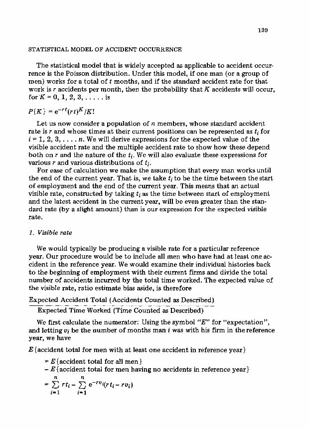
The statistical model that is widely accepted as applicable to accident occur- rence is the Poisson distribution. Under this model, if one man (or a group of men) works for a total of t months, and if the standard accident rate for that work is r accidents per month, then the probability that K accidents will occur, for’K=0,1,2,3 ,..... is

P(K) = e-rt(rt)K/K!

Let us now consider a population of II members, whose standard accident rate is r and whose times at their current positions can be represented as ti for i = 1, 2, 3, . . . . II. We will derive expressions for the expected value of the visible accident rate and the multiple accident rate to show how these depend both on r and the nature of the ti. We will also evaluate these expressions for various r and various distributions of ti.

For ease of calculation we make the assumption that every man works until the end of the current year. That is, we take ti to be the time between the start of employment and the end of the current year. This means that an actual visible rate, constructed by taking ti as the time between start of employment and the latest accident in the current year, will be even greater than the stan- dard rate (by a slight amount) than is our expression for the expected visible rate.

1. Visible rate

We would typically be producing a visible rate for a particular reference year. Our procedure would be to include all men who have had at least one ac- cident in the reference year. We would examine their individual histories back to the beginning of employment with their current firms and divide the total number of accidents incurred by the total time worked. The expected value of the visible rate, ratio estimate bias aside, is therefore

Expected Accident Total (Accidents Counted as Described)

Expected Time Worked (Time Counted as Described)

We first calculate the numerator: Using the symbol “E” for “expectation”, and letting ui be the number of months man i was with his firm in the reference year, we have

E {accident total for men with at least one accident in reference year}

= E {accident total for all men} - E(accident total for men having no accidents in reference year)

= grt i=l

i - ie emrvi(r ti - rui)

140

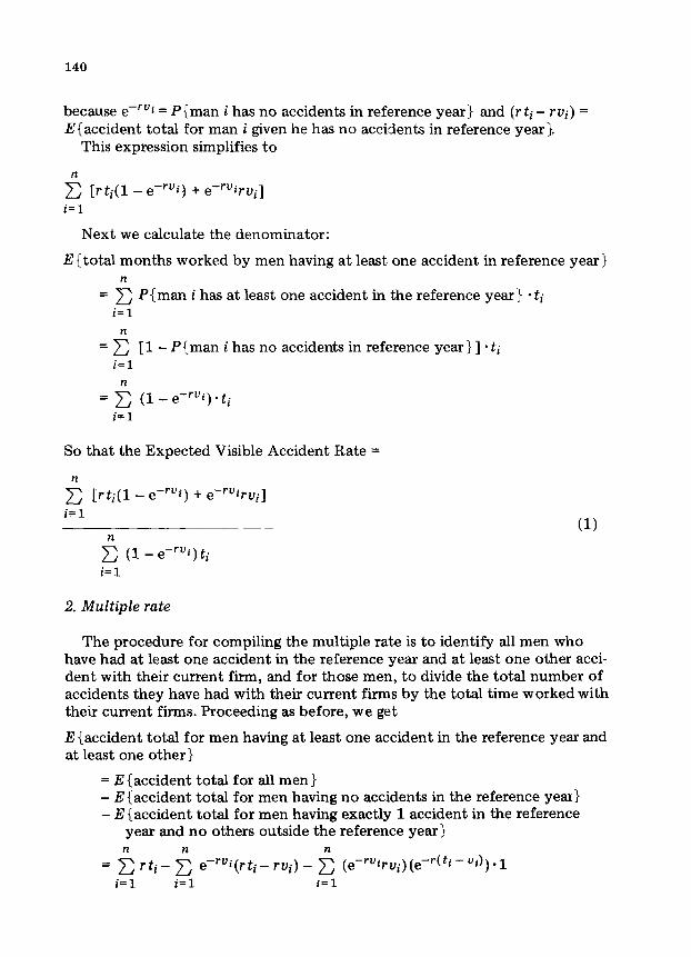
because e-‘“’ I= P{ man i has no accidents in reference year} and (r ti - rui) = E(accident total for man i given he has no accidents in reference year}.

This expression simplifies to

n

C [rti(l - em’“‘) + eTruirui]

i=l

Next we calculate the denominator:

E {total months worked by men having at least one accident in reference year} n

= C P(man i has at least one accident in the reference year} .ti i=l

= 5 [ 1 - P{man i has no accidents in reference year } ] * ti i=l

= 5 (1 _ ewrui) .ti

i=l

So that the Expected Visible Accident Rate =

2 [rti(l - eer”i) + e-‘“irui] i=l

i; (1 - eer”i)ti i=l

2. Multiple rate

The procedure for compiling the multiple rate is to identify all men who have had at least one accident in the reference year and at least one other acci- dent with their current firm, and for those men, to divide the total number of accidents they have had with their current firms by the total time worked with their current firms. Proceeding as before, we get

E {accident total for men having at least one accident in the reference year and at least one other}

= E {accident total for all men} - E {accident total for men having no accidents in the reference year] - E {accident total for men having exactly 1 accident in the reference

year and no others outside the reference year)

= 5 rti- g e-r”i(rti- ‘vi) _ 6 (e-rUirui)(e-r(ti-ui)).l

i=l i=l i=l

141

because

P{man i has exactly 1 accident in reference year and no others outside the reference year}

= P{man i has exactly 1 accident in reference year} *P{man i has none outside the reference year} (by the assum$( pd;p)endence of accident occurrence) = (e-‘“irvi) .e I z

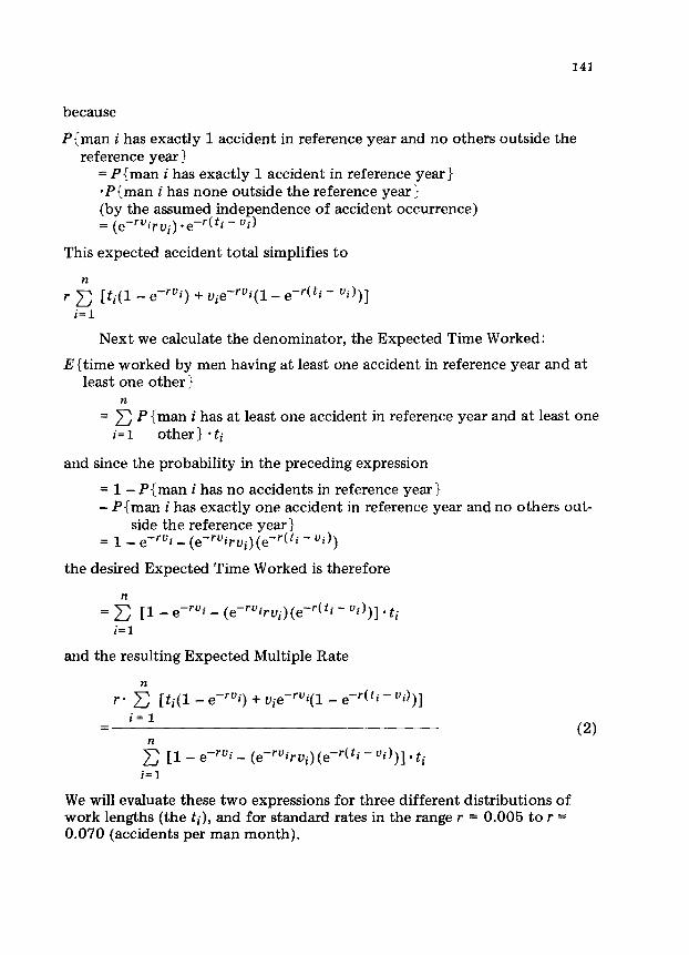
This expected accident total simplifies to

n

a i=l

[ti(l _ e-rui) + vie-rui(l _ e-dti- “i))]

Next we calculate the denominator, the Expected Time Worked:

E { time worked by men having at least one accident in reference year and at least one other}

n = C P {man i has at least one accident in reference year and at least one

i= 1 other } * ti

and since the probability in the preceding expression

= 1 - P{man i has no accidents in reference year} - P{man i has exactly one accident in reference year and no others out-

side the reference year} = 1 - evrui - (e-ruirvi)(e-r(ti - “iI)

the desired Expected Time Worked is therefore

= 5 [l _ emrui _ (evr”irvi)(emr(fi - “i))] . ti

i=l

and the resulting Expected Multiple Rate

n rs C [ti(l _ ewrui) + uieerui(l - e-r(ti-Ui))]

i=l = (2)

i=l

We will evaluate these two expressions for three different distributions of work lengths (the ti), and for standard rates in the range r = 0.005 to r = 0.070 (accidents per man month).

142

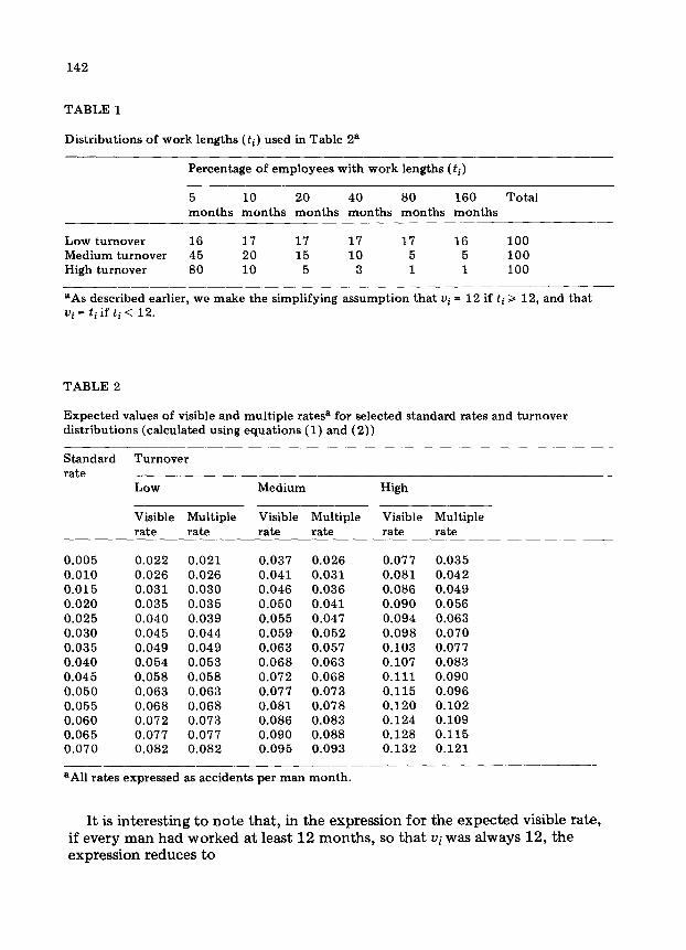
TABLE 1

Distributions of work lengths (ti) used in Table 2*

Percentage of employees with work lengths (ri)

5 10 20 40 80 160 Total months months months months months months

Low turnover 16 17 17 17 17 16 100 Medium turnover 45 20 15 10 5 5 100 High turnover 80 10 5 3 1 1 100

aAs described earlier, we make the simplifying assumption that Ui = 12 if ti > 12, and that Ui = ti if ti < 12.

TABLE 2

Expected values of visible and multiple ratesa for selected standard rates and turnover distributions (calculated using equations (1) and (2))

Standard Turnover rate

Low Medium High

Visible Multiple Visible Multiple Visible Multiple rate rate rate rate rate rate -

0.005 0.022 0.021 0.037 0.026 0.077 0.035 0.010 0.026 0.026 0.041 0.031 0.081 0.042 0.015 0.031 0.030 0.046 0.036 0.086 0.049 0.020 0.035 0.035 0.050 0.041 0.090 0.056 0.025 0.040 0.039 0.055 0.047 0.094 0.063 0.030 0.045 0.044 0.059 0.052 0.098 0.070 0.035 0.049 0.049 0.063 0.057 0.103 0.077 0.040 0.054 0.053 0.068 0.063 0.107 0.083 0.045 0.058 0.058 0.072 0.068 0.111 0.090 0.050 0.063 0.063 0.077 0.073 0.115 0.096 0.055 0.068 0.068 0.081 0.078 0.120 0.102 0.060 0.072 0.073 0.086 0.083 0.124 0.109 0.065 0.077 0.077 0.090 0.088 0.128 0.115 0.070 0.082 0.082 0.095 0.093 0.132 0.121

aAll rates expressed as accidents per man month.

It is interesting to note that, in the expression for the expected visible rate, if every man had worked at least 12 months, so that Ui was always 12, the expression reduces to

143

[

n

r(1 - e-lZr)- c ti + [12nre-lZr] i=l 1 12re’12’

=r+

(1 - e-lZr) - 6 ti

1 _ e-12r ’ -nL a r + +-(3)

C G i=l i=l

gl G

This approximation would be exact if there were zero probability of two or more accidents occurring to the same man in a year:

12re-12’ = PI1 accident in a year} 1 - e-12r = 1 - P{O accidents in a year}

= P{l accident in a year given there cannot be two or more}

Since rz/c .ti is the reciprocal of the average work length, in other words, the i=l

average turnover rate (how frequently the average man changes employment), the expected visible rate is approximately the sum of the average turnover rate and the standard rate, (the validity of the approximation depending on the proportion of men having worked the complete reference year)*.

Furthermore, since the average turnover rate would be estimable from the sample of work lengths for the accident victims, it may be possible to directly subtract the turnover rate from the visible rate to get an estimate of the stan- dard rate. The feasibility of this procedure would depend, of course, on the ac- curacy of the approximating expression for the visible rate.

It is interesting in itself that the average turnover rate would be estimable (in an unbiased sense) from a sample. This is the case because, the effect of experience aside, the probability of an accident occurring to an individual in a given month is independent of his length of time at the job. (Intuition might have suggested that the work lengths would be biased on the high side - more of the accidents occurring to the men with the greater lengths of time.)

We calculate the average turnover rate for the three distributions of work lengths in Table 1:

Distribution Average length Average turnover rate

1 52 months 0.019 2 23 months 0.043 3 10 months 0.100

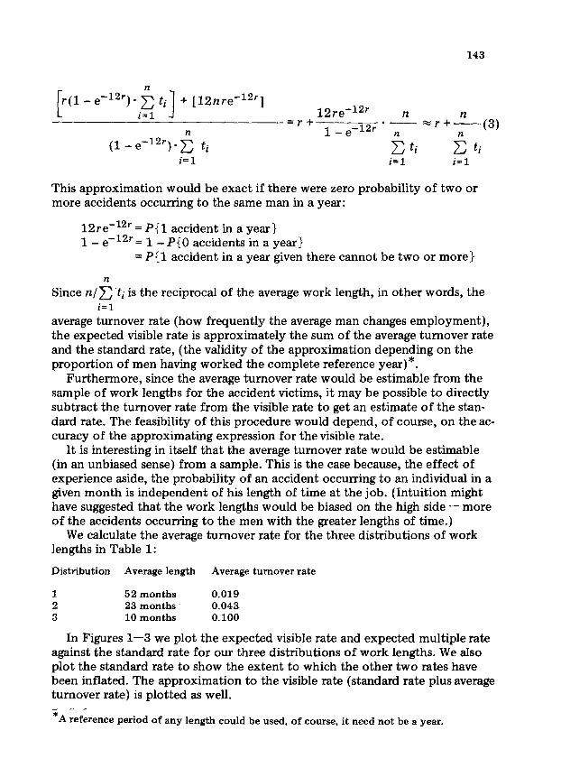
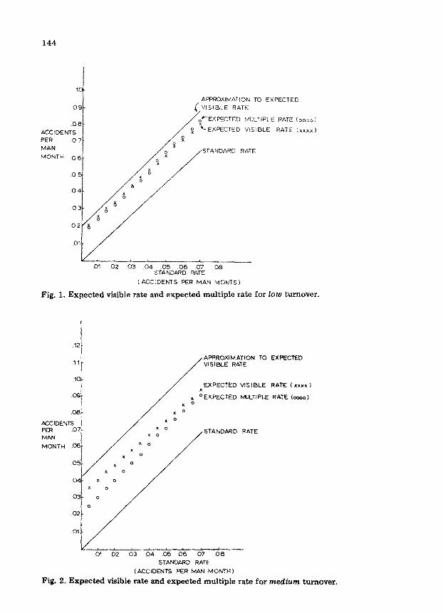
In Figures l-3 we plot the expected visible rate and expected multiple rate against the standard rate for our three distributions of work lengths. We also plot the standard rate to show the extent to which the other two rates have been inflated. The approximation to the visible rate (standard rate plus average turnover rate) is plotted as well.

*A reference period of any length could be used, of course, it need not be a year.

APPROXIMATION TO EXPECTEC

VISIBLE RATE

&Z’.XFECTED MULTIPLE

k EXPECTED VISIBLE

STANDARD RATE

01 02 03 .04 05 06 07 08 STANDARD PATE

(ACCIDENTS PER MAN MONTS)

RATE

RATE

(0400:

(xxxxi

Fig. 1. Expected visible rate and expected multiple rate for low turnover.

AFJPROXIMATION TO EXPECTED VISIBLE RATE

EXPECTED ViSl0LE RATE (xxxx)

0EXPECTED W.JLTIPcE RATE (0000)

STANDARD RATE

M 02 -03 04 05 Q6 07 06

STANDARD RATE

(ACCIDENTS PER MAN MONTH)

Fig. 2. Expected visible rate and expected multiple rate for medium turnover.

145

EXPECTED

RATE ( xxxx )

.E RATE (0000 )

AOJDENTS

PER t

x x 0

x

.08 x 0

MAN Ix o MONTH 07. 0 STANDARD RATE

06. 0

05.

01 02 03 04 05 06 07 06 STANDARD RATE

(ACCIDENTS PER MAN MONTH)

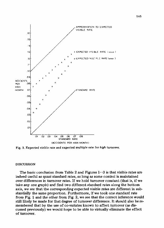
Fig. 3. Expected visible rate and expected multiple rate for high turnover.

DISCUSSION

The basic conclusion from Table 2 and Figures l-3 is that visible rates are indeed useful as quasi standard rates, as long as some control is maintained over differences in turnover rates. If we hold turnover constant (that is, if we take any one graph) and find two different standard rates along the bottom axis, we see that the corresponding expected visible rates are different in sub- stantially the same proportion. Furthermore, if we took one standard rate from Fig. 1 and the other from Fig. 2, we see that the correct inference would still likely be made for that degree of turnover difference. It should also be re- membered that by the use of co-variates known to affect turnover (as dis- cussed previously) we would hope to be able to virtually eliminate the effect of turnover.

146

The multiple rate would appear to be of some additional value, particularly in the area of relatively high turnover. In that instance (Fig. 3) it seems that the multiple rate more closely approximates the standard rate and provides a sharper discrimination than does the visible rate. That is, for real differences in standard rates (unobservable) there would seem to be a greater chance of an ob- servable difference in the multiple rates than in the visible rates. The multiple rate, however, has the accompanying disadvantage of a reduction in sample size. Depending on the specific reduction there may or may not be a net ad- vantage in the use of multiple rates.

EXAMPLE

For an example we turn to our results from The Effect of Piecework on Logging Accident Rates (Mason, 1973). In that study we classified fallers in the logging industry who had an accident in 1972 by: their method of pay- ment (piecework or salary), age, size of firm and location of work. We com- plated each man’s visible rate and used multiple linear regression to see which of the four classifier variables were related to the visible rates. The analysis was then repeated using multiple rates in place of visible rates.

Our findings were that the payment variable was not related to the visible rate but that the other three were. The same basic results were obtained when the multiple rate was used. Actually, although the same variables were found to be significant when multiple rates were used, the firm size variable was then found to be of lesser importance. Perhaps, as previously hypothesized, a com- ponent of the firm-size effect observed in the visible analysis was due to turn- over, so that when the turnover effect was directly minimized by the use of multiple rates that component disappeared. The fact that significance was found for the same variables in the visible rate analysis as in the multiple rate analysis, which was a more direct adjustment for turnover, suggests that the procedure using the visible rate, in which the attempt is to have variation due to turnover removed and accounted for as variation due to (in this case) firm size, may be a satisfactory one. This would be desirable since the sample size reduction with multiple rates would not be incurred. In this example the sample decreased from 1,246 to 211, a reduction that still left us with a useful number but conceivably might not have.

In this particular study, for the group of fallers as a whole, we found that the visible rate was 0.125 and the multiple rate was 0.091. Now, although we don’t know that our turnover model is accurate enough for such a purpose, it is nonetheless interesting to note that from the magnitude of the rates and from the observation that the multiple rate is less than the visible rate, lve can see that this particular situation is approximately described by Fig. 3; and furthermore, that the visible rate of 0.125 and multiple rate of 0.091 suggest that the true standard rate would be in the range 0.040 to 0.060.

147

ACKNOWLEDGMENTS

Many thanks are due Mrs. Sandi Bellamy and Mrs. Carol Christopher for their careful typing of the drafts of this paper.

REFERENCES

Cresswell, W.L. and Frogatt, P., 1963. The Causation of Bus Driver Accidents. Oxford University Press, London.

Gordejko, O.N. and Kirpicenko, V.E., 1973. Investigation into the Statistical Distribution of Accidents. Naucynye Raboty Institutov Ohrany Truda VCSPS, Moscow.

Mason, K., 1973. The effect of piecework on logging accident rates (Incorporating a differ ent approach to the exposure problem). Workmen’s Compensation Board of British Columbia, Vancouver B.C. (Listed in the Catalogue of Educational Resources of the Canada Safety Council).

Mintz, A., 1954. The inference of accident liability from the accident record. Journal of Applied Psychology, 38: 41-46.