Violations of the Constant Variances Assumption - … Notes/Variances.pdf · Violations of the Constant Variances ... Suppose we generate some arti cial data in which the residual

Violations of the Constant Variances Assumption

James H. Steiger

Department of Psychology and Human DevelopmentVanderbilt University

James H. Steiger (Vanderbilt University) Violations of the Constant Variances Assumption 1 / 19

Violations of the Constant Variances Assumption1

A Diagnostic for Nonconstant Variance


Introduction

The assumption of constant conditional variance is a staple of the standard linearregression model, both in the case of a single predictor-regressor (bivariate regression) orin the case of several predictors (multiple regression).Violation of this assumption occurs quite frequently in practice, for a number of reasons.In this module, we’ll explore a diagnostic significance test sometimes used to assessdepartures from the equal variances assumption.




Breusch and Pagan (1979) gave a test for nonconstant variance. This was also developedindependently by Cook and Weisberg(1983) and discussed in section 7.2.2 of the ALR4text.The test assumes that the conditional variance of Y given X is an exponential function ofan unknown parameter vector and some set of regressors Z . The assumption is that

Var(Y |X ,Z = z) = σ2 exp(λ′z) (1)

If λ = 0, then the right side of the equation evaluates to σ2, and we have constantvariance.Under that assumption, a score test that λ = 0 can be computed using regressionsoftware.




Compute the standard OLS fit. Save the residuals ei .Compute scaled residuals ui = e2i /σ

2. The maximum likelihood estimator σ2 is simply∑e2i /n, i.e., it uses n instead of n − p − 1 as a denominator. The variable U is simply

composed of the ui .Compute the regression for the mean function E (U|Z = z) = λ0 + λ′z. Obtain SSreg forthis regression with degrees of freedom equal to q, the number of components in Z . Ifvariance is thought to be a function of the responses (i.e., the dependent variable Y ),then in this regression replace Z by the fitted values of the regression in step 1, in whichcase the test will have 1 degree of freedom.The score test statistic is S = SSreg/2. The reference distribution is χ2

q.




If you have more than one predictor, you can perform the B-P test on differentcombinations of regressors based on those predictors, in order to develop a model for thevariance function.Let’s start with a simple bivariate regression.Suppose we generate some artificial data in which the residual variance is a function of X .

> set.seed(12345)

> x <- 1:100

> y <- 2*x + 5 + x * rnorm(100)

> plot(x,y)

0 20 40 60 80 100

010

020

030

040

0

x

y



A Diagnostic for Nonconstant VarianceHere are the manual calculations:

> m0 <- lm(y ~ x)

> sig2 <- sum(residuals(m0)^2)/length(x)

> U <- residuals(m0)^2/sig2

> m1 <- lm(U~x)

> anova(m1)

Analysis of Variance Table

Response: U

Df Sum Sq Mean Sq F value Pr(>F)

x 1 65.233 65.233 34.272 6.383e-08 ***

Residuals 98 186.533 1.903

---

Signif. codes: 0 '***' 0.001 '**' 0.01 '*' 0.05 '.' 0.1 ' ' 1

> S <- anova(m1)$'Sum Sq'[1]/2> p.value <- 1-pchisq(S,1)

> S

[1] 32.61656

> p.value

[1] 1.122545e-08



A Diagnostic for Nonconstant VarianceThe Snow Geese Data

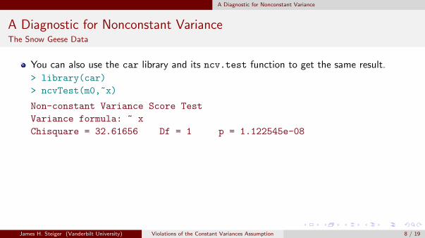
You can also use the car library and its ncv.test function to get the same result.

> library(car)

> ncvTest(m0,~x)

Non-constant Variance Score Test

Variance formula: ~ x

Chisquare = 32.61656 Df = 1 p = 1.122545e-08




Aerial surveys sometimes rely on visual methods to estimate the number of animals in anarea. For example, to study snow geese in their summer range areas west of Hudson Bayin Canada, small aircraft were used to fly over the range, and when a flock of geese wasspotted, an experienced person estimated the number of geese in the flock.To investigate the reliability of this method of counting, an experiment was conducted inwhich an airplane carrying two observers flew over n = 45 flocks, and each observer madean independent estimate of the number of birds in each flock.Also, a photograph of the flock was taken so that a more or less exact count of thenumber of birds in the flock could be made.The resulting data are given in the data file snowgeese.txt (Cook and Jacobson, 1978).The three variables in the data set are Photo = photo count, Obs1 = aerial count byobserver one and Obs2 = aerial count by observer 2.




Here we demonstrate calculation of the test statistic. This demonstration uses thesnowgeese data.

> data(snowgeese)

> attach(snowgeese)

> library(xtable)

> m1 <- lm(photo~obs1,snowgeese)

> sig2 <- sum(residuals(m1)^2)/length(snowgeese$obs1)

> U <- residuals(m1)^2/sig2

> m2 <- lm(U~snowgeese$obs1)

> anova(m2)

Analysis of Variance Table

Response: U

Df Sum Sq Mean Sq F value Pr(>F)

snowgeese$obs1 1 162.83 162.826 50.779 8.459e-09 ***

Residuals 43 137.88 3.207

---

Signif. codes: 0 '***' 0.001 '**' 0.01 '*' 0.05 '.' 0.1 ' ' 1

> S <- anova(m2)$'Sum Sq'[1]/2> p.value <- 1-pchisq(S,1)

> S

[1] 81.41318

> p.value

[1] 0




However, a much easier way to do it is to use the library lmtest, then employ thebptest function,To get the same output as ALR, you have to set the option studentize=FALSE.

> library(lmtest)

> bptest(photo~obs1,studentize=F)

Breusch-Pagan test

data: photo ~ obs1

BP = 81.4132, df = 1, p-value < 2.2e-16

You can also use the car library and its ncv.test function

> library(car)

> ncvTest(m1,~obs1)

Non-constant Variance Score Test

Variance formula: ~ obs1

Chisquare = 81.41318 Df = 1 p = 1.831324e-19



A Diagnostic for Nonconstant VarianceThe Sniffer Data

The sniffer data example on page 166–167 of ALR4 implement the Breusch-Paganstatistic in diagnosing and compensating for nonconstant variance.When gasoline is pumped into a tank, hydrocarbon vapors are forced out of the tank andinto the atmosphere.To reduce this significant source of air pollution, devices are installed to capture the vapor.In testing these vapor recovery systems, a “sniffer” measures the amount recovered.To estimate the efficiency of the system, some method of estimating the total amountgiven off must be used.




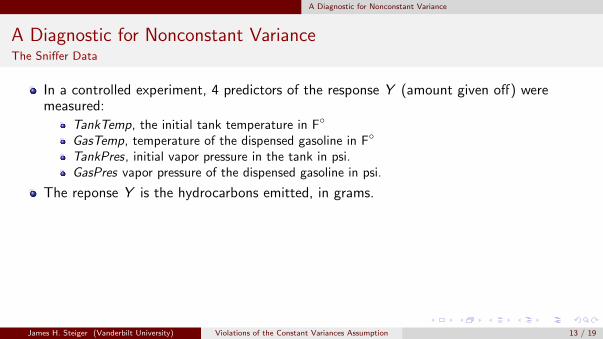
In a controlled experiment, 4 predictors of the response Y (amount given off) weremeasured:

TankTemp, the initial tank temperature in F◦

GasTemp, temperature of the dispensed gasoline in F◦

TankPres, initial vapor pressure in the tank in psi.GasPres vapor pressure of the dispensed gasoline in psi.

The reponse Y is the hydrocarbons emitted, in grams.




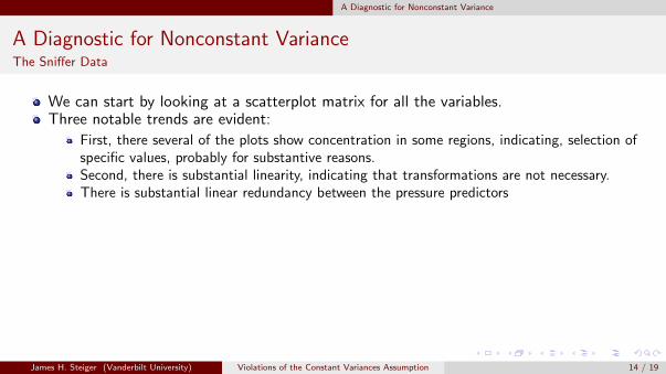
We can start by looking at a scatterplot matrix for all the variables.Three notable trends are evident:

First, there several of the plots show concentration in some regions, indicating, selection ofspecific values, probably for substantive reasons.Second, there is substantial linearity, indicating that transformations are not necessary.There is substantial linear redundancy between the pressure predictors




> data(sniffer)

> attach(sniffer)

> pairs(sniffer)

TankTemp

40 60 80 3 4 5 6 7

3050

7090

4060

80

GasTemp

TankPres

34

56

7

34

56

7

GasPres

30 50 70 90 3 4 5 6 7 20 30 40 50

2040Y




Examining some residual plots using the code below, we see that variance does seem toincrease from left to right in plots of TankTemp and GasPres.

> pdf("ALR_FIG0810.pdf", onefile=T)

> m1 <- lm(Y~TankTemp+GasTemp+TankPres+GasPres,sniffer)

> op<-par(mfrow=c(2,2),mar=c(4,3,0,.5)+.1,mgp=c(2,1,0))

> plot(predict(m1),residuals(m1),xlab="(a) Yhat", ylab="Residuals")

> abline(h=0)

> plot(TankTemp,residuals(m1),xlab="(b) Tank temperature",

+ ylab="Residuals")

> abline(h=0)

> plot(GasPres,residuals(m1),xlab="(c) Gas pressure",

+ ylab="Residuals")

> abline(h=0)

> U <- residuals(m1)^2*125/(sum(residuals(m1)^2))

> m3 <- update(m1,U~.)

> plot(predict(m3),residuals(m1),xlab="(d) Linear combination",

+ ylab="Residuals")

> abline(h=0)




20 25 30 35 40 45 50

−6

−4

−2

02

46

(a) Yhat

Res

idua

ls

30 40 50 60 70 80 90

−6

−4

−2

02

46

(b) Tank temperature

Res

idua

ls

3 4 5 6 7

−6

−4

−2

02

46

(c) Gas pressure

Res

idua

ls

−0.5 0.0 0.5 1.0 1.5 2.0

−6

−4

−2

02

46

(d) Linear combination

Res

idua

ls




Weisberg goes on to conduct a sequence of tests for nonconstant variance under choice ofvarious predictors. Results are displayed in Table 7.4, page 167:

By subtraction, we can compare nested models, with a χ2 difference test. The differencebetween two nested model χ2 statistics, χ2

a − χ2b, has an approximate χ2 distribution with

dfa − dfb degrees of freedom.In this case, if we first compare the statistic for TankTemp, GasPres with the statisticfor TankTemp, we find that the difference test has a χ2 = 11.78− 9.71 = 2.07 with 1degree of freedom, which is not significant, indicating that GasPres does not improve theprediction of variance significantly better than TankTemp.We also see that adding three additional predictors does not improve significantly over theuse of TankTemp, as the difference statistic is χ2

3 = 13.76− 9.71 = 4.05, which is alsononsignificant.




We arrive at the decision to model the variance as

Var(Y |X ,Z ) = σ2 × TankTemp (2)

thereby using 1/TankTemp values as weights in weighted least squares.Note. If you compare the above with the discussion on page 166 of ALR4, you willdiscover that the textbook has an error. This traces back to ALR3, the previous edition.In ALR3, the corresponding table (Table 8.4 in ALR3) had the test statistics forTankTemp and GasPres reversed.The discussion in ALR3 was based on those reversed values.The table was corrected in ALR4, but unfortunately the discussion was not.


Documents

Violations of the Constant Variances Assumption - … Notes/Variances.pdf · Violations of the Constant Variances ... Suppose we generate some arti cial data in which the residual