Extended nonlocal games

by

Vincent Russo

A thesispresented to the University of Waterloo

in fulfillment of thethesis requirement for the degree of

Doctor of Philosophyin

Computer Science

Waterloo, Ontario, Canada, 2017c© Vincent Russo 2017ar

Xiv

:170

4.07

375v

1 [

quan

t-ph

] 2

4 A

pr 2

017

Examining Committee Membership

The following served on the Examining Committee for this thesis. The decision of theExamining Committee is by majority vote.

External Examiner STEPHANIE WEHNERProfessor

Supervisors JOHN WATROUSProfessorMICHELE MOSCAProfessor

Internal Members RICHARD CLEVEProfessorDEBBIE LEUNGProfessor

Internal-external Member VERN PAULSENProfessor

Defence Chair SUE HORTONProfessor

ii

I hereby declare that I am the sole author of this thesis. This is a true copy of the thesis,including any required final revisions, as accepted by my examiners.

I understand that my thesis may be made electronically available to the public.

iii

Abstract

The notions of entanglement and nonlocality are among the most striking ingredientsfound in quantum information theory. One tool to better understand these notions is themodel of nonlocal games ; a mathematical framework that abstractly models a physicalsystem. The simplest instance of a nonlocal game involves two players, Alice and Bob,who are not allowed to communicate with each other once the game has started and whoplay cooperatively against an adversary referred to as the referee.

The focus of this thesis is a class of games called extended nonlocal games, of whichnonlocal games are a subset. In an extended nonlocal game, the players initially share atripartite state with the referee. In such games, the winning conditions for Alice and Bobmay depend on outcomes of measurements made by the referee, on its part of the sharedquantum state, in addition to Alice and Bob’s answers to the questions sent by the referee.

We build up the framework for extended nonlocal games and study their properties andhow they relate to nonlocal games. In doing so, we study the types of strategies that Aliceand Bob may adopt in such a game. For instance, we refer to strategies where Alice andBob use quantum resources as standard quantum strategies and strategies where there is anabsence of entanglement as an unentangled strategy. These formulations of strategies arepurposefully reminiscent of the respective quantum and classical strategies that Alice andBob use in a nonlocal game, and we also consider other types of strategies with a similarcorrespondence for the class of extended nonlocal games.

We consider the value of an extended nonlocal game when Alice and Bob apply aparticular strategy, again in a similar manner to the class of nonlocal games. Unlikecomputing the unentangled value where tractable algorithms exist, directly computing thestandard quantum value of an extended nonlocal game is an intractable problem. Weintroduce a technique that allows one to place upper bounds on the standard quantumvalue of an extended nonlocal game. Our technique is a generalization of what we refer toas the QC hierarchy which was studied independently in works by Doherty, Liang, Toner,and Wehner as well as by Navascues, Pironio, and Acın. This technique yields an upperbound approximation for the quantum value of a nonlocal game.

We also consider the question of whether or not the dimensionality of the state thatAlice and Bob share as part of their standard quantum strategy makes any difference inhow well they can play the game. That is, does there exist an extended nonlocal gamewhere Alice and Bob can win with a higher probability if they share a state where thedimension is infinite? We answer this question in the affirmative and provide a specificexample of an extended nonlocal game that exhibits this behavior.

iv

We study a type of extended nonlocal game referred to as a monogamy-of-entanglementgame, introduced by Tomamichel, Fehr, Kaniewski, and Wehner, and present a numberof new results for this class of game. Specifically, we consider how the standard quantumvalue and unentangled value of these games relate to each other. We find that for certainclasses of monogamy-of-entanglement games, Alice and Bob stand to gain no benefit inusing a standard quantum strategy over an unentangled strategy, that is, they performjust as well without making use of entanglement in their strategy. However, we show thatthere does exist a monogamy-of-entanglement game in which Alice and Bob do performstrictly better if they make use of a standard quantum strategy. We also analyze theparallel repetition of monogamy-of-entanglement games; the study of how a game performswhen there are multiple instances of the game played independently. We find that certainclasses of monogamy-of-entanglement games obey strong parallel repetition. In contrast,when Alice and Bob use a non-signaling strategy in a monogamy-of-entanglement game,we find that strong parallel repetition is not obeyed.

v

Acknowledgements

I am greatly indebted to my advisors John Watrous and Michele Mosca for their guid-ance throughout the course of my studies. John is an incredible supervisor and one that Ihave been exceptionally lucky to have had the pleasure of working with. John’s attentionto detail and sense of humour has greatly impacted my own approach to science and lifein general. I am truly humbled by John’s command of mathematical rigour and writingclarity. I am also incredibly grateful to Mike, for including me in the quantum circuitsgroup and enabling me to take part in internships.

Gratitude is also due to professors Richard Cleve, Debbie Leung, Vern Paulsen, andStephanie Wehner for taking their valuable time to serve on my defence committee. Ithank them greatly for their input.

Throughout my studies, I’ve been lucky enough to work with some outstanding stu-dents, post-doctoral researchers, and professors. Many thanks are due to Nathaniel John-ston, Rajat Mittal, Matthew Pusey, Jamie Sikora, William Slofstra, Thomas Vidick, andothers who were always willing to discuss interesting ideas and explain abstract conceptsto me.

My time at IQC and in Waterloo has been full of great people and experiences. I wishto thank Sascha Agne, Srinivasan Arunachalam, Alessandro Cosentino, Arnaud Carignan-Dugas, Maria Kieferova, Robin Kothari, Anirudh Krishna, Vinayak Pathak, Dan Puzzuoli,Yuval Sanders, Basil Singer, Marco Shum, Zak Webb, and the students and faculty of IQCfor making my time here incredibly enjoyable. I sincerely hope that we keep in touch asour journeys continue. Thanks are also due to the excellent administrative support of IQCand DC for always being able to quickly resolve any technical issues in running softwarefor experiments.

To my “urban planning” circle of friends, thank you for making me an honorary memberof the group, and accepting me even though I’m in computer science! You have beenmy strongest support network and my best friends in Waterloo. I will sorely miss ourmany political conversations and random adventures. To my musically inclined friendsJaden Hellmann, Alexandar Smith, Will Towns, and Cody Veal, our jam sessions andmiscellaneous discussions were a welcome creative distraction from research.

To my friends back home in Michigan, I thank you for understanding my absence.Thanks to Kenny G., Sara Gilhooly, Alex, Nick, and Rachel Marowsky, Mike Sanderson,Ryan Seiler, Joe Sousa, Ryan Trainor, and Matt Wolford. Whenever I’ve been back tovisit, I was always warmly received.

vi

I also extend gratitude toward the hospitality received during my internships. I thankBBN Raytheon, specifically Richard Lazarus, Andrei Lapets, and Marcus da Silva forallowing me to contribute to many interesting projects.

I cannot express enough gratitude toward my family for their encouragement, love, andsupport. My brothers Joey and Matthew, and my sister Theresa and her husband Colin.I also thank Beth Russo and Lauren Kisic, my Aunt Cathy, Uncle Dan, Uncle John, UncleSteve, and Aunt Marie for a lifetime of support. A sincere and heartfelt thanks are dueto my parents James and Marjorie Russo, who have always nurtured and encouraged myinterests, whatever they may have been, and for their seemingly endless wells of love andsupport.

Lastly, I thank Paulina Rodriguez. Your support, love, and encouragement throughoutthis journey cannot be overstated. This document is as much a part of me as it is a partof you. I love you.

For all of those who I did not mention by name, please accept my sincerest apologies,and know that this document is a testament to your encouragement and support. Thankyou all.

vii

Dedication

This thesis is dedicated to those who have shaped my life, but no longer walk with methrough it. My grandparents Anthony and Jean Russo, Ben Benton, my Aunt Alice, andmy second moms, Denise Marowsky and Debbie Gilhooly.

viii

Table of Contents

List of Tables xiii

List of Figures xiv

1 Introduction 1

1.1 Summary of the results . . . . . . . . . . . . . . . . . . . . . . . . . . . . . 2

1.2 Overview . . . . . . . . . . . . . . . . . . . . . . . . . . . . . . . . . . . . . 3

2 Preliminaries 6

2.1 Basic notation, terminology, and background . . . . . . . . . . . . . . . . . 7

2.1.1 Alphabets, symbols, and strings . . . . . . . . . . . . . . . . . . . . 7

2.1.2 Vectors, operators, and mappings . . . . . . . . . . . . . . . . . . . 7

2.1.3 Operator decompositions and vector decompositions . . . . . . . . . 14

2.1.4 Convexity and semidefinite programming . . . . . . . . . . . . . . . 15

2.2 Quantum information theory . . . . . . . . . . . . . . . . . . . . . . . . . . 18

2.2.1 Quantum states, operations, and measurements . . . . . . . . . . . 18

2.2.2 Entanglement and separability . . . . . . . . . . . . . . . . . . . . . 20

2.2.3 Teleportation . . . . . . . . . . . . . . . . . . . . . . . . . . . . . . 23

2.3 The nonlocal game model . . . . . . . . . . . . . . . . . . . . . . . . . . . 24

2.3.1 Strategies for nonlocal games . . . . . . . . . . . . . . . . . . . . . 26

2.3.2 Relationships between different strategies and values . . . . . . . . 31

ix

3 Extended Nonlocal Games 34

3.1 The extended nonlocal game model . . . . . . . . . . . . . . . . . . . . . . 35

3.2 Strategies for extended nonlocal games . . . . . . . . . . . . . . . . . . . . 36

3.2.1 Extended nonlocal games and assemblage operators . . . . . . . . . 36

3.2.2 Standard quantum strategies for extended nonlocal games . . . . . 37

3.2.3 Unentangled strategies for extended nonlocal games . . . . . . . . . 40

3.2.4 Commuting measurement strategies for extended nonlocal games . . 41

3.2.5 Non-signaling strategies for extended nonlocal games . . . . . . . . 42

4 On the properties of the extended nonlocal game model 44

4.1 Quantum-classical games . . . . . . . . . . . . . . . . . . . . . . . . . . . . 45

4.2 Constructing extended nonlocal games from quantum-classical games . . . 48

4.2.1 Teleportation games and quantum-classical games . . . . . . . . . . 49

4.2.2 Extended nonlocal games and teleportation games . . . . . . . . . . 55

4.3 Variations on the extended nonlocal game model . . . . . . . . . . . . . . . 62

4.3.1 Quantum-classical-quantum extended nonlocal games . . . . . . . . 63

5 Bounding the standard quantum value of extended nonlocal games 66

5.1 Upper bounds for extended nonlocal games: the extended QC hierarchy . . 67

5.1.1 Intuitive description of the extended QC hierarchy . . . . . . . . . . 67

5.1.2 Construction of the extended QC hierarchy . . . . . . . . . . . . . . 73

5.1.3 Convergence of the extended QC hierarchy . . . . . . . . . . . . . . 75

5.1.4 Examples: Upper-bounding the standard quantum values of extendednonlocal games . . . . . . . . . . . . . . . . . . . . . . . . . . . . . 81

5.2 Lower bounds for extended nonlocal games: the see-saw method . . . . . . 85

5.2.1 Examples: Lower-bounding the standard quantum values of extendednonlocal games . . . . . . . . . . . . . . . . . . . . . . . . . . . . . 87

x

6 Monogamy-of-Entanglement Games 89

6.1 Monogamy-of-entanglement games . . . . . . . . . . . . . . . . . . . . . . . 90

6.1.1 Strategies and values of monogamy-of-entanglement games . . . . . 91

6.1.2 The BB84 monogamy-of-entanglement game . . . . . . . . . . . . . 93

6.1.3 Comparing standard quantum and unentangled strategies for monogamy-of-entanglement games . . . . . . . . . . . . . . . . . . . . . . . . . 94

6.2 Parallel repetition of monogamy-of-entanglement games . . . . . . . . . . . 96

6.2.1 Strong parallel repetition for certain monogamy-of-entanglement gameswith two questions . . . . . . . . . . . . . . . . . . . . . . . . . . . 100

6.2.2 No strong parallel repetition for monogamy-of-entanglement gameswith non-signaling provers . . . . . . . . . . . . . . . . . . . . . . . 102

6.3 Upper and lower bounds on monogamy-of-entanglement games . . . . . . . 103

6.3.1 A monogamy-of-entanglement game with quantum advantage . . . 103

6.3.2 Synopsis of monogamy-of-entanglement games . . . . . . . . . . . . 104

7 Conclusions and open problems 106

References 110

APPENDICES 117

A Software 118

A.1 Software Listings . . . . . . . . . . . . . . . . . . . . . . . . . . . . . . . . 119

A.1.1 The first level of the extended QC hierarchy for the BB84 extendednonlocal game . . . . . . . . . . . . . . . . . . . . . . . . . . . . . . 119

A.1.2 The first level of the extended QC hierarchy for the CHSH extendednonlocal game . . . . . . . . . . . . . . . . . . . . . . . . . . . . . . 121

A.1.3 The non-signaling value for the CHSH extended nonlocal game . . . 125

A.1.4 Implementation of the see-saw method for computing lower boundson the BB84 extended nonlocal game . . . . . . . . . . . . . . . . . 127

A.1.5 The BB84 monogamy game (Example 6.1) . . . . . . . . . . . . . . 131

xi

A.1.6 A monogamy-of-entanglement game defined by mutually unbiasedbases (Example 6.8) . . . . . . . . . . . . . . . . . . . . . . . . . . 132

A.1.7 A counter-example to strong parallel repetition for monogamy-of-entanglement games with non-signaling provers (Proof of Theorem6.7) . . . . . . . . . . . . . . . . . . . . . . . . . . . . . . . . . . . . 133

xii

List of Tables

6.1 Results on monogamy-of-entanglement games. . . . . . . . . . . . . . . . . 105

xiii

List of Figures

2.1 The teleportation protocol. . . . . . . . . . . . . . . . . . . . . . . . . . . . 23

2.2 A two-player nonlocal game. . . . . . . . . . . . . . . . . . . . . . . . . . . 28

3.1 A two-player extended nonlocal game. . . . . . . . . . . . . . . . . . . . . 38

4.1 A quantum strategy for a quantum-classical game. . . . . . . . . . . . . . . 46

4.2 A quantum strategy for a teleportation game. . . . . . . . . . . . . . . . . 51

4.3 A teleportation game strategy. . . . . . . . . . . . . . . . . . . . . . . . . . 54

4.4 The extended nonlocal game Ht. . . . . . . . . . . . . . . . . . . . . . . . . 59

4.5 A quantum-classical-quantum extended nonlocal game. . . . . . . . . . . . 65

5.1 Levels of the extended QC hierarchy. . . . . . . . . . . . . . . . . . . . . . 72

6.1 A monogamy-of-entanglement game. . . . . . . . . . . . . . . . . . . . . . 91

6.2 Parallel repetition of a monogamy-of-entanglement game. . . . . . . . . . . 98

xiv

Chapter 1

Introduction

The model of two player games has served an important role in developing our under-standing of theoretical computer science and quantum information. In such a game, weconsider the players, referred to as Alice and Bob, who are not allowed to communicateto each other once the game begins, and who play cooperatively against a party referredto as the referee. The game begins when the referee asks questions to Alice and Bob towhich they must respond. When Alice and Bob send back the responses to the referee, thereferee evaluates the questions and answers against a criterion that is publicly known tothe referee, Alice, and Bob that determines what constitutes a winning or losing outcome.

A primary challenge that arises when studying these games is to determine the maxi-mum probability with which Alice and Bob are able to achieve a winning outcome. Thisprobability is highly dependent on the type of strategy that Alice and Bob use in the game.Before the game begins, Alice and Bob are free to communicate with each other and decideon the type of strategy they will use.

A classical strategy is one in which Alice and Bob decide on a deterministic mapping ofoutputs for every possible combination of inputs they will receive in the game. The corre-sponding maximum probability achieved when Alice and Bob employ a classical strategyis referred to as the classical value of the game.

Another type of strategy called a quantum strategy is one in which Alice and Bob areallowed to use nonlocal resources. This type of strategy may involve Alice and Bob sharingan arbitrary entangled state prior to the start of the game along with sets of measurementsthat they may apply to their portions of the state after they each receive questions fromthe referee. The corresponding maximum probability achieved when Alice and Bob use aquantum strategy is referred to as the quantum value of the game.

1

For certain games, the probability that Alice and Bob obtain a winning outcome ishigher if they use a quantum strategy as opposed to a classical one. This striking separationis one primary motivation to study nonlocal games, as it provides examples of tasks thatbenefit from the manipulation of quantum information. Indeed, the model of nonlocalgames have been widely studied, especially in recent years [CHTW04, BBT05, CSUU08,DLTW08, KR10, KRT10, KKM+11, JP11, BFS13, RV15, DSV13, Vid13, CM14].

The ability to calculate the quantum value for an arbitrary nonlocal game is a highlynon-trivial task. Indeed, the quantum value is only known in special cases for certainnonlocal games. For an arbitrary nonlocal game, there exist approaches that place upperand lower bounds on the quantum value. One such approach (that we refer to as the QChierarchy as done in [CV15] and was introduced in [DLTW08, NPA07]), is implementedas a hierarchy of optimization problems, referred to as semidefinite programs, which areoptimization problems where the constraints are semidefinite. Convergence is guaranteedfrom the QC hierarchy, yet it may be intractable to compute. The lower bound approachis also calculated using the technique of semidefinite programming [LD07]. While thismethod is more efficient to carry out, it does not guarantee convergence to the quantumvalue (although in certain cases, it is attained).

In a nonlocal game, the referee is only responsible for sending questions, receivinganswers, and evaluating whether the selection of questions and respective answers yieldsa winning or losing outcome. In this thesis, we consider a generalization of the nonlocalgame model where the referee is provided with part of a quantum system prepared byAlice and Bob, and in addition, also has sets of measurements that he may apply to hisportion of the quantum system to determine the outcome of the game. This type of gameis referred to as an extended nonlocal game. Extended nonlocal games constitute a widerclass of games of which nonlocal games are a subset. For instance, an extended nonlocalgame where the dimension of the quantum system held by the referee is one-dimensionalis precisely a nonlocal game. Monogamy-of-entanglement games are a special type ofextended nonlocal game introduced in [TFKW13] that has been studied with respect tothe problem of position-based cryptography.

1.1 Summary of the results

In addition to introducing the model of extended nonlocal games, we prove the followingresults:

• We prove that there exists a class of extended nonlocal game for which no finite-

2

dimensional quantum strategy can be optimal. This result further implies the ex-istence of a tripartite steering inequality for which an infinite-dimensional quantumstate is required in order to achieve maximal violation.

• We generalize the QC hierarchy, a technique for providing upper bounds on nonlocalgames, to the case of extended nonlocal games. We also present a method based onthe see-saw algorithm of Liang and Doherty [LD07] that provides lower bounds onthe class of extended nonlocal games.

• We present a number of results about the class of monogamy-of-entanglement games,which are a specific type of extended nonlocal game. Specifically, we show that:

– Monogamy-of-entanglement games obey strong parallel repetition when the sizeof the question set has 2 elements and the size of the answer set is arbitrary,and the sets of measurements used by the referee are projective.

– Monogamy-of-entanglement games do not obey strong parallel repetition whenthe players use non-signaling strategies.

– We present a class of monogamy-of-entanglement games where the size of thequestion set has 2 elements and the size of the answer set is arbitrary whereAlice and Bob can always achieve the quantum value of such a game by usinga strategy that does not require them to store quantum information.

– There exists a monogamy-of-entanglement game in which the size of the questionset has 4 elements and the answer set has 3 elements, for which Alice and Bobmust store quantum information to play optimally.

1.2 Overview

We assume familiarity with the basic notions of quantum computation and quantum in-formation as can be found in [NC00]. It may also be helpful to have a familiarity withthe terminology and mathematics in the first two chapters of [Wat15], although we shallalso attempt a self-contained presentation of the necessary tools needed to understand thecontent herein. Throughout this thesis, we also make frequent use of the mathematicaltool of semidefinite programming. Supplementary resources for the interested reader canbe found in lecture 7 of [Wat04] as well as [BV04].

In Chapter 2, we review the basics of quantum information, nonlocal games, and rele-vant notation that will be used in the remainder of this thesis.

3

In Chapter 3, we introduce the model of extended nonlocal games that is built uponthe model of nonlocal games.

In Chapter 4, we present an analysis of certain properties of the extended nonlocal gamemodel and give an example of an extended nonlocal game for which no finite-dimensionalquantum strategy can be optimal.

In Chapter 5, we present a method that provides upper and lower bounds on the valueof an extended nonlocal game.

In Chapter 6, we study the class of extended nonlocal games referred to as monogamy-of-entanglement games and prove a number of properties that these games exhibit.

Finally, in Chapter 7, we present conclusions and pose open questions that may be ofinterest for future research. Supplementary software used in this thesis is also provided inAppendix A, as well as on the software repositories hosted here [Rus15] and here [Rus16].

The following is a list of existing work directly related to the content in this document:

• V. Russo and J. Watrous. Extended nonlocal games from quantum-classicalgames. 2016, [RW16].

• N. Johnston, R. Mittal, V. Russo, and J. Watrous. Extended nonlocal gamesand monogamy-of-entanglement games. Proc. R. Soc. A 472:20160003, 2016,[JMRW16].

The following is a list of existing work completed during my Ph.D., but not directly relatedto my thesis work:

• S. Bandyopadhyay, A. Cosentino, N. Johnston, V. Russo, J. Watrous, and N. Yu.Limitations on separable measurements by convex optimization. IEEETransactions on Information Theory, 2015, [BCJ+15].

• S. Arunachalam, N. Johnston, and V. Russo. Is absolute separability deter-mined by the partial transpose?. Quantum Information & Computation, 2015,[AJR15].

• D. Gosset, V. Kliuchinikov, M. Mosca, and V. Russo. An algorithm for the T-count. Quantum Information & Computation, 2014, [GKMR14].

• A. Cosentino and V. Russo. Small sets of locally indistinguishable orthogo-nal maximally entangled states. Quantum Information & Computation, 2014,[CR14].

4

• S. Arunachalam, A. Molina, and V. Russo. Quantum hedging in two-roundprover-verifier interactions. arXiv:1310.7954, 2013, [AMR13].

5

Chapter 2

Preliminaries

In this chapter, we present an overview of the relevant subject matter of quantum infor-mation theory that will be used for the remainder of this thesis. We further establish basicterminology and notation. We shall make gratuitous use of the notation conventions forquantum information theory from [Wat15]. The reader is assumed to be familiar with thebasic underpinnings of quantum information theory, as may be found, for instance, in thefollowing references [NC00, KLM07, Wil13].

We also introduce the subject of convex optimization, which as we shall see, acts as aSwiss army knife for many problems of interest in quantum information, and indeed manythat we will encounter in this thesis. For further information on convex optimization, thereader is referred to [BV04].

We shall then introduce the nonlocal game formalism. This model provides an excel-lent venue to abstractly study one of the most crucial features of quantum information:entanglement. We shall formally define the nonlocal game model and present relevantbackground work, making our treatment of the subject as self-contained as possible.

Contents2.1 Basic notation, terminology, and background . . . . . . . . . . 7

2.1.1 Alphabets, symbols, and strings . . . . . . . . . . . . . . . . . . 7

2.1.2 Vectors, operators, and mappings . . . . . . . . . . . . . . . . . . 7

2.1.3 Operator decompositions and vector decompositions . . . . . . . 14

2.1.4 Convexity and semidefinite programming . . . . . . . . . . . . . 15

2.2 Quantum information theory . . . . . . . . . . . . . . . . . . . 18

6

2.2.1 Quantum states, operations, and measurements . . . . . . . . . . 18

2.2.2 Entanglement and separability . . . . . . . . . . . . . . . . . . . 20

2.2.3 Teleportation . . . . . . . . . . . . . . . . . . . . . . . . . . . . . 23

2.3 The nonlocal game model . . . . . . . . . . . . . . . . . . . . . 24

2.3.1 Strategies for nonlocal games . . . . . . . . . . . . . . . . . . . . 26

2.3.2 Relationships between different strategies and values . . . . . . . 31

2.1 Basic notation, terminology, and background

2.1.1 Alphabets, symbols, and strings

We use capital Greek letters Σ,Γ,∆, etc. to denote finite and nonempty sets that we referto as alphabets . We shall often use lower case characters such as x, y, a, b, etc. to denoteelements of alphabets called symbols . For an alphabet Σ, a string over Σ is a finite sequenceof symbols from Σ. The length of a string is the number of symbols in the sequence. Wewill typically use lower case characters s and t to refer to strings. For every string s, wedenote the length of s as |s|. We define the empty string , denoted by ε, to represent thestring where |ε| = 0, or in other words, the string that has length 0. For some nonnegativeinteger n ≥ 0, we say that Σ≤n denotes all strings of length at most n and we say that Σn

denotes all strings of length n over the alphabet Σ. Note that for any alphabet Σ, one hasthat Σ0 = {ε}. We denote the set of all strings over an alphabet Σ as Σ∗, that is

Σ∗ = Σ0 ∪ Σ1 ∪ · · · . (2.1)

For strings s and t, we represent the concatenation of s and t as st, which is the stringcomposed of s followed by t. The reversal of a string s is denoted as sR.

2.1.2 Vectors, operators, and mappings

Vectors

We shall use R,C,N, and Z to denote the sets of real numbers, complex numbers, naturalnumbers (including 0), and integers respectively. We use Zn to denote the integers modulon as denoted by

Zn = {0, 1, . . . , n− 1}. (2.2)

7

For some alphabet Σ, we define a complex Euclidean space as the set CΣ, which refersto the space of all complex vectors indexed by Σ. These complex Euclidean spaces willbe denoted as scripted capital letters, A,B,X ,Y , Z, etc. We use lower case charactersu, v, w, z to represent elements in a complex Euclidean space.

For some alphabet Σ and any vectors u, v ∈ CΣ, the inner product is defined as

〈u, v〉 =∑a∈Σ

u(a)v(a), (2.3)

where u(a) and v(a) refer to the entry of vectors u and v indexed by a for every u, v ∈ CΣ.We say that two vectors u, v ∈ CΣ are orthogonal if and only if 〈u, v〉 = 0. We say that aset of vectors {ua : a ∈ Γ} ⊂ CΣ form an orthogonal set if 〈ua, ub〉 = 0 for all a, b ∈ Γ suchthat a 6= b.

The Euclidean norm of a vector u ∈ CΣ is given by

‖u‖ =√〈u, u〉. (2.4)

A vector u is called a unit vector if ‖u‖ = 1. The unit sphere, S(X ), for a complexEuclidean space, X , is the collection of all unit vectors:

S(X ) = {u ∈ X : ‖u‖ = 1}. (2.5)

We say that two vectors u, v ∈ CΣ are orthonormal if in addition to u and v being orthog-onal, they are also unit vectors. We say that a set of vectors {ua : a ∈ Γ} ⊂ CΣ form anorthonormal set if ua and ub are orthonormal for all a, b ∈ Γ with a 6= b. We refer to anorthonormal basis as an orthonormal set {ua : a ∈ Γ} ⊂ CΣ, such that |Γ| = |Σ|. Thestandard basis of CΣ is the orthonormal basis given by {ea : a ∈ Σ}, where

ea(b) =

{1 if a = b,

0 if a 6= b,

for all a, b ∈ Σ. We say that two orthonormal bases

B0 = {ua : a ∈ Σ} ⊂ CΣ and B1 = {va : a ∈ Σ} ⊂ CΣ (2.6)

are mutually unbiased if and only if |〈ua, vb〉| = 1/√

Σ for all a, b ∈ Σ. For n ∈ N, a set oforthonormal bases {B0, . . . ,Bn−1} are mutually unbiased bases if and only if every basis ismutually unbiased with every other basis in the set, i.e. Bx is mutually unbiased with Bx′for all x 6= x′ with x, x′ ∈ Σ.

8

Operators

We use L(X ,Y) to denote the set of all linear operators from the space X to Y . When con-venient, we use the shorthand L(X ) to denote L(X ,X ). We shall denote linear operators ascapital letters A,B,C, etc. Linear operators and matrices have a natural correspondence,that is, for every operator A ∈ L(X ,Y) where X = CΣ and Y = CΓ, one may associatethe matrix M : Γ× Σ→ C defined as

M(a, b) = 〈ea, Aeb〉 (2.7)

for all a ∈ Γ and b ∈ Σ. For an operator, A, when referring to the corresponding matrix,we will overload the symbol A instead of using M as above. For complex Euclidean spacesX = CΣ and Y = CY , we define the standard basis of a space of operators by the collection{Ea,b : a ∈ Γ, b ∈ Σ} that forms a basis of L(X ,Y). The operator Ea,b is defined as

Ea,b(c, d) =

{1 if (c, d) = (a, b),

0 otherwise,

for all c ∈ Γ and d ∈ Σ. The identity operator , 1 ∈ L(X ), is the operator that obeys1u = u for all u ∈ X . In terms of its matrix representation, the identity operator has onesalong the diagonal, and zeros everywhere else. The identity operator acting on space Xmay be written as 1X or as 1 if it is clear what space the operator is acting on from thecontext.

For any operator A ∈ L(X ,Y) with X = CΣ and Y = CΓ, the conjugate of A isdenoted as A ∈ L(X ,Y) where the matrix representation of A has entries that are complexconjugates of the entries in the matrix representation of A, that is

A(a, b) = A(a, b), (2.8)

for all a ∈ Γ and b ∈ Σ. The transpose of A ∈ L(X ,Y), denoted AT ∈ L(Y ,X ), is theoperator whose matrix representation is defined by

AT(b, a) = A(a, b), (2.9)

for all a ∈ Γ and b ∈ Σ. For any operator A ∈ L(X ,Y), there exists a unique operatorA∗ ∈ L(Y ,X ) that is referred to as the adjoint , where A∗ satisfies the equation

〈v, Au〉 = 〈A∗v, u〉, (2.10)

9

for all u ∈ X and v ∈ Y . In the matrix representation, A∗ is the conjugate transpose of A,that is

A∗ =(A)T

= (AT). (2.11)

The trace of an operator A ∈ L(X ) is the sum of its diagonal elements, that is

Tr(A) =∑a∈Σ

A(a, a). (2.12)

For operators A,B ∈ L(X ,Y) we denote the Hilbert-Schmidt inner product as

〈A,B〉 = Tr(A∗B). (2.13)

For any operators A,B ∈ L(X ) we define the Lie bracket [A,B] as

[A,B] = AB −BA. (2.14)

We say that operators A and B commute if and only if [A,B] = 0.

For any space X , we define the following types of operators acting on the space X :

• Hermitian operators. An operator H ∈ L(X ) is Hermitian if H = H∗. We useHerm(X ) to denote the set of all Hermitian operators.

• Positive semidefinite operators. An operator P ∈ L(X ) is positive semidefinite if andonly if it holds that P = X∗X for some operator X ∈ L(X ). We use Pos(X ) todenote the set of all positive semidefinite operators.

• Density operators. An operator ρ ∈ L(X ) is a density operator if ρ ∈ Pos(X ) andTr(ρ) = 1. We use D(X ) to denote the set of all density operators.

• Projection operators. An operator Π ∈ Pos(X ) is a projection operator if Π2 = Π.We use Proj(X ) to denote the set of all projection operators.

• Unitary operators. An operator U ∈ L(X ) is a unitary operator if U is a linearisometry from X to Y , where a linear isometry is an operator U ∈ L(X ,Y) such thatU∗U = 1X .

For any space X , the aforementioned operators obey the following relationships

D(X ) ⊂ Pos(X ) ⊂ Herm(X ) ⊂ L(X ) and Proj(X ) ⊂ Pos(X ), (2.15)

as well as

U(X ) ⊂ L(X ). (2.16)

10

Norms

For any complex Euclidean spaces X and Y and any operator A ∈ L(X ,Y), we define anorm of A, denoted as ‖A‖, as a function which satisfies the following conditions:

1. ‖A‖ ≥ 0 for all A ∈ L(X ,Y),

2. ‖A‖ = 0 if and only if A = 0 for all A ∈ L(X ,Y),

3. ‖αA‖ = |α| ‖A‖ for all α ∈ C and for all A ∈ L(X ,Y),

4. ‖A+B‖ ≤ ‖A‖+ ‖B‖ for all A,B ∈ L(X ,Y).

For any operator A ∈ L(X ,Y) and any real number p ≥ 1, one may define the Schattenp-norms as

‖A‖p =(

Tr(

(A∗A)p2

)) 1p. (2.17)

In particular, we focus on the Schatten p-norms for p = 1 and p =∞ which are given thespecial names of the trace norm and the spectral norm, respectively.

• Trace norm. The trace norm of an operator A ∈ L(X ,Y) is defined by

‖A‖1 =(

Tr(

(A∗A)12

)) 11

= Tr(√A∗A), (2.18)

where√A is the unique positive semidefinite operator called the square root of A

that has the property(√

A)2

= A.

• Spectral norm. The spectral norm of an operator A ∈ L(X ,Y) is defined by

‖A‖∞ = max {‖Au‖ : u ∈ X , ‖u‖ = 1} . (2.19)

When referring to the spectral norm, we often will drop the ∞ subscript from ‖·‖∞to just ‖·‖.

11

The tensor product

For a set of n complex Euclidean spaces, X1 = CΣ1 , . . . ,Xn = CΣn , the tensor product ofthese spaces is given by

X1 ⊗ · · · ⊗ Xn = CΣ1×···×Σn . (2.20)

One may consider the tensor product acting on vectors u1 ∈ X1, . . . , un ∈ Xn denoted as

u1 ⊗ · · · ⊗ un ∈ X1 ⊗ · · · ⊗ Xn, (2.21)

which refers to the vector

(u1 ⊗ · · · ⊗ un) (a1, . . . , an) = u1(a1) · · ·un(an). (2.22)

One may also consider the tensor product acting on operators. For complex Euclideanspaces X1 = CΣ1 , . . . ,Xn = CΣn and Y1 = CΓ1 , . . . ,Yn = CΓn , for alphabets Σ1, . . . ,Σn

and Γ1, . . . ,Γn, define a set of operators

A1 ∈ L(X1,Y1), . . . , An ∈ L(Xn,Yn). (2.23)

We then define the tensor product acting on operators A1, . . . , An as

A1 ⊗ · · · ⊗ An ∈ L(X1 ⊗ · · · ⊗ Xn,Y1 ⊗ · · · ⊗ Yn), (2.24)

where the tensor product of A1, . . . , An is the unique operator that satisfies

(A1 ⊗ · · · ⊗ An) (u1 ⊗ · · · ⊗ un) = (A1u1)⊗ · · · ⊗ (Anun) , (2.25)

for all u1 ∈ X1, . . . , un ∈ Xn.

For any complex Euclidean space X , we may also use the shorthand X⊗n to denote then-fold tensor product of X with itself, that is

X⊗n = X ⊗ · · · ⊗ X︸ ︷︷ ︸n-times

. (2.26)

Mappings

We denote linear mappings acting on operators as Φ : L(X ) → L(Y). We use T(X ,Y)to denote the set of all such mappings. Each Φ ∈ T(X ,Y) has a unique adjoint mappingΦ∗ ∈ T(Y ,X ) defined as

〈Y,Φ(X)〉 = 〈Φ∗(Y ), X〉, (2.27)

12

for all X ∈ L(X ) and Y ∈ L(Y). For instance, for an operator X ∈ L(X ) where X = CΣ,the trace function from equation (2.12) may be described as a mapping of the followingform

Tr : L(X )→ C. (2.28)

For operators X ∈ L(X ) and Y ∈ L(Y), the partial trace is a map defined as TrY ∈T(X ⊗ Y ,X )

TrY = 1X ⊗ Tr . (2.29)

For a space X , the identity map, 1L(X ) ∈ T(X ), is given as

1L(X )(X) = X (2.30)

for all X ∈ L(X ).

We shall make use of a correspondence between L(Y ,X ) and X ⊗Y for spaces X = CΣ

and Y = CΓ. This serves as a correspondence between operators and vectors, and isdenoted by the “vec” linear mapping

vec : L(Y ,X )→ X ⊗ Y (2.31)

defined by

vec(Ea,b) = ea ⊗ eb (2.32)

for all a ∈ Σ and b ∈ Γ. Using the matrix representation of A ∈ L(Y ,X ), the vec mappingcan be thought of as stacking the rows of A to form a single vector. For example, for thematrix

A =

a1,1 · · · a1,n...

. . ....

an,1 · · · an,n

∈ L(Y ,X ), (2.33)

the vec mapping has the following effect

vec (A) = (a1,1, . . . , a1,n, . . . , an,1, . . . , an,n)T ∈ X ⊗ Y . (2.34)

For arbitrary spaces X and Y , we consider the following useful sets of linear mappings:

13

• Completely positive. A mapping Φ ∈ T(X ,Y) is completely positive if

Φ⊗ 1Z(X) ∈ Pos(Y ⊗ Z), (2.35)

for each complex Euclidean space Z and for any X ∈ Pos(X ⊗ Z).

• Trace preserving . A mapping Φ ∈ T(X ,Y) is trace preserving if

Tr(Φ(X)) = Tr(X) (2.36)

for all X ∈ L(X ).

• Hermiticity preserving . A mapping Φ ∈ T(X ,Y) is Hermiticity preserving if

Φ(H) ∈ Herm(Y) (2.37)

for every Hermitian operator H ∈ Herm(X ).

2.1.3 Operator decompositions and vector decompositions

The following operator and vector decompositions are fundamental to many proofs thatappear in quantum information, and indeed also appear as essential steps in the proofs inthis thesis.

The singular value theorem states that for any nonzero operator A ∈ L(X ,Y) withr = rank(A), that there exists positive real numbers s1, . . . , sr ∈ R and orthonormal sets{x1, . . . , xr} ⊂ X and {y1, . . . , yr} ⊂ Y such that

A =r∑i=1

siyix∗i . (2.38)

Such a decomposition is referred to as a singular value decomposition. We refer to the realnumbers s1, . . . , sr as the singular values of A and the sets y1, . . . , yr and x1, . . . , xr areusually called the left singular vectors and right singular vectors of A, respectively.

The spectral theorem states that an operator A ∈ L(X ) with r = rank(A) is Hermitian ifand only if there exists real numbers λ1, . . . , λr ∈ R, and an orthonormal set {x1, . . . , xr} ⊂X such that

A =r∑i=1

λixix∗i . (2.39)

14

Such a decomposition is called a spectral decomposition. We refer to the numbers λ1, . . . , λras the eigenvalues of A and the vectors x1, . . . , xr as the eigenvectors of A.

The Schmidt decomposition of an arbitrary nonzero vector u ∈ X ⊗ Y consists of apositive integer r ≥ 1 and orthonormal sets {x1, . . . , xr} ⊂ X and {y1, . . . , yr} ⊂ Y suchthat u may be expressed as

u =r∑i=1

sixi ⊗ yi. (2.40)

2.1.4 Convexity and semidefinite programming

Convexity

We shall denote finite-dimensional real or complex vector spaces as either V or W . In thissection, the space V will typically denote either Rn or Cn, for some finite n > 1, and Wshall be a subset of V . We say that a set W ⊆ V is convex if for all u, v ∈ W and allλ ∈ [0, 1] it is true that

λu+ (1− λ)v ∈ W . (2.41)

Otherwise, we say that W is non-convex or not convex. We say that a set W ⊆ V is openif and only if for all elements w ∈ W there exists a real number ε > 0 such that

{v ∈ V : ‖w − v‖ < ε} ⊆ W . (2.42)

We say that a set W ⊆ V is closed if and only if it is the complement of an open set. ForW ⊆ V we refer to a sequence of vectors in W as a function

s : N→W (2.43)

where a sequence is denoted as s(n) = un with un ∈ W for all n ∈ N. A subsequence isa sequence that is obtainable from some sequence by removing elements without alteringthe order of the elements that remain. For W ⊆ V , we say that a sequence s(n) ∈ W is aconvergent sequence or converges to v ∈ V if for any real number ε > 0 there exists N ∈ Nsuch that

‖s(n)− v‖ < ε (2.44)

15

for all n > N . We say that a set is compact if and only if every sequence in W has aconvergent subsequence.

We define a probability vector p ∈ RΣ for some alphabet Σ if it satisfies the property

p(a) ≥ 0 (2.45)

for all a ∈ Σ as well as ∑a∈Σ

p(a) = 1. (2.46)

We use p ∈ P(Σ) to denote the set of all such probability vectors. We define a convexcombination of vectors in W as ∑

a∈Σ

p(a)ua, (2.47)

where Σ is some alphabet, p ∈ P(Σ) is a probability vector, and

{ua : a ∈ Σ} ⊆ W , (2.48)

is a collection of vectors in W .

Hilbert spaces

In this thesis, we will be primarily concerned with finite-dimensional complex Euclideanspaces, however, we will encounter a few results that will require the use of a possiblyinfinite-dimensional space. We, therefore, introduce the notion of a Hilbert space, whichgeneralizes finite-dimensional complex Euclidean spaces to spaces with any finite or infinitenumber of dimensions. Specifically, we will restrict our attention to separable Hilbert spaces ,that is a Hilbert space that has a countable orthonormal basis. In this thesis, whenever werefer to a Hilbert space, it is assumed that we are referring to a separable Hilbert space. Wewill always refer to such Hilbert spaces as H to distinguish them from finite-dimensionalcomplex Euclidean spaces. Much of the discussion thus far on finite-dimensional complexEuclidean spaces may be ported over to infinite-dimensional Hilbert spaces, but we makenote of a few key differences between them.

Let {en : n ∈ N} be a countable orthonormal basis of a Hilbert space H. Then we canwrite each element v ∈ H as

v =∞∑n=1

〈v, en〉en. (2.49)

16

We may also consider operators acting on a (possibly) infinite-dimensional Hilbert space.Given Hilbert spaces H1 and H2, one writes B(H1,H2) to refer to the collection of allbounded operators of the form

A : H1 → H2, (2.50)

such that

‖Av‖ ≤ c‖v‖ (2.51)

for all v ∈ H1 and for some constant c > 0. We use the shorthand B(H) to refer to thecollection of B(H,H) bounded operators. Every bounded operator A ∈ B(H) has a uniqueadjoint operator A∗ ∈ B(H) satisfying

〈u,Av〉 = 〈A∗u, v〉, (2.52)

for all u, v ∈ H, behaving in a similar fashion to adjoints on finite-dimensional complexEuclidean spaces. A positive semidefinite operator P ∈ B(H) is defined in an analogousway to positive semidefinite operators over finite-dimensional spaces, namely that

P = X∗X (2.53)

for some operator X ∈ B(H). Given an orthonormal basis {en : n ∈ N} ⊂ H, we say thatA ∈ B(H) is a trace class operator if and only if∑

n∈N

⟨|A| en, en

⟩<∞, (2.54)

where |A| =√A∗A ∈ B(H). For A ∈ B(H), define

‖A‖1 =∑n∈N

⟨|A| en, en

⟩. (2.55)

We may therefore say that a bounded operator A ∈ B(H) is also trace class if ‖A‖1 <∞.A density operator ρ ∈ B(H) is both a bounded operator and a trace class operator.

Let Y be a Banach space and let X = Y∗. Then we say that a sequence convergesweak-* to a vector f ∈ X if

limn→∞

fn(v) = f(v), (2.56)

for all v ∈ Y . A consequence of the so-called Banach-Alaoglu theorem [Rud91] that wewill use in Chapter 5 is that every bounded sequence has a weak-* convergent subsequenceprovided Y is separable.

17

Semidefinite programming

Let X and Y be complex Euclidean spaces, A ∈ Herm(X ) and B ∈ Herm(Y) be Hermi-tian operators, and Φ ∈ T(X ,Y) be a Hermiticity preserving mapping. A semidefiniteprogram (SDP) is defined by the triple (A,B,Φ) and is identified with the following pairof optimization problems.

Primal problem

maximize: 〈A,X〉subject to: Φ(X) = B,

X ∈ Pos(X ).

Dual problem

minimize: 〈B, Y 〉subject to: Φ∗(Y ) ≥ A,

Y ∈ Herm(Y).

An equivalent formulation of the above primal and dual problems is the so called “standardform” which is written as

Primal problem

maximize: 〈A,X〉subject to: 〈B1, X〉 = γ1,

...

〈Bm, X〉 = γm,

X ∈ Pos(X ).

Dual problem

minimize:m∑j=1

γjyj

subject to:m∑j=1

yjBj ≥ A,

y1, . . . , ym ∈ R.

(2.57)

In this case, B1, . . . , Bm ∈ Herm(X ) replace the Φ operators and γ1, . . . , γm ∈ R replacethe B operators. A proof of the equivalence between the two SDP formulations may befound in [Wat04]. One may prefer to use either form depending on the specifics of theproblem and convenience of representation.

2.2 Quantum information theory

2.2.1 Quantum states, operations, and measurements

We shall refer to the class of density operators interchangeably as quantum states. For somestate ρ ∈ D(X ), we refer to ρ as a pure state if ρ additionally satisfies the constraint that

18

rank(ρ) = 1. Equivalently, the state ρ is pure if there exists some vector u ∈ X such thatρ = uu∗. Otherwise, if ρ is not pure, then we refer to ρ as a mixed state. From the spectraltheorem, it follows that every quantum state may be written as a convex combination ofpure states.

For some state ρ ∈ D(X ), one may consider a register , denoted as X, as a computationalabstraction in which the actions on the state ρ are carried out. For spaces X ,Y , and Z,we shall denote the corresponding registers as X, Y, and Z, respectively. For a register X,we use |X| to denote the size of the register X, where the size is indicative of the dimensionof X . We refer to registers of the binary values, {0, 1}, as qubits .

For some register X, we may consider measurements on this register as being describedby a set of positive semidefinite operators {Pa : a ∈ Γ} ⊂ Pos(X ) indexed by the alphabetΓ of measurement outcomes satisfying the constraint that∑

a∈Γ

Pa = 1X . (2.58)

Performing a measurement on X in state ρ, the outcome a ∈ Γ results with probability〈Pa, ρ〉. We call a measurement {Πa : a ∈ Γ} a projective measurement if and only if all ofthe measurement operators are projection operators, i.e. Πa ∈ Proj(X ) for all a ∈ Γ. Fora projective measurement {Πa : a ∈ Γ} ⊂ Proj(X ) and associated real number outcomes{λa : a ∈ Γ} the observable corresponding to this measurement is

A =∑a∈Γ

λaΠa. (2.59)

We define a quantum channel as a linear mapping Φ ∈ T(X ,Y) that is completelypositive and trace preserving. The set of all channels is denoted by C(X ,Y).

For some complex Euclidean space X , any state ρ ∈ D(X ) may be purified , that is, weare guaranteed that there exists a complex Euclidean space, Y , with dim(Y) = rank(ρ),and a unit vector u ∈ X ⊗ Y such that

ρ = TrY(uu∗). (2.60)

We refer to the state uu∗ as a purification of ρ. A proof that a purification can be performedfor any state can be seen by writing ρ in terms of its spectral decomposition for some basis{x1, . . . , xr} ⊂ X and set of nonnegative real numbers s1, . . . , sr ∈ R such that

ρ =r∑i=1

sixix∗i . (2.61)

19

Define a state u ∈ X ⊗ Y , which can be written in terms of its Schmidt decomposition as

u =r∑i=1

√sixi ⊗ yi, (2.62)

where {y1, . . . , yr} is orthonormal. Equation (2.60) then follows from a routine calculation

TrY(uu∗) = TrY

((r∑i=1

√sixi ⊗ yi

)(r∑j=1

√sjxj ⊗ yj

)∗)

= TrY

(r∑i,j

√sisjxix

∗j ⊗ yiy∗j

)

=r∑i,j

δi,j√sisjxix

∗j = ρ,

(2.63)

where we use δi,j to denote the Kronecker delta function defined as

δi,j =

{0 if i 6= j,

1 if i = j.

2.2.2 Entanglement and separability

For complex Euclidean spaces X = CΣ and Y = CΓ, we say that a pure state u ∈ X ⊗ Yis separable, or equivalently that u is a product state, if it can be written as

u = v ⊗ w, (2.64)

for some v ∈ X and w ∈ Y . Otherwise, we say that u is entangled . Equation (2.64) isover two systems, X and Y . We refer to such a system as a bipartite system. However thenotion of separability extends to multipartite systems. For an integer n > 1 and complexEuclidean spaces X1 = CΣ1 , . . . ,Xn = CΣn , we say that a pure state u ∈ X1 ⊗ · · · ⊗ Xn isseparable if it can be written as

u = v1 ⊗ · · · ⊗ vn (2.65)

for some v1 ∈ X1, . . . , vn ∈ Xn. Otherwise, u is entangled. A pure state u ∈ X ⊗ Y withX = CΣ and Y = CΓ such that |Σ| ≥ |Γ| is maximally entangled if

TrX (uu∗) =1Y

|Γ| . (2.66)

20

For some positive integer m, the canonical bipartite maximally entangled state is writtenas

u =1√m

∑c∈Zm

ec ⊗ ec. (2.67)

The notions of entanglement and separability also apply to operators. For n > 1 andcomplex Euclidean spaces X1 = CΣ1 , . . . ,Xn = CΣn , the operator R ∈ Pos(X1 ⊗ · · · ⊗ Xn)is separable if there exists n collections of positive semidefinite operators

{Pa,1 : a ∈ Σ1} ⊂ Pos(X1), . . . , {Pa,n : a ∈ Σn} ⊂ Pos(Xn), (2.68)

such that

R =∑a∈Σ

Pa,1 ⊗ · · · ⊗ Pa,n. (2.69)

For complex Euclidean spaces X and Y , we refer to the bipartite system described byoperators P ∈ Pos(X ⊗ Y) satisfying the condition in equation (2.69) as being containedin the set Sep(X1 : . . . : Xn). We refer to such elements in this set as separable operators .If the P operators are also density matrices, that is if

P ∈ Sep(X : Y) ∩D(X ⊗ Y), (2.70)

then we say that P ∈ SepD(X : Y). We refer to such elements in this set as separabledensity operators . In contrast to being separable, if instead we have that P 6∈ Sep(X : Y),then we refer to P as an entangled operator .

The following state

τ =1

2(E0,0 ⊗ E0,0 + E0,1 ⊗ E0,1 + E1,0 ⊗ E1,0 + E1,1 ⊗ E1,1) , (2.71)

is an example of an entangled operator, τ 6∈ Sep(X : Y), since τ cannot be written as aconvex combination of tensor products. The entangled operator from equation (2.71) isalso maximally entangled, and is one state that is composed from an important class ofstates referred to as the Bell states ,

u0 =1√2

(e0 ⊗ e0 + e1 ⊗ e1) , u1 =1√2

(e0 ⊗ e1 + e1 ⊗ e0) ,

u2 =1√2

(e0 ⊗ e1 − e1 ⊗ e0) , u3 =1√2

(e0 ⊗ e0 − e1 ⊗ e1) ,(2.72)

21

where the state from equation (2.71) is given by τ = u0u∗0.

An important class of unitary operators are the so called Pauli operators defined bythe matrices

1 =

(1 00 1

), X =

(0 11 0

), Y =

(0 −ii 0

), Z =

(1 00 −1

), (2.73)

where 1, X, Y, Z ∈ U(C2). For any positive integer m, the generalizations for the Pauli-Xand Pauli-Z operators are defined as

Xm =∑c∈Zm

ec+1e∗c and Zm =

∑c∈Zm

γm(c)ece∗c , (2.74)

where

γm(c) = exp(2πic/m). (2.75)

From this, we define the generalized Pauli operators in U(Cm) as the set{W

(m)k1,k2

: k1, k2 ∈ Zm}. (2.76)

where W(m)k1,k2

= Xk1m Z

k2m . For instance, for m = 2, writing the generalized Pauli operators

as

1 = W(2)0,0 , X = W

(2)1,0 , Y = iW

(2)1,1 , Z = W

(2)0,1 , (2.77)

recovers the standard Pauli operators from equation (2.73). One may also consider ageneralization of the Bell states to higher dimensions. We define the generalized Bell basis

density operators as a set,{φ

(m)k1,k2

: k1, k2 ∈ Zm}

, where

φ(m)k1,k2

=1

mvec(W

(m)k1,k2

)vec(W

(m)k1,k2

)∗. (2.78)

A quick calculation reveals that for m = 2, equation (2.78) gives

φ(2)0,0 = u0u

∗0, φ

(2)0,1 = u3u

∗3,

φ(2)1,0 = u1u

∗1, φ

(2)1,1 = u2u

∗2,

(2.79)

which are the density operators that correspond to the Bell states from equation (2.72).

22

2.2.3 Teleportation

One of the most intriguing protocols in quantum information is that of teleportation: aprocess in which one party transmits a qubit to another party using resources consistingof a pair of maximally entangled qubits and two bits of communication [BBC+93]. Thetraditional teleportation process may be generalized.

Alice

Bob

φ(m)0,0

T

Xk1m Zk2

mρ

ρ

X

Y

k1, k2

Figure 2.1: The teleportation protocol. Alice’s goal is to teleport the state ρ to Bob. Thedashed line in the center separates the actions of Alice and Bob. Alice and Bob preparea maximally entangled state where part of the state is contained in Alice’s register X andthe other part is contained in Bob’s register Y. Alice performs a Bell measurement andsends k1, k2 ∈ Zm, from this measurement to Bob. Bob receives k1 and k2 and applies ofthe generalized Pauli operators to his register Y. The end result is that Bob now possessesthe state ρ.

Suppose that Alice and Bob prepare registers (X,Y) where Alice holds X and Bob holdsY such that

|X| = m = |Y| , (2.80)

where the contents of (X,Y) corresponds to the maximally entangled state φ(m)0,0 . Alice

obtains a new state, ρ, contained in register Z that she desires to send to Bob. In orderto do so, both parties abide by the generalized teleportation protocol, that is depicted inFigure 2.1.

1. Alice measures (Z,X) with respect to the generalized Bell basis as defined from equa-tion (2.78) {

φ(m)k1,k2

: k1, k2 ∈ Zm}, (2.81)

where the outcomes of performing this measurement are given by (k1, k2) ∈ Zm×Zm.

23

2. Alice then sends measurement outcomes (k1, k2) to Bob.

3. Bob receives (k1, k2) from Alice and applies the generalized Pauli operator

W(m)k1,k2

, (2.82)

as defined in equation (2.76) to his register, Y, which completes the protocol, andteleports Z to Bob.

To see why the state ρ from Alice is teleported to Bob, one may consider a generalizationof the case for m = 2. The scenario where m = 2 is the most standard teleportationsetup, and has been covered, for instance, in [NC00], whereas the generalization is coveredin [Wil13].

2.3 The nonlocal game model

The nonlocal game model is built upon the notion of interactive proof systems , initiallyintroduced in [GMR85] and independently in [Bab85], and further studied in classical com-plexity theory [BOGKW88, For89, BFL91, Fei91, FK94, Raz98]. Informally, an interactiveproof system is an abstract model of computation where two parties, referred to as theprover and the verifier , exchange messages to determine the validity of a mathematicalstatement. The interactive proof system model was made more powerful in [BOGKW88],where the authors introduced a multi-prover interactive proof system that consisted of atleast two independent provers, and one verifier. When considering two provers, we referto them by the names of Alice and Bob, and we call the verifier the referee. We referto a one-round multi-prover interactive proof system with at least two provers (Alice andBob) that play cooperatively against a referee as a nonlocal game. In [CHTW04], theauthors formally introduced the notion of a nonlocal game where the provers may shareentanglement. The nonlocal game model served to embody the notion of a Bell inequality ,an inequality that illustrated the inability of a local hidden variable theory to account forcertain consequences of entanglement [Bel64]. In [CHSH69], the authors Clauser, Horne,Shimony, and Holt presented a special type of Bell inequality that has since been namedafter the authors as the CHSH inequality . In [CHTW04], the CHSH inequality was firstformulated in the language of nonlocal games. Nonlocal games have since been studiedin the context of quantum information, and the result has been an active topic of re-search [CHTW04, BBT05, CSUU08, DLTW08, KR10, KRT10, KKM+11, JP11, BFS13,RV15, DSV13, Vid13, CM14].

24

More formally, a nonlocal game begins by the referee selecting a pair of questions (x, y)according to a fixed probability distribution that is known to all parties. The refereethen sends question x to Alice and question y to Bob. While we assume that Alice andBob may confer prior to the start of the game, when the game begins, the players areforbidden from communicating with each other. So Alice is unaware of the question thatBob received, and vice versa. Alice and Bob then respond to the referee with answers aand b, respectively. Upon receiving these answers, the referee evaluates some predicatebased on the questions and answers to determine whether Alice and Bob win or lose. Inaddition to having complete knowledge of the probability distribution used to select x andy, we also assume that Alice and Bob have complete knowledge of the predicate.

The goal of Alice and Bob is to maximize their probability of obtaining a winningoutcome. Prior to the start of the game, Alice and Bob may corroborate on a joint strategyto achieve this goal. One may consider a number of strategies for nonlocal games. Forexample, if Alice and Bob make use of classical resources, we call this a classical strategy.In such a strategy, the players answer deterministically with answers a and b determinedby functions of x and y respectively. The players may also make use of randomness, butdoing so provides no advantage over simply playing deterministically.

Another type of strategy that the players may adopt are quantum strategies. In aquantum strategy, Alice and Bob prepare and share a joint quantum system prior tothe start of the game. We also assume that the players have local sets of measurementoperators that they perform on their share of the state after the game has begun and theyhave received their questions from the referee to determine their answers a and b.

One may consider a number of sub-classifications of quantum strategies as well. Forinstance, the size of the shared quantum system may make a difference in how well Aliceand Bob can perform, and indeed one can ask whether or not the size of the state yields anyadvantage. Another sub-classification of a quantum strategy is referred to as a commutingmeasurement strategy. In this type of strategy, the bipartite tensor product structure ofa shared quantum system between Alice and Bob is relaxed to one in which the localmeasurements of Alice and Bob pairwise commute.

An even more general type of strategy that Alice and Bob may adopt is referred to asa non-signaling strategy. In this type of strategy, the only constraint on Alice and Bob isthat they cannot communicate during the game, but may make use of any type of resource,even possibly those outside of the scope of resources described by quantum mechanics.

We refer to the value of a nonlocal game as the supremum value of the probability forthe players to win over all strategies of a specified type.

25

2.3.1 Strategies for nonlocal games

Nonlocal games and correlation functions

We specify a nonlocal game, G, as a pair (π, V ) where π is a probability distribution ofthe form

π : ΣA × ΣB → [0, 1] (2.83)

on the Cartesian product of two alphabets ΣA and ΣB, and V is a function of the form

V : ΓA × ΓB × ΣA × ΣB → [0, 1] , (2.84)

for ΣA and ΣB as above and ΓA and ΓB being alphabets. We use

Σ = ΣA × ΣB and Γ = ΓA × ΓB (2.85)

to denote the respective sets of questions asked to Alice and Bob and the sets of answerssent from Alice and Bob to the referee.

For any type of strategy, the output probability distributions produced by Alice andBob may be described by a function

C : ΓA × ΓB × ΣA × ΣB → [0, 1], (2.86)

where the function C is referred to as a correlation function. The entry C(a, b|x, y) corre-sponds to the probability that Alice and Bob output a ∈ ΓA and b ∈ ΓB given the inputx ∈ ΣA and y ∈ ΣB. Since a correlation function represents a collection of probabilitydistributions, the operator C must satisfy∑

(a,b)∈Γ

C(a, b|x, y) = 1 (2.87)

for all x ∈ ΣA and y ∈ ΣB. In particular, Alice and Bob’s winning probability is representedas ∑

(x,y)∈Σ

π(x, y)∑

(a,b)∈Γ

V (a, b|x, y)C(a, b|x, y), (2.88)

where the correlation function is defined with respect to the corresponding strategy imple-mented by Alice and Bob.

In the coming sections, we shall make the notions of the value of a nonlocal game andtheir corresponding strategies more concrete.

26

Quantum strategies for nonlocal games

A quantum strategy for a nonlocal game consists of complex Euclidean spaces U for Aliceand V for Bob, a quantum state σ ∈ D(U ⊗ V) contained in registers (U,V), and twocollections of measurements,

{Axa : a ∈ ΓA} ⊂ Pos(U) and {Byb : b ∈ ΓB} ⊂ Pos(V), (2.89)

for each x ∈ ΣA and y ∈ ΣB respectively. The measurement operators satisfy the constraintthat ∑

a∈ΓA

Axa = 1U and∑b∈ΓB

Byb = 1V (2.90)

for each x ∈ ΣA and y ∈ ΣB.

At the beginning of the game, Alice and Bob prepare a quantum system represented bythe bipartite state σ ∈ D(U⊗V). The referee then selects questions (x, y) ∈ Σ according tothe probability distribution π that is known to Alice, Bob, and the referee. The referee thensends x to Alice and y to Bob. Alice and Bob then generate answers a ∈ ΓA and b ∈ ΓB,by making measurements on their portion of the state σ. That is to say, Alice makes ameasurement on her part of σ with respect to the measurement operators {Axa : a ∈ ΓA}.Similarly, Bob also performs a measurement on his part of σ using the set of measurementoperators {By

b : b ∈ ΓB}. The answers (a, b) are then sent to the referee. The referee nowpossesses the questions (x, y) in addition to the responses sent by Alice and Bob, (a, b).The referee uses this information to evaluate the predicate V (a, b|x, y), resulting in eithera winning or losing outcome, represented by a 1 or a 0, respectively. A depiction of anonlocal game is given in Figure 2.2.

The winning probability for such a strategy in this game G = (π, V ) is given by equa-tion (2.88) where C is a quantum correlation function defined as

C(a, b|x, y) =⟨Axa ⊗By

b , σ⟩, (2.91)

for all x ∈ ΣA, y ∈ ΣB, a ∈ ΓA, and b ∈ ΓB.

The quantum value of a nonlocal game G, denoted as ω∗(G), is the supremum value ofthe winning probability of G taken over all quantum strategies for Alice and Bob. We mayalso write ω∗N(G) to denote the quantum value of G when the dimension of Alice’s spaceand the dimension of Bob’s space is equal to N . Note that we can make the assumptionon Alice and Bob’s spaces that

dim(A) = dim(B), (2.92)

27

R0 R1

A

B

σx, y

U

V

x

y

a

b

Figure 2.2: A two-player nonlocal game. In a nonlocal game, the players, Alice and Bob,first select a strategy. In the case of a quantum strategy, Alice and Bob may share a stateσ ∈ D(U⊗V) in registers (U,V). We assume that after this point, Alice and Bob are space-like separated and unable to communicate with each other for the remainder of the game.The referee then selects and sends questions x ∈ ΣA for Alice and y ∈ ΣB for Bob accordingto the publicly known probability distribution, π. The referee also keeps a copy of x andy after sending. Alice and Bob generate their answers a ∈ ΓA and b ∈ ΓB respectively, andsend their answers to the referee, where the predicate V (a, b|x, y) is computed to determinethe probability that Alice and Bob win or lose.

28

since whichever strategy Alice and Bob use, the probability of winning is always going tobe maximized when σ is a pure state. That is, Alice and Bob will not perform any betterfor any possible convex combination of σ, so we may as well assume σ to be pure, that isσ = uu∗ for some nonzero vector u ∈ U ⊗V . It holds that one can always take the Schmidtdecomposition of u, where it can be observed that the state is supported on spaces of equaldimension.

We use QN(ΓA,ΓB|ΣA,ΣB) to denote the set of all quantum correlation functions whenthe dimension of Alice and Bob’s system is equal to N .

Classical strategies for nonlocal games

A classical strategy for a nonlocal game consists of functions f : ΣA → ΓA and g : ΣB → ΓB

that deterministically produce an output for every input. This type of classical strategyis referred to as a deterministic strategy , as the outputs are produced deterministically.Provided that we are interested in maximizing the winning probability, there is no loss ingenerality in restricting our attention to deterministic strategies for any classical strategy,as the classical value of any nonlocal game will always be obtained by such a deterministicstrategy. This can be observed by the fact that any probabilistic strategy may be expressedas a convex combination of deterministic strategies, so Alice and Bob gain no benefit fromusing randomness. In other words, the average is never bigger than the maximum. Thewinning probability for such a strategy in this game G = (π, V ) is given by∑

(x,y)∈Σ

π(x, y)∑

(a,b)∈Γ

V (a, b|x, y)C(a, b|x, y), (2.93)

where C is the deterministic correlation function defined as

C(a, b|x, y) =

{1 if a = f(x) and b = g(y),

0 otherwise,

for all x ∈ ΣA, y ∈ ΣB, a ∈ ΓA, and b ∈ ΓB. We use L(ΓA,ΓB|ΣA,ΣB) to denote the set ofall deterministic correlation functions, including all convex combinations of deterministiccorrelation functions as well.

The classical value of a nonlocal game G, denoted as ω(G) is the supremum valueof the winning probability of G taken over all classical strategies for Alice and Bob. Asargued above the supremum value is necessarily achieved by some deterministic strategy,

29

and therefore we may write ω(G) as

ω(G) = maxf,g

∑(x,y)∈Σ

π(x, y)V (f(x), g(y)|x, y), (2.94)

where the maximum is over all functions f : ΣA → ΓA and g : ΣB → ΓB.

Commuting measurement strategies for nonlocal games

A commuting measurement strategy consists of a single (possibly infinite-dimensional)Hilbert space, H, a quantum state σ ∈ D(H), and two collections of measurements,

{Axa : a ∈ ΓA} ⊂ Pos(H) and {Byb : b ∈ ΓB} ⊂ Pos(H), (2.95)

such that ∑a∈ΓA

Axa =∑b∈ΓB

Byb = 1H (2.96)

for all x ∈ ΣA and y ∈ ΣB, and that satisfy

[Axa, Byb ] = 0 (2.97)

for all x ∈ ΣA, y ∈ ΣB, a ∈ ΓA, and b ∈ ΓB. For a nonlocal game, G = (π, V ), the winningprobability for a commuting measurement strategy is given by equation (2.88) where C isa commuting measurement correlation function defined as

C(a, b|x, y) =⟨AxaB

yb , σ⟩

(2.98)

for all x ∈ ΣA, y ∈ ΣB, a ∈ ΓA, and b ∈ ΓB. We use C(ΓA,ΓB|ΣA,ΣB) to denote the set ofall commuting measurement correlation function.

The commuting measurement value of a nonlocal game G, denoted as ωc(G), is thesupremum value of the winning probability of G taken over all commuting measurementstrategies for Alice and Bob. Elsewhere in the literature, the commuting measurementvalue is also referred to as the field-theoretic value [DLTW08].

30

Non-signaling strategies for nonlocal games

For a nonlocal game G = (π, V ), the winning probability for a non-signaling strategy isgiven by equation (2.88) where C is a non-signaling correlation function that satisfies thefollowing non-signaling properties∑

b∈ΓB

C(a, b|x, y) =∑b∈ΓB

C(a, b|x, y′), (2.99)

for all a ∈ ΓA, x ∈ ΣA, y ∈ ΣB, and y′ ∈ ΣB and∑a∈ΓA

C(a, b|x, y) =∑a∈ΓA

C(a, b|x′, y), (2.100)

for all b ∈ ΓB, x ∈ ΣA, x′ ∈ ΣA, and y ∈ ΣB and where C is normalized and nonnegative.We use NS(ΓA,ΓB|ΣA,ΣB) to denote the set of all non-signaling correlation functions.

The non-signaling value of a nonlocal game, G, denoted as ωns(G), is the supremumvalue of the winning probability of G taken over all non-signaling strategies for Alice andBob.

If one wishes, one may even consider a more general type of strategy, indeed the mostgeneral strategy one may consider in the realm of nonlocal games. This most general typeof strategy, referred to as a global strategy is one in which the correlation functions needonly satisfy ∑

(a,b)∈Γ

C(a, b|x, y) = 1, (2.101)

for all x ∈ ΣA and y ∈ ΣB and that the entries of C be nonnegative. Indeed, these twoconstraints are in all of the strategies we have considered thus far, as they are implicitfrom the definition of a correlation function from Section 2.3.1. Another way to thinkabout non-signaling strategies therefore is to consider them as strategies that satisfy thesetwo implicit restrictions of a global strategy, as well as the non-signaling constraints fromequations (2.99) and (2.100).

2.3.2 Relationships between different strategies and values

In order to determine how well the players can expect to do for a particular choice ofstrategy, we consider the corresponding values for each strategy. There exist algorithms

31

that allow one to calculate the classical and non-signaling values of an arbitrary nonlo-cal game by optimizing over the respective classical and non-signaling correlation func-tions [BCP+14]. These algorithms are not particularly efficient however, as there areexponentially many possible functions for Alice and Bob to consider. In general, withthe exception of a specific class of nonlocal games [CSUU08], there is no known efficientalgorithm to exactly compute the quantum value of an arbitrary nonlocal game. There is,however, an approach that allows one to approximate the quantum values of arbitrary non-local games [DLTW08, NPA07, NPA08], a technique we will investigate in greater detailin Chapter 5.

The sets of correlation functions for the strategies we have covered thus far have thefollowing relationship

L(ΓA,ΓB|ΣA,ΣB) ⊆ Q(ΓA,ΓB|ΣA,ΣB) ⊆ C(ΓA,ΓB|ΣA,ΣB) ⊆ NS(ΓA,ΓB|ΣA,ΣB),(2.102)

for alphabets ΓA,ΓB,ΣA and ΣB. The relationship of L(ΓA,ΓB|ΣA,ΣB) ⊆ Q(ΓA,ΓB|ΣA,ΣB)follows since Alice and Bob could use their shared entangled state only as a source ofshared randomness. Recall, that Alice and Bob gain no benefit from using randomness ina classical strategy, so one may restrict attention to classical strategies defined in terms ofdeterministic ones. Should Alice and Bob use their quantum state in a quantum strategyas a source of shared randomness, this is no better than having them use a classicalstrategy, and gives the relationship between correlation functions. The relationship thatQ(ΓA,ΓB|ΣA,ΣB) ⊆ C(ΓA,ΓB|ΣA,ΣB) holds due to the fact that bipartite operators wherethe identity operator is on either side of the operator obey the commutation relationship,that is

[Axa ⊗ 1B,1A ⊗Byb ] = 0 (2.103)

for sets of operators {Axa : a ∈ ΓA} and {Byb : b ∈ ΓB} over all x ∈ ΣA, y ∈ ΣB, a ∈ ΓA,

and b ∈ ΓB. The relationship that Q(ΓA,ΓB|ΣA,ΣB) ⊆ NS(ΓA,ΓB|ΣA,ΣB) comes fromobserving that for a commuting measurement correlation function

C(a, b|x, y) =⟨AxaB

yb , σ⟩

(2.104)

we have that ∑b∈ΓB

C(a, b|x, y) =∑b∈ΓB

⟨AxaB

yb , σ⟩

=⟨Axa, σ

⟩, (2.105)

32

or in other words, that there is no dependence on y. Similarly, we have that∑a∈ΓA

C(a, b|x, y) =∑a∈ΓA

⟨AxaB

yb , σ⟩

=⟨Byb , σ⟩. (2.106)

Given that the correlation functions obey these relationships, it then follows that thecorresponding values of these operators must also satisfy a similar inequality relationship

0 ≤ ω(G) ≤ ω∗(G) ≤ ωc(G) ≤ ωns(G) ≤ 1. (2.107)

33

Chapter 3

Extended Nonlocal Games

In this chapter, we introduce the extended nonlocal game model. This model is a general-ization of the nonlocal game model in which the referee now also holds a quantum systemprovided to it by Alice and Bob at the start of the game. In Section 3.1 we shall present theextended nonlocal game protocol, and in Section 3.2, we define the corresponding strategiesthat Alice and Bob may adopt during the course of the game.

The general notion of extended nonlocal games was previously considered by Fritz [Fri12].In particular, Fritz considered a class of games, called bipartite steering games, which areessentially extended nonlocal games in which the referee randomly chooses to ask eitherAlice or Bob a question. Extended nonlocal games may also be viewed as being equivalentto multipartite steering inequalities, in a similar way to the equivalence between nonlocalgames and Bell inequalities. Multipartite steering inequalities and related notions werestudied in the papers [CSA+15] and [SBC+15]. The term “extended nonlocal game” alongwith a treatment more focused in the nonlocal game setting was carried out in [JMRW16].

This chapter is based on joint work with Nathaniel Johnston, Rajat Mittal, and JohnWatrous [JMRW16]

Contents3.1 The extended nonlocal game model . . . . . . . . . . . . . . . 35

3.2 Strategies for extended nonlocal games . . . . . . . . . . . . . 36

3.2.1 Extended nonlocal games and assemblage operators . . . . . . . 36

3.2.2 Standard quantum strategies for extended nonlocal games . . . . 37

3.2.3 Unentangled strategies for extended nonlocal games . . . . . . . 40

34

3.2.4 Commuting measurement strategies for extended nonlocal games 41

3.2.5 Non-signaling strategies for extended nonlocal games . . . . . . . 42

3.1 The extended nonlocal game model

Extended nonlocal games are a generalization of nonlocal games in which the referee alsoholds a quantum system, provided to it by Alice and Bob at the start of the game. Similarto an ordinary nonlocal game, one may consider a variety of possible strategies for Aliceand Bob in an extended nonlocal game. In particular, there are classes of strategies thatare analogous to classical, quantum, commuting measurement, and non-signaling strategiesfrom the nonlocal game model. Further details on how these are adapted for the case ofextended nonlocal games will be elaborated on in this chapter.

An extended nonlocal game is similar to a nonlocal game in the sense that it is acooperative game played between two players, Alice and Bob, against a referee. The gamebegins much like a nonlocal game, with the referee selecting and sending a pair of questions(x, y) according to a fixed probability distribution. Once Alice and Bob receive x and y,they respond with respective answers a and b. Unlike a nonlocal game, the outcome of anextended nonlocal game is determined by measurements performed by the referee on itsshare of the state initially provided to it by Alice and Bob. Specifically, Alice and Bob’swinning probability is determined by a collection of measurements, V (a, b|x, y) ∈ Pos(R),whereR = Cm is a complex Euclidean space with m denoting the dimension of the referee’squantum system—so if Alice and Bob’s response (a, b) to the question pair (x, y) leavesthe referee’s system in the quantum state

σx,ya,b ∈ D(R), (3.1)

then their winning and losing probabilities are given by⟨V (a, b|x, y), σx,ya,b

⟩and

⟨1− V (a, b|x, y), σx,ya,b

⟩. (3.2)

35

3.2 Strategies for extended nonlocal games

3.2.1 Extended nonlocal games and assemblage operators

An extended nonlocal game H is defined by a pair (π, V ), where π is a probability distri-bution of the form

π : ΣA × ΣB → [0, 1] (3.3)

on the Cartesian product of two alphabets ΣA and ΣB, and V is a function of the form

V : ΓA × ΓB × ΣA × ΣB → Pos(R), (3.4)

for ΣA and ΣB as above, ΓA and ΓB being alphabets, and R refers to the referee’s space.Just as in the case for nonlocal games, we shall use the convention that

Σ = ΣA × ΣB and Γ = ΓA × ΓB (3.5)

to denote the respective sets of questions asked to Alice and Bob and the sets of answerssent from Alice and Bob to the referee.

When analyzing a strategy for Alice and Bob, it may be convenient to define a function

K : ΓA × ΓB × ΣA × ΣB → Pos(R). (3.6)

We will refer to the function K as an assemblage. The operators output by this functionrepresent the unnormalized states of the referee’s quantum system when Alice and Bobrespond to the question pair (x, y) with the answer pair (a, b).

We can however, if we wish, normalize these states by noting that the quantity Tr (K(a, b|x, y))refers to the probability with which Alice and Bob answer (a, b) for the question pair (x, y).Assuming that Tr (K(a, b|x, y)) > 0, we define a set of normalized states

σx,ya,b =K(a, b|x, y)

Tr (K(a, b|x, y))(3.7)

of the referee’s system conditioned on this question and answer pair. Note that the functionK completely determines the performance of Alice and Bob’s strategy for H as it encodesthe probability that Alice and Bob obtain answers a ∈ ΓA and b ∈ ΓB given questionsx ∈ ΣA and y ∈ ΣB as

Tr (K(a, b|x, y)) , (3.8)

36

along with the conditional states from equation (3.7). In particular, Alice and Bob’swinning probability is represented as∑

(x,y)∈Σ

π(x, y)∑

(a,b)∈Γ

⟨V (a, b|x, y), K(a, b|x, y)

⟩. (3.9)

3.2.2 Standard quantum strategies for extended nonlocal games

A standard quantum strategy for an extended nonlocal game consists of finite-dimensionalcomplex Euclidean spaces U for Alice and V for Bob, a quantum state σ ∈ D(U ⊗R⊗V),and two collections of measurements,

{Axa : a ∈ ΓA} ⊂ Pos(U) and {Byb : b ∈ ΓB} ⊂ Pos(V), (3.10)

for each x ∈ ΣA and y ∈ ΣB respectively. As usual, the measurement operators satisfy theconstraint that ∑

a∈ΓA

Axa = 1U and∑b∈ΓB

Byb = 1V , (3.11)

for each x ∈ ΣA and y ∈ ΣB.

When the game is played, Alice and Bob present the referee with a quantum systemso that the three parties share the state σ ∈ D(U ⊗R⊗ V). The referee selects questions(x, y) ∈ Σ according to the distribution π that is known to all participants in the game. Thereferee then sends x to Alice and y to Bob. At this point, Alice and Bob make measurementson their respective portions of the state σ using their measurement operators to yield anoutcome to send back to the referee. Specifically, Alice measures her portion of the stateσ with respect to her set of measurement operators {Axa : a ∈ ΓA}, and sends the resulta ∈ ΓA of this measurement to the referee. Likewise, Bob measures his portion of the stateσ with respect to his measurement operators {By

b : b ∈ ΓB} to yield the outcome b ∈ ΓB,that is then sent back to the referee. At the end of the protocol, the referee measures itsquantum system with respect to the measurement {V (a, b|x, y),1− V (a, b|x, y)}.

The winning probability for such a strategy in this game H = (π, V ) is given by∑(x,y)∈Σ

π(x, y)∑

(a,b)∈Γ

⟨Axa ⊗ V (a, b|x, y)⊗By

b , σ

⟩, (3.12)

37

R0 R1

A

B

σx, y

U

V

R

x

y

a

b

Figure 3.1: A two-player extended nonlocal game. Alice, Bob, and the referee all share atripartite state, σ ∈ D(U ⊗ R ⊗ V), contained in registers (U,R,V). The referee selectsquestions (x, y) ∈ Σ according to the probability distribution π, and sends x to Aliceand y to Bob. Upon receiving x and y, Alice and Bob respond with answers a ∈ ΓA

and b ∈ ΓB. After receiving a and b, the referee performs a measurement on its system{V (a, b|x, y),1− V (a, b|x, y)} to determine the probability with which Alice and Bob winthe game.

38

or equivalently the winning probability for such a strategy is given by∑(x,y)∈Σ

π(x, y)∑

(a,b)∈Γ

⟨V (a, b|x, y), K(a, b|x, y)

⟩, (3.13)

where the operator K : ΓA × ΓB × ΣA × ΣB → Pos(R) is a standard quantum assemblageoperator defined as

K(a, b|x, y) = TrU⊗V ((Axa ⊗ 1R ⊗Byb )σ) . (3.14)

This may be observed by noting that∑(x,y)∈Σ

π(x, y)∑

(a,b)∈Γ

⟨V (a, b|x, y), K(a, b|x, y)

⟩(3.15)

=∑

(x,y)∈Σ

π(x, y)∑

(a,b)∈Γ

⟨V (a, b|x, y),TrU⊗V ((Axa ⊗ 1R ⊗By

b )σ)

⟩(3.16)

=∑

(x,y)∈Σ

π(x, y)∑

(a,b)∈Γ

Tr (V (a, b|x, y) TrU⊗V ((Axa ⊗ 1R ⊗Byb )σ)) (3.17)

=∑

(x,y)∈Σ

π(x, y)∑

(a,b)∈Γ

Tr ((Axa ⊗ V (a, b|x, y)⊗Byb )σ) (3.18)

=∑

(x,y)∈Σ

π(x, y)∑

(a,b)∈Γ

⟨Axa ⊗ V (a, b|x, y)⊗By

b , σ

⟩, (3.19)

where in equations (3.17) and (3.19), we used the relationship between the inner productand trace operations, and in equation (3.18), we factor out the partial trace operator fromthe overall trace.

For any strategy, there is an equivalent strategy where σ is a pure state and the setsof measurements that Alice and Bob possess are projective operators. This can be shownthrough a two step process. First, either party may purify the state. It makes no differencewhether Alice or Bob hold the purification, but for the sake of argument, we assume thatAlice purifies the state. Second, the non-projective measurements can be simulated byprojective measurements in a standard way that is described by Naimark’s theorem [Pau03].

For a given extended nonlocal game H = (π, V ), we write ω∗(H) to denote the standardquantum value of H, which is the supremum value of Alice and Bob’s winning probabilityover all standard quantum strategies forH. We may wish to consider the standard quantumvalue of H when the dimension on Alice’s space and Bob’s space are equal to N , which wedenote as ω∗N(H).

39

3.2.3 Unentangled strategies for extended nonlocal games

An unentangled strategy for an extended nonlocal game is simply a standard quantumstrategy for which the state σ ∈ D(U ⊗R⊗V) initially prepared by Alice and Bob is fullyseparable. Equivalently, there exists an alphabet ∆ and collections of states

{σUj : j ∈ ∆} ⊆ D(U), {σR

j : j ∈ ∆} ⊆ D(R), and {σVj : j ∈ ∆} ⊆ D(V), (3.20)

and a probability vector p ∈ P(∆) such that

σ =∑j∈∆

p(j)σUj ⊗ σR

j ⊗ σVj . (3.21)

Note that any unentangled strategy is equivalent to a strategy where Alice and Bobstore only classical information after the referee’s quantum system has been provided toit. This is because the state that Alice and Bob share between themselves and the refereeis fully separable, that is, there are no quantum correlations that may arise between theconstituent subsystems held by the parties. Alice and Bob are therefore justified in follow-ing a deterministic strategy on their local systems in a similar way that was considered inclassical strategies for nonlocal games.

Furthermore, any such strategy is equivalent to one given by a convex combinationof deterministic strategies, in which Alice and Bob initially provide the referee with afixed pure state σ = uu∗ ∈ D(R), and respond to questions deterministically, with Aliceresponding to x ∈ ΣA with a = f(x) and Bob responding to y ∈ ΣB with b = g(y) forfunctions f : ΣA → ΓA and g : ΣB → ΓB.

For a given extended nonlocal game H = (π, V ), we write ω(H) to denote the unen-tangled value of H, which is the supremum value for Alice and Bob’s winning probabilityin H over all unentangled strategies. It follows by convexity and compactness that thissupremum value is necessarily achieved by some deterministic strategy. The unentangledvalue for such a game is therefore given by

ω(G) = maxf,g

∥∥∥∥ ∑(x,y)∈Σ

π(x, y)V (f(x), g(y)|x, y)

∥∥∥∥, (3.22)

where the maximum is over all functions f : ΣA → ΓA and g : ΣB → ΓB.

40

3.2.4 Commuting measurement strategies for extended nonlocalgames

A commuting measurement strategy for an extended nonlocal game consists of a single(possibly infinite-dimensional) Hilbert space, H, a quantum state σ ∈ D(R⊗H), and twocollections of measurements,

{Axa : a ∈ ΓA} ⊂ Pos(H) and {Byb : b ∈ ΓB} ⊂ Pos(H), (3.23)

such that ∑a∈ΓA

Axa =∑b∈ΓB

Byb = 1H (3.24)

for all x ∈ ΣA and y ∈ ΣB and that

[Axa, Byb ] = 0 (3.25)

for all x ∈ ΣA, y ∈ ΣB, a ∈ ΓA, and b ∈ ΓB.

For an extended nonlocal game, H = (π, V ), the winning probability for a commutingmeasurement strategy is given by∑

(x,y)∈Σ

π(x, y)∑

(a,b)∈Γ

⟨V (a, b|x, y)⊗ AxaBy

b , σ

⟩, (3.26)

or equivalently the winning probability for such a strategy is given by∑(x,y)∈Σ

π(x, y)∑

(a,b)∈Γ

⟨V (a, b|x, y), K(a, b|x, y)

⟩, (3.27)

where the operator K : ΓA×ΓB×ΣA×ΣB is a commuting measurement assemblage operatordefined as

K(a, b|x, y) = TrH ((1R ⊗ AxaByb )σ) . (3.28)

41

This may be observed by noting that∑(x,y)∈Σ

π(x, y)∑

(a,b)∈Γ

⟨V (a, b|x, y), K(a, b|x, y)

⟩(3.29)

=∑

(x,y)∈Σ

π(x, y)∑

(a,b)∈Γ

⟨V (a, b|x, y),TrH ((1R ⊗ AxaBy

b )σ)

⟩(3.30)

=∑

(x,y)∈Σ

π(x, y)∑

(a,b)∈Γ

Tr (V (a, b|x, y) TrH ((1R ⊗ AxaByb )σ)) (3.31)

=∑

(x,y)∈Σ

π(x, y)∑

(a,b)∈Γ

Tr ((V (a, b|x, y)⊗ AxaByb )σ) (3.32)

=∑

(x,y)∈Σ

π(x, y)∑

(a,b)∈Γ

⟨V (a, b|x, y)⊗ AxaBy

b , σ

⟩, (3.33)

where the analysis follows in a similar manner to the case of standard quantum strategiesfor extended nonlocal games as described in Section 3.2.2.

The commuting measurement value of H, which is denoted ωc(H), is the supremumvalue of the winning probability of H taken over all commuting measurement strategiesfor Alice and Bob.

3.2.5 Non-signaling strategies for extended nonlocal games

A non-signaling strategy for an extended nonlocal game consists of a function

K : ΓA × ΓB × ΣA × ΣB → Pos(R) (3.34)

such that ∑a∈ΓA

K(a, b|x, y) = ξyb and∑b∈ΓB

K(a, b|x, y) = ρxa, (3.35)

for all x ∈ ΣA and y ∈ ΣB where {ξyb : y ∈ ΣB, b ∈ ΓB} and {ρxa : x ∈ ΣA, a ∈ ΓA} arecollections of operators satisfying ∑

a∈ΓA

ρxa = τ =∑b∈ΓB

ξyb , (3.36)

42

for every choice of x ∈ ΣA and y ∈ ΣB and where τ ∈ D(R) is a density operator. Werefer to the function K satisfying equation (3.35) as a non-signaling assemblage. For anyextended nonlocal game, H = (π, V ), the winning probability for a non-signaling strategyis given by ∑

(x,y)∈Σ

π(x, y)∑

(a,b)∈Γ

⟨V (a, b|x, y), K(a, b|x, y)

⟩, (3.37)

where K(a, b|x, y) is a non-signaling assemblage. The non-signaling value of H, whichis denoted as ωns(H), is the supremum value of the winning probability of H taken overall non-signaling strategies for Alice and Bob. Note that the supremum is achieved sincethe set of non-signaling assemblages is compact which implies the that the supremum isachieved.

Relationships between different strategies and values

It is worth noting that the same inequality chain that holds for nonlocal games also holdsfor extended nonlocal games,

0 ≤ ω(H) ≤ ω∗(H) ≤ ωc(H) ≤ ωns(H) ≤ 1. (3.38)

Due to the similarity in definitions of strategies, this line of reasoning is nearly identicalto that of Section 2.3.2.

43

Chapter 4

On the properties of the extendednonlocal game model

This chapter is focused on studying the relationship between quantum-classical gamesand extended nonlocal games. In Section 4.1, we formally define the model of quantum-classical games, which is a variant of an ordinary nonlocal game, where now, in this model,the referee sends quantum registers to Alice and Bob in place of sending classical mes-sages. This variant was considered by Buscemi [Bus12] under the name of semi-quantumgames, and was also considered by Regev and Vidick [RV15], where they studied a class ofquantum-classical games, referred to as quantum XOR games, where the winning conditionis predicated upon an XOR function.

One of the main results of Regev and Vidick’s paper was to show that there exists aclass of quantum XOR games for which no finite-dimensional quantum strategy can beoptimal. In Section 4.2, we analyze this result in the context of extended nonlocal games,and building on their framework, show that there also exists a class of extended nonlocalgames where no finite-dimensional quantum strategy can be optimal. We then use therelationship between extended nonlocal games and tripartite steering to arrive at the resultthat there exists a tripartite steering inequality for which an infinite-dimensional quantumstate is required in order to achieve a maximal violation. From this, we conclude that thereexists extended nonlocal games for which no finite-dimensional standard quantum strategycan be optimal.

Finally, in Section 4.3, we consider variants on the extended nonlocal game model. Aswe have covered, an extended nonlocal game is composed of three rounds of communication;where the type of communication in the first round from Alice and Bob to the referee is

44

quantum, and the remaining two question and answer rounds are composed of classicalcommunication. We ask here what happens if we exchange the type of communication forcertain rounds and investigate these variations on the extended nonlocal game model.

This chapter is based on joint work with John Watrous in [RW16].

Contents4.1 Quantum-classical games . . . . . . . . . . . . . . . . . . . . . . 45

4.2 Constructing extended nonlocal games from quantum-classicalgames . . . . . . . . . . . . . . . . . . . . . . . . . . . . . . . . . 48

4.2.1 Teleportation games and quantum-classical games . . . . . . . . 49

4.2.2 Extended nonlocal games and teleportation games . . . . . . . . 55

4.3 Variations on the extended nonlocal game model . . . . . . . 62

4.3.1 Quantum-classical-quantum extended nonlocal games . . . . . . 63

4.1 Quantum-classical games

Quantum-classical games or QC games for short, differ from nonlocal games in that thereferee begins the game by preparing a tripartite quantum state and sends one part of itto each player, keeping a part of the state for itself. (This step replaces the generation of aclassical question pair (x, y) in an ordinary nonlocal game.) Once the players receive theirportion of the tripartite state in a QC game, the players respond with classical answersa and b (as they would in a nonlocal game as well), and finally the referee determineswhether the players win or lose by measuring its part of the original quantum state itinitially prepared. (This step replaces the evaluation of a predicate V (a, b|x, y) in anordinary nonlocal game.) Games of this form, with slight variations from the general classjust described, were considered by Buscemi [Bus12] and Regev and Vidick [RV15].

Formally, a quantum-classical game (QC game) is specified by the following objects:

• A state ρ ∈ D(X ⊗ S ⊗ Y) of a triple of registers (X, S,Y).

• A collection of measurement operators {Qa,b : a ∈ ΓA, b ∈ ΓB} ⊂ Pos(S), foralphabets ΓA and ΓB.

Viewing a QC game from the referee’s perspective, it is played in the following manner:

45

1. The referee prepares (X, S,Y) in the state ρ, then sends X to Alice and Y to Bob.

2. Alice responds with a ∈ ΓA and Bob responds with b ∈ ΓB.

3. The referee measures S with respect to the binary-valued measurement

{Qa,b,1−Qa,b}. (4.1)

The outcome corresponding to the measurement operator Qa,b indicates that Aliceand Bob win, while the other measurement result indicates that they lose.

R0 R1

A

B

σ

U

V

X

Y

S

a

b

Figure 4.1: A quantum strategy for a quantum-classical game. Just as in a nonlocal game,if Alice and Bob are using a quantum strategy, they may prepare a state σ ∈ D(U ⊗ V)prior to the start of the game. Unlike a nonlocal game where the referee sends classicalinformation, the referee in a quantum-classical game prepares a state ρ ∈ D(X ⊗S ⊗Y) inregisters (X, S,Y) and sends registers X and Y to Alice and Bob. Alice and Bob performmeasurements to generate their answers a ∈ ΓA and b ∈ ΓB, which are then sent back tothe referee. The referee then evaluates whether or not Alice and Bob win or lose by makinga measurement on its register S.

Just as there are various strategies that one may consider for the class of extendednonlocal games, one may also consider various classes of strategies for QC games. We will,however, restrict our attention to quantum strategies for a QC game. That is, a strategythat consists of a shared quantum state between Alice and Bob, as well as respectivesets of measurement operators for Alice and Bob. This type of strategy is similar to a

46

quantum strategy for a nonlocal game, but where now we take into account the fact thatthe questions that Alice and Bob receive in a QC game are provided via quantum registers.

More precisely, a quantum strategy for a QC game specified by

ρ ∈ D(X ⊗ S ⊗ Y) and {Qa,b : a ∈ ΓA b ∈ ΓB} ⊂ Pos(S) (4.2)

as above, consists of the following objects:

1. A state σ ∈ D(U ⊗ V), for U being the space corresponding to a register U held byAlice and V being the space corresponding to a register V held by Bob.

2. A measurement {Aa : a ∈ ΓA} ⊂ Pos(U ⊗X ) for Alice, performed on the pair (U,X)after she receives X from the referee, and a measurement {Bb : b ∈ ΓB} ⊂ Pos(Y⊗V)for Bob, performed on the pair (Y,V) after he receives Y from the referee.

A quantum-classical game where Alice and Bob use a quantum strategy is depicted inFigure 4.1.

One may express the winning probability for a QC game when Alice and Bob adopt aquantum strategy as ∑

(a,b)∈ΓA×ΓB

⟨Aa ⊗Qa,b ⊗Bb,W (σ ⊗ ρ)W ∗

⟩, (4.3)

where W is the unitary operator that corresponds to the natural re-ordering of registersconsistent with each of the tensor product operators Aa ⊗ Qa,b ⊗ Bb (i.e. the permuta-tion (U,V,X, S,Y) 7→ (U,X, S,Y,V)). The quantum value of a QC game represents thesupremum of the winning probabilities, taken over all quantum strategies. If Gqc is thename assigned to a QC game having a specification as above, then we write ω∗N(Gqc)to denote the maximum winning probability taken over all quantum strategies for whichdim(U) = N = dim(V), so that the quantum value of Gqc is

ω∗(Gqc) = limN→∞

ω∗N(Gqc). (4.4)

Regev and Vidick [RV15] proved that certain QC games have the following peculiarproperty: if Alice and Bob make use of an entangled state of two finite-dimensional quan-tum systems, initially shared between them, they can never achieve perfect optimality—itis always possible for them to do better (meaning that they win with a strictly largerprobability) using some different shared entangled state on two larger quantum systems.

47

Thus, it is only in the limit, as the local dimensions of their shared entangled states goesto infinity, that they can approach an optimal performance in these specific examples ofgames. This was previously established for analogues of nonlocal games for which boththe questions and answers are quantum [LTW13], and it is an open question to determineif the same property holds for any ordinary nonlocal game, where both the questions andanswers must be classical.

In particular, Regev and Vidick considered a specific class of QC games called quantumXOR games , where the winning condition in such a game is predicated on an XOR function.Regev and Vidick showed that there exists a family of quantum XOR games such that ifthe dimension of Alice and Bob’s quantum system, N , is finite, then the quantum valuewill be strictly less than 1. However, taking the limit as N goes to infinity, the quantumvalue approaches 1. A restatement of their result follows.

Theorem 4.1 (Theorem 1.2 of [RV15]). There exists a quantum-classical game Gqc suchthat

ω∗(Gqc) = 1, (4.5)

and for every positive integer N it holds that

ω∗N(Gqc) < 1. (4.6)

4.2 Constructing extended nonlocal games

from quantum-classical games

In this section, we will state and prove an analogous theorem to Theorem 4.1 for anextended nonlocal game. That is, we will show that there exists an extended nonlocalgame where the standard quantum value approaches 1 when the dimension of the quantumsystems shared by Alice and Bob approach infinity.

Theorem 4.2. Given a quantum-classical game, Gqc with question registers X and Y, thereexists an extended nonlocal game, labelled as Ht, such that

ω∗N(Gqc) ≤ 1− |X| |Y|(1− ω∗N |X||Y|(Ht)

)and ω∗N(Ht) ≤ 1−

1− ω∗N |X||Y|(Gqc)

|X| |Y| . (4.7)

The main idea for proving Theorem 4.2 will involve a successive reduction from aquantum-classical game to an intermediate type of game, called a teleportation game (that

48

we will define formally in the next section), and finally to an extended nonlocal game.Sections 4.2.1 and 4.2.2 are dedicated to proving Theorem 4.2. Specifically, in Section 4.2.1,we will show how quantum-classical games are related to teleportation games, and inSection 4.2.2, we will show how teleportation games are related to extended nonlocalgames. Once these relationships are established, we will be able to prove Theorem 4.2.

4.2.1 Teleportation games and quantum-classical games

In this section we will introduce teleportation games . A teleportation game is similar to anextended nonlocal game in that the referee receives a state prepared by Alice and Bob, thereferee sends questions to Alice and Bob, and the referee receives answers from them aswell. The one key difference now is that after the referee receives the state from Alice andBob, it will produce registers and perform a Bell measurement on the parts of the statesent by Alice and Bob along with the registers that it produced. The reason we refer tothis class of games as teleportation games is because the registers that the referee producesare the registers that the referee desires to teleport to Alice and Bob. A teleportation gameis depicted in Figure 4.2.

Formally, a teleportation game is specified by the following objects:

• A state ρ ∈ D(X ⊗ S ⊗ Y) of a triple of registers (X, S,Y).

• A collection of measurement operators {Qa,b : a ∈ ΓA, b ∈ ΓB} ⊂ Pos(S), where ΓA

and ΓB are alphabets and S is the space corresponding to register S.

From the referee’s perspective, such a game is played as follows:

1. The referee is presented with the register R = (X1,Y1) where X1 and Y1, are copies ofthe registers X and Y. (The register R might, for instance, be entangled with systemspossessed by Alice and Bob.)

2. The referee prepares (X, S,Y) in the state ρ and performs Bell measurements{φ(|X|)x : x ∈ ΣA

}⊂ Pos(X ⊗ X1) and

{φ(|Y|)y : y ∈ ΣB

}⊂ Pos(Y ⊗ Y1) (4.8)

and where

ΣA = Z|X| × Z|X| and ΣB = Z|Y| × Z|Y|, (4.9)

on the respective pairs (X,X1) and (Y,Y1) yielding outcomes x ∈ ΣA and y ∈ ΣB

which are sent to Alice and Bob.

49

3. Alice and Bob respond with a ∈ ΓA and b ∈ ΓB.

4. The referee measures S with respect to the binary-valued measurement

{Qa,b,1−Qa,b} ⊂ Pos(S). (4.10)

The outcome corresponding to the measurement operator Qa,b indicates that Aliceand Bob win, while the other measurement result indicates that they lose.

Just as is the case for both extended nonlocal games and quantum-classical games,one may consider various types of strategies for Alice and Bob. For the purposes of thisdiscussion, we will be focusing on quantum strategies in which Alice and Bob begin thegame in possession of finite-dimensional quantum systems that have been initialized asthey choose. They may then measure these systems in order to obtain answers to thereferee’s questions.

In more precise terms, a quantum strategy for a teleportation game, specified by

ρ ∈ D(X ⊗ S ⊗ Y) and {Qa,b : a ∈ ΓA, b ∈ ΓB} ⊂ Pos(S) (4.11)

as above, consists of these objects:

1. A state σ ∈ D(U ⊗ (X1 ⊗ Y1) ⊗ V) where (X1 ⊗ Y1) is the space corresponding toregisters (X1,Y1) presented to the referee at the start of the game, where U is the spacecorresponding to register U held by Alice, and where V is the space corresponding toregister V held by Bob.

2. A measurement {Axa : a ∈ ΓA} ⊂ Pos(U) for each x ∈ ΣA, performed by Alice, whenshe receives the question x, and a measurement {By

b : b ∈ ΓB} ⊂ Pos(V) for eachy ∈ ΣB, performed by Bob when he receives the question y.

If Gt is the name assigned to a teleportation game having the specifications as above,then we write ω∗N(Gt) to denote the maximum winning probability taken over all quantumstrategies for which dim(U ⊗ V) = N , so that the quantum value of Gt is

ω∗(Gt) = limN→∞

ω∗N(Gt). (4.12)

Lemma 4.3. Given any quantum-classical game, Gqc, with question registers X and Y,there exists a teleportation game Gt such that

ω∗N(Gqc) ≤ ω∗N |X||Y|(Gt) and ω∗N(Gt) ≤ ω∗N |X||Y|(Gqc), (4.13)

for all N ≥ 1.

50

R0 R1

T

T

A

B

σ

X1

Y1

U

V

S

X

Y

x

y

a

b

Figure 4.2: A quantum strategy for a teleportation game. Prior to the start of the game,the state σ ∈ D(U ⊗ (X1⊗Y1)⊗V) is prepared. The referee obtains registers (X1,Y1). Thereferee prepares a state ρ ∈ D(X ⊗ S ⊗ Y) contained in registers (X, S,Y) and performsa generalized Bell measurement on registers (X,X1) and (Y,Y1). The outcomes of thismeasurement, x ∈ ΣA is sent to Alice and y ∈ ΣB is sent to Bob, who in turn respond withanswers a ∈ ΓA and b ∈ ΓB to the referee. The referee then performs a measurement onthe register S to determine whether Alice and Bob win or lose.

51

Prior to proceeding to the proof, we give a brief sketch to provide some intuition. Inorder to prove Lemma 4.3, we must prove both that ω∗N(Gqc) ≤ ω∗N |X||Y|(Gt) and that

ω∗N(Gt) ≤ ω∗N |X||Y|(Gqc).

In the first inequality, we assume that Alice and Bob play honestly. That is to say,we assume that Alice and Bob play along and allow the referee to teleport registers toAlice and Bob. For this to happen, the initial state is prepared as a maximally entangledstate and Alice and Bob also apply the appropriate Pauli teleportation corrections on theirrespective systems after they receive the questions from the referee. This direction of theproof is simply illustrating how such a strategy is carried out when Alice and Bob playhonestly and is depicted in Figure 4.3.

In the second inequality, we remove the assumption that Alice and Bob play honestly.That is to say that we are not guaranteed that Alice and Bob prepare maximally entangledstates, nor are we to assume that the registers they possess are not entangled in somearbitrarily complex manner. In other words, we are concerned now with the possibilitythat Alice and Bob may attempt to cheat, and play dishonestly. The general idea ofthis direction is that Alice and Bob will perform what may be thought of a teleportationprotocol to themselves. That is, after Alice and Bob perform measurements in the Bellbasis on their registers, they will use the outcome of these measurements to apply theappropriate generalized Pauli correction operator to their systems.

Proof. Let Gt be the teleportation game that is defined in terms of the same state andmeasurement operators

ρ ∈ D(X ⊗ S ⊗ Y) and {Qa,b : a ∈ ΓA b ∈ ΓB} ⊂ Pos(S) (4.14)

that also define Gqc.

Let us first show that ω∗N(Gqc) ≤ ω∗N |X||Y|(Gt). Consider an arbitrary strategy for anyquantum-classical game Gqc. We show how one may adapt this strategy into a strategy forthe teleportation game Gt. The following strategy is depicted in Figure 4.3

The state σ is prepared in the following manner

σ ∈ D((U1 ⊗X0)⊗ (X1 ⊗ Y1)⊗ (Y0 ⊗ V1)) (4.15)

in registers (U1,X0,X1,Y1,Y0,V1) such that

|X0| = |X| = |X1| and |Y0| = |Y| = |Y1| , (4.16)

52

where the contents of (X0,X1) and (Y0,Y1) are respective maximally entangled states

ψX =1√|X|

∑c∈Z|X|

ec ⊗ ec and ψY =1√|Y|

∑d∈Z|Y|

ed ⊗ ed. (4.17)

When the referee receives X1 and Y1, it prepares the quantum state ρ ∈ D(X ⊗ S ⊗ Y)contained in registers (X, S,Y).

The referee then measures each pair (X,X1) and (Y,Y1) with respect to the Bell basisas from equation (4.8) and obtains outcomes x and y, where

x = (k1, k2) ∈ ΣA and y = (l1, l2) ∈ ΣB, (4.18)

which are then sent to Alice and Bob. Alice and Bob then apply one of the generalizedPauli operators {

W(|X|)k1,k2

: (k1, k2) ∈ ΣA

}and

{W

(|Y|)l1,l2

: (l1, l2) ∈ ΣB

}, (4.19)

to their registers X0 and Y0. This completes the teleportation protocol, and teleports theregister X to Alice and Y to Bob. Finally, Alice and Bob respond with a ∈ ΓA and b ∈ ΓB

by performing measurements from the sets

{Axa : a ∈ ΓA} ⊂ Pos(U1 ⊗X0) and {Byb : b ∈ ΓB} ⊂ Pos(V1 ⊗ Y0), (4.20)

for each x ∈ ΣA and y ∈ ΣB. The referee then performs a measurement from the set

{Qa,b,1−Qa,b} ⊂ Pos(S). (4.21)

Since Alice and Bob receive registers X and Y by the teleportation protocol, it is clear thatthey win with at least the same probability as inGqc. It follows that ω∗N(Gqc) ≤ ω∗N |X||Y|(Gt).

Now we show that ω∗N(Gt) ≤ ω∗N |X||Y|(Gqc). Consider an arbitrary strategy for theteleportation game Gt from above. We show how one may adapt this strategy into astrategy for a quantum-classical game Gqc.

Let the referee prepare a quantum state ρ ∈ D(X ⊗ S ⊗ Y) contained in registers(X, S,Y), and let

σ ∈ D((U ⊗ X1)⊗ (Y1 ⊗ V)) (4.22)

be the state shared between Alice, Bob, and the referee contained in registers (U,X1,Y1,V).The registers X and Y are sent to Alice and Bob respectively. Once Alice and Bob receiveX and Y, they prepare a two step measurement:

53

σ1

ψX

ψY

A

B

W

W

R0

T

T

R1

a

b

x

y

X1

Y1

X

Y

X

Y

S

X0

Y0

U1

V1

Figure 4.3: The strategy that Alice and Bob abide by for a teleportation game when theyplay honestly. Alice and Bob prepare registers (U1,X0,X1) and (V1,Y0,Y1) where registerpairs (X0,X1) and (Y0,Y1) consist of pairs of maximally entangled states. The refereereceives registers (X1,Y1) and prepares registers (X, S,Y) and performs a measurement inthe Bell basis on register pairs (X,X1) and (Y,Y1) in order to teleport X to Alice and Yto Bob. The outcome of these measurements result in (x, y) where x is sent to Alice andy is sent to Bob. Alice and Bob then apply the appropriate Pauli corrections on theirregisters X0 and Y0, which teleports the registers X and Y into their possession. Finally,Alice and Bob respond with answers a and b to the referee, which is followed by the refereeperforming a measurement {Qa,b,1−Qa,b} ⊂ Pos(S).

54

1. Alice and Bob measure (X,X1) and (Y,Y1) in the Bell basis yielding measurementoutcomes

x ∈ ΣA and y ∈ ΣB. (4.23)

2. Alice and Bob perform measurements

{Axa : a ∈ ΓA} ⊂ Pos(U) and {Byb : b ∈ ΓB} ⊂ Pos(V) (4.24)

and obtain respective outcomes a ∈ ΓA and b ∈ ΓB.

The two-step measurement operators corresponding to outcomes a and b are written as∑x∈ΣA

Axa ⊗ φ|X|x ∈ Pos(U ⊗ X1 ⊗X ) and∑y∈ΣB

Byb ⊗ φ|Y|y ∈ Pos(V ⊗ Y1 ⊗ Y), (4.25)

where φ|X|x and φ

|Y|y are Bell measurements. Finally, the referee performs a measurement

from the set

{Qa,b,1−Qa,b} ⊂ Pos(S). (4.26)

It is evident from the above procedure that the information stored in x ∈ ΣA and y ∈ ΣB isprecisely what the referee would have sent in Gt. Furthermore, the cost of this procedureis given by the dimension of the state σ, that is

N |X| |Y| = dim(U ⊗ (X1 ⊗ Y1)⊗ V). (4.27)

It then follows that ω∗N |X||Y|(Gt) ≤ ω∗N(Gqc).

4.2.2 Extended nonlocal games and teleportation games

In the previous section, we established a relationship between certain quantum-classicalgames and teleportation games. Building on this, we now show how teleportation gamesand certain extended nonlocal games are related. Once we have this chain of relationships,we will be able to prove Theorem 4.2. The following lemma establishes a relationshipbetween teleportation games and extended nonlocal games.

55

Lemma 4.4. Given any teleportation game, Gt, with teleported registers X and Y, thereexists an extended nonlocal game, Ht, such that

ω∗N(Ht) = 1− 1− ω∗N(Gt)

|X|2 |Y|2, (4.28)

for all N .

In order to prove Lemma 4.4, as was done previously in the proof of Lemma 4.3, weassume that Gt is defined by

ρ ∈ D(X ⊗ S ⊗ Y) and {Qa,b : a ∈ ΓA, b ∈ ΓB} ⊂ Pos(S). (4.29)

We shall also define a specific extended nonlocal game, Ht, that consists of a teleportationprocedure. From the referee’s perspective, such a game is played as follows:

1. Alice and Bob present the referee with the register R = (X1,Y1) such that

|X1| = |X| and |Y1| = |Y| . (4.30)

Note that the register R may be entangled with systems possessed by Alice and Bob,as is the case for ordinary extended nonlocal games.

2. The referee randomly generates a pair (x, y) ∈ ΣA × ΣB where

ΣA = Z|X| × Z|X| and ΣB = Z|Y| × Z|Y| (4.31)

according to the uniform distribution and sends x ∈ ΣA to Alice and y ∈ ΣB to Bob.Alice responds with a ∈ ΓA and Bob responds with b ∈ ΓB.

3. The referee prepares a state ρ ∈ D(X ⊗ S ⊗ Y) and then performs a measurementwith respect to the binary-valued measurement {Pa,b,x,y,1− Pa,b,x,y} where

Pa,b,x,y = 1− φ(|X|)x ⊗ (1−Qa,b)⊗ φ(|Y|)

y ,

1− Pa,b,x,y = φ(|X|)x ⊗ (1−Qa,b)⊗ φ(|Y|)

y ,(4.32)

where {Qa,b,1 − Qa,b} ⊂ Pos(S). The outcome corresponding to the measurementPa,b,x,y indicates that Alice and Bob win, while the other measurement indicates thatthey lose.

56

As further intuition for the above protocol, we shall see that the last step may be thoughtof as a form of post-selcted teleportation where the randomly selected questions x and yare compared to x1 and y1 which are hypothetical measurement results that would beobtained if the referee were to perform teleportation. Implicit in the winning and losingmeasurements is the relationship between (x, y) and (x1, y1) that

1. If x 6= x1 or y 6= y1: The referee immediately accepts, and therefore Alice and Bobwin.

2. If x = x1 and y = y1: The referee performs a measurement with respect to thebinary-valued measurement {Qa,b,1−Qa,b} on register S.

That is, in the event where x 6= x1 or y 6= y1, this corresponds to a failure to teleport X orY to Alice or Bob. Likewise, the event where x = x1 and y = y1 corresponds to the eventwhere teleportation protocol would have succeeded, since if the referee were to teleport,it would have sent x1 and y1 to Alice and Bob, which would influence the measurementthat they would apply to their system. Since in this case x = x1 and y = y1 it is as if thereferee were to teleport X to Alice and Y to Bob.

Proof of Lemma 4.4. Let Ht be the extended nonlocal game as introduced above, and letit be defined in terms of the same state and measurement operators

ρ ∈ D(X ⊗ S ⊗ Y) and {Qa,b : a ∈ ΓA b ∈ ΓB} ⊂ Pos(S) (4.33)

that also define Gt such that the measurement operators {Pa,b,x,y,1 − Pa,b,x,y} in Ht aredefined in terms of {Qa,b,1−Qa,b} as in equation (4.32).

Note that in both games Gt and Ht, Alice and Bob’s strategy is defined by the state

σ ∈ D(U ⊗ (X1 ⊗ Y1)⊗ V), (4.34)

as well as their respective measurement operators

{Axa : a ∈ ΓA} ⊂ Pos(U) and {Byb : b ∈ ΓB} ⊂ Pos(V). (4.35)

Let p denote the winning probability for Alice and Bob in Gt

p =∑

(x,y)∈ΣA×ΣB

(a,b)∈ΓA×ΓB

⟨Axa ⊗ φ|X|x ⊗Qa,b ⊗ φ|Y|y ⊗By

b ,W (ρ⊗ σ)W ∗⟩, (4.36)

57

where W is the unitary operator that corresponds to the permutation of registers

(X, S,Y,U,X1,Y1,V) 7→ (U,X,X1, S,Y,Y1,V). (4.37)

The losing probability for Gt may be derived from the above equation by considering thelosing measurement, that is

1− p =∑

(x,y)∈ΣA×ΣB

(a,b)∈ΓA×ΓB

⟨Axa ⊗ φ|X|x ⊗ (1−Qa,b)⊗ φ|Y|y ⊗By

b ,W (ρ⊗ σ)W ∗⟩. (4.38)

We will show how the losing probability of Ht may be written in terms of the losingprobability of Gt.

Consider an arbitrary strategy for any teleportation game Gt. We show how one mayadapt this strategy into a strategy for the extended nonlocal game Ht.

Let (X0,X1) and (Y0,Y1) be quantum registers such that

|X0| = |X| = |X1| and |Y0| = |Y| = |Y1| , (4.39)

where the contents of (X0,X1) and (Y0,Y1) are respective maximally entangled states

ψX =1√|X|

∑c∈Z|X|

ec ⊗ ec and ψY =1√|Y|

∑d∈Z|Y|

ed ⊗ ed. (4.40)

Registers X1 and Y1 are sent to the referee.

The referee then chooses (x, y) ∈ ΣA ×ΣB at random, according to the uniform proba-bility distribution. The referee makes a local copy of x and y as usual, and then sends xto Alice and y to Bob. Alice and Bob then perform measurements from the sets

{Axa : a ∈ ΓA} ⊂ Pos(U) and {Byb : b ∈ ΓB} ⊂ Pos(V), (4.41)

for each x ∈ ΣA and y ∈ ΣB yielding outcomes a ∈ ΓA and b ∈ ΓB, which are then sent tothe referee.

Once the referee receives a ∈ ΓA and b ∈ ΓB, it prepares a state ρ ∈ D(X ⊗ S ⊗ Y) inregisters (X, S,Y) such that

|X| = |X1| and |Y| = |Y1| . (4.42)

58

σ

A

B

R0

T

T

?=

?=

R1

X1

Y1

U

V

x

y

x1

y1

X

Y

S

δx,x1

δy,y1

x

y

a

b

Figure 4.4: The extended nonlocal game Ht, an extended nonlocal game where the refereeinitiates a teleportation procedure. That is, once the referee sends questions (x, y) ∈ ΣA×ΣB to Alice and Bob and receives registers (X1,Y1), it shall create a state ρ ∈ D(X ⊗S⊗Y)in registers (X, S,Y) and perform teleportation using (X,X1) and (Y,Y1). The outcome ofthese teleportation procedures will yield x1 and y1. If both x1 = x and y1 = y, the refereewill perform a measurement on his system, S, to determine the outcome of the game.Otherwise if x1 6= x or y1 6= y, Alice and Bob automatically win. The dark gray shapescorrespond to actions performed by the referee.

59

The referee now measures (X,X1) and (Y,Y1) in the Bell basis, which yields respectiveoutcomes of

x1 = (k1, k2) ∈ ΣA and y1 = (l1, l2) ∈ ΣB. (4.43)

We now consider the post-selected teleportation protocol to be a success if x = x1 andy = y1. For each x1 there is a 1/ |X|2 chance that the referee obtains a matching outcomein x. Similarly, for each y1, there is a 1/ |Y|2 chance that the referee obtains a matchingoutcome for y. Therefore, the total probability with which the post-selected teleportationprotocol is performed successfully is with probability 1/ |X|2 |Y|2.

Depending on the outcome of the referee’s measurement, the game proceeds accordingly:

1. If x 6= x1 or y 6= y1, this implies that at least of of the two teleportation protocolshas failed. In this case, the referee accepts, and Alice and Bob win the game.

2. If x = x1 and y = y1, this implies that both teleportation protocols are successful.

The referee proceeds to perform the measurement {Pa,b,x,y,1−Pa,b,x,y} defined as in equa-tion (4.32). Let q denote the winning probability of Ht

q =1

|X|2 |Y|2∑

(x,y)∈ΣA×ΣB

(a,b)∈ΓA×ΓB

⟨Axa ⊗ Px,y,a,b ⊗By

b ,W (ρ⊗ σ)W ∗⟩, (4.44)

where again W is the unitary operator that corresponds to the permutation

(X, S,Y,U,X1,Y1,V) 7→ (U,X,X1, S,Y,Y1,V). (4.45)

We may write the losing probability of Ht as

1− q =1

|X|2 |Y|2∑

(x,y)∈ΣA×ΣB

(a,b)∈ΓA×ΓB

⟨Axa ⊗ (1− Px,y,a,b)⊗By

b ,W (ρ⊗ σ)W ∗⟩

=1

|X|2 |Y|2∑

(x,y)∈ΣA×ΣB

(a,b)∈ΓA×ΓB

⟨Axa ⊗ φ|X|x ⊗ (1−Qa,b)⊗ φ|Y|y ⊗By

b ,W (ρ⊗ σ)W ∗⟩

=1

|X|2 |Y|2(1− p).

(4.46)

60

Since in both cases we have that N = dim(U ⊗ V), optimizing over strategies of cost Ngives

ω∗N(Ht) = 1− 1− ω∗N(Gt)

|X|2 |Y|2, (4.47)

which concludes the proof.

Proof of Theorem 4.2

Proof of Theorem 4.2. Recall from Lemma 4.3 we have that

ω∗N(Gqc) ≤ ω∗N |X||Y|(Gt) and ω∗N(Gt) ≤ ω∗N |X||Y|(Gqc), (4.48)

for all N ≥ 1. From Lemma 4.4 it follows that

1− 1− ω∗N(Gt)

|X|2 |Y|2= ω∗N(Ht). (4.49)

It then follows that the inequalities from equation (4.7) hold. Furthermore, it follows fromTheorem 4.1 that there exists a quantum-classical game Gqc where ω∗N(Gqc) = 1 is achievedin the limit as N goes to infinity. It then follows that there also exists an extended nonlocalgame Ht, where ω∗N(Ht) = 1 as N approaches infinity.

Implications and discussion of Theorem 4.2

We briefly discuss the broader context of Theorem 4.2. As previously mentioned, Regevand Vidick [RV15] proved that a certain class of QC games have the property that ifAlice and Bob make use of an entangled state initially shared between them, they cannever achieve perfect optimality, it is always possible for them to do better (meaning thatthey win with a strictly larger probability) using some different shared entangled state onlarger quantum systems. We found in the previous section that there also exists a class ofextended nonlocal games with this property as well.

We can also ask whether or not the above property holds more generally for some classof nonlocal games. Formally,

61

Question 4.5. Does there exist a nonlocal game G such that

ω∗(G) = 1, (4.50)

and for every positive integer N it holds that

ω∗N(G) < 1. (4.51)

For the traditional nonlocal game case with classical questions and classical answers,this question remains open. The so-called I3322 inequality , when formulated as a nonlocalgame, has been conjectured to have the property just described, in which increasing degreesof entanglement admit strategies with strictly increasing success rates [PV09].

It is also worth noting that Theorem 4.2 implies the existence of a tripartite steeringinequality for which an infinite-dimensional quantum state is required in order to achieve amaximal violation. This follows from the fact that extended nonlocal games may be equiv-alently viewed as a tripartite steering scenario (as considered in [CSA+15] and [SBC+15]),as was mentioned in Chapter 3.

4.3 Variations on the extended nonlocal game model

Recall that a nonlocal game consists of two rounds of communication: one from the refereeto the players and one from the players to the referee. The standard definition of a nonlocalgame assumes that both rounds of communication consist of classical messages. We sawa variation on that model in Section 4.1, in which the question round was replaced withthe referee sending quantum questions to both Alice and Bob. In a similar manner, wemay also consider such variations on the extended nonlocal game model. The standardextended nonlocal game consists of three rounds of communication, that is

1. (Quantum): Alice and Bob prepare a state σ ∈ D(U ⊗ R ⊗ V) shared betweenthemselves and the referee.

2. (Classical): The referee randomly generates classical questions for Alice and Bob,(x, y) ∈ ΣA × ΣB, respectively.

3. (Classical): Alice and Bob respond with answers a ∈ ΓA and b ∈ ΓB.

62

In complete generality, any variation on the type of communication used in an extendednonlocal game may be specified in terms of a tuple (t1, t2, t3) ∈ {q, c} where each roundof communication consists of either a transmission of classical or quantum informationas denoted by either c or q in the tuple. For instance, the type of communication ineach round of a standard extended nonlocal game corresponds to the tuple (q, c, c). Wetherefore equivalently may refer to the standard definition of an extended nonlocal gameas a quantum-classical-classical extended nonlocal game or just a QCC extended nonlocalgame for short.

4.3.1 Quantum-classical-quantum extended nonlocal games

Consider the class of quantum-classical-quantum extended nonlocal games or QCQ extendednonlocal games for short. This class of game is defined precisely as a standard extendednonlocal game, only now the last round of communication is replaced with Alice and Bobsending quantum registers in place of the classical message a ∈ ΓA and b ∈ ΓB to thereferee.

Specifically, a QCQ extended nonlocal game is specified by the following objects:

• A probability distribution π : ΣA × ΣB → [0, 1], for alphabets ΣA and ΣB.

• A collection of measurement operators {Px,y : x ∈ ΣA, y ∈ ΣB} ⊂ Pos(A ⊗R⊗ B)where A,B, and R are complex Euclidean spaces corresponding to registers A,B, andR.

From the referee’s perspective, such a game is played as follows:

1. Alice and Bob present the referee with the register R, which has been initialized in astate of Alice and Bob’s choosing. (The register R might, for instance, be entangledwith systems possessed by Alice and Bob.)

2. The referee randomly generates a pair (x, y) ∈ ΣA×ΣB according to the distributionπ, and sends x to Alice and y to Bob. Alice and Bob then send registers A and Bcorresponding to spaces A and B to the referee.

3. The referee measures registers (A,R,B) with respect to the binary-valued measure-ment {Px,y,1−Px,y} ⊂ Pos(A⊗R⊗B). The outcome corresponding to the measure-ment operator Px,y indicates that Alice and Bob win, while the other measurementresult indicates that they lose.

63

For any QCQ extended nonlocal game, there are various classes of strategies that maybe adapted from the standard extended nonlocal game case for Alice and Bob, includingunentangled strategies, standard quantum strategies, commuting measurement strategies,and non-signaling strategies. In this section, we only consider standard quantum strategiesfor QCQ extended nonlocal games.

A standard quantum strategy for a QCQ extended nonlocal game, specified by

π : ΣA × ΣB → [0, 1] and {Px,y : x ∈ ΣA, y ∈ ΣB} ⊂ Pos(A⊗R⊗ B) (4.52)

as above, consists of these objects:

1. A state σ ∈ D(U ⊗R⊗V), for U being the space corresponding to a register U heldby Alice and V being the space corresponding to a register V held by Bob. This staterepresents Alice and Bob’s initialization of the tripe (U,R,V) immediately before Ris sent to the referee.

2. A collection of channels {Φx} ⊂ C(U ,A) for each x ∈ ΣA, applied by Alice whenshe receives the question x, and a collection of channels {Φy} ⊂ C(V ,B) for eachy ∈ ΣB, applied by Bob when he receives the question y. Alice and Bob then sendtheir portions of the state after they have applied their channels to the referee.

When Alice and Bob utilize such a strategy, their winning probability may be expressedas ∑

(x,y)∈ΣA×ΣB

⟨Px,y,

(Φx ⊗ 1L(R) ⊗ Φy

)(σ)

⟩. (4.53)

Using a similar teleportation trick that we have used in Section 4.2.2, one may show that anarbitrary strategy for a QCC extended nonlocal game may be adapted for a QCQ extendednonlocal game. There is not much to be gained from going through the explicit details ofthis, as they are nearly identical to the process we have seen in the section already.

It is, however, relevant to note that in Lemma 32 of [KGN15], the authors use a similarteleportation trick to prove a relationship between two different subclasses of complexityclasses arising from what they refer to as the “generalized-QAM” complexity class. Thesetwo subclasses are similar in some sense to the QCC extended nonlocal game model andthe QCQ extended nonlocal game model, as the authors also analyze variants of the QAMcomplexity class with similar properties.

64

R0 R1

Φx

Φy

σx, y

U

V

R

x

y

A

B

Figure 4.5: A quantum-classical-quantum extended nonlocal game. The referee selectsquestions (x, y) ∈ ΣA × ΣB according to the probability distribution π, and sends x toAlice and y to Bob. Upon receiving (x, y), Alice and Bob apply channels Φx and Φy totheir respective systems and respond with answers in the form of quantum registers (A,B)over complex Euclidean spaces A and B. After receiving (A,B) from Alice and Bob, thereferee performs a measurement on {Px,y,1 − Px,y} ⊂ Pos(A ⊗ R ⊗ B) to determine theprobability with which Alice and Bob win or lose.

65

Chapter 5

Bounding the standard quantumvalue of extended nonlocal games

In this chapter, we shall present a number of heuristic methods that obtain bounds on thestandard quantum value of an extended nonlocal game. For placing upper bounds, we takeinspiration from the QC hierarchy [DLTW08, NPA07, NPA08]; a hierarchy of semidefiniteprograms that yield progressively better upper bounds on the quantum value for nonlocalgames as one computes higher levels of the hierarchy. Indeed, we adopt these results andprovide what we refer to as the extended QC hierarchy and apply this technique to theclass of extended nonlocal games to obtain upper bounds on the standard quantum value.

In Section 5.1, we present the extended QC hierarchy in greater detail. We beginin Section 5.1.1 by giving an informal description of how the extended QC hierarchy isstructured. In Section 5.1.2, we make this description more formal and show in Section 5.1.3that the extended QC hierarchy has a similar convergence property as does the originalQC hierarchy. In Section 5.1.4, we shall provide some explicit examples of how one mayapply the extended QC hierarchy to extended nonlocal games.

In Section 5.2, we present our method to lower bound the value of extended nonlocalgames which is inspired by the work of Liang and Doherty [LD07], where they considera method that can be applied to lower bound the quantum value in the nonlocal gamesetting. We adopt their technique and apply it to the case of extended nonlocal games. InSection 5.2.1, we provide explicit examples of applying this lower bound technique to anextended nonlocal game.

This chapter is based on joint work with Nathaniel Johnston, Rajat Mittal, and John

66

Watrous [JMRW16].

Contents5.1 Upper bounds for extended nonlocal games: the extended

QC hierarchy . . . . . . . . . . . . . . . . . . . . . . . . . . . . . 67

5.1.1 Intuitive description of the extended QC hierarchy . . . . . . . . 67

5.1.2 Construction of the extended QC hierarchy . . . . . . . . . . . . 73

5.1.3 Convergence of the extended QC hierarchy . . . . . . . . . . . . 75

5.1.4 Examples: Upper-bounding the standard quantum values of ex-tended nonlocal games . . . . . . . . . . . . . . . . . . . . . . . . 81

5.2 Lower bounds for extended nonlocal games: the see-saw method 85

5.2.1 Examples: Lower-bounding the standard quantum values of ex-tended nonlocal games . . . . . . . . . . . . . . . . . . . . . . . . 87

5.1 Upper bounds for extended nonlocal games: the

extended QC hierarchy

In this section we describe how the original QC hierarchy [DLTW08, NPA07, NPA08], maybe generalized to extended nonlocal games. The QC hierarchy is a method that allows oneto obtain upper bounds on the quantum value of a nonlocal game. Specifically, for a finitelevel, the commuting measurement value of a nonlocal game is guaranteed to be obtained,which serves as a natural upper bound to the quantum value of a nonlocal game. Directlycalculating the quantum value of a nonlocal game is probably intractable, but in mostcases, the first few levels of the QC hierarchy are numerically tractable to compute oncurrent hardware, and in many cases the first few levels are sufficient [PV09].

5.1.1 Intuitive description of the extended QC hierarchy

In this section, we shall provide some intuition on how one may interpret and use theextended QC hierarchy. Many of these ideas are also found in the QC hierarchy for nonlocalgames. First, let us establish what the extended QC hierarchy is used for: it is a techniqueto allow one to place upper bounds on the standard quantum value of a given extendednonlocal game. More precisely, it is a method that allows us to obtain the commuting

67

measurement value of a given extended nonlocal game, where it may be recalled fromChapter 3, that the commuting measurement value is an upper bound on the standardquantum value for every extended nonlocal game, that is ω∗(G) ≤ ωc(G) holds for anyextended nonlocal game G.

Recall that the commuting measurement value of an extended nonlocal game is givenby a maximization over the following equation∑

(x,y)∈Σ

π(x, y)∑

(a,b)∈Γ

⟨V (a, b|x, y), K(a, b|x, y)

⟩, (5.1)

where K is a commuting measurement assemblage operator. What the extended QChierarchy allows us to do is to consider the following equation instead to compute thecommuting measurement value∑

(x,y)∈Σ

π(x, y)∑

(a,b)∈Γ

⟨V (a, b|x, y),M (k)(a, b|x, y)

⟩, (5.2)

where now M (k) is some matrix parametrized by some integer k with entries indexed bya ∈ ΓA, b ∈ ΓB, x ∈ ΣA, and y ∈ ΣB satisfying certain constraints, which we will elaborateon shortly. The benefit of this is that we can optimize over the matrix M (k) and theseconstraints for some level k by way of a semidefinite program, and thereby compute thecommuting measurement value of an extended nonlocal game. Of course, showing thatsuch a correspondence exists between equations (5.1) and (5.2) is the difficult part, and iswhat we will be showing in Theorem 5.1 in Section 5.1.3.

Assuming that there does exist such a correspondence though, let us consider whatthe M (k) matrices look like, and how to compute the constraints on these matrices as thelevel k increases. These matrices can be thought to embody certain properties that onewould expect from a commuting measurement strategy. That is to say that the entriesin the matrices M (k) are indexed by strings which correspond to operators coming from acommuting measurement strategy. It may be recalled that the measurements for such astrategy obey pair-wise commutative properties, sum to the identity when summing overthe outputs, and may be considered to be projective without any loss of generality. Thestrings within these matrices possess these qualities in ways that we will describe.

Assume that question and answer alphabets ΣA, ΣB, ΓA, and ΓB, as well as a positiveinteger m representing the dimension of the referee’s quantum system, have been fixed.The symbol ∪· denotes the disjoint union, meaning that ΣA × ΓA and ΣB × ΓB are to betreated as disjoint sets when forming

∆ = (ΣA × ΓA) ∪· (ΣB × ΓB) . (5.3)

68

We write ∆∗ to denote the set of all strings (of finite length) over ∆, and we write ε todenote the empty string.

For simplicity, we will restrict our attention to k = 1, the first level of the extended QChierarchy, and consider an extended nonlocal game where the dimension of the referee’sspace is r and the game consists of n possible questions and m possible answers for eachplayer. The matrix M (1) consists r × r blocks

M (1) =

M(1)1,1 · · · M

(1)1,r

.... . .

...

M(1)m,1 · · · M

(1)r,r

. (5.4)

We construct each block M(1)i,j by lining all tuples of strings that correspond to measurement

operators and the identity operator used in the extended nonlocal game. For instance,the tuple (x, a) can be thought of a string pair that corresponds to Alice’s measurementoperator Axa. We use ε as the empty string that relates to the identity operator. Morespecifically, for k = 1, we consider all strings of length at most one from the set

∆≤1 = {ε} ∪ {(x, a)} ∪ {(y, b)} . (5.5)

The block matrices are then formed from this set as M(1)i,j : ∆≤1 ×∆≤1 where 1 ≤ i, j ≤ r.

This is a bit clearer if we simply write out what we have described thus far

M(1)i,j =

ε (x1, a1) · · · (xnm, anm) (y1, b1) · · · (ynm, bnm)

ε(x1, a1)

...(xnm, anm)

(y1, b1)...

(ynm, bnm)

.

Now we have not actually placed an entry into this matrix yet. The outer row and outercolumn are simply guides we will use to fill in the matrix. Specifically, we fill the matrixby composing the outer row element with the outer column element. Again, writing thisout explicitly may enhance the explanation,

M(1)i,j =

ε (x1, a1) · · · (xnm, anm) (y1, b1) · · · (ynm, bnm)

ε ε (x1, a1) · · · (xnm, anm) (y1, b1) · · · (ynm, bnm)(x1, a1) (x1, a1) (x1, a1) · · · (x1, a1)(xnm, anm) (x1, a1)(y1, b1) · · · (x1, a1)(ynm, bnm)

.

.

.

.

.

.

.

.

....

.

.

.

.

.

....

.

.

.(xnm, anm) (xnm, anm) (xnm, anm)(x1, a1) · · · (xnm, anm) (xnm, anm)(y1, b1) · · · (xnm, anm)(ynm, bnm)

(y1, b1) (y1, b1) (y1, b1)(x1, a1) · · · (y1, b1)(xnm, anm) (y1, b1) · · · (y1, b1)(ynm, bnm)

.

.

.

.

.

.

.

.

....

.

.

.

.

.

....

.

.

.(ynm, bnm) (ynm, bnm) (ynm, bnm)(x1, a1) · · · (ynm, bnm)(xnm, anm) (ynm, bnm)(y1, b1) · · · (ynm, bnm)

.

69

Consider the last entry in the second row with entry (x1, a1)(ynm, bnm). To obtain thisentry, we multiplied, or more precisely, concatenated string pairs (x1, a1), coming from theouter column, with the pair (ynm, bnm), coming from the outer row.

It is also essential to consider the first row, first column, and diagonal of M(1)i,j . Note

how there is just a single element in these spots instead of two concatenated tuples. Thereasoning behind this is that, as mentioned before, the properties of this matrix are meantto embody those of commuting measurement strategy. Take for instance the first entry inM

(1)i,j which is equal to just ε. We would expect an entry of εε, but recall ε corresponds to

the identity operator and 11 = 1. In a similar way, the second entry in the second rowis just (x1, a1). Again, we would expect an entry of (x1, a1)(x1, a1), however since we mayassume that strings representing the measurements are projective, that is Ax1a1A

x1a1

= Ax1a1 ,this property is conveyed in a similar way. The same idea applies to the entire diagonal ofM

(1)i,j .

We now consider how the commutation relationships are conveyed in this matrix. InM

(1)i,j , this property is represented as enforcing that

M(1)i,j ((x, a), (y, b)) = M

(1)i,j ((y, b), (x, a)), (5.6)

for all (i, j) blocks. For instance, consider the entries (y1, b1)(x1, a1) and (x1, a1)(y1, b1).These entries are equal since the strings represent operators coming from a commutingmeasurement strategy, that is to say they represent the property[

Ax1a1 , By1b1

]=[By1b1, Ax1a1

]= 0. (5.7)

We also need to convey the property that the measurements of Alice and Bob are equal tothe identity when summing over all answers. This is conveyed by observing that∑

a∈ΓA

M (1)((x, a), (y, b)) = M (1)(ε, (y, b)),∑b∈ΓB

M (1)((x, a), (y, b)) = M (1)((x, a), ε).(5.8)

The last constraint we place on the matrix M (1) is that it must be positive semidefinite.If this constraint, along with all of the other constraints regarding the blocks of M (1) areenforced, we refer to M (1) as a first-order admissible matrix, which will be formally definedin the coming sections for any k. Optimizing over such a matrix subject to the aboveconditions while attempting to maximize equation (5.2) will provide us with our desiredupper bound on the standard quantum value for some extended nonlocal game.

70

It may happen that the first level of the hierarchy is not sufficient in attaining the truecommuting measurement value. Specifically, the value at the first level may be higher thanthe actual commuting measurement value. In this case, computing higher levels of k willhelp us in getting closer to the true commuting measurement value. When constructingthe block matrices M

(k)i,j for some level k, each block will have the following form

M(k)i,j : ∆≤k ×∆≤k → C, (5.9)

where∆≤0 = {ε},∆≤1 = ∆≤0 ∪ {(x, a)} ∪ {(y, b)},∆≤2 = ∆≤1 ∪ {(x, a)(x′, a′)} ∪ {(x, a)(y, b)} ∪ {(y, b)(y′, b′)},

...

(5.10)

where x 6= x′, a 6= a′, y 6= y′, and b 6= b′. It is apparent that as k increases, the alphabetshave the following property that

∆≤0 ⊆ ∆≤1 ⊆ · · · ⊆ ∆≤k. (5.11)

That is to say, the blocks in M (k) will consist of more and more entries as k increases.One of the main ideas of the extended QC hierarchy that is also similar to the originalQC hierarchy is that as k increases, this leads to better and better approximations of thecommuting measurement value of some extended nonlocal game G, that is

ωkc (G) ≤ · · · ≤ ω2c (G) ≤ ω1

c (G), (5.12)

for some value of k. This relationship is depicted in Figure 5.1.

As previously mentioned, one nice property of the extended QC hierarchy that is alsoenjoyed by the QC hierarchy for nonlocal games is that obtaining the commuting mea-surement value is guaranteed for any extended nonlocal game for some finite level k. Thedownside to this, of course, is that k may be particularly large. From an algorithm anal-ysis perspective, the original QC hierarchy scales exponentially with respect to the levelcomputed, that is (nm)k, where again n represents the total number of questions and mrepresents the total number of answers. Indeed, for the extended QC hierarchy, the com-plexity fares even worse as we also have the referee’s space to be concerned about now.It is therefore sometimes helpful to consider intermediate levels that are between integer

71

ωc(G) · · · ω2c (G) ω1

c (G)

Figure 5.1: A visual representation of computing levels of the extended QC hierarchy.The outermost ellipse corresponds to the value attained when one computes the first levelof the extended QC hierarchy. We represent this as ω1

c (G), where k = 1 represents thelevel computed. For certain games, this may indeed by equal to the true commutingmeasurement value of the game, that is ωc(G).

values of k. For instance

∆≤0 = {ε},∆≤1 = ∆≤0 ∪ {(x, a)} ∪ {(y, b)},

∆≤1+AB = ∆≤1 ∪ {(x, a)(y, b)},...

(5.13)

where x 6= x′, a 6= a′, b 6= b′, and y 6= y′. The k = 1 + AB level is not quite as restrictivecomputationally as the complete second level of the hierarchy, and this may be enough incertain cases to obtain the commuting measurement value for a given extended nonlocalgame. These intermediate levels have also been considered for the original QC hierarchyas well and serve a similar purpose.

In practice, for many nonlocal games and extended nonlocal games, the values emerg-ing from low levels of the QC hierarchy and extended QC hierarchy agree with the truecommuting measurement value of the game. While there do exist some exceptions to thisproperty, such as the I3322 game (based on the I3322 inequality [CG04]), the authorshere [PV09] for instance were able to show a wide variety of Bell inequalities (or nonlocalgames) that the QC hierarchy was able to obtain the commuting measurement value atlow levels of the hierarchy.

72

In the next section, we will make our intuition developed in this section more formal,and we will further prove that the extended QC hierarchy allows one to obtain the com-muting measurement value of any extended nonlocal game. Our proof technique for thisfollows very closely the technique used in [NPA07, NPA08] to prove convergence for theQC hierarchy for nonlocal games.

5.1.2 Construction of the extended QC hierarchy

Define ∼ to be the equivalence relation on ∆∗ generated by the following rules:

1. sσt ∼ sσσt (for every s, t ∈ ∆∗ and σ ∈ ∆).

2. sστt ∼ sτσt (for every s, t ∈ ∆∗, σ ∈ ΣA × ΓA, and τ ∈ ΣB × ΓB).

That is, two strings are equivalent with respect to the relation ∼ if and only if one can beobtained from the other by a finite number of applications of the above rules.

Now, a function of the formφ : ∆∗ → C (5.14)

will be said to be admissible if and only if the following conditions are satisfied:

1. For every choice of strings s, t ∈ ∆∗ it holds that∑a∈ΓA

φ(s(x, a)t) = φ(st) and∑b∈ΓB

φ(s(y, b)t) = φ(st) (5.15)

for every x ∈ ΣA and y ∈ ΣB.

2. For every choice of strings s, t ∈ ∆∗, it holds that

φ(s(x, a)(x, a′)t) = 0 and φ(s(y, b)(y, b′)t) = 0 (5.16)

for every choice of x ∈ ΣA and a, a′ ∈ ΓA satisfying a 6= a′, and every choice of y ∈ ΣB

and b, b′ ∈ ΓB satisfying b 6= b′, respectively.

3. For all strings s, t ∈ ∆∗ satisfying s ∼ t it holds that φ(s) = φ(t).

Along similar lines, a function of the form

φ : ∆≤k → C (5.17)

73

is said to be admissible if and only if the same conditions listed above hold, provided thats and t are sufficiently short so that φ is defined on the arguments indicated within eachcondition.

Finally, for each positive integer k (representing a level of approximation in the hierar-chy to be constructed), we consider the set of all block matrices of the form

M (k) =

M(k)1,1 · · · M

(k)1,m

.... . .

...

M(k)m,1 · · · M

(k)m,m

, (5.18)

where each of the blocks takes the form

M(k)i,j : ∆≤k ×∆≤k → C, (5.19)

and for which the following conditions are satisfied:

1. For every choice of i, j ∈ {1, . . . ,m}, there exists an admissible function

φi,j : ∆≤2k → C (5.20)

such thatM

(k)i,j (s, t) = φi,j(s

Rt) (5.21)

for every choice of strings s, t ∈ ∆≤k. (Here, the notation sR means the reverse of thestring s.)

2. It holds thatM

(k)1,1 (ε, ε) + · · ·+M (k)

m,m(ε, ε) = 1. (5.22)

3. The matrix M (k) is positive semidefinite.

Matrices of the form (5.18) obeying the listed constraints will be called k-th order admissiblematrices . For such a matrix, we write M (k)(s, t) to denote the m×m complex matrix

M (k)(s, t) =

M(k)1,1 (s, t) · · · M

(k)1,m(s, t)

.... . .

...

M(k)m,1(s, t) · · · M

(k)m,m(s, t)

, (5.23)

for each choice of strings s, t ∈ ∆≤k. With respect to this notation, the second and thirdconditions on M (k) imply that M (k)(ε, ε) is an m×m density matrix.

74

We observe that an optimization over all k-th order admissible matrices can be rep-resented by a semidefinite program: a matrix of the form (5.18) is a k-th order admissi-ble matrix if and only if it is positive semidefinite and satisfies a finite number of linearconstraints imposed by the first two conditions on M (k). In particular, for an extendednonlocal game G = (π, V ), where π is a distribution over ΣA × ΣB and V is a functionV : ΓA × ΓB × ΣA × ΣB → Pos(Cm), one may consider the maximization of the quantity∑

(x,y)∈ΣA×ΣB

π(x, y)∑

(a,b)∈ΓA×ΓB

⟨V (a, b|x, y),M (k)((x, a), (y, b))

⟩(5.24)

subject to M (k) being a k-th order admissible matrix.

We also note that the original QC hierarchy corresponds precisely to the m = 1 case ofthe hierarchy just described.

5.1.3 Convergence of the extended QC hierarchy

In this section, we show that the extended QC hierarchy converges to the set of commutingmeasurement assemblages. Our convergence proof follows a very similar trajectory to theconvergence proof of the original QC hierarchy outlined in [NPA08]. The primary idea here,and in the original proof, is that for some finite k, there exists a k-th order admissible matrixthat represents a commuting measurement assemblage. The beneficial property of this, aswe have previously stated, is that the properties of this matrix are amenable to optimizationvia a semidefinite program. This is appealing from a computational standpoint, as we canleverage this property along with convex optimization software (such as CVX [GBY08]) tocompute upper bounds on the standard quantum value of extended nonlocal games.

We now give some intuition for how the proof of convergence proceeds. The easier di-rection of the proof is to show that if you are given a commuting measurement assemblage,then this assemblage satisfies the properties specified by a k-th order pseudo commutingmeasurement assemblage for every level k. The harder and more interesting direction isthe converse. The main idea of proving this direction is very similar to the idea presentedin [NPA08], where one needs to show that there must exist collections of measurementoperators {Axa} ⊂ Pos(H) and {By

b } ⊂ Pos(H) for some Hilbert space H belonging toAlice and Bob, as well as a state ρ ∈ D(R⊗H) that satisfy the conditions of a commutingmeasurement strategy arising from a k-th order pseudo commuting measurement assem-blage. The basic idea here is to consider the k-th order pseudo commuting measurementassemblage as a matrix and show how the shared state and collections of measurementsarise from the definition of this matrix.

75

Now, for a fixed choice of alphabets ΣA, ΣB, ΓA, and ΓB, as well as positive integers mand k, let us consider the set of all functions of the form

K : ΓA × ΓB × ΣA × ΣB → L(Cm) (5.25)

for which there exists a k-th order admissible matrix M (k) that satisfies

K(a, b|x, y) = M (k)((x, a), (y, b)) (5.26)

for every x ∈ ΣA, y ∈ ΣB, a ∈ ΓA, and b ∈ ΓB.

The set of all such functions will be called k-th order pseudo commuting measurementassemblages .

Theorem 5.1. Let ΣA, ΣB, ΓA, and ΓB be alphabets, let m be a positive integer, let R = Cm

be a complex Euclidean space, and let

K : ΓA × ΓB × ΣA × ΣB → L(R) (5.27)

be a function. The following statements are equivalent:

1. The function K is a commuting measurement assemblage.

2. The function K is a k-th order pseudo commuting measurement assemblage for everypositive integer k.

We require the following lemma to prove Theorem 5.1. This lemma will allow us toclaim that the entries of a k-th order admissible matrix, M (k), are bounded above by one.

Lemma 5.2. Let m, k ≥ 1 be positive integers. Then a k-th order admissible matrix, M (k),satisfies ∣∣∣M (k)

i,j (s, t)∣∣∣ ≤ 1, (5.28)

for every i, j ∈ {1, . . . ,m} and all s, t ∈ ∆≤k.

Proof. It follows that since M (k) is positive semidefinite, then the 2×2 principal submatrixof M (k), written as (

M(k)i,i (s, s) M

(k)i,j (s, t)

M(k)j,i (t, s) M

(k)j,j (t, t)

)(5.29)

76

must also be positive semidefinite for each i, j ∈ {1, . . . ,m} and s, t ∈ ∆∗. It follows thenthat ∣∣∣M (k)

i,j (s, t)∣∣∣ ≤√M

(k)i,i (s, s)

√M

(k)j,j (t, t) (5.30)

for each i, j ∈ {1, . . . ,m} and s, t ∈ ∆∗. It now remains to show that

M(k)i,i (s, s) ≤ 1 (5.31)

for every i ∈ {1, . . . ,m} and s ∈ ∆≤k. We prove equation (5.31) by induction on the length

of s. For the base case, it holds that M(k)i,i (ε, ε) ≤ 1 by the property of equation (5.22) that

m∑i=1

M(k)i,i (ε, ε) = 1, (5.32)

and that the diagonal entries of M (k) are nonnegative. For the general case, for any stringt ∈ ∆∗ and any choice of (z, c) ∈ ∆, it holds that

M(k)i,i ((z, c)t, (z, c)t) ≤

∑d

M(k)i,i ((z, d)t, (z, d)t) (5.33)

=∑d

φ(k)i,i (tR(z, d)(z, d)t) (5.34)

=∑d

φ(k)i,i (tR(z, d)t) (5.35)

= φ(k)i,i (tRt) (5.36)

= M(k)i,i (t, t), (5.37)

where d ∈ ΓA if z ∈ ΣA or d ∈ ΓB if z ∈ ΣB and where equation (5.34) follows fromequation (5.21), equation (5.35) follows from the equivalence relation on strings that sσt ∼sσσt for every s, t ∈ ∆∗ and σ ∈ ∆, equation (5.36) follows from equation (5.15), andequation (5.37) follows again from equation (5.21). The proof follows by the hypothesis ofinduction.

With Lemma 5.2 in hand, we proceed to the proof of Theorem 5.1.

Proof of Theorem 5.1. The simpler implication is that statement 1 implies statement 2.Under the assumption that statement 1 holds, it must be that K is defined by a strategyin which Alice and Bob use projective measurements,

{Axa : a ∈ ΓA} ⊂ Pos(H) and {Byb : b ∈ ΓB} ⊂ Pos(H) (5.38)

77

for Alice and Bob, on a shared (possibly infinite-dimensional) complex Euclidean space H,along with a pure state u ∈ R⊗H. Let u1, . . . , um ∈ H be vectors for which

u =m∑j=1

ej ⊗ uj. (5.39)

Also let Πzc denote Azc if z ∈ ΣA and c ∈ ΓA, or Bz

c if z ∈ ΣB and c ∈ ΓB. With respect tothis notation, one may consider the k-th order admissible matrix M (k) defined by

M(k)i,j (s, t) = φi,j(s

Rt), (5.40)

where the functions {φi,j} are defined as

φi,j((z1, c1) · · · (z`, c`)

)= u∗iΠ

z1c1· · ·Πz`

c`uj (5.41)

for every string (z1, c1) · · · (z`, c`) ∈ ∆≤2k. A verification reveals that this matrix is consis-tent with K, and therefore K is a k-th order pseudo commuting measurement assemblage.

The more difficult implication is that statement 2 implies statement 1. The basicmethodology of the proof is similar to the m = 1 case proved in [NPA08], and we willrefer to arguments made in that paper when they extend to the general case. For everypositive integer k, let M (k) be a k-th order admissible matrix satisfying K(a, b|x, y) =M (k)((x, a), (y, b)) for every x ∈ ΣA, y ∈ ΣB, a ∈ ΓA, and b ∈ ΓB. First, by Lemma 5.2 itfollows that for every choice of k ≥ 1 that∣∣∣M (k)

i,j (s, t)∣∣∣ ≤ 1 (5.42)

for every choice of i, j ∈ {1, . . . ,m} and s, t ∈ ∆≤k.

Next, reasoning in the same way as [NPA08], we may assume that there exists an

infinite matrix M (k) created from M (k) by padding blocks M(k)i,j to make them infinite.

This sequence of infinite matrices {M (k) : k = 1, 2, . . .} admits a subsequence {kl} thatweak-* converges to a limit when l approaches infinity. Recall this fact follows from theBanach–Alaoglu theorem mentioned in Chapter 2. This implies that

liml→∞

M (kl) →M, (5.43)

where M is an infinite matrix of the form

M =

M1,1 · · · M1,m...

. . ....

Mm,1 · · · Mm,m

, (5.44)

78

whereMi,j : ∆∗ ×∆∗ → C (5.45)

for each i, j ∈ {1, . . . ,m}, satisfying similar constraints to the finite matrices M (k). Inparticular, it must hold that

Mi,j(s, t) = φi,j(sRt) (5.46)

for a collection of admissible functions {φi,j} taking the form

φi,j : ∆∗ → C, (5.47)

it must hold that all finite submatrices of M are positive semidefinite, and it must holdthat M1,1(ε, ε)+· · ·+Mm,m(ε, ε) = 1. Consequently, there must exist a collection of vectors{

ui,s : i ∈ {1, . . . ,m}, s ∈ ∆∗} ⊂ H (5.48)

chosen from a separable Hilbert space H for which it holds that

Mi,j(s, t) =⟨ui,s, uj,t

⟩(5.49)

for every choice of i, j ∈ {1, . . . ,m} and s, t ∈ ∆∗. Furthermore, it must hold that

K(a, b|x, y) = M((x, a), (y, b)) (5.50)

where, as for the matrices M (k), we write

M(s, t) =

M1,1(s, t) · · · M1,m(s, t)...

. . ....

Mm,1(s, t) · · · Mm,m(s, t)

(5.51)

for each s, t ∈ ∆∗. There is no loss of generality in assuming H is spanned by the vectors(5.48), for otherwiseH can simply be replaced by the (possibly finite-dimensional) subspacespanned by these vectors.

Now we will define a commuting measurement strategy for Alice and Bob certifyingthat K is a commuting measurement assemblage. The state initially prepared by Aliceand Bob, and shared with the referee, will be the pure state corresponding to the vector

u =m∑j=1

ej ⊗ uj,ε ∈ R⊗H. (5.52)

79

This is a unit vector, as a calculation reveals:

‖u‖2 =m∑j=1

〈uj,ε, uj,ε〉 = M1,1(ε, ε) + · · ·+Mm,m(ε, ε) = 1. (5.53)

Next, we define projective measurements on H for Alice and Bob. For each (z, c) ∈ ∆,define Πz

c to be the projection operator onto the span of the set{uj,(z,c)s : j ∈ {1, . . . ,m}, s ∈ ∆∗

}. (5.54)

It must, of course, be proved that these projections do indeed form projective measure-ments, and that Alice’s measurements commute with Bob’s. Toward these goals, considerany choice of i, j ∈ {1, . . . ,m}, s, t ∈ ∆∗, and (z, c) ∈ ∆, and observe that

〈ui,(z,c)t, uj,s〉 = Mi,j((z, c)t, s)

= φi,j(tR(z, c)s)

= φi,j(tR(z, c)(z, c)s)

= Mi,j((z, c)t, (z, c)s)

= 〈ui,(z,c)t, uj,(z,c)s〉

(5.55)

It follows that uj,s and uj,(z,c)s have the same inner product with every vector in the imageof Πz

c . As every vector in the orthogonal complement of the image of Πzc is orthogonal to

uj,(z,c)s, as this vector is contained in the image of Πzc , if follows that

Πzcuj,s = uj,(z,c)s. (5.56)

This formula greatly simplifies the required verifications. For instance, one has⟨ui,(z,c)t, uj,(z,d)s

⟩= Mi,j((z, c)t, (z, d)s)

= φi,j(tR(z, c)(z, d)s)

= 0

(5.57)

for all i, j ∈ {1, . . . ,m}, s, t ∈ ∆∗, and (z, c), (z, d) ∈ ∆ for which c 6= d, and thereforeΠzcΠ

zd = 0 whenever (z, c), (z, d) ∈ ∆ satisfy c 6= d. For each x ∈ ΣA, and each i, j ∈

{1, . . . ,m} and s, t ∈ ∆∗, it holds that∑a∈ΓA

⟨ui,s,Π

xauj,t

⟩=∑a∈ΓA

⟨ui,s, uj,(x,a)t

⟩=∑a∈ΓA

φi,j(sR(x, a)t) = φi,j(s

Rt) =⟨ui,s, uj,t

⟩(5.58)

80

and therefore ∑a∈ΓA

Πxa = 1, (5.59)

for each x ∈ ΣA, and along similar lines one finds that∑b∈ΓB

Πyb = 1 (5.60)

for each y ∈ ΣA. Finally, for every i, j ∈ {1, . . . ,m}, s, t ∈ ∆∗, (x, a) ∈ ΣA × ΓA, and(y, b) ∈ ΣB × ΓB we have ⟨

ui,s,ΠxaΠ

ybuj,t

⟩=⟨ui,(x,a)s, uj,(y,b)t

⟩= φi,j

(sR(x, a)(y, b)t

)= φi,j

(sR(y, b)(x, a)t

)=⟨ui,(y,b)s, uj,(x,a)t

⟩=⟨ui,s,Π

ybΠ

xauj,t

⟩,

(5.61)

and therefore[Πxa,Π

yb

]= 0.

It remains to observe that the strategy represented by the pure state u and the projectivemeasurements {Πx

a} and {Πyb} yields the commuting measurement assemblage K. This is

also evident from the equation (5.56), as one has

Mi,j((x, a), (y, b)) =⟨ui,(x,a), uj,(y,b)

⟩=⟨

ΠxaΠ

yb , uj,εu

∗i,ε

⟩, (5.62)

and thereforeK(a, b|x, y) = TrH

((1⊗ Πx

aΠyb

)uu∗)

(5.63)

for every choice of x ∈ ΣA, y ∈ ΣB, a ∈ ΓA, and b ∈ ΓB.

5.1.4 Examples: Upper-bounding the standard quantum valuesof extended nonlocal games

The BB84 extended nonlocal game

Consider the following extended nonlocal game, GBB84.

81

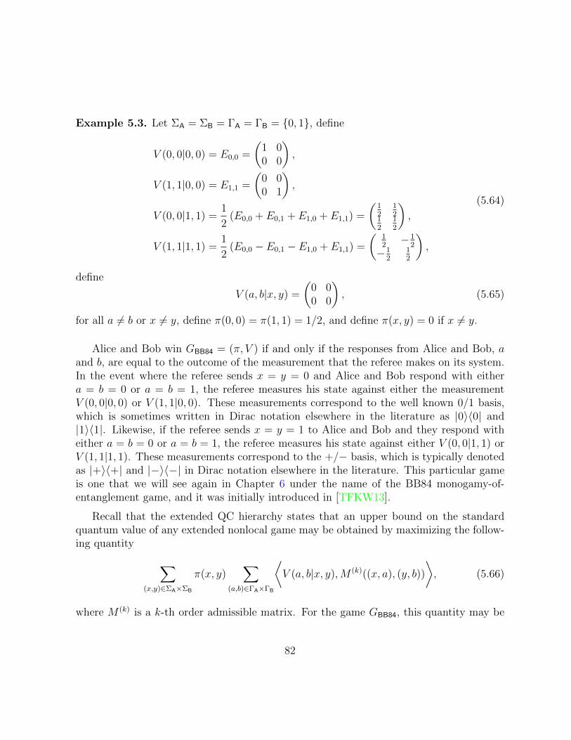
Example 5.3. Let ΣA = ΣB = ΓA = ΓB = {0, 1}, define

V (0, 0|0, 0) = E0,0 =

(1 00 0

),

V (1, 1|0, 0) = E1,1 =

(0 00 1

),

V (0, 0|1, 1) =1

2(E0,0 + E0,1 + E1,0 + E1,1) =

(12

12

12

12

),

V (1, 1|1, 1) =1

2(E0,0 − E0,1 − E1,0 + E1,1) =

(12−1

2

−12

12

),

(5.64)

define

V (a, b|x, y) =

(0 00 0

), (5.65)

for all a 6= b or x 6= y, define π(0, 0) = π(1, 1) = 1/2, and define π(x, y) = 0 if x 6= y.

Alice and Bob win GBB84 = (π, V ) if and only if the responses from Alice and Bob, aand b, are equal to the outcome of the measurement that the referee makes on its system.In the event where the referee sends x = y = 0 and Alice and Bob respond with eithera = b = 0 or a = b = 1, the referee measures his state against either the measurementV (0, 0|0, 0) or V (1, 1|0, 0). These measurements correspond to the well known 0/1 basis,which is sometimes written in Dirac notation elsewhere in the literature as |0〉〈0| and|1〉〈1|. Likewise, if the referee sends x = y = 1 to Alice and Bob and they respond witheither a = b = 0 or a = b = 1, the referee measures his state against either V (0, 0|1, 1) orV (1, 1|1, 1). These measurements correspond to the +/− basis, which is typically denotedas |+〉〈+| and |−〉〈−| in Dirac notation elsewhere in the literature. This particular gameis one that we will see again in Chapter 6 under the name of the BB84 monogamy-of-entanglement game, and it was initially introduced in [TFKW13].

Recall that the extended QC hierarchy states that an upper bound on the standardquantum value of any extended nonlocal game may be obtained by maximizing the follow-ing quantity ∑

(x,y)∈ΣA×ΣB

π(x, y)∑

(a,b)∈ΓA×ΓB

⟨V (a, b|x, y),M (k)((x, a), (y, b))

⟩, (5.66)

where M (k) is a k-th order admissible matrix. For the game GBB84, this quantity may be

82

explicitly written as

1

2

(⟨V (0, 0|0, 0),M (k)((0, 0), (0, 0))

⟩+

⟨V (1, 1|0, 0),M (k)((0, 1), (0, 1))

⟩)+

1

2

(⟨V (0, 0|1, 1),M (k)((1, 0), (1, 0))

⟩+

⟨V (1, 1|1, 1),M (k)((1, 1), (1, 1))

⟩),

(5.67)

for some level k. For simplicity, we shall just consider the first level at k = 1 of the extendedQC hierarchy for GBB84. As it turns out, and as we shall see in the coming sections, thefirst level converges to the standard quantum value, and therefore going any higher in thehierarchy will not yield any better approximations.

The software listing A.1.1 in Appendix A maximizes the objective function from equa-tion (5.66) subject to the constraints that the matrix M (1) is a first-order admissible matrix.Running the listing, one obtains the following matrix for M (1):

M (1) =

(M

(1)1,1 M

(1)1,2

M(1)2,1 M

(1)2,2

), (5.68)

where

M(1)1,1 = M

(1)2,2 =

α β+ β− α α β+ β− α αβ+ β+ 0 αβ+ αβ+ β+ 0 αβ+ αβ+

β− 0 β− αβ− αβ− 0 β− αβ− αβ−α αβ+ αβ− α 0 αβ+ αβ− α 0α αβ+ αβ− 0 α αβ+ αβ− 0 αβ+ β+ 0 αβ+ αβ+ β+ 0 αβ+ αβ+

β− 0 β− αβ− αβ− 0 β− αβ− αβ−α αβ+ αβ− α 0 αβ+ αβ− α 0α αβ+ αβ− 0 α αβ+ αβ− 0 α

,

M(1)1,2 = M

(1)2,1 =

0 0 0 γ −γ 0 0 γ −γ0 0 0 αγ −αγ 0 0 αγ −αγ0 0 0 αγ −αγ 0 0 αγ −αγ0 0 0 αγ −αγ 0 0 αγ −αγγ αγ αγ γ 0 αγ αγ γ 0−γ −αγ −αγ 0 −γ −αγ −αγ 0 −γ0 0 0 αγ −αγ 0 0 αγ −αγ0 0 0 αγ −αγ 0 0 αγ −αγγ αγ αγ γ 0 αγ αγ γ 0−γ −αγ −αγ 0 −γ −αγ −αγ 0 −γ

,

(5.69)

83

where we define the constants

α = 1/2, β± =1

8

(2±√

2), and γ =

√2

8. (5.70)

One may verify that the matrix M (1) is a first-order admissible matrix and that the equa-tion (5.67) for k = 1 yields the value of cos2(π/8) ≈ 0.8536 where

M (1)((0, 0), (0, 0)) =

(β+ 00 β−

), M (1)((0, 1), (0, 1)) =

(β− 00 β+

),

M (1)((1, 0), (1, 0)) =

(α γγ α

), M (1)((1, 1), (1, 1)) =

(α −γ−γ α

).

(5.71)

In Section 5.2, we will verify that cos2(π/8) is indeed the standard quantum value as thisvalue will also arise when calculating the lower bound of GBB84.

The CHSH extended nonlocal game

Let us now consider another game, GCHSH.

Example 5.4 (CHSH extended nonlocal game). Let ΣA = ΣB = ΓA = ΓB = {0, 1}, definea collection of measurements {V (a, b|x, y) : a ∈ ΓA, b ∈ ΓB, x ∈ ΣA, y ∈ ΣB} ⊂ Pos(R)such that

V (0, 0|0, 0) = V (0, 0|0, 1) = V (0, 0|1, 0) = E0,0,

V (1, 1|0, 0) = V (1, 1|0, 1) = V (1, 1|1, 0) = E1,1,

V (0, 1|1, 1) =1

2(E0,0 + E0,1 + E1,0 + E1,1) ,

V (1, 0|1, 1) =1

2(E0,0 − E0,1 − E1,0 + E1,1) ,

(5.72)

define

V (a, b|x, y) =

(0 00 0

)(5.73)

for all a⊕ b 6= x ∧ y, and define π(0, 0) = π(0, 1) = π(1, 0) = π(1, 1) = 1/4.

In the event that a⊕b 6= x∧y, the referee’s measurement corresponds to the zero matrixfrom equation (5.73). If instead it happens that a ⊕ b = x ∧ y, the referee then proceedsto measure with respect to one of the measurement operators from equation (5.72). This

84

winning condition is reminiscent of the standard CHSH nonlocal game. For GCHSH, wemay again consider the equation (5.66) where the quantity may be explicitly written as

1

4

(⟨V (0, 0|0, 0),M (k)((0, 0), (0, 0))

⟩+

⟨V (1, 1|0, 0),M (k)((0, 1), (0, 1))

⟩)+

1

4

(⟨V (0, 0|0, 1),M (k)((0, 0), (1, 0))

⟩+

⟨V (1, 1|0, 1),M (k)((0, 1), (1, 1))

⟩)+

1

4

(⟨V (0, 0|1, 0),M (k)((1, 0), (0, 0))

⟩+

⟨V (1, 1|1, 0),M (k)((1, 1), (0, 1))

⟩)+

1

4

(⟨V (0, 1|1, 1),M (k)((1, 0), (1, 1))

⟩+

⟨V (1, 0|1, 1),M (k)((1, 1), (1, 0))

⟩),

(5.74)

for some level k. Unlike GBB84, the first level of the extended QC hierarchy is not suffi-cient for obtaining the standard quantum value of GCHSH. Indeed, running the softwarelisting A.1.2 that implements the first level of the extended QC hierarchy yields a value of≈ 0.7578, while the non-signaling value of this game yields a value of 3/4 (refer to softwarelisting A.1.3) as does the lower bound on the standard quantum value of GCHSH. The lowerbound technique will be elaborated on further in Section 5.2.

5.2 Lower bounds for extended nonlocal games: the

see-saw method

Our lower bound heuristic for the class of extended nonlocal games is based on the work ofLiang and Doherty [LD07], where they provide a lower bound technique for Bell inequali-ties, or equivalently, nonlocal games. The primary idea of their algorithm is to note thatfixing measurements on one system yields the optimal measurements of the other systemvia an SDP. The algorithm proceeds in an iterative manner between two SDPs. In thefirst SDP, we assume that Bob’s measurements are fixed, and Alice’s measurements are tobe optimized over. In the second SDP, we take Alice’s optimized measurements from thefirst SDP and now optimize over Bob’s measurements. This method is repeated until thequantum value reaches a desired numerical precision. This “see-saw” type iteration wasdone in [WW01] by Werner and Wolf and served as a basis of inspiration for Liang andDoherty’s method. It is also worthwhile to mention that in [IIA06] the authors showedconcurrently with [LD07] that there exists an SDP that achieves a lower bound on thequantum value for a nonlocal game.

85

We must slightly adapt the Liang and Doherty lower bound algorithm to take intoaccount the actions of the referee for our extended nonlocal game. In our scenario, weshall represent Alice’s actions in terms of the residual states acting on the referee and Bobas the set {ρxa : x ∈ ΣA, a ∈ ΓA} ⊂ Pos(R⊗ B) where

ρxa = TrA ((1R ⊗ Axa ⊗ 1B) ρ) ∈ Pos(R⊗ B). (5.75)

It is then necessary and sufficient that∑

a∈ΓAρxa = τ ∈ D(R⊗ B) for all x ∈ ΣA. It then

holds that we can express the probability that Alice and Bob’s standard quantum strategywins in as ∑

(x,y)∈Σ

π(x, y)∑

(a,b)∈Γ

⟨V (a, b|x, y)⊗By

b , ρxa

⟩. (5.76)

Writing the above conditions in terms of an SDP, we have that

Lower bound SDP-1

maximize:∑

(x,y)∈Σ

π(x, y)∑

(a,b)∈Γ

⟨V (a, b|x, y)⊗By

b , ρxa

⟩subject to:

∑a∈ΓA

ρxa = τ, ∀x ∈ ΣA,

ρxa ∈ Pos(R⊗ B), ∀x ∈ ΣA, ∀a ∈ ΓA,

τ ∈ D(R⊗ B),

(5.77)

where the measurements of the referee represented as the collection {V (a, b|x, y)} as wellas the sets of measurements for Bob, represented as the collection {By

b } are fixed where thecollection of operators {ρxa} are the variables that we wish to optimize. Now we considerthe second SDP. First, observe that we can write equation (5.76) as∑

(x,y)∈Σ

π(x, y)∑

(a,b)∈Γ

⟨Φ(By

b ), ρxa⟩, (5.78)

where the mapping Φ ∈ T(B,R⊗ B) is defined as

Φ(Byb ) = π(x, y)V (a, b|x, y)⊗By

b . (5.79)

We calculate the unique adjoint mapping Φ∗ ∈ T(R⊗ B,B), as

Φ∗(ρxa) = TrR ((V (a, b|x, y)∗ ⊗ 1B) ρxa) , (5.80)

86

which may be verified from⟨Φ(By

b ), ρxa⟩

=⟨V (a, b|x, y)⊗By

b , ρxa

⟩= Tr ((V (a, b|x, y)∗ ⊗ (By

b )∗) ρxa)

= Tr ((1B ⊗ (Byb )∗) (V (a, b|x, y)∗ ⊗ 1B) ρxa)

= Tr ((Byb )∗TrR (V (a, b|x, y)∗ ⊗ 1B) ρxa)

=⟨Byb ,TrR ((V (a, b|x, y)∗ ⊗ 1B) ρxa)

⟩.

(5.81)

From this, we can define the second SDP.

Lower bound SDP-2

maximize:∑

(x,y)∈Σ

π(x, y)∑

(a,b)∈Γ

⟨Byb ,Φ

∗(ρxa)⟩

subject to:∑b∈ΓB

Byb = 1B, ∀y ∈ ΣB,

Byb ∈ Pos(B), ∀y ∈ ΣB, b ∈ ΓB.

(5.82)

While the optimization procedure is not guaranteed to converge to the actual quantumvalue, we can perform our extended QC hierarchy to check if the lower and upper boundsare in agreement to determine optimality. If this is indeed the case, we can extract theexplicit strategy that Alice and Bob perform via this lower bound method.

Bob’s measurements are given directly from the formulation of the SDP, while Alice’smeasurements may be obtained by the following equation

Axa = τ−1/2 TrB(ρxa)τ−1/2 (5.83)

for all a ∈ ΓA and x ∈ ΣA.

5.2.1 Examples: Lower-bounding the standard quantum valuesof extended nonlocal games

The BB84 extended nonlocal game

We revisit GBB84, the BB84 extended nonlocal game considered in Section 5.1.4. Weobserved that for k = 1, the extended QC hierarchy gave us a value of cos2(π/8). We

87

also claimed that this value does indeed correspond to the standard quantum value of thegame, and going any higher in the hierarchy would not yield any better approximationsto this value. In this example, we shall compute the lower bound of GBB84 and verify thatthe lower and upper bounds agree, which confirms that computing for any higher levels ofk in the extended QC hierarchy would not be useful.

The software listing A.1.4 in Appendix A computes the lower bound of GBB84 usingthe two semidefinite programs from equations (5.77) and (5.82). In the first semidefiniteprogram, we are given the measurements that the referee uses (as defined in example 6.1) aswell as some collection of measurements for Bob. When we start the see-saw algorithm, wesimply generate random unitaries of appropriate dimension to represent the measurementsthat Bob may use. These measurement operators will change as we go back and forthbetween the semidefinite programs. The variable that we are optimizing with respect to isρxa, which represents Alice’s actions.

We then plug in the variables that we obtain from the first semidefinite program intothe second semidefinite program. We repeat this process until the desired threshold isreached. In this example, the value of cos2(π/8) is obtained almost immediately, andtherefore allows one to conclude that since the upper and lower bounds are in agreement,that ω∗(GBB84) = cos2(π/8). Furthermore using equation (5.83), we can also obtain thestrategy that Alice uses to obtain this value, where the measurement operators of Aliceare given explicitly as

A00 = A1

1 =

(cos2(π/8) − sin(π/8) cos(π/8)

− sin(π/8) cos(π/8) sin2(π/8)

),

A01 = A1

0 =

(sin2(π/8) sin(π/8) cos(π/8)

sin(π/8) cos(π/8) cos2(π/8)

).

(5.84)

In this particular example, Bob’s measurement operators can take the form of any validmeasurement operators.

88

Chapter 6

Monogamy-of-Entanglement Games

In this chapter, we shall consider a particular type of extended nonlocal game referred toas a monogamy-of-entanglement game, which was initially introduced in [TFKW13].

In Section 6.1, we formally present this model and prove a number of properties aboutthis class of game. In particular, we will study the relationship between the standardquantum and unentangled strategies of certain monogamy-of-entanglement games. In Sec-tion 6.2 we will study the parallel repetition of monogamy-of-entanglement games, andin Section 6.3 we will present an example of a monogamy-of-entanglement game that Al-ice and Bob win with higher probability in the event that they use a standard quantumstrategy in place of an unentangled strategy.

This chapter is based on joint work with Nathaniel Johnston, Rajat Mittal, and JohnWatrous [JMRW16].

Contents6.1 Monogamy-of-entanglement games . . . . . . . . . . . . . . . . 90

6.1.1 Strategies and values of monogamy-of-entanglement games . . . 91

6.1.2 The BB84 monogamy-of-entanglement game . . . . . . . . . . . 93

6.1.3 Comparing standard quantum and unentangled strategies for monogamy-of-entanglement games . . . . . . . . . . . . . . . . . . . . . . . . 94

6.2 Parallel repetition of monogamy-of-entanglement games . . . 96

6.2.1 Strong parallel repetition for certain monogamy-of-entanglementgames with two questions . . . . . . . . . . . . . . . . . . . . . . 100

89

6.2.2 No strong parallel repetition for monogamy-of-entanglement gameswith non-signaling provers . . . . . . . . . . . . . . . . . . . . . . 102

6.3 Upper and lower bounds on monogamy-of-entanglement games103

6.3.1 A monogamy-of-entanglement game with quantum advantage . . 103

6.3.2 Synopsis of monogamy-of-entanglement games . . . . . . . . . . 104

6.1 Monogamy-of-entanglement games

Monogamy-of-entanglement games are a special type of extended nonlocal game, and wereoriginally introduced and studied by Tomamichel, Fehr, Kaniewski, and Wehner [TFKW13].Monogamy-of-entanglement games received their namesake as they serve as a framework toconceptualize the fundamental monogamy property exhibited by entangled qubits [CKW00].In short, this property states that for three possibly entangled qubits contained in the reg-isters X0, X1, and X2, that if Xi and Xj are maximally entangled, then Xk is completelyunentangled with qubits Xi and Xj for i 6= j 6= k where i, j, k ∈ {0, 1, 2}. This phenomenahas been studied in a number of other works [Ter01, Ter04, KW04, OV06].

The manner in which a monogamy-of-entanglement game proceeds is similar to anextended nonlocal game. After Alice and Bob supply the referee with a quantum system,we now assume that the referee selects a single question at random, and sends this samequestion to both Alice and Bob. The winning condition of a monogamy-of-entanglementgame is predicated on the ability for Alice and Bob to respond with the same answer, andthat this answer must agree with the measurement outcome of the referee.

More formally, we specify a monogamy-of-entanglement game as G = (π,R) whereπ : Σ → [0, 1] is a probability distribution defined over an alphabet Σ and where R is afunction of the form R : Γ × Σ → Pos(R) where R = Cm is a complex Euclidean spaceof dimension m belonging to the referee and where Γ is an alphabet. The function Rcorresponds to a collection of measurement operators for the referee where R(a|x) is themeasurement that corresponds to question x ∈ Σ and answer a ∈ Γ. The function R mustsatisfy ∑

a∈Γ

R(a|x) = 1R (6.1)

for every x ∈ Σ.

90

A monogamy-of-entanglement game closely follows the way in which an extended non-local game is played. First, Alice and Bob prepare a state σ ∈ D(U ⊗R⊗V) and share itwith the referee. The referee then selects a single question x ∈ Σ according to the prob-ability distribution π, and sends x to both Alice and Bob. Alice and Bob then produceand send respective responses a and b to the referee. When the referee receives a and b,it performs a measurement {R(c|x) : c ∈ Γ} on its portion of the shared state, yieldingsome measurement outcome. The game is won if and only if the measurement outcomes aand b produced by Alice and Bob agree with the outcome of the referee’s measurement. Amonogamy-of-entanglement game is depicted in Figure 6.1.

R0 R1

A

B

σx

U

V

R

x

x

a

b

Figure 6.1: A monogamy-of-entanglement game. The state σ ∈ D(U ⊗ R ⊗ V) containedin registers (U,R,V) is prepared by Alice and Bob, where R is sent to the referee and Ubelongs to Alice and V belongs to Bob. The referee selects question x according to the πdistribution, and sends x to both Alice and Bob. Alice and Bob then generate and sendanswers a and b to the referee. Alice and Bob win if and only if all measurement outcomesagree.

6.1.1 Strategies and values of monogamy-of-entanglement games

Since monogamy-of-entanglement games are a type of extended nonlocal game, one mayalso define unentangled strategies, standard quantum strategies, commuting measurementstrategies, and non-signaling strategies as considered in Chapter 3 in a similar manner.We shall define some of these strategies and their corresponding values for the case ofmonogamy-of-entanglement games explicitly.

91

For instance, a standard quantum strategy for a monogamy-of-entanglement game con-sists of finite-dimensional complex Euclidean spaces U for Alice and V for Bob, a quantumstate σ ∈ D(U ⊗R⊗ V), and two collections of measurements

{Axa : a ∈ Γ} ⊂ Pos(U) and {Bxa : a ∈ Γ} ⊂ Pos(V), (6.2)

for each x ∈ Σ. The measurement operators satisfy the constraint that∑a∈Γ

Axa = 1U and∑a∈Γ

Bxa = 1V , (6.3)

for each x ∈ Σ. For a monogamy-of-entanglement game, the winning probability for Aliceand Bob when they use a standard quantum strategy is given by∑

x∈Σ

π(x)∑a∈Γ

⟨Axa ⊗R(a|x)⊗Bx

a , σ

⟩. (6.4)

In fact, we may simplify the above expression slightly. Recall from Section 3.2.2 thatwe may assume that σ ∈ D(U ⊗ R ⊗ V) is pure for any extended nonlocal game, andthe measurements of the referee are positive semidefinite, it follows by convexity that wemay write the winning probability for Alice and Bob when they use a standard quantumstrategy as ∥∥∥∥∑

x∈Σ

π(x)∑a∈Γ

Axa ⊗R(a|x)⊗Bxa

∥∥∥∥. (6.5)

For a given monogamy-of-entanglement game G = (π,R), we write ω∗(G) to denote thestandard quantum value of G, which is the supremum winning value of Alice and Bob’swinning probability over all standard quantum strategies for G.

An unentangled strategy for a monogamy-of-entanglement game is simply a standardquantum strategy for which the state σ ∈ D(U ⊗ R ⊗ V) initially prepared by Alice andBob is fully separable. The unentangled value of a monogamy-of-entanglement game, G,can be directly derived from the unentangled value of an extended nonlocal game fromequation (3.22) as

ω(G) = maxf :Σ→Γ

∥∥∥∥∑x∈Σ

π(x)R(f(x)|x)

∥∥∥∥, (6.6)

noting again that Alice and Bob only win in a monogamy-of-entanglement game whentheir measurement outcomes agree with the measurement outcome of the referee.

92

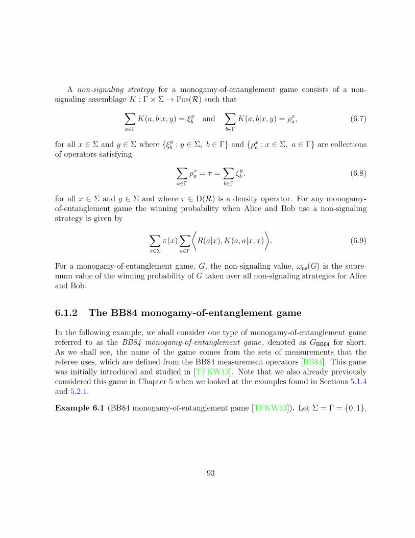
A non-signaling strategy for a monogamy-of-entanglement game consists of a non-signaling assemblage K : Γ× Σ→ Pos(R) such that∑

a∈Γ

K(a, b|x, y) = ξyb and∑b∈Γ

K(a, b|x, y) = ρxa, (6.7)

for all x ∈ Σ and y ∈ Σ where {ξyb : y ∈ Σ, b ∈ Γ} and {ρxa : x ∈ Σ, a ∈ Γ} are collectionsof operators satisfying ∑

a∈Γ

ρxa = τ =∑b∈Γ

ξyb , (6.8)

for all x ∈ Σ and y ∈ Σ and where τ ∈ D(R) is a density operator. For any monogamy-of-entanglement game the winning probability when Alice and Bob use a non-signalingstrategy is given by ∑

x∈Σ

π(x)∑a∈Γ

⟨R(a|x), K(a, a|x, x)

⟩. (6.9)

For a monogamy-of-entanglement game, G, the non-signaling value, ωns(G) is the supre-mum value of the winning probability of G taken over all non-signaling strategies for Aliceand Bob.

6.1.2 The BB84 monogamy-of-entanglement game

In the following example, we shall consider one type of monogamy-of-entanglement gamereferred to as the BB84 monogamy-of-entanglement game, denoted as GBB84 for short.As we shall see, the name of the game comes from the sets of measurements that thereferee uses, which are defined from the BB84 measurement operators [BB84]. This gamewas initially introduced and studied in [TFKW13]. Note that we also already previouslyconsidered this game in Chapter 5 when we looked at the examples found in Sections 5.1.4and 5.2.1.

Example 6.1 (BB84 monogamy-of-entanglement game [TFKW13]). Let Σ = Γ = {0, 1},

93

define

R(0|0) = E0,0 =

(1 00 0

),

R(1|0) = E1,1 =

(0 00 1

),

R(0|1) =1

2(E0,0 + E0,1 + E1,0 + E1,1) =

(12

12

12

12

),

R(1|1) =1

2(E0,0 − E0,1 − E1,0 + E1,1) =

(12−1

2

−12

12

),

(6.10)

and define π(0) = π(1) = 1/2. Then the BB84 monogamy-of-entanglement game, denotedas GBB84, is specified by GBB84 = (π,R).

In [TFKW13], the authors also showed that even if Alice and Bob adopt a standardquantum strategy for GBB84, they will perform no better than had they simply used anunentangled strategy,

ω(GBB84) = ω∗(GBB84) = cos2(π/8) ≈ 0.8536. (6.11)

That is to say, Alice and Bob gain no advantage in sharing entanglement with the referee.Recall that in Sections 5.1.4 and 5.2.1, we computed the lower and upper bound on thestandard quantum value of GBB84 and found that both values agree and are equal tocos2(π/8).

6.1.3 Comparing standard quantum and unentangled strategiesfor monogamy-of-entanglement games

Recall from Section 6.1.2 that ω(GBB84) = ω∗(GBB84), meaning that it makes no differencewhether Alice and Bob adopt a standard quantum or unentangled strategy for GBB84, asthey will win with the same probability either way. A natural question then is whether thisbehavior persists in general for the class of monogamy-of-entanglement games. Specifically,is it the case that for any monogamy-of-entanglement game, G, that

ω(G) = ω∗(G)? (6.12)

In this section, we shall show that for any monogamy-of-entanglement game wherethe size of the question set is two and the size of the answer set is arbitrary, the standard

94

quantum and unentangled values are indeed equal. However, in Section 6.3.1, we shall showthat this behavior is not true for the entire class of monogamy-of-entanglement games andpresent an explicit example of a monogamy-of-entanglement game that yields a strictlyhigher standard quantum value than unentangled value.

Theorem 6.2. Let G be any monogamy-of-entanglement game for which the question setΣ satisfies |Σ| = 2. It holds that

ω(G) = ω∗(G). (6.13)

Proof. It is evident that ω(G) ≤ ω∗(G), as this is the case for every extended nonlocalgame (and therefore every monogamy-of-entanglement game), so it remains to prove thereverse inequality. Assume without loss of generality that Σ = {0, 1}, and that G = (π,R)for π(0) = λ and π(1) = 1− λ. Consider any choice of projective measurements{

A0a : a ∈ Γ

}and

{A1a : a ∈ Γ

}(6.14)

on U for Alice and {B0a : a ∈ Γ

}and

{B1a : a ∈ Γ

}(6.15)

on V for Bob. First, note that for an optimal choice of the initial state, we can write thestandard quantum value of G in terms of the following equation

ω∗(G) =

∥∥∥∥λ∑a∈Γ

A0a ⊗R(a|0)⊗B0

a + (1− λ)∑b∈Γ

A1b ⊗R(b|1)⊗B1

b

∥∥∥∥. (6.16)

Note that the operator inside the norm of equation (6.16) is positive semidefinite since allof the measurement operators are also positive semidefinite.

Recall that for positive semidefinite operators P ∈ Pos(U) and Q ∈ Pos(V) that ifP ≤ Q then it implies that ‖P ‖ ≤ ‖Q‖. To observe this fact, note that for a positivesemidefinite operator, X, the spectral norm yields the largest eigenvalue of that operator.An equivalent way to state that X is positive semidefinite is to say that X is Hermitianwith nonnegative eigenvalues.

We can, therefore, upper bound ω∗(G) in the following way

ω∗(G) ≤∥∥∥∥λ∑

a∈Γ

A0a ⊗R(a|0)⊗ 1V + (1− λ)

∑b∈Γ

1U ⊗R(b|1)⊗B1b

∥∥∥∥. (6.17)

95

Since we enforce that the operators Axa and Byb are valid measurement operators, it holds

that ∑a∈Γ

Axa = 1U and∑b∈Γ

Byb = 1V (6.18)

for all x ∈ Σ and y ∈ Σ. Let us now replace the identity operators from equation (6.17)with these sums to obtain

ω∗(G) ≤∥∥∥∥λ∑

a,b∈Γ

A0a ⊗R(a|0)⊗B1

b + (1− λ)∑a,b∈Γ

A0a ⊗R(b|1)⊗B1

b

∥∥∥∥. (6.19)

Since {A0a ⊗ B1

b : a, b ∈ Γ} are pairwise orthogonal projections, i.e. that 〈A0a ⊗ B1

b , A0a′ ⊗

B1b′〉 = 0 for a 6= a′ and b 6= b′ and also that it holds that∥∥∥∥∑

k

Ak ⊗ Πk

∥∥∥∥ = maxk‖Ak‖ (6.20)

for a projective measurement {Πk}, we have that∥∥∥∥ ∑(a,b)∈Γ

A0a ⊗ (λR(a|0) + (1− λ)R(b|1))⊗B1

b

∥∥∥∥ ≤ maxa,b∈Γ

∥∥∥∥λR(a|0) + (1− λ)R(b|1)

∥∥∥∥. (6.21)

It follows from equation (6.6) that

ω(G) = maxa,b∈Γ

∥∥∥∥λR(a|0) + (1− λ)R(b|1)

∥∥∥∥. (6.22)

Therefore ω∗(G) ≤ ω(G).

6.2 Parallel repetition of monogamy-of-entanglement

games

For an integer r ≥ 1 and some monogamy-of-entanglement game, G, the r-fold parallelrepetition of a monogamy-of-entanglement game is when Alice and Bob play r copies ofG, denoted as Gr, wherein the referee gives the players r independent and identically

96

distributed pairs of questions simultaneously and expects a response from Alice and Bobfor each instance. The referee accepts if and only if all of the r responses satisfy thecriteria for the initial game, and rejects otherwise. The parallel repetition of a monogamy-of-entanglement game is depicted in Figure 6.2.

Define the complex Euclidean spaces R1, . . . ,Rr and define alphabets

Σ = Σ1 × · · · × Σr and Γ = Γ1 × · · · × Γr (6.23)

such that x1 ∈ Σ1, . . . , xr ∈ Σr are selected from Σ according to

πk : Σ1 × · · · × Σk → [0, 1] (6.24)

where πk(x1, . . . , xr) = π(x1) · · · π(xr). Then the r-fold parallel repetition of G starts offwith the referee accepting r registers R1, . . . ,Rr from Alice and Bob where the contents ofthe registers correspond to the state

σ ∈ D(U ⊗R1 ⊗ · · · ⊗ Rr ⊗ V), (6.25)

and selecting r questions x1 ∈ Σ, . . . , xr ∈ Σ according to π. The referee then sendsx1, . . . , xr to Alice and Bob. The players return r answers a1 ∈ Γ1, . . . , ar ∈ Γr for eachquestion. The referee then performs a measurement from the set

{R(a1, . . . , ar|x1, . . . , xr) = R(a1|x1)⊗ · · · ⊗R(ar|xr) : ai ∈ Γ, xi ∈ Σ} . (6.26)

Alice and Bob win the parallel repetition of G if and only if their answers win each of ther instances of Gr. That is, for a monogamy-of-entanglement game, Alice and Bob win ifand only if the outcomes of their measurements in every r instance of the game matcheswith the referee’s measurement outcome for every r games.

One may ask how ω(Gr) depends on ω(G) and r. It is evident that ω(Gr) ≥ ω(G)r sinceAlice and Bob can simply perform the same strategy in each instance. For any game thathas the property ω(G) = 1, it holds that ω(Gr) = 1 for any r. One may also wish to ask thequestion of how ω(Gr) scales in the event that ω(G) < 1. First note that ω(Gr) ≤ ω(G).This can be seen since, in order for the players to win all instances of the game, they mustwin the original game, G. Note also that ω(G)r ≤ ω(Gr) and ω(G)r ≤ ω(G). This holdssince the players can simply play each game independently with the optimal strategy forthe original game. We, therefore, have the following inequality relationship for the parallelrepetition of G

ω(G)r ≤ ω(Gr) ≤ ω(G). (6.27)

97

R0,1

R0,r

R1,1

R1,r

A

B

σ

R1

Rr

U

V

...

...

...

...

x1 a1

yr br

xr

b1

y1

ar

Figure 6.2: Parallel repetition of a monogamy-of-entanglement game. Alice and Bobprepare registers (R1, . . . ,Rr) and send to the referee. The referee then asks questionsx1, . . . , xr to Alice and y1, . . . , yr to Bob. Alice and Bob respond to each question withanswers a1, . . . , ar and b1, . . . , br. Once the referee receives all the answers, it performs ameasurement. Alice and Bob win the parallel repetition of the monogamy-of-entanglementgame if and only if all their answers match the referee’s measurement outcome for every rinstance.

98

It may be tempting to conclude that ω(Gr) = ω(G)r for all games, however this was surpris-ingly disproven [FRS90, Fei91, Ver96, FV02]. Specifically in [FRS90], Fortnow introduceda game G for which ω(G2) > ω(G)2. This result was later improved by Feige [Fei91], byexhibiting an example of a game where ω(G2) = ω(G) with ω(G) < 1.

We say that a game G exhibits the property of strong parallel repetition if the valueof the game raised to the r power is equal to the value of running the game r times.For instance, a monogamy-of-entanglement game, G, where the players use a standardquantum strategy satisfies strong parallel repetition if and only if

ω∗(Gr) = ω∗(G)r. (6.28)

Strong parallel repetition has been also referred to as perfect parallel repetition elsewherein the literature as in [CSUU08].

It is a fact proved in [TFKW13] that the BB84 game, GBB84, exhibits the property ofstrong parallel repetition,

ω∗(GrBB84) = ω∗(GBB84)

r =(cos2(π/8)

)r, (6.29)

where r is the number of rounds of repetition performed. A natural question for the generalclass of monogamy-of-entanglement games might be whether this behavior holds for anymonogamy-of-entanglement game. In Section 6.2.1, we prove that for any monogamy-of-entanglement game G = (π,R) where the set of measurements belonging to the referee,R, are projective, the distribution π is uniform, the size of the question set is |Σ| = 2, andthe size of the answer set is |Γ| = k for some integer k ≥ 1, then strong parallel repetitionholds.

This result of strong parallel repetition holds for the case when Alice and Bob use eitheran unentangled or a standard quantum strategy since we know from Section 6.1.3 that

ω(G) = ω∗(G) (6.30)

for any monogamy-of-entanglement game G, with |Σ| = 2 and |Γ| = k for some integerk ≥ 1. Specifically, the result that is shown in Section 6.2.1 is that

ω(Gr) = ω(G)r and ω∗(Gr) = ω∗(G)r, (6.31)

where r is the number of repetitions and G = (π,R) is a monogamy-of-entanglement where|Σ| = 2, |Γ| = k, π is uniform, and R is a collection of projective measurement operators.

While strong parallel repetition holds for a specific class of monogamy-of-entanglementgames when Alice and Bob use either an unentangled or standard quantum strategy, we

99

can ask a similar question when Alice and Bob use a non-signaling strategy instead. Aswe shall see in Section 6.2.2, it turns out that strong parallel repetition does not hold inthe non-signaling scenario. We shall illustrate this by showing a counter-example to strongparallel repetition by using a non-signaling version of the BB84 monogamy-of-entanglementgame and showing that

ωns(GrBB84) 6= ωns(GBB84)

r. (6.32)

for r = 2.

6.2.1 Strong parallel repetition for certain monogamy-of-entanglementgames with two questions

We begin this section by recalling a theorem from [TFKW13].

Theorem 6.3 (Tomamichel, Fehr, Kaniewski, and Wehner (Theorem 4 of [TFKW13])).Let G = (π,R) be a monogamy-of-entanglement game for which π is uniform over Σ, define

c(G) = maxx,y∈Σx 6=y

maxa,b∈Γ

∥∥∥∥√R(a|x)√R(b|y)

∥∥∥∥2

, (6.33)

and let Gr denote the game played r times in parallel. It holds that

ω∗(Gr) ≤(

1

|Σ| +|Σ| − 1

|Σ|√c(G)

)r. (6.34)

Equation (6.33) may be referred to as the maximal overlap of the referee’s measure-ments. As was observed in [TFKW13], this quantity satisfies

1

|Γ| ≤ c(G) ≤ 1 and c(Gr) = c(G)r. (6.35)

For any monogamy-of-entanglement game, G, Theorem 6.3 provides an upper bound onthe standard quantum value achieved when running G for r times in parallel as givenby equation (6.34). In this section, we shall show that for |Σ| = 2 that the bound fromequation (6.34) is indeed tight.

Theorem 6.4. Let G = (π,R) be a monogamy-of-entanglement game for which π is uni-form over Σ with |Σ| = 2. It holds that

ω∗(Gr) =

(1

2+

1

2

√c(G)

)r. (6.36)

100

In order to prove theorem 6.4, we first require the following proposition.

Proposition 6.5. Let G = (π,R) be a monogamy-of-entanglement game for which Σ ={0, 1}, π is uniform over Σ, and R(a|x) is a projection operator for each x ∈ Σ and a ∈ Γ.It holds that

ω(G) =1

2+

1

2maxa,b∈Γ

∥∥∥∥R(a|0)R(b|1)

∥∥∥∥. (6.37)

Proving this proposition requires the use of the following lemma.

Lemma 6.6. Let Π0 and Π1 be nonzero projection operators on Cr. It holds that∥∥Π0 + Π1

∥∥ = 1 +∥∥Π0Π1

∥∥. (6.38)

Proof. For every choice of unit vectors u0, u1 ∈ Cr, one has the formula∥∥u0u∗0 + u1u

∗1

∥∥ = 1 + |〈u0, u1〉| , (6.39)

which follows from the observation that the Hermitian operator u0u∗0 + u1u

∗1 has (at most)

two nonzero eigenvalues 1±|〈u0, u1〉|. Letting S, S0, and S1 denote the unit spheres in thespaces Cr, im(Π0), and im(Π1), respectively, one has∥∥Π0 + Π1

∥∥ = max {v∗ (Π0 + Π1) v : v ∈ S}= max

{∥∥Π0v∥∥2

+∥∥Π1v

∥∥2: v ∈ S

}= max

{|〈u0, v〉|2 + |〈u1, v〉|2 : v ∈ S, u0 ∈ S0, u1 ∈ S1

}= max {v∗ (u0u

∗0 + u1u

∗1) v : v ∈ S, u0 ∈ S0, u1 ∈ S1}

= max{∥∥u0u

∗0 + u1u

∗1

∥∥ : u0 ∈ S0, u1 ∈ S1

}= max {1 + |〈u0, u1〉| : u0 ∈ S0, u1 ∈ S1}= 1 +

∥∥Π0Π1

∥∥,

(6.40)

which proves the lemma.

Proof of Proposition 6.5. From equation (3.22), we have that the unentangled value of thegame G is given by

ω(G) = maxa,b∈Γ

∥∥∥∥ 1

2R(a|0) +

1

2R(b|1)

∥∥∥∥ =1

2maxa,b∈Γ

∥∥∥∥R(a|0) +R(b|1)

∥∥∥∥. (6.41)

101

It follows from Lemma 6.6 that ‖R(a|0) + R(b|1)‖ = 1 + ‖R(a|0)R(b|1)‖ which allows usto write equation (6.41) as

ω(G) =1

2+

1

2maxa,b∈Γ

∥∥∥∥R(a|0)R(b|1)

∥∥∥∥, (6.42)

proving the proposition.

Proof of Theorem 6.4. The upper bound

ω∗(Gr) ≤(

1

2+

1

2

√c(G)

)r, (6.43)

follows from Theorem 6.3, initially shown in [TFKW13]. Showing the other direction

ω∗(Gr) ≥(

1

2+

1

2

√c(G)

)r, (6.44)

follows from Proposition 6.5 and Lemma 6.6. The reason that this direction holds for anynumber of repetitions r is that Alice and Bob can simply play an optimal strategy for eachr games, r times in parallel. This implies that

ω∗(Gr) ≥ ω(Gr) ≥(

1

2+

1

2maxa,b∈Γ

∥∥∥∥R(a|0)R(b|1)

∥∥∥∥)r =

(1

2+

1

2

√c(G)

)r, (6.45)

which matches the upper bound from Theorem 6.3.

6.2.2 No strong parallel repetition for monogamy-of-entanglementgames with non-signaling provers

Claim 6.7 (No strong parallel repetition for non-signaling provers). There exists a monogamy-of-entanglement game, G, such that

ωns(G2) 6= ωns(G)2. (6.46)

Proof of Claim 6.7. We shall verify equation (6.46) numerically using the convex optimiza-tion software CVX [GBY08] in addition to the software listing A.1.7 in Appendix A. Theexplicit monogamy-of-entanglement game that we shall use to verify this claim is GBB84,

102

the BB84 game as mentioned in Section 6.1.2. It may be checked by running the softwarelisting A.1.7 that

ωns(G2BB84) ≈ 0.73826. (6.47)

However, we may also verify that a single repetition of GBB84 is cos2(π/8), that is

ωns(GBB84) = cos2(π/8). (6.48)

From this, it is clear that

ωns(G2BB84) 6= ωns(GBB84)

2 = cos4(π/8), (6.49)

which concludes the proof.

6.3 Upper and lower bounds on

monogamy-of-entanglement games

In this section, we apply the upper and lower bound techniques for extended nonlocalgames from Chapter 5, and apply them to monogamy-of-entanglement games. In doing so,we are able to verify the existence of a monogamy-of-entanglement game where Alice andBob perform better if they use a standard quantum strategy as opposed to an unentangledone.

6.3.1 A monogamy-of-entanglement game withquantum advantage

Example 6.8 (A monogamy-of-entanglement game with quantum advantage). Let ζ =exp(2πi

3) and consider the following four mutually unbiased bases:

B0 = {e0, e1, e2} ,

B1 =

{e0 + e1 + e2√

3,e0 + ζ2e1 + ζe2√

3,e0 + ζe1 + ζ2e2√

3

},

B2 =

{e0 + e1 + ζe2√

3,e0 + ζ2e1 + ζ2e2√

3,e0 + ζe1 + e2√

3

},

B3 =

{e0 + e1 + ζ2e2√

3,e0 + ζ2e1 + e2√

3,e0 + ζe1 + ζe2√

3

}.

(6.50)

103

Define a monogamy-of-entanglement game G = (π,R) so that

π(0) = π(1) = π(2) = π(3) =1

4(6.51)

and R is such that

{R(0|x), R(1|x), R(2|x)} (6.52)

represents a measurement with respect to the basis Bx, for each x ∈ {0, 1, 2, 3}. In orderto observe that ω(G) < ω∗(G), first consider the following unentangled strategy. Alice andBob prepare the state

u =

(1− i

√3

4

)e0 +

(1 + i

√3

5

)e1 +

(1 +

3√5

)e2, (6.53)

and sends it to the referee. In the event that x = 0 or x = 1, Alice and Bob respond witha = b = 2. If instead x = 2 or x = 3, Alice and Bob respond with a = b = 0. The value ofthe game in this case is given by

ω(G) =1

4

⟨R(2|0) +R(2|1) +R(0|2) +R(0|3), ρ

⟩=

3 +√

5

8≈ 0.6545, (6.54)

where ρ = uu∗ ∈ D(R ⊗ A ⊗ B). An exhaustive search over all unentangled strategiesreveals that equation (6.54) is optimal. In contrast, a computer search over quantumstrategies using the lower bound techniques from Sectionf 5.2 has revealed that

ω∗(G) ≥ 0.660986, (6.55)

which is strictly larger than the unentangled value of this game. This strategy is availablefor download from the software repository [JR15] and is also provided as a software examplein Appendix A. It is uncertain what the optimal standard quantum strategy is for this game,but the value of such a strategy is bounded as follows

2/3 ≥ ω∗(G) ≥ 0.660986. (6.56)

6.3.2 Synopsis of monogamy-of-entanglement games

The following table gives an overview of what is currently known about the class ofmonogamy-of-entanglement games and summarizes some of the main contributions of thischapter.

1So long as the measurements used by the referee are projective and the probability distribution, π,from which the questions are asked is uniform.

104

Inputs (|Σ|) Outputs (|Γ|) ω∗(G) = ω(G) ω∗(Gr) = ω∗(G)r ωns(Gr) = ωns(G)r

2 ≥ 1 yes yes1 no

3 ≥ 1 ? ? no

4 3 no ? no

Table 6.1: A table of known results for monogamy-of-entanglement games. The first andsecond column refer to the number of inputs and outputs for such a game. The thirdcolumn states whether or not the unentangled and standard quantum values are equal,and the last two columns state whether or not strong parallel repetition holds with eitherquantum players or non-signaling players respectively.

105

Chapter 7

Conclusions and open problems

In this thesis, we have laid the foundation for the extended nonlocal game model, a supersetof the nonlocal game model where the referee also holds a quantum system.

In Chapter 3 we defined and analyzed the analogous types of strategies and corre-sponding game values (standard quantum, unentangled, commuting measurement, andnon-signaling) that the players, Alice and Bob, can make use of in such a game.

In Chapter 4, we took a deeper look at the extended nonlocal game model and showedthat there exists an example of an extended nonlocal game where if the dimension ofAlice and Bob’s shared quantum system is finite, then the standard quantum value willbe strictly less than 1. However, taking the limit as the dimension tends to infinity,the standard quantum value approaches 1. We saw how this result implies somethingnon-trivial about tripartite steering inequalities, specifically that there exists a tripartitesteering inequality for which an infinite-dimensional state is required in order to maximallyviolate the inequality.

In Chapter 5, we provided a technique to place upper bounds on the standard quantumvalue of an extended nonlocal game that generalizes the QC hierarchy, which we referredto as the extended QC hierarchy. We have shown that the hierarchy enjoys many of thesame useful properties that the original QC hierarchy does, specifically, convergence tothe set of commuting measurement assemblages. We also adapted the techniques of Liangand Doherty [LD07] to place lower bounds on the standard quantum value of extendednonlocal games. Furthermore, we have also presented software that calculates lower andupper bounds using these techniques of certain special classes of extended nonlocal games.

In Chapter 6, we took these tools and analyzed the class of monogamy-of-entanglementgames, a class of games that were initially studied in the context of position-based cryp-

106

tography [TFKW13]. We proved a number of properties that these games have includinghow they behave under parallel repetition, how entanglement may help in Alice and Bob’sstrategies, etc.

A number of questions regarding the class of monogamy-of-entanglement games remainopen. Specifically,

Question 7.1. Other examples of monogamy-of-entanglement games where ω(G) <ω∗(G).

The complete landscape of how the quantum and classical values compare for differ-ent instances of monogamy-of-entanglement games is something to be explored. We onlyknow of a small number of isolated examples where ω(G) < ω∗(G) for a monogamy-of-entanglement game, G.

In Section 6.3.1 a set of |Σ| = 4 mutually unbiased bases in |Γ| = 3 dimensions allowAlice and Bob to perform better if they adopt a standard quantum strategy instead of anunentangled strategy. This is the smallest example of a monogamy-of-entanglement gamethat was found having this property. Is there an example having fewer questions or feweranswers? This example would have to have at least three questions, since we know thatfor |Σ| = 2, that the unentangled and standard quantum values agree for any numberof outputs as shown in Section 6.1.3. Numerical results indicate that the monogamy-of-entanglement game consisting of |Σ| = 3 where the referee’s measurements are defined interms of mutually unbiased bases gives no such separation. Is it possible that anothermonogamy-of-entanglement game with |Σ| = 3 questions exists where such a separationbetween unentangled and standard quantum values exists?

One brute force method that can be used to check if there exists a monogamy-of-entanglement game for |Σ| = 3 where a standard quantum strategy will outperform anunentangled strategy is to run a computer search over randomly generated instances ofsuch monogamy-of-entanglement games. The software provided in the Appendix of thisthesis A as well as hosted on the software repository [Rus15] provides a suite of tools thatgive upper and lower bounds on the quantum value (as described in Chapter 5) as well astools for calculating the unentangled value of any monogamy-of-entanglement game. Oneapproach would be to randomly generate monogamy-of-entanglement games where |Σ| = 3and |Γ| ≥ 2, and see if any example of such games yield ω(G) < ω∗(G). This approachdoes not seem particularly promising, as if such a game were to exist with this property,it most likely has a very specific structure that would be difficult to capture by randomgeneration.

107

On a related note, under what conditions does a monogamy-of-entanglement gamebased on mutually unbiased bases admit a standard quantum over unentangled strategyadvantage? Numerically, it may be checked that a monogamy-of-entanglement game con-sisting |Σ| = 5 and |Γ| = 4 also yields a standard quantum advantage over any unentangledstrategy. Does this behavior persist for any monogamy-of-entanglement game defined bymutually unbiased bases as long as the number of inputs is at least |Σ| = 4, and thenumber of outputs is at least |Γ| = 3? Furthermore, do there exist other monogamy-of-entanglement games where |Σ| ≥ 4 and |Γ| ≥ 3 such that ω(G) < ω∗(G)? Just as acomputer search can be constructed where |Σ| = 3 and |Γ| ≥ 2, one may also formulate asearch that checks for larger instances as well.

Question 7.2. Parallel repetition for monogamy-of-entanglement games?

It was shown in Section 6.2.1 (Theorem 6.3) that for any monogamy-of-entanglementgame defined in terms of projective measurements for the referee where |Σ| = 2 and |Γ| ≥ kfor some integer k ≥ 1 that strong parallel repetition holds. Would it be possible to extendfrom projective measurements to non-projective measurements, such as POVMs? Aftersimulating approximately 108 random instances of monogamy-of-entanglement games with|Σ| = 2 defined in terms of POVMs, all games were found to obey strong parallel repetitionfor r = 2 rounds of repetition.

Furthermore, the claim that strong parallel repetition holds for monogamy-of-entanglementgames where the measurements of the referee are projective and |Σ| = 2 assumes thatthe questions that the referee asks are selected uniformly at random. Is it possible thatthe strong parallel repetition property will continue to hold despite the distribution ofquestions? If indeed it does hold under nonuniform distributions, the bound from equa-tion (6.34) from Theorem 6.3 will most likely be in a more complicated form. Ultimately,the overall goal for parallel repetition of monogamy-of-entanglement games would be toeither prove or disprove strong parallel repetition for the entire class of such games.

There also exists other questions and directions for further research.

Question 7.3. Other examples of using extended nonlocal games to study tripartite steer-ing.

As mentioned in Chapter 4, we were able to prove a non-trivial statement about acertain type of tripartite steering using the extended nonlocal game model. Given the con-nection between extended nonlocal games and tripartite steering, are there other possiblequestions we can answer that become more apparent using the extended nonlocal gamemodel?

108

Question 7.4. Does there exist a nonlocal game G such that ω∗(G) = 1 and that ω∗N(G) <1 for every positive integer N?

As mentioned in Chapter 4, it is known that nonlocal games with quantum questionsand quantum answers do satisfy the above property [LTW13]. However, it is unknown fornonlocal games with classical questions and classical answers. This question is most likelydifficult to solve.

109

References

[AJR15] Srinivasan Arunachalam, Nathaniel Johnston, and Vincent Russo. Is abso-lute separability determined by the partial transpose? Quantum Information& Computation, 15(7&8):0694–0720, 2015. 4

[AMR13] Srinivasan Arunachalam, Abel Molina, and Vincent Russo. Quantum hedg-ing in two-round prover-verifier interactions. arXiv preprint arXiv:1310.7954,2013. 5

[Bab85] Laszlo Babai. Trading group theory for randomness. In Proceedings of theseventeenth annual ACM symposium on Theory of computing, pages 421–429. ACM, 1985. 24

[BB84] Charles Bennett and Gilles Brassard. Quantum cryptography: Public keydistribution and coin tossing. Proceedings of IEEE International Conferenceon Computers, Systems and Signal Processing, 175, 1984. 93

[BBC+93] Charles Bennett, Gilles Brassard, Claude Crepeau, Richard Jozsa, AsherPeres, and William Wootters. Teleporting an unknown quantum state viadual classical and Einstein-Podolsky-Rosen channels. Physical review letters,70(13):1895, 1993. 23

[BBT05] Gilles Brassard, Anne Broadbent, and Alain Tapp. Quantum pseudo-telepathy. Foundations of Physics, 35(11):1877–1907, 2005. 2, 24

[BCJ+15] Somshubhro Bandyopadhyay, Alessandro Cosentino, Nathaniel Johnston,Vincent Russo, John Watrous, and Nengkun Yu. Limitations on separablemeasurements by convex optimization. IEEE Transactions on InformationTheory, 61(15142258):3593–3604, 2015. doi:10.1109/TIT.2015.2417755.4

110

[BCP+14] Nicolas Brunner, Daniel Cavalcanti, Stefano Pironio, Valerio Scarani, andStephanie Wehner. Bell nonlocality. Reviews of Modern Physics, 86(2):419,2014. 32

[Bel64] John Bell. On the Einstein-Podolsky-Rosen paradox. Physics, 1(3):195–200,1964. 24

[BFL91] Laszlo Babai, Lance Fortnow, and Carsten Lund. Non-deterministic expo-nential time has two-prover interactive protocols. Computational Complexity,1(1):3–40, 1991. 24

[BFS13] Harry Buhrman, Serge Fehr, and Christian Schaffner. On the parallelrepetition of multi-player games: The no-signaling case. arXiv preprintarXiv:1312.7455, 2013. 2, 24

[BOGKW88] Michael Ben-Or, Shafi Goldwasser, Joe Kilian, and Avi Wigderson. Multi-prover interactive proofs: How to remove intractability assumptions. In Pro-ceedings of the Twentieth Annual ACM Symposium on Theory of Computing,pages 113–131. ACM, 1988. 24

[Bus12] Francesco Buscemi. All entangled quantum states are nonlocal. Physicalreview letters, 108(20):200401, 2012. 44, 45

[BV04] Stephen Boyd and Lieven Vandenberghe. Convex optimization. Cambridgeuniversity press, 2004. 3, 6

[CG04] Daniel Collins and Nicolas Gisin. A relevant two qubit Bell inequality in-equivalent to the CHSH inequality. Journal of Physics A: Mathematical andGeneral, 37(5):1775, 2004. 72

[CHSH69] John Clauser, Michael Horne, Abner Shimony, and Richard Holt. Proposedexperiment to test local hidden-variable theories. Physical Review Letters,23(15):880, 1969. 24

[CHTW04] Richard Cleve, Peter Hoyer, Benjamin Toner, and John Watrous. Conse-quences and limits of nonlocal strategies. In Computational Complexity,2004. Proceedings. 19th IEEE Annual Conference on, pages 236–249. IEEE,2004. 2, 24

[CKW00] Valerie Coffman, Joydip Kundu, and William Wootters. Distributed entan-glement. Physical Review A, 61(5):052306, 2000. 90

111

[CM14] Richard Cleve and Rajat Mittal. Characterization of binary constraint sys-tem games. In Javier Esparza, Pierre Fraigniaud, Thore Husfeldt, and EliasKoutsoupias, editors, Automata, Languages, and Programming, volume 8572of Lecture Notes in Computer Science, pages 320–331. Springer Berlin Heidel-berg, 2014. URL: http://dx.doi.org/10.1007/978-3-662-43948-7_27,doi:10.1007/978-3-662-43948-7_27. 2, 24

[CR14] Alessandro Cosentino and Vincent Russo. Small sets of locally indistin-guishable orthogonal maximally entangled states. Quantum Information &Computation, 14(13-14):1098–1106, 2014. 4

[CSA+15] Daniel Cavalcanti, Paul Skrzypczyk, Gregory Aguilar, Ranieri Nery,Paulo Souto Ribeiro, and Stephen Walborn. Detection of entanglement inasymmetric quantum networks and multipartite quantum steering. NatureCommunications, 6(7941), 2015. doi:doi:10.1038/ncomms8941. 34, 62

[CSUU08] Richard Cleve, William Slofstra, Falk Unger, and Sarvagya Upadhyay. Per-fect parallel repetition theorem for quantum XOR proof systems. Computa-tional Complexity, 17(2):282–299, 2008. 2, 24, 32, 99

[CV15] Matthew Coudron and Thomas Vidick. Interactive proofs with approxi-mately commuting provers. In Automata, Languages, and Programming,pages 355–366. Springer, 2015. 2

[DLTW08] Andrew Doherty, Yeong-Cherng Liang, Ben Toner, and Stephanie Wehner.The quantum moment problem and bounds on entangled multi-prover games.In Computational Complexity, 2008. CCC’08. 23rd Annual IEEE Conferenceon, pages 199–210. IEEE, 2008. 2, 24, 30, 32, 66, 67

[DSV13] Irit Dinur, David Steurer, and Thomas Vidick. A parallel repetition theo-rem for entangled projection games. Computational Complexity, 24:201–254,2013. doi:10.1007/s00037-015-0098-3. 2, 24

[Fei91] Uriel Feige. On the success probability of the two provers in one-round proofsystems. In Structure in Complexity Theory Conference, 1991., Proceedingsof the Sixth Annual, pages 116–123. IEEE, 1991. 24, 99

[FK94] Uri Feige and Joe Kilian. Two prover protocols: Low error at affordable rates.In Proceedings of the Twenty-sixth Annual ACM Symposium on Theory ofComputing, pages 172–183. ACM, 1994. 24

112

[For89] Lance Fortnow. Complexity-theoretic aspects of interactive proof systems.PhD thesis, Massachusetts Institute of Technology, 1989. 24

[Fri12] Tobias Fritz. Tsirelson’s problem and Kirchberg’s conjecture. Reviews inMathematical Physics, 24(05):1250012, 2012. 34

[FRS90] Lance Fortnow, John Rompel, and Michael Sipser. Errata for on the powerof multi-prover interactive protocols. In Structure in Complexity TheoryConference, pages 318–319, 1990. 99

[FV02] Uriel Feige and Oleg Verbitsky. Error reduction by parallel repetitiona neg-ative result. Combinatorica, 22(4):461–478, 2002. 99

[GBY08] Michael Grant, Stephen Boyd, and Yinyu Ye. CVX: MATLAB software fordisciplined convex programming, 2008. 75, 102, 118

[GKMR14] David Gosset, Vadym Kliuchnikov, Michele Mosca, and Vincent Russo. Analgorithm for the T-count. Quantum Information & Computation, 14(15-16):1261–1276, 2014. 4

[GMR85] Shafi Goldwasser, Silvio Micali, and Charles Rackoff. The knowledge com-plexity of interactive proof-systems. In Proceedings of the seventeenth annualACM symposium on Theory of computing, pages 291–304. ACM, 1985. 24

[IIA06] Tsuyoshi Ito, Hiroshi Imai, and David Avis. Bell inequalities stronger thanthe Clauser-Horne-Shimony-Holt inequality for three-level isotropic states.Physical Review A, 73(4):042109, 2006. 85

[JMRW16] Nathaniel Johnston, Rajat Mittal, Vincent Russo, and John Watrous. Ex-tended nonlocal games and monogamy-of-entanglement games. Proc. R. Soc.A, 2016, 472, 20160003, 2016. 4, 34, 67, 89

[Joh15] Nathaniel Johnston. QETLAB: MATLAB software for quantum entangle-ment. http://www.qetlab.com, 2015. 118

[JP11] Marius Junge and Carlos Palazuelos. Large violation of Bell inequalities withlow entanglement. Communications in Mathematical Physics, 306(3):695–746, 2011. 2, 24

[JR15] Nathaniel Johnston and Vincent Russo. Supplementary software for im-plementing the examples for the extended QC hierarchy of semidefinite

113

programs. https://github.org/vprusso/monogamy-of-entanglement-games,2015. 104

[KGN15] Hirotada Kobayashi, Francois Le Gall, and Harumichi Nishimura. General-ized quantum Arthur-Merlin games. pages 488–511, 2015. 64

[KKM+11] Julia Kempe, Hirotada Kobayashi, Keiji Matsumoto, Ben Toner, andThomas Vidick. Entangled games are hard to approximate. SIAM Jour-nal on Computing, 40(3):848–877, 2011. 2, 24

[KLM07] Phillip Kaye, Raymond Laflamme, and Michele Mosca. An Introduction toQuantum Computing. Oxford University Press, 2007. 6

[KR10] Julia Kempe and Oded Regev. No strong parallel repetition with entangledand non-signaling provers. In Computational Complexity (CCC), 2010 IEEE25th Annual Conference on, pages 7–15. IEEE, 2010. 2, 24

[KRT10] Julia Kempe, Oded Regev, and Ben Toner. Unique games with entangledprovers are easy. SIAM Journal on Computing, 39(7):3207–3229, 2010. 2, 24

[KW04] Masato Koashi and Andreas Winter. Monogamy of quantum entanglementand other correlations. Physical Review A, 69(2):022309, 2004. 90

[LD07] Yeong-Cherng Liang and Andrew Doherty. Bounds on quantum correlationsin Bell-inequality experiments. Physical Review A, 75(4):042103, 2007. 2, 3,66, 85, 106

[LTW13] Debbie Leung, Ben Toner, and John Watrous. Coherent state exchange inmulti-prover quantum interactive proof systems. Chicago Journal of Theo-retical Computer Science, 11:1–18, 2013. 48, 109

[NC00] Michael Nielsen and Isaac Chuang. Quantum computation and quantuminformation. Cambridge university press, 2000. 3, 6, 24

[NPA07] Miguel Navascues, Stefano Pironio, and Antonio Acın. Bound-ing the set of quantum correlations. Physical Review Letters,98:010401, 2007. URL: http://link.aps.org/doi/10.1103/PhysRevLett.98.010401, doi:10.1103/PhysRevLett.98.010401. 2, 32, 66, 67, 73

[NPA08] Miguel Navascues, Stefano Pironio, and Antonio Acın. A convergent hierar-chy of semidefinite programs characterizing the set of quantum correlations.New Journal of Physics, 10(7):073013, 2008. 32, 66, 67, 73, 75, 78

114

[OV06] Tobias Osborne and Frank Verstraete. General monogamy inequality forbipartite qubit entanglement. Physical Review Letters, 96(22):220503, 2006.90

[Pau03] Vern Paulsen. Completely bounded maps and operator algebras. CambridgeUniversity Press, 2003. 39

[PV09] Karoly Pal and Tamas Vertesi. Quantum bounds on Bell inequalities. Phys-ical Review A, 79(2):022120, 2009. 62, 67, 72

[Raz98] Ran Raz. A parallel repetition theorem. SIAM Journal on Computing,27(3):763–803, 1998. 24

[Rud91] Walter Rudin. Functional analysis. McGraw-Hill, Inc., 1991. 17

[Rus] Vincent Russo. Supplementary software for thesis.https://github.com/vprusso/phd thesis. 119

[Rus15] Vincent Russo. Supplementary software for extended nonlocal games.https://github.org/vprusso/extended-nonlocal-games, 2015. 4, 107

[Rus16] Vincent Russo. Supplementary software for monogamy-of-entanglementgames. https://github.com/vprusso/nonlocal games seminar talk, 2016. 4

[RV15] Oded Regev and Thomas Vidick. Quantum XOR games. In ACM Transac-tions on Computation Theory, volume 4, page 15. IEEE, 2015. 2, 24, 44, 45,47, 48, 61

[RW16] Vincent Russo and John Watrous. Extended nonlocal games from quantum-classical games. 2016. 4, 45

[SBC+15] Ana Belen Sainz, Nicolas Brunner, Daniel Cavalcanti, Paul Skrzypczyk,and Tamas Vertesi. Postquantum steering. Physical review letters,115(19):190403, 2015. 34, 62

[Ter01] Barbara Terhal. A family of indecomposable positive linear maps based onentangled quantum states. Linear Algebra and its Applications, 323(1):61–73, 2001. 90

[Ter04] Barbara Terhal. Is entanglement monogamous? IBM Journal of Researchand Development, 48(1):71–78, 2004. 90

115

[TFKW13] Marco Tomamichel, Serge Fehr, Jkedrzej Kaniewski, and Stephanie Wehner.A monogamy-of-entanglement game with applications to device-independentquantum cryptography. New Journal of Physics, 15(10):103002, 2013. 2, 82,89, 90, 93, 94, 99, 100, 102, 107

[Ver96] Oleg Verbitsky. Towards the parallel repetition conjecture. Theoretical Com-puter Science, 157(2):277–282, 1996. 99

[Vid13] Thomas Vidick. Three-player entangled XOR games are NP-hard to ap-proximate. In Foundations of Computer Science (FOCS), 2013 IEEE 54thAnnual Symposium on, pages 766–775. IEEE, 2013. 2, 24

[Wat04] John Watrous. Theory of quantum information lecture notes, lecture 7.published electronically at http://www.cs.uwaterloo.ca/ watrous/lecture-notes.html, 2004. 3, 18

[Wat15] John Watrous. Theory of Quantum Information. 2015. 3, 6

[Wil13] Mark Wilde. Quantum information theory. Cambridge University Press,2013. 6, 24

[WW01] Reinhard Werner and Michael Wolf. Bell inequalities and entanglement.Quantum Information & Computation, 1(3):1–25, 2001. 85

116

APPENDICES

117

Appendix A

Software

Setup

Requirements

• MATLAB,

• CVX ≥ 2.1 [GBY08],

• QETLAB ≥ 0.8 [Joh15].

List of functions

• MonogamyGameValueUB (by N. Johnston) — Given a monogamy-of-entanglement game,G, the function calculates an upper bound on the quantum value of G;

• MonogamyGameValueLB — Given a monogamy-of-entanglement game, G, the functioncalculates an lower bound on the quantum value of G;

• MUB (by N. Johnston) — generates a set of mutually unbiased bases for a givendimension;

118

A.1 Software Listings

All of the following software listings in this Appendix are hosted on the Github repositoryfound here [Rus].

A.1.1 The first level of the extended QC hierarchy for the BB84extended nonlocal game

e0 = [1;0]; e1 = [0;1]; ep = [1;1]/sqrt(2); em = [1;-1]/sqrt(2);

psi0_dm = e0*e0’; psi0_dmc = e1*e1’;

psi1_dm = ep*ep’; psi1_dmc = em*em’;

R00 = psi0_dm/2;

R01 = psi0_dmc/2;

R10 = psi1_dm/2;

R11 = psi1_dmc/2;

dim = 9;

A00_B00 = zeros(dim); A01_B01 = zeros(dim);

A10_B10 = zeros(dim); A11_B11 = zeros(dim);

% These are the relative positions of these

% entries as indexed by strings in the matrix.

A00_B00(2,6) = 1; A00_B00(6,2) = 1;

A01_B01(3,7) = 1; A01_B01(7,3) = 1;

A10_B10(4,8) = 1; A10_B10(8,4) = 1;

A11_B11(5,9) = 1; A11_B11(9,5) = 1;

A = 1/2*( kron(R00, A00_B00) + kron(R01, A01_B01) ) + ...

1/2*( kron(R10, A10_B10) + kron(R11,A11_B11) );

cvx_begin sdp

cvx_precision best

%#ok<*VUNUS> % suppress MATLAB warnings for equality checks in CVX

%#ok<*EQEFF> % suppress MATLAB warnings for inequality checks in CVX

% Admissible matrix

119

variable M(2*dim,2*dim) hermitian

% Sub-block matrices found in the admissible matrix

variable M11(dim,dim)

variable M12(dim,dim)

variable M21(dim,dim)

variable M22(dim,dim)

M == [ M11 M12;

M21 M22 ];

maximize trace( A*M )

subject to

% Normalization condition:

M11(1,1) + M22(1,1) == 1;

for i = 1:dim

for j = 1:dim

% Ensure commutation relation holds

%(i.e. [A,B] = 0)

M11(i,j) == M11(j,i);

M12(i,j) == M12(j,i);

M21(i,j) == M21(j,i);

M22(i,j) == M22(j,i);

% Enforce operators as projective measurements

% (i.e. the square of the same operator is found in the top

% column / row of the diagonal entry).

M11(i,i) == M11(1,i);

M11(i,i) == M11(i,1);

M12(i,i) == M12(1,i);

M12(i,i) == M12(i,1);

M21(i,i) == M21(1,i);

120

M21(i,i) == M21(i,1);

M22(i,i) == M22(1,i);

M22(i,i) == M22(i,1);

end

end

% Enforce that projective measurements sum to 1:

for i = 1:dim

for j = 1:dim

if mod(i,2) == 0

M11(i,j) + M11(i+1,j) == M11(1,j);

M12(i,j) + M12(i+1,j) == M12(1,j);

M21(i,j) + M21(i+1,j) == M21(1,j);

M22(i,j) + M22(i+1,j) == M22(1,j);

end

if mod(j,2) == 0

M11(i,j) + M11(i,j+1) == M11(i,1);

M12(i,j) + M12(i,j+1) == M12(i,1);

M21(i,j) + M21(i,j+1) == M21(i,1);

M22(i,j) + M22(i,j+1) == M22(i,1);

end

end

end

% Ensure that the matrix is PSD.

M >= 0;

cvx_end

cvx_optval =

0.8536

A.1.2 The first level of the extended QC hierarchy for the CHSHextended nonlocal game

e0 = [1;0]; e1 = [0;1]; ep = [1;1]/sqrt(2); em = [1;-1]/sqrt(2);

121

psi0_dm = e0*e0’; psi0_dmc = e1*e1’;

psi1_dm = ep*ep’; psi1_dmc = em*em’;

R00 = psi0_dm/2;

R01 = psi0_dmc/2;

R10 = psi1_dm/2;

R11 = psi1_dmc/2;

dim = 9;

A00_B00 = zeros(dim); A01_B01 = zeros(dim);

A10_B10 = zeros(dim); A11_B11 = zeros(dim);

% These are the relative positions of these entries as

% indexed by strings in the matrix.

A00_B00(2,6) = 1; A00_B00(6,2) = 1;

A01_B01(3,7) = 1; A01_B01(7,3) = 1;

A10_B10(4,8) = 1; A10_B10(8,4) = 1;

A11_B11(5,9) = 1; A11_B11(9,5) = 1;

A00_B00 = zeros(dim); A01_B01 = zeros(dim);

A00_B10 = zeros(dim); A01_B11 = zeros(dim);

A10_B00 = zeros(dim); A11_B01 = zeros(dim);

A10_B11 = zeros(dim); A11_B10 = zeros(dim);

A00_B00(2,6) = 1; A00_B00(6,2) = 1;

A00_B10(2,8) = 1; A00_B10(8,2) = 1;

A01_B01(3,7) = 1; A01_B01(7,3) = 1;

A01_B11(3,9) = 1; A01_B11(9,3) = 1;

A10_B00(4,6) = 1; A10_B00(6,4) = 1;

A10_B11(4,9) = 1; A10_B11(9,4) = 1;

A11_B01(5,7) = 1; A11_B01(7,5) = 1;

A11_B10(5,8) = 1; A11_B10(8,5) = 1;

122

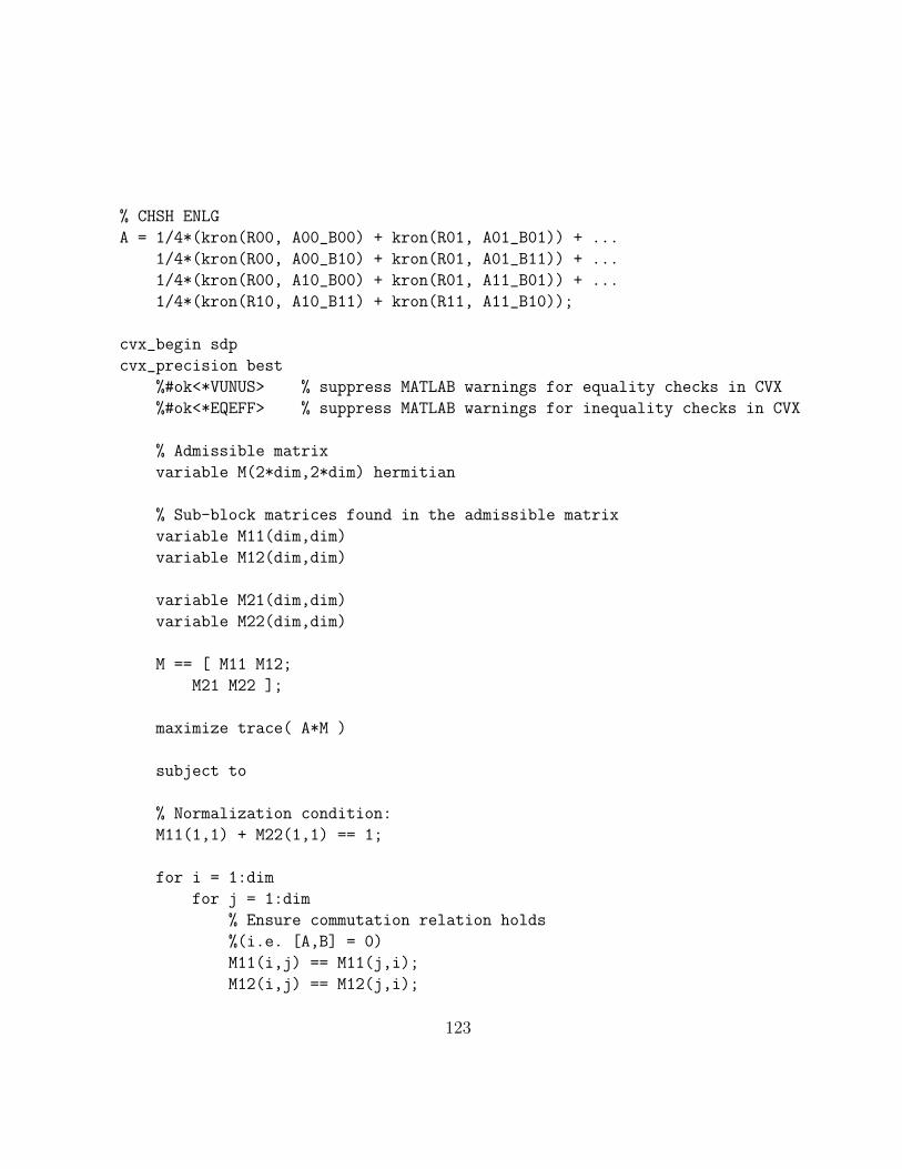
% CHSH ENLG

A = 1/4*(kron(R00, A00_B00) + kron(R01, A01_B01)) + ...

1/4*(kron(R00, A00_B10) + kron(R01, A01_B11)) + ...

1/4*(kron(R00, A10_B00) + kron(R01, A11_B01)) + ...

1/4*(kron(R10, A10_B11) + kron(R11, A11_B10));

cvx_begin sdp

cvx_precision best

%#ok<*VUNUS> % suppress MATLAB warnings for equality checks in CVX

%#ok<*EQEFF> % suppress MATLAB warnings for inequality checks in CVX

% Admissible matrix

variable M(2*dim,2*dim) hermitian

% Sub-block matrices found in the admissible matrix

variable M11(dim,dim)

variable M12(dim,dim)

variable M21(dim,dim)

variable M22(dim,dim)

M == [ M11 M12;

M21 M22 ];

maximize trace( A*M )

subject to

% Normalization condition:

M11(1,1) + M22(1,1) == 1;

for i = 1:dim

for j = 1:dim

% Ensure commutation relation holds

%(i.e. [A,B] = 0)

M11(i,j) == M11(j,i);

M12(i,j) == M12(j,i);

123

M21(i,j) == M21(j,i);

M22(i,j) == M22(j,i);

% Enforce operators as projective measurements

% (i.e. the square of the same operator is found in the top

% column / row of the diagonal entry).

M11(i,i) == M11(1,i);

M11(i,i) == M11(i,1);

M12(i,i) == M12(1,i);

M12(i,i) == M12(i,1);

M21(i,i) == M21(1,i);

M21(i,i) == M21(i,1);

M22(i,i) == M22(1,i);

M22(i,i) == M22(i,1);

end

end

% Enforce that projective measurements sum to 1:

for i = 1:dim

for j = 1:dim

if mod(i,2) == 0

M11(i,j) + M11(i+1,j) == M11(1,j);

M12(i,j) + M12(i+1,j) == M12(1,j);

M21(i,j) + M21(i+1,j) == M21(1,j);

M22(i,j) + M22(i+1,j) == M22(1,j);

end

if mod(j,2) == 0

M11(i,j) + M11(i,j+1) == M11(i,1);

M12(i,j) + M12(i,j+1) == M12(i,1);

M21(i,j) + M21(i,j+1) == M21(i,1);

M22(i,j) + M22(i,j+1) == M22(i,1);

end

end

end

124

% Ensure that the matrix is PSD.

M >= 0;

cvx_end

cvx_optval =

0.75783

A.1.3 The non-signaling value for the CHSH extended nonlocalgame

n = 1;

dim = 2^n;

e0 = [1;0]; e1 = [0;1];

ep = [1;1]/sqrt(2); em = [1;-1]/sqrt(2);

eip = (e0 + 1j*e1)/sqrt(2); eim = (e0 - 1j*e1)/sqrt(2);

psi0_dm = e0*e0’; psi0_dmc = e1*e1’;

psi1_dm = ep*ep’; psi1_dmc = em*em’;

psi2_dm = eip*eip’; psi2_dmc = eim*eim’;

P = zeros(2,2,2,2);

%P(:,:,1,1) = (psi0_dm)/2; P(:,:,1,2) = (psi0_dmc)/2;

%P(:,:,2,1) = (psi1_dm)/2; P(:,:,2,2) = (psi1_dmc)/2;

P = zeros(2,2,2,2,2,2);

P(:,:,1,1,1,1) = psi0_dm/2;

P(:,:,1,1,2,2) = psi0_dmc/2;

P(:,:,1,2,1,1) = psi0_dm/2;

P(:,:,1,2,2,2) = psi0_dmc/2;

P(:,:,2,1,1,1) = psi0_dm/2;

P(:,:,2,1,2,2) = psi0_dmc/2;

125

P(:,:,2,2,1,2) = psi1_dm/2;

P(:,:,2,2,2,1) = psi1_dmc/2;

cvx_begin sdp

%#ok<*VUNUS> % suppress MATLAB warnings for equality checks in CVX

%#ok<*EQEFF> % suppress MATLAB warnings for inequality checks in CVX

variable rho(dim,dim,dim,dim,dim,dim) semidefinite

variable sig(dim,dim,dim,dim) hermitian

variable xi(dim,dim,dim,dim) hermitian

variable tau(dim,dim) hermitian

% construct objective function

obj_fun = 0;

for x = 1:dim

for y = 1:dim

for a = 1:dim

for b = 1:dim

obj_fun = obj_fun + ip( P(:,:,x,y,a,b), rho(:,:,x,y,a,b) );

end

end

end

end

maximize obj_fun

subject to

rho_b_sum = sum(rho,6);

for x = 1:dim

for y = 1:dim

for a = 1:dim

rho_b_sum(:,:,x,y,a) == sig(:,:,x,a);

end

end

end

126

rho_a_sum = sum(rho,5);

for x = 1:dim

for y = 1:dim

for b = 1:dim

rho_a_sum(:,:,x,y,b) == xi(:,:,y,b);

end

end

end

sig_a_sum = sum(sig,4);

xi_b_sum = sum(xi,4);

for x = 1:dim

sig_a_sum(:,:,x) == tau;

end

for y = 1:dim

xi_b_sum(:,:,y) == tau;

end

trace(tau) == 1;

tau >= 0;

cvx_end

cvx_optval

cvx_optval =

0.75

A.1.4 Implementation of the see-saw method for computinglower bounds on the BB84 extended nonlocal game

e0 = [1;0]; e1 = [0;1];

ep = [1;1]/sqrt(2); em = [1;-1]/sqrt(2);

psi0_dm = e0*e0’; psi0_dmc = e1*e1’;

127

psi1_dm = ep*ep’; psi1_dmc = em*em’;

lvl = 1;

reps = 1;

j_max = 4;

xdim = 2;

ydim = 2;

num_inputs = 2;

num_outputs = 2;

I = eye(xdim,ydim);

R = zeros(2,2,2,2,2,2);

R(:,:,1,1,1,1) = psi0_dm/2;

R(:,:,1,1,2,2) = psi0_dmc/2;

R(:,:,2,2,1,1) = psi1_dm/2;

R(:,:,2,2,2,2) = psi1_dmc/2;

best = 0;

for k = 1:j_max

k

% Generate random bases from the orthogonal colums of randomly

% generated unitary matrices.

B = zeros(xdim,ydim,num_inputs,num_outputs);

for y = 1:num_inputs

U = RandomUnitary(num_outputs);

for b = 1:num_outputs

B(:,:,y,b) = U(:,b)*U(:,b)’;

end

end

% Run the actual alternating projection algorithm between

% the two SDPs.

128

it_diff = 1;

prev_win = -1;

while it_diff > 10^-6

% Optimize over Alice’s measurement operators while

% fixing Bob’s. If this is the first iteration, then the

% previously randomly generated operators in the outer loop are

% Bob’s. Otherwise, Bob’s operators come from running the next

% SDP.

cvx_begin sdp quiet

variable rho(xdim^(2*reps),ydim^(2*reps),...

num_inputs,num_outputs) hermitian

variable tau(xdim^(2*reps),ydim^(2*reps)) hermitian

win = 0;

for x = 1:num_inputs

for y = 1:num_inputs

for a = 1:num_outputs

for b = 1:num_outputs

win = win + ...

trace( (kron(R(:,:,x,y,a,b), ...

B(:,:,y,b)))’ * rho(:,:,x,a) );

end

end

end

end

maximize real(win)

subject to

% Sum over "a" for all "x".

rho_a_sum = sum(rho,4);

for x = 1:num_inputs

rho_a_sum(:,:,x) == tau;

end

% Enforce that tau is a density operator.

trace(tau) == 1;

129

tau >= 0;

rho >= 0;

cvx_end

win = real(win);

% Now, optimize over Bob’s measurement operators and fix

% Alice’s operators as those coming from the previous SDP.

cvx_begin sdp quiet

variable B(xdim,ydim,num_inputs,num_outputs) hermitian

win = 0;

for x = 1:num_inputs

for y = 1:num_inputs

for a = 1:num_outputs

for b = 1:num_outputs

win = win + ...

trace( (kron(R(:,:,x,y,a,b), ...

B(:,:,y,b)))’ * rho(:,:,x,a) );

end

end

end

end

maximize real(win)

subject to

% Bob’s measurements operators must be PSD and sum to I

B_b_sum = sum(B,4);

for y = 1:num_inputs

B_b_sum(:,:,y) == I;

end

B >= 0;

cvx_end

130

win = real(win);

it_diff = win - prev_win;

prev_win = win;

end

% As the SDPs keep alternating, check if the winning probability

% becomes any higher. If so, replace with new best.

if best < win

best = win;

% take purification of tau

pur = PartialTrace(tau,2);

A = zeros(xdim,ydim,num_inputs,num_outputs);

for x = 1:num_inputs

for a = 1:num_outputs

A(:,:,x,a) = pur^(-1/2) * PartialTrace(rho(:,:,x,a),2) * pur^(-1/2);

end

end

opt_strat_A = A;

opt_strat_B = B;

end

end;

best

best =

0.8536

A.1.5 The BB84 monogamy game (Example 6.1)

% Create the BB84 basis.

131

e0 = [1;0]; e1 = [0;1];

ep = [1;1]/sqrt(2); em = [1;-1]/sqrt(2);

psi0 = e0*e0’; psi1 = e1*e1’;

psip = ep*ep’; psim = em*em’;

% Referee’s first basis: {|0><0|, |1><1|}

R{1} = {psi0,psi1};

% Referee’s second basis: {|+><+|, |-><-|}

R{2} = {psip,psim};

% BB84 game for a single repetition.

reps = 1;

% Level of the extended QC hierarchy

lvl = 1;

% Calculate the lower and upper bounds on the BB84 game:

% cos^2(pi/8) \approx 0.8536

lb = MonogamyGameValueLB(R,reps,lvl)

ub = MonogamyGameValueUB(R,reps,lvl)

lb =

0.8535

ub =

0.8535

A.1.6 A monogamy-of-entanglement game defined by mutuallyunbiased bases (Example 6.8)

% Number of inputs and outputs

nin = 4;

132

nout = 3;

% Create the mutually unbiased bases consisting of 4-inputs and 3-outputs.

m = MUB(nout);

R = {};

for i = 1:nin

for j = 1:nout

R{i}{j} = m{i}(:,j) * m{i}(:,j)’;

end

end

% Number of repetitions of the game.

reps = 1;

% Level of the extended QC hierarchy.

lvl = 1;

% Calculate the lower and upper bounds on the quantum value of

% the mutually unbiased basis game:

lb = MonogamyGameValueLB(R,reps,lvl)

ub = MonogamyGameValueUB(R,reps,lvl)

lb =

0.6610

ub =

0.6667

A.1.7 A counter-example to strong parallel repetition formonogamy-of-entanglement games with non-signalingprovers (Proof of Theorem 6.7)

% Create the BB84 basis.

e0 = [1;0]; e1 = [0;1];

133

ep = [1;1]/sqrt(2); em = [1;-1]/sqrt(2);

psi0 = e0*e0’; psi1 = e1*e1’;

psip = ep*ep’; psim = em*em’;

% Referee’s first basis: {|0><0|, |1><1|}

R{1} = {psi0,psi1};

% Referee’s second basis: {|+><+|, |-><-|}

R{2} = {psip,psim};

% BB84 game for a single repetition.

reps = 1;

% Level of the extended QC hierarchy corresponds to non-signaling

lvl = 0;

% Calculate the lower and upper bounds on the BB84 game:

rep_1_val = MonogamyGameValue(R,reps,lvl)

% BB84 game for a single repetition.

reps = 2;

% Calculate the lower and upper bounds on the BB84 game:

rep_2_val = MonogamyGameValue(R,reps,lvl)

rep_1_val =

0.8536

rep_2_val =

0.7383

134