Modeling the Potential Distribution of

BLM Sensitive and USFWS Threatened and Endangered

Plant Species in Wyoming

Prepared for the Bureau of L

By Walter FWyoming N

UnivLar

Agreement # KA

17

1Current Affiliation: BLM Grand Staircase-Esc

and Management Wyoming State Office

ertig1 and Robert Thurston atural Diversity Database ersity of Wyoming amie, WY 82071

A010012, Task Order # TO-6

February 2003

alante National Monument, 190 E. Center St., Kanab, UT 84741

Cymopterus evertii model

2

Acknowledgments

We wish to thank the following individuals for their assistance: Jeff Carroll, botanist, BLM Wyoming State Office, for providing funding and technical support; Dr. Gary Beauvais, director, Wyoming Natural Diversity Database, University of Wyoming, for providing funding, office space, and technical support; Dr. William A. Reiners, director, Wyoming Geographic Information Science Center and Department of Botany, University of Wyoming, for providing technical support and helpful advice on modeling techniques; Dr. Ronald Hartman, curator, and B. Ernie Nelson, manager, Rocky Mountain Herbarium, University of Wyoming, for providing location information for Wyoming plant species; Bonnie Heidel, botanist, Wyoming Natural Diversity Database, for sharing information on rare species from Wyoming; Mike Jennings and Elisabeth Brackney of the USGS National Gap Program for providing funding for development of initial plant modeling methods; Ellen Axtmann and Ken Driese of the University of Wyoming for help in acquiring digital environmental datasets; Jane Struttman for help with proofing, and Laura, Max, and Mike Fertig for providing helpful review comments and other support.

Abstract

Predictive modeling of plant distributions rests on the assumption that correlations exist between the presence/absence of a species and selected climate, topographic, substrate, and land cover variables. Once these underlying patterns are determined, maps can be created in GIS that identify all areas that meet the specific conditions for a given species. Such maps can be used to prioritize areas for field surveys of rare plants or assist decision makers in project clearance activities. Using classification tree analysis, we developed correlational models for 44 Wyoming plant species listed as BLM Sensitive or Threatened or Endangered under the Endangered Species Act. Presence/absence of each species was the response variable in the models and was derived from location records of the Wyoming Natural Diversity Database and Rocky Mountain Herbarium. Environmental variables, including total monthly precipitation, average monthly air temperature, monthly shortwave radiation, number of wet days, growing degree-days, local topographic relief, bedrock and surficial geology, soils, elevation, and land cover, were used as predictors. Location data were randomly subdivided into model-building and validation data sets to test the classification success of the final models. Species with fewer than 16 present points were also modeled using the range/intersection method in which the range of environmental values at all present sites of a species were intersected in GIS to identify areas with similar attributes across the state. Wetland plants were modeled with classification tree or range/intersection methods and the resulting models were then overlaid with a riparian/aquatic model to highlight suitable wetland areas within the species' predicted range. We found that the distribution of rare species in Wyoming was most strongly correlated with specific bedrock and soil types, but was also influenced by topographic relief, land cover, and various monthly precipitation and temperature values. Overall, our models were conservative in the area predicted for these species and typically had low false positive or commission error rates. Due to the limited number of samples available, we were unable to determine the false negative or omission error rates with validation data for many of the plant species. For those that could be tested, the omission error rates were moderate to high. The distribution maps produced by correlational modeling did an excellent job of identifying areas where rare species are unlikely to occur and did a good job of highlighting areas of potential habitat that warrant additional on-the-ground survey.

3

Table of Contents

Page Acknowledgments..................................................................................................................... 2 Abstract...................................................................................................................................... 2 Introduction................................................................................................................................ 5 Methods..................................................................................................................................... 8 Statistical Modeling Methodology ............................................................................... 8 Acquisition and Preparation of Environmental Data ................................................... 9 Acquisition and Preparation of Presence/Absence Data............................................... 12 Classification Tree Development and Pruning.............................................................. 19 Creation of Potential Range Maps................................................................................. 22 Model Validation and Selection..................................................................................... 24 Modeling Plants with Limited Data (Range/Intersection Models)................................ 27 Modeling Wetland Plants............................................................................................... 31 Results and Discussion.............................................................................................................. 34 Summary of Potential Distribution Models................................................................... 34 Application of Models and Caveats............................................................................... 36 Literature Cited.......................................................................................................................... 42 Appendix A. Potential distribution models for BLM Sensitive and listed Threatened and

Endangered vascular plant species in Wyoming.......................................................... A-1 Appendix B. Species abstracts for BLM Sensitive and listed Threatened and Endangered Vascular plant species in Wyoming............................................................................. B-1 Appendix C. Contents of accompanying cd-roms.................................................................. C-1

Figures and Tables

Figures 1. Known present points for Cirsium aridum used for model-building and validation......... 18 2. Inferred absence points for Cirsium aridum used for model-building and validation....... 18 3. Unpruned classification tree for Cirsium aridum model .................................................. 19 4. Six of the nine potential classification trees for the Cirsium aridum model illustrating

different levels of pruning........................................................................................... 23 5. Potential distribution of Cirsium aridum in Wyoming based on a classification tree

model............................................................................................................................ 25

4

Page

6. Comparison of potential distribution maps for classification tree and range/intersection models of Trifolium barnebyi...................................................................................... 29

7. Potential distribution of Sisyrinchium pallidum in southeastern Wyoming........................ 33

Tables 1. Threatened, Endangered and State BLM Sensitive Plant Species of Wyoming................ 6 2. Environmental variables used as predictors for classification tree analysis of

Threatened, Endangered, and BLM Sensitive plant species in Wyoming.................. 9 3. Lambert conformal conic map projection parameters for plant distribution models......... 10 4. Standardized codes and categories of bedrock geology and their state unit equivalents

used for modeling vascular plant species in Wyoming............................................... 11 5. Surficial geology of Wyoming........................................................................................... 13 6. Modified Wyoming soil classification............................................................................... 14 7. Modified Gap land cover classification for Wyoming....................................................... 16 8. Biomes used for selecting absent locations for validation of plant models....................... 17 9. Classification tree node definitions for Cirsium aridum model......................................... 20 10. Path composition and likelihood for classification tree model of Cirsium aridum......... 24 11. Classification success and error rate matrix..................................................................... 26 12. Classification success and error rates for model-building points and validation points

in the Cirsium aridum model...................................................................................... 26 13. Summary of validation success and predicted area for 9 potential models of Cirsium

aridum......................................................................................................................... 27 14. Values of variables used in construction of range/intersection model of Trifolium

barnebyi in Wyoming................................................................................................. 28 15. Comparison of validation success rates for classification tree and range/intersection

models of Trifolium barnebyi..................................................................................... 31 16. Riparian and aquatic habitat types used to intersect classification tree and range/

intersection models for selected wetland obligate plant species................................. 32 17. Buffer widths applied to the hydrographic features used in the creation of the

riparian/aquatic model................................................................................................. 32 18. Summary of classification tree, range/intersection, and wetland models........................ 35 19. Summary of continuous environmental variables used in classification tree, range/

intersection, and wetland models................................................................................ 37 20. Summary of categorical environmental variables used in classification tree, range/

intersection, and wetland models............................................................................... 39 21. Summary of environmental variables used most frequently........................................... 41

5

INTRODUCTION Federal land management agencies are required under the US Endangered Species Act, National Environmental Policy Act, and their own internal regulations to consider the potential impacts of land use activities on the survival of listed Threatened, Endangered, or agency Sensitive plant species. Reliable information about the actual or potential distribution of rare plant species is essential for agencies to comply with these legal mandates. Location information can help managers determine if species of concern are likely to be present within a proposed project area and if field surveys or mitigation are needed for project clearance. Distribution data can also be useful to identify and prioritize potential suitable habitat for additional surveys, possible reintroductions, or natural area designation (Elith and Burgman 2002; Fertig and Reiners 2002). Acquisition of new location information, however, can be expensive and time-consuming, especially in poorly-studied or remote areas. Range maps and locational databases (such as herbarium records or natural heritage program datasets) are a valuable tool for identifying the known distribution of rare species, but can be limited by incomplete or biased sampling (Brown and Lomolino 1998; Stein et al. 2000). Extrapolating from known distribution points to unknown, but potential, areas of habitat can also be difficult if the underlying relationships between a species and its environment are poorly known or quantified. Maps that result from extrapolation are not without merit, but may be too conservative or overly optimistic in their portrayal of a species' potential range and are often difficult to replicate or test if the underlying assumptions of the mapper are not explicitly stated. Predictive modeling using Geographic Information Systems (GIS) in conjunction with large environmental and species location datasets and computerized statistical methods provides an alternative means of identifying areas of potential habitat for plant species. Modeling rests on the assumption that correlations exist between the known distribution of a species and selected environmental variables - usually climate, topography, and substrate (Franklin 1995). If such a relationship exists, the modeler can then identify additional geographic areas with similar combinations of environmental attributes and predict whether a given species is likely to be present. Two important products from modeling are maps of the potential distribution of plant species and detailed descriptions of the environmental attributes that relate to the predicted presence (and absence) of each species. These products are best viewed as hypotheses meant to be field tested (Fertig et al. 2002). Due to competition, disease, herbivory, incomplete dispersal, absence of pollinators, anthropogenic disturbance, and historical accidents or methodological flaws, incorrect assumptions, and faulty model input data, field validation may indicate that a species is not present within areas of predicted habitat. Because the methods and suppositions of the model are explicit, the success or failure of the modeled range maps can be more readily evaluated and improved than similar range maps produced by extrapolation from known and limited location data. Beginning in 1997, we received funding from the US Geological Survey's National Gap Program and the National Aeronautical and Space Administration to develop a methodology for modeling the potential distribution of selected vascular plant species across the state of Wyoming (Fertig 1999; Fertig et al. 2002). Based on the utility of early versions of these models

6

in correctly identifying potential habitat for the federally Endangered Blowout penstemon (Fertig 2001), the Bureau of Land Management (BLM) Wyoming State Office contracted with the Wyoming Natural Diversity Database (WYNDD) and University of Wyoming in 2001 to develop comparable predictive models for 44 Wyoming plant species listed as Sensitive by the BLM or Threatened and Endangered under the Endangered Species Act (Table 1). The methods used to develop the models and final results of the modeling effort are summarized in the following report. Table 1. Threatened, Endangered and State BLM Sensitive plant species of Wyoming, with distribution by BLM field offices. X = confirmed from BLM lands in Field Office area; ? = unconfirmed or questionable report, * indicates a species dropped from the BLM state Sensitive list in 2002 (Cornelisse 2002). Species Common Name

Buff

alo

FO

Cas

per

FO

Cod

y FO

Kem

mer

er F

O

Land

er F

O

New

cast

le F

O

Pine

dale

FO

Raw

lins F

O

Roc

k Sp

ring

s FO

Wor

land

FO

Antennaria arcuata Meadow pussytoes X X X Aquilegia laramiensis Laramie columbine X Artemisia biennis var. diffusa

Mystery wormwood ?

Artemisia porteri Porter's sagebrush X X X Astragalus gilviflorus var. purpureus

Dubois milkvetch X

Astragalus jejunus var. articulatus

Hyattville milkvetch X

Astragalus nelsonianus [Astragalus pectinatus var. platyphyllus]

Nelson's milkvetch X X X X

Astragalus proimanthus Precocious milkvetch X Astragalus racemosus var. treleasei

Trelease's racemose milkvetch

X X

Boechera pusilla [Arabis pusilla]

Small rock cress X

Cirsium aridum Cedar Rim thistle X X X X Cirsium ownbeyi Ownbey's thistle X Cleome multicaulis Many-stemmed spider-

flower X

Cryptantha subcapitata Owl Creek Miner's candle

X

Cymopterus evertii Evert's spring-parsley X ? Cymopterus williamsii Williams' spring-parsley X X X Descurainia torulosa Wyoming tansymustard ? X

7

Species

Common Name

Buff

alo

FO

Cas

per

FO

Cod

y FO

Kem

mer

er F

O

Land

er F

O

New

cast

le F

O

Pine

dale

FO

Raw

lins F

O

Roc

k Sp

ring

s FO

Wor

land

FO

Gaura neomexicana var. coloradensis

Colorado butterfly plant

Ipomopsis aggregata ssp. weberi

Weber's scarlet-gilia X

Lepidium integrifolium var. integrifolium

Entire-leaved peppergrass

X

Lesquerella arenosa var. argillosa

Sidesaddle bladderpod X

Lesquerella fremontii Fremont bladderpod X Lesquerella macrocarpa Large-fruited

bladderpod X X X

Lesquerella multiceps Western bladderpod ? Lesquerella prostrata Prostrate bladderpod X Penstemon absarokensis Absaroka beardtongue X Penstemon acaulis var. acaulis

Stemless beardtongue X

Penstemon caryi* Cary beardtongue X X X Penstemon gibbensii Gibbens' beardtongue X Penstemon haydenii Blowout penstemon X Phlox pungens Beaver Rim phlox X X X Physaria condensata Tufted twinpod X X X Physaria dornii Dorn's twinpod X Physaria saximontana var. saximontana

Rocky Mountain twinpod

X X

Rorippa calycina Persistent-sepal yellowcress

X X X X

Shoshonea pulvinata Shoshonea X X Sisyrinchium pallidum* Pale blue-eyed grass X Sphaeromeria simplex Laramie false sagebrush X Spiranthes diluvialis Ute ladies-tresses X Thelesperma caespitosum

Green River greenthread X

Thelesperma pubescens Uinta greenthread X Townsendia microcephala

Cedar Mountain Easter-daisy

X

Trifolium barnebyi Barneby's clover X Yermo xanthocephalus Desert yellowhead X

8

METHODS Statistical Modeling Methodology Most correlational models of the potential distribution of plant species use presence/absence as the response variable. A variety of statistical methods are available for such binary responses, but two of the most widely used techniques are logistic regression and classification tree analysis (Franklin 1995; Scott et al. 2002). Logistic regression is a modification of linear regression for conditions in which the response variable is binary (such as presence/absence, yes/no, or 0/1). The purpose of logistic regression is to produce a mathematical equation that relates the probability of a given binary response to the particular values of single or multiple predictor variables (Nicholls 1989). Instead of using an identity link function as in linear regression, logistic regression employs a log odds ratio (or "logit") which is the natural log of the ratio between the binary event occurring and not occurring. The odds of a binary event occurring is calculated by exponentiating the logit (Hosmer and Lemeshow 1989). Because of the log function, the distribution of a logistic equation is S-shaped rather than linear and calibrated between 0 (not occurring or absence) and 1 (occurring or presence). Rather than using a mathematical formula to explain the relationship between predictors and binary response, classification tree analysis uses a partitioning algorithm to subdivide predictor variables into ever-smaller groups that are approximately homogeneous relative to the response variable (Breiman et al. 1984). Beginning with the entire set of predictors, the classification tree model continually subdivides the dataset into pairs of smaller subunits based on the single variable that best differentiates between known presence and absence points. The end result is a dichotomously divided classification tree which can be used to classify independent cases and describe the environmental space occupied by a species, much as a dichotomously branched taxonomic key can describe a specific plant species (Fertig et al. 2002). The primary advantage of logistic regression is that the probability of occurrence for a species can be readily calculated for each pixel comprising the model grid, whereas no comparable measure is available for classification tree analysis. Logistic regression models, however, may be prone to overestimation of the potential range of a species if the cutoffs used to assign presence or absence to a pixel are too low (Fielding 2002). The mathematical formula of the logistic regression equation can also be difficult to intrepret and evaluate and tends to produce a "one size fits all" model for all input data (Fertig and Reiners 2002; Franklin 1998; Vayssières et al. 2000). Classification tree models recognize multiple combinations of environmental conditions under which a target species may occur and can be readily quantified and tested in the field. These models also tend to have lower prediction error rates than logistic regression models constructed from the same datasets and have a more intuitive explanation. For these reasons, we opted to use classification tree analysis as the principal statistical technique in developing statewide potential distribution models for Wyoming species (Fertig et al. 2002).

9

Acquisition and Preparation of Environmental Data Table 2 lists the environmental variables that we used as predictor variables for our classification tree analysis. Ideally, these variables would all have direct effects on the physiology, nutrition, or survival of our target organisms (Austin 2002; Franklin 1995). In reality, most of the variables available at state or region-wide spatial scales are either surrogates for direct variables, or have indirect effects on plant species. Examples of such surrogate variables include bedrock geology and soil subgroups for soil nutrients and total monthly precipitation, number of wet days, or elevation for water availability. Other potentially useful variables that influence the niche or geographic distribution of plant species (such as competition, dispersal, and pollinator availability) are simply unavailable at the appropriate scales to be incorporated into our models (Fertig and Reiners 2002). Environmental variables fall into four main classes: topography, climate, substrate, and land cover and may be continuous (numerical) or categorical (discrete categories). Topographic variables include elevation, local relief, slope, and aspect. Elevation data for our models were derived from the US Geological Survey National Elevation Dataset (Gesch et al. 2002, Table 2. Environmental variables used as predictors for classification tree analysis of Threatened, Endangered, and BLM Sensitive plant species in Wyoming.

Continuous Variables Units Code Elevation m ELEV Local relief m RELIEF Total January precipitation cm PT01 Total April precipitation cm PT04 Total July precipitation cm PT07 Total October precipitation cm PT10 Number of wet days day NWD Average January air temperature ºC TA01 Average April air temperature ºC TA04 Average July air temperature ºC TA07 Average October air temperature ºC TA10 Maximum July air temperature ºC TX07 Number of frost days day NFD Growing degree days degree-day GDD Total January shortwave radiation MJ/m2/day RT01 Total July shortwave radiation MJ/m2/day RT07

Categorical Variables Note Code Bedrock geology See Table 4 BEDGEOL Surficial geology See Table 5 SURFGEOL Wyoming Soil classification See Table 6 SOIL Gap land cover See Table 7 LANDCOV

10

(http://gisdata.usgs.gov/ned/) and were resampled and projected using the Lambert conformal conic map projection at a cell size of 60 m (Table 3). The local relief dataset was developed from the 60 m digital elevation model (DEM) by determining the difference between the maximum and minimum elevations within a circular neighborhood with a radius of 13 cells (780 m). This neighborhood size has been used previously in calculations of local relief for mapping ecological units in northwestern Wyoming (Reiners et al. 1999) and is a convenient size for maps at a scale of 1:100,000. Datasets for aspect and slope were created from the 60 m DEM but we ultimately chose not to use them in our classification tree analysis because of the likelihood of erroneous values being derived from the spatially coarse absent location data used in model construction (Fertig et al. 2002). Climatological data were obtained from the Numerical Terradynamic Simulation Group (NTSG) at the University of Montana (http://www.forestry.umt.edu/ntsg) for the period from 1980-1997 (Thornton et al. 1997). Selected climate variables included total precipitation for January, April, July, and October, average air temperature for January, April, July, and October, maximum July temperature, number of wet days, number of frost days, growing degree days, and total shortwave radiation for January and July (Table 2). These datasets were originally at 1 km resolution but were resampled to match the cell size of the 60 m DEMs using bilinear interpolation. Although the resampling did not improve the actual resolution of the climatological data, the reduced cell size of the interpolated data produced smoother and more realistic boundaries at the scale of 1:100,000. Substrate variables included bedrock geology, surficial geology, and Wyoming soils. Bedrock geology was derived from the digital version of the 1:500,000 Geologic Map of Wyoming digitized by the US Geological Survey (Green and Drouillard 1994; Love and Christensen 1985). Due to limitations in the number of categorical variables allowed by our computerized statistical software, the state's 213 geologic formations were reclassified by age and major rock type into 26 categories (Table 4), approximating the classification used in regional maps prepared by the American Association of Petroleum Geologists (1967) and the Geological Survey of Wyoming (1991). Surficial geology was obtained from the Wyoming Ground-Water Vulnerability Mapping Project (Case et al. 1998) and was mapped at a scale of Table 3. Lambert conformal conic map projection parameters for plant distribution models

Projection Lambert Datum NAD27 Units Meters Spheroid Clarke1866 Parameters First standard parallel 41 0 0.000 Second standard parallel 45 0 0.000 Central meridian -107 30 0.00 Latitude of projection's origin 41 0 0.000 False easting (meters) 0.00000 False northing (meters) 0.00000

11

Table 4. Standardized codes and categories of bedrock geology and their state unit equivalents used for modeling vascular plant species in Wyoming. Classification scheme is modified from the American Association of Petroleum Geologists (1967) and Geological Survey of Wyoming (1991). Code Bedrock Geology Category Wyoming Units Eex Eocene volcanic extrusive Ta, Taw, Thp, Ts, Tt, Ttl, Ttp, Tts, Twi, Twp Ein Eocene volcanic intrusive Tai, Tbf, Ti, Tid, Tie, Eoe Early Eocene Tbs, Tbw, Teml, Tgl, Tglu, Tgrw, Tgt, Tgw, Tgwt,

Tim, Tta, Tw, Twc, Twd, Twdr, Twg, Twim, Twl, Twlc, Twm, Twn

Eol Late Eocene Tb, Tf, Twa, Twb H2O Water H2O Kin Cretaceous intrusive Ki Kmix Cretaceous mixed

sandstone/shale Kal, Kbl, Kbr, Kcf, Ket, Kf, Kfb, Kfl, Kft, Kgb, Kgbm, Klm, Kml, Kmv, Kns, Knt, Kr, Ksb, Kso

Ksh Cretaceous shale Ka, Kba, Kc, Kcl, Kh, Kle, Kmr, Kmt, Kn, Knc, Kp, Ks, Ksn

Kss Cretaceous sandstone Kav, Kb, Kbb, Ke, Kfh, Km, Kss, Kws MiPl Miocene/Pliocene Tc, Tcd, Tm, Tml, Tmo, Tmu, Tsi, Tsl, Tte, Tu Olg Oligocene Toe, Twr, Twrb, Twrc Pal Paleocene Kha, Kl, Klc, Kmb, Tco, Tdb, Tfl, Tflt, Tft, Tftl, Tftr,

Tfu, Th, Tha, TKe, TKf, TKp, TKu PCf Precambrian felsic Ugn, Ugn +, Wg, Wgd, Wgn, Wqm, Ws, WVg, WVsv,

Xdl, Xgo, Xgy, Xlc, Xqd, Xsv, YS PCm Precambrian mafic !W, Wmu, Wp, Xm, Yla, Yls PTJ Permian/Triassic/Jurassic @ad, @c, @cd, @Pcg, @Pg, @Pjs, @Ps, J@, J@gc,

J@gn, J@n, J@nd, Js, Jsg, Jst, K@, Kg, KJ, KJg, KJk, KJs, MzPz, Pfs, Pmo, Pp

Pze Early Paleozoic _r, DO, MD, MDe, MDg, MDO, Mm, MO, O_, Ob, P&c, P&cf, P&h, P&M, P&m, P&Ma, PM, Pzr, Sl

Qal Quaternary alluvium Qa, Qt, QTg, Qu Qlc Quaternary lacustrine Ql, QTb Qls Quaternary landslide Qls Qs Quaternary sand Qs Qt Quaternary till Qg Qvf Quaternary felsic volcanic Qi, Qr Qvm Quaternary mafic volcanic Qb Shear Shear Shear Tlvf Late Tertiary felsic volcanic Tcc, Tcv, Thr, Tii TQc Tertiary/Quaternary

conglomerate QTc, Tbi, Tcg, Tcr, Tcs, Tep, Tgc, Thl, Tip, Tp, Tr, Tv, Twk, Twmo, Twru

12

1:500,000. The original 25-element classification scheme was used without modification (Table 5). Soils data were derived from the 1:500,000 scale digital soil map of Wyoming developed by Munn and Arneson (1998) for the Wyoming Ground-Water Vulnerability Mapping Project. The original 45 soil map units in this classification scheme were reduced to 29 units (Table 6) by combining similar soil types. The numerical portion of the code used to designate a combined unit was derived from the constituent unit with the most area. Land cover is based on models of recent anthropogenic land use and natural disturbance and succession regimes on potential natural vegetation at statewide or regional scales (Franklin 1995). The Wyoming Gap Analysis Project identified 39-41 major land cover types for the state (Driese et al. 1997; Merrill et al. 1996). Fertig et al. (2002) reclassified these into 31 types based on similarities in dominant species or physiognomy (Table 7) to conform to the 32 category limit imposed by our statistical software. Acquisition and Preparation of Presence/Absence Data Presence data for our 44 target species were derived primarily from the element occurrence database of WYNDD. In cases where WYNDD records depicted element occurrences as metapopulations, additional location points were added for subpopulations that were separated by more than 2400 m. In some species, a few present points were derived from the digital specimen database of the Rocky Mountain Herbarium (RM). Arc Macro Language (AML) programs were used to intersect the location dataset with each of the environmental datasets and to assign specific values for each environmental variable at each known present point. Absence data for plant species are not routinely collected, but are necessary for classification tree models. We identified potential absence localities for our target species using the RM's digital database of over 12,000 collection sites. These sites have been established systematically (although non-randomly) across Wyoming since 1977 with the intent of documenting every plant species at a given locale (Hartman 1992). We assumed that our target species would have been collected at these sites had they been present; if they were not recorded, we considered them absent (Fertig 1999; Fertig et al. 2002). One weakness with this assumption is that a species could have been overlooked, especially if the plant was cryptic, ephemeral, or not in an identifiable state (such as lacking flowers or fruits) at the time the site was visited. Despite this problem, we felt there was no other practical alternative to identifying negative data over such a large modeling domain. To reduce the likelihood that species were falsely reported as absent we did not use locations that we considered inadequately sampled (based on a minimum cutoff of 20 taxa collected per site). To simplify the models, we decided to randomly select approximately 1200 absent points from the original pool of over 12,000 available locations. After assigning environmental values to each point using ArcInfo, we stratified the dataset according to bedrock geology and randomly selected 600 points with each of the 26 types in Table 4 proportionally represented. Each newly selected point was checked to make sure it was more than 6800 m from previously selected points. An additional 600 points were then randomly selected from the original pool using 8 elevation categories, again with the goal of proportional representation [continued on page 17]

13

Table 5. Surficial geology of Wyoming from Case et al. (1998).

Code Description Ai Old alluvial plain with scattered deposits of eolian, residuum, and slopewash ai Alluvium with scattered deposits of terrace, slopewash, eolian, residuum, grus, and

glacial aR Shallow alluvium mixed with scattered bedrock outcrops bdi Dissected bench with scattered deposits of residuum, slopewash, landslide, and

eolian bi Bench including eolian, slopewash, outwash, and bench and/or mesa ei Eolian mixed with scattered deposits of residuum, alluvium, and slopewash fdi Dissected alluvial fan and gradational fan deposits mixed with scattered deposits of

slopewash and residuum fi Alluvial fan and gradational fan deposits mixed with scattered deposits of slopewash,

residuum, and eolian gi Glacial deposits mixed with scattered deposits of slopewash, residuum, grus,

alluvium, colluvium, landslide, and/or bedrock outcrops Ki Karst areas mixed with scattered deposits of residuum, slopewash, and/or bedrock

outcrops ki Clinker mixed with scattered deposits of residuum, slopewash, alluvium, and/or

bedrock outcrops li Landslide mixed with scattered deposits of slopewash, residuum, Tertiary landslides,

and bedrock outcrops; landslides too small and numerous to show separately Mi Mined areas mixed with scattered deposits of residuum, slopewash, and/or bedrock

outcrops mi Mesa including scattered deposits of residuum and eolian oai Glacial outwash and alluvium mixed with scattered deposits of glacial, terrace, hot

spring, bedrock outcrops, residuum, slopewash, and grus pea Playa deposits mixed with scattered deposits of alluvium, eolian, and residuum, playa

deposits too small to show separately Ri Bedrock and glacial bedrock including hot spring deposits and volcanic necks; mixed

with scattered deposits of eolian, grus, slopewash, colluvium, residuum, glacial, and alluvium

ri Residuum mixed with alluvium, eolian, slopewash, grus, and/or bedrock outcrops sci Slopewash and colluvium mixed with scattered deposits of slopewash, residuum,

grus, glacial, periglacial, alluvium, eolian, and/or bedrock outcrops tdi Dissected terrace deposits mixing with alluvium, residuum, eolian, and slopewash Ti Structural terrace including and/or mixed with deposits of alluvium, eolian,

residuum, slopewash, and terrace ti Terrace deposits mixed with scattered deposits of alluvium, residuum, eolian,

slopewash, and outwash tre Shallow terrace deposits mixed with scattered deposits of eolian and residuum ui Grus mixed with alluvium, eolian, slopewash, grus, and/or bedrock outcrops xi Truncated bedrock mixed with scattered shallow deposits of eolian, terrace,

residuum, alluvium, old alluvial plain, bench, and slopewash

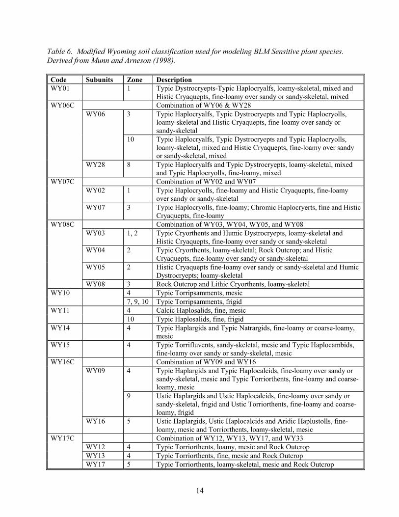
14

Table 6. Modified Wyoming soil classification used for modeling BLM Sensitive plant species. Derived from Munn and Arneson (1998). Code Subunits Zone Description WY01 1 Typic Dystrocryepts-Typic Haplocryalfs, loamy-skeletal, mixed and

Histic Cryaquepts, fine-loamy over sandy or sandy-skeletal, mixed Combination of WY06 & WY28

3 Typic Haplocryalfs, Typic Dystrocryepts and Typic Haplocryolls, loamy-skeletal and Histic Cryaquepts, fine-loamy over sandy or sandy-skeletal

WY06

10 Typic Haplocryalfs, Typic Dystrocryepts and Typic Haplocryolls, loamy-skeletal, mixed and Histic Cryaquepts, fine-loamy over sandy or sandy-skeletal, mixed

WY06C

WY28 8 Typic Haplocryalfs and Typic Dystrocryepts, loamy-skeletal, mixed and Typic Haplocryolls, fine-loamy, mixed

Combination of WY02 and WY07 WY02 1 Typic Haplocryolls, fine-loamy and Histic Cryaquepts, fine-loamy

over sandy or sandy-skeletal

WY07C

WY07 3 Typic Haplocryolls, fine-loamy; Chromic Haplocryerts, fine and Histic Cryaquepts, fine-loamy

Combination of WY03, WY04, WY05, and WY08 WY03 1, 2 Typic Cryorthents and Humic Dystrocryepts, loamy-skeletal and

Histic Cryaquepts, fine-loamy over sandy or sandy-skeletal WY04 2 Typic Cryorthents, loamy-skeletal; Rock Outcrop; and Histic

Cryaquepts, fine-loamy over sandy or sandy-skeletal WY05 2 Histic Cryaquepts fine-loamy over sandy or sandy-skeletal and Humic

Dystrocryepts; loamy-skeletal

WY08C

WY08 3 Rock Outcrop and Lithic Cryorthents, loamy-skeletal 4 Typic Torripsamments, mesic WY10 7, 9, 10 Typic Torripsamments, frigid 4 Calcic Haplosalids, fine, mesic WY11 10 Typic Haplosalids, fine, frigid

WY14 4 Typic Haplargids and Typic Natrargids, fine-loamy or coarse-loamy, mesic

WY15 4 Typic Torrifluvents, sandy-skeletal, mesic and Typic Haplocambids, fine-loamy over sandy or sandy-skeletal, mesic

Combination of WY09 and WY16 4 Typic Haplargids and Typic Haplocalcids, fine-loamy over sandy or

sandy-skeletal, mesic and Typic Torriorthents, fine-loamy and coarse-loamy, mesic

WY09

9 Ustic Haplargids and Ustic Haplocalcids, fine-loamy over sandy or sandy-skeletal, frigid and Ustic Torriorthents, fine-loamy and coarse-loamy, frigid

WY16C

WY16 5 Ustic Haplargids, Ustic Haplocalcids and Aridic Haplustolls, fine-loamy, mesic and Torriorthents, loamy-skeletal, mesic

Combination of WY12, WY13, WY17, and WY33 WY12 4 Typic Torriorthents, loamy, mesic and Rock Outcrop WY13 4 Typic Torriorthents, fine, mesic and Rock Outcrop

WY17C

WY17 5 Typic Torriorthents, loamy-skeletal, mesic and Rock Outcrop

15

10 Rock Outcrop and Typic Torriorthents, loamy-skeletal, mixed, frigid WY33 9 Lithic Torriorthents, loamy-skeletal, frigid and Rock Outcrop

WY18 5 Typic Torriorthents and Entic Haplistolls, fine-loamy, mesic WY19 5 Typic Haplogypsids, fine, mesic WY20 6 Typic Hapludalfs and Typic Argiudolls, fine-loamy and Typic

Haplaquolls, fine, frigid WY22 6 Typic Argiudolls and Typic Haplaquolls, fine-loamy, frigid WY23 7 Typic Argiustolls, fine-loamy and Typic Argiustolls fine-loamy over

sandy or sandy-skeletal, mixed, frigid WY25 7 Ustic Torriorthents and Aridic Ustochrepts, loamy-skeletal, frigid WY27 7 Typic Torrifluvents and Typic Haplaquolls, fine-loamy over sandy or

sandy-skeletal, mixed, frigid WY29 8 Histic Cryaquepts and Typic Cryaquolls, fine-loamy over sandy or

sandy-skeletal, mixed Combination of WY30, WY31, and WY32 WY30 8 Typic Dystrocryepts and Lithic Cryorthents, loamy-skeletal, mixed

and Rock Outcrop WY31 8 Typic Dystrocryepts and Typic Cryorthents, loamy-skeletal, mixed

WY31C

WY32 8 Typic Dystrocryepts, loamy-skeletal, mixed and Rock Outcrop WY34 9 Ustic Haplargids and Ustic Natrargids, fine-loamy, frigid WY35 9 Typic Natrargids and Typic Torriorthents, fine, frigid WY36 9 Ustic Torriorthents and Ustic Haplocalcids, coarse-loamy, frigid WY37 9 Typic Petrocalcids and Ustic Calciargids, fine-loamy over sandy or

sandy-skeletal, frigid Combination of WY38, WY39, and WY43 WY38 9 Ustic Haplocambids and Ustic Haplargids, coarse-loamy, frigid WY39 10 Ustic Haplargids, Ustic Haplocambids and Ustic Natrargids, fine-

loamy, mixed, frigid

WY38C

WY43 6 Ustic Haplargids and Ustic Haplocambids fine and fine-loamy, mesic Combination of WY21, WY24, WY26, and WY40 WY21 6 Ustic Haplocambids and Ustic Torriorthents, fine, frigid and Rock

Outcrop WY24 7 Ustic Haplocambids and Ustic Torriorthents, fine, frigid WY26 7 Ustic Torriorthents and Ustic Haplocambids, fine, frigid

WY40C

WY40 10 Ustic Haplocambids and Ustic Torriorthents, coarse-loamy, mixed and Typic Torrifluvents, loamy-skeletal, mixed, frigid

WY41 10 Aridic Haplustolls and Ustic Haplocambids, fine-loamy, frigid

WY42 3, 5 Typic Hapludolls and Typic Hapludalfs, loamy-skeletal, mixed, frigid 7 Ustic Haplargids and Ustic Torrifluvents, fine-loamy over sandy or

sandy-skeletal, mixed, mesic WY44

9 Ustic Haplargids and Typic Torrifluvents, fine-loamy over sandy or sandy-skeletal, mixed, mesic

WY45 8 Typic Hapludalfs and Aridic Haplustepts, loamy-skeletal, mixed, frigid

16

Table 7. Modified Gap land cover classification for Wyoming derived from Merrill et al. (1996), and Driese et al. (1997). Note: The primary cover types of clearcut conifer (42007) and burned conifer (42016) were replaced by their secondary types for this analysis.

Code Landcover Category Wyoming Units AcDun Active sand dunes 73001 AlpRk Alpine bare rock and soil 74002, 91001 AlpTn Alpine tundra 82001 Aspen Aspen forest 41001 BkSge Black sagebrush steppe 32008 BrOak Bur oak woodland 41002 BsnRk Basin bare rock and soil 74001 DougF Douglas-fir forest 42003 DstSh Desert shrub 32010 FrRip Forest-dominated riparian 61001 GrsWd Greasewood fans and flats 32012 GrWet Graminoid-dominated wetland 62002, 62003 Hmdis Human disturbed 11001, 21001, 21002, 75001 Junpr Juniper woodland 42015 Limbr Limber pine woodland and scrub 42009 LodgP Lodgepole pine forest 42004 MesSh Mesic upland shrub grassland 31003, 32001 MGras Mixed grass prairie 31001 MtSge Mountain big sagebrush 32005, 32006 Pdosa Ponderosa pine forest 42010 Playa Unvegetated playa 71001 SbAlp Subalpine meadow 82002 SGras Short grass prairie 31002 ShRip Shrub-dominated riparian 62001 SpFir Spruce-fir forest 42001 StBsh Saltbush fans and flats 32011 VgDun Vegetated dunes 32013 Water Open water 52001 WhtBk Whitebark pine forest 42008 WySge Wyoming big sagebrush 32007, 32009 XerSh Xeric upland shrub 32002

17

Table 8. Biomes used for selecting absent locations for validation of plant models. Modified from Barbour and Billings (2000).

Code Biome ALP Alpine EDF Eastern deciduous forest FOOT Foothills (transition between RMF and Great Plains grasslands/

Intermountain desert steppe) IDGRS Intermountain desert steppe/Great Plains grasslands IDS Intermountain desert steppe RMF Rocky Mountain forest WET Wetlands

and sufficient distance between points. These initial 1200 points were checked for accuracy by comparing location and elevation data from the original specimen labels with 1:100,000 DRGs in ArcView and repositioned as necessary. Over 100 points were dropped from the repositioned point set based on a reduced distance criterion of 5200 m, along with points whose TRS values (as obtained from the public land survey system), did not match the values in the corresponding herbarium records. Two more rounds of random selection occurred, each emphasizing proportional representation of the remaining variables (Table 2) that were under-sampled in the earlier rounds. Ultimately we identified a subset of 1206 potential absent points for modeling that adequately represented the range of environmental predictors and provided good spatial representation across the state. For each target species, the pool of potential absence sites was further reduced depending on whether the plant was actually known from any of the absent points. Additional points were eliminated if they were from the same TRS section or within 2400 meters of a known present point for that species. Finally, absent points were removed if they were from a biome type in which the species was not likely to occur (Table 8). This helped reduce possible inflation of classification success due to use of locations that were obviously unsuitable, the so-called problem of the "naughty-nots" (Michael Austin, personal communication in Fertig et al. 2002). Once presence and absence locations were identified for each target species, we randomly subdivided each group of points into model-building and validation data sets. For species with less than 16 present locations, no points were selected for validation and model testing was conducted only with absent points. If a species was known from 16 or more locations, we used 25% of the total number of present locations for validation. After the number of desired validation points was calculated, we randomly stratified the available points by geographic area to minimize over-sampling present sites from the same general location. Absence points were also stratified by location, with 20% being randomly selected for validation and 80% for model construction. The final point sets for model-building and validation for our model of Cirsium aridum Dorn (Cedar Rim thistle) are shown in Figures 1 and 2.

Figure 1. Known present points for Cirsium aridum used for model-building and validation. Figure 2. Inferred

18

absence points for Cirsium aridum used for model-building and validation.

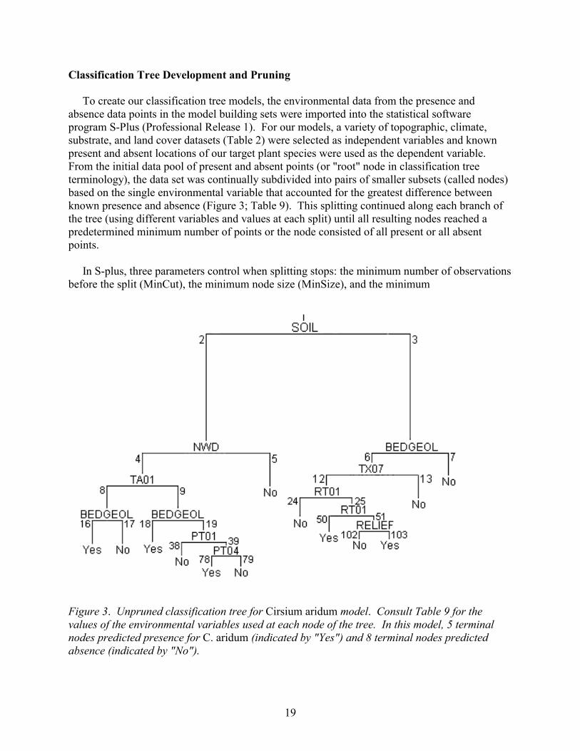
Classification Tree Development and Pruning To create our classification tree models, the environmental data from the presence and absence data points in the model building sets were imported into the statistical software program S-Plus (Professional Release 1). For our models, a variety of topographic, climate, substrate, and land cover datasets (Table 2) were selected as independent variables and known present and absent locations of our target plant species were used as the dependent variable. From the initial data pool of present and absent points (or "root" node in classification tree terminology), the data set was continually subdivided into pairs of smaller subsets (called nodes) based on the single environmental variable that accounted for the greatest difference between known presence and absence (Figure 3; Table 9). This splitting continued along each branch of the tree (using different variables and values at each split) until all resulting nodes reached a predetermined minimum number of points or the node consisted of all present or all absent points. In S-plus, three parameters control when splitting stops: the minimum number of observations before the split (MinCut), the minimum node size (MinSize), and the minimum Fvna

19

igure 3. Unpruned classification tree for Cirsium aridum model. Consult Table 9 for the alues of the environmental variables used at each node of the tree. In this model, 5 terminal odes predicted presence for C. aridum (indicated by "Yes") and 8 terminal nodes predicted bsence (indicated by "No").

20

Table 9. Classification tree node definitions for unpruned model of Cirsium aridum (MinPct = 0.0). Codes: Node_Num = node number; Node_Def = environmental variable selected at each node and the defining condition; Node_Size = total number of location points at each node; (Num_No,Num_Yes) = the number of absent and present points at each node; (Pct_No,Pct_Yes) = percentage of absent and present points at each node relative to the total number of absent and present points used to construct the model; Node_Type = presence (Yes) or absence (No) score assigned to the node based on the previous percentages. Terminal nodes are indicated by a * and terminal Yes nodes are in bold. Consult Figure 3 for a visual depiction of this classification tree and tables 2, 4, 5, 6, and 7 for values of the environmental variables. Note: The node definitions in this example are identical to those used in model b in Figure 4 (MinPct = 0.2) except for the elimination of nodes 16 and 17 and node 8 being classified as a terminal Yes node.

Node_Num) Node_Def Node_Size (Num_No,Num_Yes) (Pct_No,Pct_Yes) Node_Type 1) root 976 (961,15) (100,100) Yes 2) SOIL:WY34,WY41 67 (55,12) (5.7,80) Yes 4) NWD<58.5 40 (28,12) (2.9,80) Yes 8) TA01<-6.99 10 (2,8) (0.2,53.3) Yes 16) BEDGEOL:Eoe,Olg 8 (0,8) (0, 53.3) Yes * 17) BEDGEOL: Eol,TQc 2 (2,0) (0.2, 0) No * 9) TA01>-6.99 30 (26,4) (2.7,26.7) Yes 18) BEDGEOL:Eol 2 (0,2) (0,13.3) Yes * 19) BEDGEOL:Eoe,MiPl,Olg,Pal,TQc 28 (26,2) (2.7,13.3) Yes 38) PT01<1.29 21 (21,0) (2.2,0) No * 39) PT01>1.29 7 (5,2) (0.5,13.3) Yes 78) PT04<3.945 3 (1,2) (0.1,13.3) Yes * 79) PT04>3.945 4 (4,0) (0.4,0) No * 5) NWD>58.5 27 (27,0) (2.8,0) No * 3) SOIL:WY01,WY06C,WY07C,WY08C,WY10,WY11,WY14,WY15,WY16C,WY17C, WY18, WY20,WY23,WY27,WY31C,WY35,WY36,WY38C,WY40C,WY42,WY44,WY45 909 (906,3) (94.3,20) No 6) BEDGEOL:Eoe 179 (176,3) (18.3,20) Yes 12) TX07<25.83 37 (34,3) (3.5,20) Yes 24) RT01<7.415 26 (26,0) (2.7,0) No * 25) RT01>7.415 11 (8,3) (0.8,20) Yes 50) RT01<7.43 2 (0,2) (0,13.3) Yes * 51) RT01>7.43 9 (8,1) (0.8,6.7) Yes 102) RELIEF<244 7 (7,0) (0.7,0) No * 103) RELIEF>244 2 (1,1) (0.1,6.7) Yes * 13) TX07>25.83 142 (142,0) (14.8,0) No * 7) BEDGEOL:Eex,Ein,Eol,H2O,Kmix,Ksh,Kss,MiPl,Olg,PCf,PCm,PTJ,Pal,Pze,Qal,Qlc, Qls,Qs, Qt,Qvf,TQc,Tlvf 730 (730,0) (76,0) No *

21

node deviance (MinDev). Splitting continues until a node is homogeneous (node deviance = 0), or the number of observations in a node is less than the number of MinSize observations. When a split does occur, each node of the node pair must have at least the MinCut number of observations, thus MinSize is always at least two times larger than the value of MinCut. We found by experimentation that the optimal size for MinCut was 10% of the number of present points in the model building dataset. We found that if MinCut and MinSize were too small, the resulting models became overly complex (and validated poorly), while if these values were too high the models were too simplistic, obscuring potentially interesting environmental relationships (Fertig et al. 2002). We chose MinDev to be 0.01, the default value assigned by S-Plus. When a branch of the classification tree can no longer be subdivided it is called a leaf or terminal node. By default, S-Plus assigns a value of "yes" (predicted present) for terminal nodes in which the majority of points are from known populations of the target species, or "no" (predicted absent) if the majority of points are from absent locations. To compensate for the low number of present points available for the model relative to the number of absent points, we reclassified the terminal nodes based on the percentage of available present and absent points at the node. In our revised classification, terminal nodes were ranked "yes" if the percentage of all available present points at the node was greater than the percentage of all available absent points, or "no" if the percentage of all available absent points at the node was greater than the percentage of present points (Fertig et al. 2002). By making this change we significantly reduced the number of nodes with a high percentage (but minority) of present points that would have otherwise been scored as "no". This resulted in models that predicted more geographic area as potential habitat but had a significant reduction in omission error (false negatives) (Fertig et al. 2002). An example of a revised S-Plus classification tree for Cirsium aridum Dorn is shown in Figure 3 and Table 9. The model was generated using a MinCut of 2 and a MinSize of 4. Each line in the table contains the node number (Node_Num), the environmental variable selected by the model at that node (Node_Def), the total number of location points at that node (Node_Size), the number of absent and present points (Num_No, Num_Yes), the percentage of absent and present points at the node relative to the total number of available absent and present points in the model (Pct_No, Pct_Yes), and the presence (Yes) or absence (No) score assigned to the node based on the previous percentages (Node_Type). Node 1 (also called the root node) represents the entire model-building dataset. In this example, the model began with 976 location points, of which 961 were absent and 15 were present (with each representing 100% of the available absent or present points). The root node was subdivided into nodes 2 and 3 based on the modified Wyoming soil classification (SOIL). All location points with a state soil value of WY34 or WY41 (Table 6) were assigned to node 2, while all other points were placed in node 3*. In all, 67 records (55 absent and 12 present) were placed in node 2, while 909 points (906 absent and 3 present) went to node 3. The 67 points in node 2 were subdivided into two smaller subsets (nodes 4 and 5) based on the number of wet days (NWD). 40 points (28 absent and 12 present) with the number of wet days less than 58.5 were placed in node 4, while the remaining 27 points with NWD > 58.5 went *No location data for this model were from WY19, WY22, WY29, or WY37 soil types.

22

to node 5. Since node 5 contained only absent points, it was not further subdivided even though the number of points still exceeded the MinSize value of 4. Node 4, however, could still be split into two smaller groups (nodes 8 and 9) based on a threshold value of -6.99º C for average January air temperature. Splitting continued along all branches of this tree until every node contained only present or absent points (nodes 13, 16, 17, 18, 24, 38, 50, 79, 102) or the nodes contained fewer than 4 total points (based on the value of MinSize) or two or more points (based on the MinCut value of 2) as in nodes 78 and 103. The final step in developing a classification tree is to simplify the tree by removing extraneous branches by "pruning". Unpruned models tend to overfit the data used in model construction, resulting in predicted distribution maps that strongly match present points, but often perform poorly in predicting independent validation data. Although S-PLUS has pruning algorithms, they do not work with our revised classification scheme based on percentages. We developed a new pruning method that eliminated nodes in which the percentage of present or absent points were at or below a selected threshold called the minimum percent for pruning (MinPct). Using an ArcInfo AML, we could identify the MinPct thresholds at which successive terminal nodes could be pruned back towards the root node. Additional pruning was done for models in which a pair of terminal nodes at the same branch were both coded as either "yes" or "no". Such "companion nodes" were pruned back to the preceding node. Figure 4 illustrates the application of increasingly large MinPct values to the classification tree for Cirsium aridum. In general, we found that lower values of MinPct resulted in more complex models that predicted relatively small geographic areas and often had higher omission error rates for validation point sets. By contrast, higher MinPct cutoffs produced models that predicted significantly larger ranges and had low omission error, but often relatively high commission (false positive) error rates (Fertig et al. 2002). Creation of Potential Range Maps Completed classification trees typically consist of 1-6 branches culminating in a terminal "yes" node, each of which identifies different combinations of environmental variables and values that describe the potential habitat of the target species. Table 10 depicts the five distinct "yes" branches or node pathways for the Cirsium aridum model pruned with a MinPct of 0.2 (Figure 4b, Table 9). For example, node pathway "a" (nodes 8, 4, 2) indicates that C. aridum is predicted to occur in areas that have soil types WY34 or WY41, fewer than 58.5 wet days per year, and average January air temperature less than -6.99º C. Node pathway "b" (defined by nodes 18, 9, 4, 2) demonstrates that this species can also occur under the same conditions of soil and wet days if average January air temperature is greater than -6.99º C as long as bedrock geology consists of late Eocene deposits (Eol). Other potential "yes" pathways emphasize other combinations of environmental variables, including local relief, total January shortwave radiation, maximum July air temperature, and average April and January monthly precipitation. In GIS we created potential distribution maps by intersecting the selected environmental variables at each node of a "yes" path to identify just those geographic locations that met every condition specified in the path. The final map was produced by merging the areas selected in

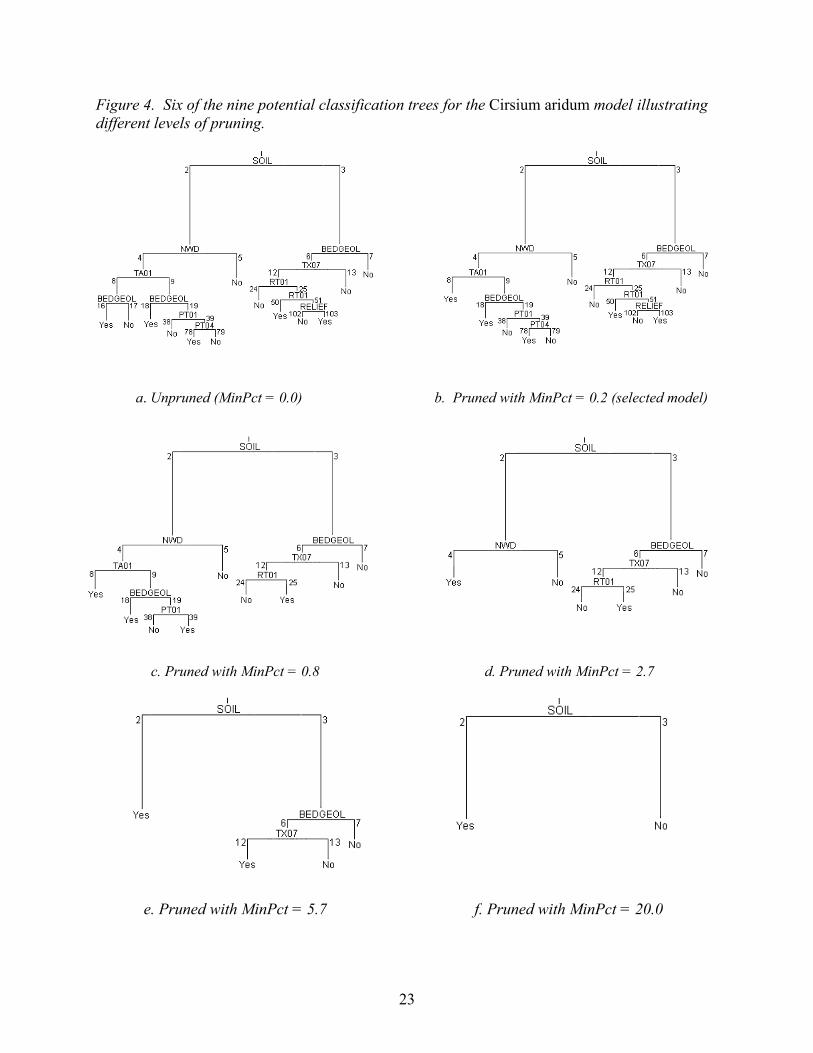
Figure 4. Six of the nine potential classification trees for the Cirsium aridum model illustrating different levels of pruning.

a. Unpruned (MinPct = 0.0) b. Pruned with MinPct = 0.2 (selected model) c. Pruned with MinPct = 0.8 d. Pruned with MinPct = 2.7

23

e. Pruned with MinPct = 5.7

f. Pruned with MinPct = 20.0

24

Table 10. Path composition and likelihood for classification tree model of Cirsium aridum. Yes Path Node List % of Present Points Likelihood Class

a 8, 4, 2 53.3 High b 18, 9, 4, 2 13.3 Medium c 78, 39, 19, 9, 4, 2 13.3 Medium d 50, 25, 12, 6, 3 13.3 Medium e 103, 51, 25, 12, 6, 3 6.7 Low

each separate pathway and overlaying the coverage on a state map with county boundaries and US and Interstate highways (Figure 5). Not all pathways that describe potential habitat for a species are equally probable. In the case of Cirsium aridum, path "a" contained 8 of the 15 known present points (53.3%) used to construct the model, while paths b, c, and d each contained 2 present points (13.3% each) and path e had just 1 present point (6.7%) (tables 9, 10). To help differentiate between the relative significance of each pathway, we developed a simple scoring system to measure the likelihood of any given modeled point belonging to a specific pathway. Pathways were scored as "high" if the percentage of present points for the path were at least twice the average value for all paths, "low" if the percentage of present points were less than one-half the average value, and "medium" if the percentage of present points were between one-half and twice the average for all paths (Table 10). In the final potential range map, each likelihood class was color-coded using a different gray tone to visually depict areas of differing probability of likely habitat (Figure 5). Model Validation and Selection Using automated pruning algorithms we were able to produce 2-13 different classification tree models for each of our target species. For those species with more than 16 known present points, we used validation with independent present and absent points to measure the accuracy of each classification tree in order to select the single model that best described the potential range of the species. Six different classification success parameters can be measured (Table 11). Total success rate is a measure of the percentage of all points (both present and absent) that are correctly classified by the model. This can be subdivided into the present success rate (the percentage of known present points classified correctly by the model) and absent success rate (the percentage of known absent points classified correctly). By contrast, total error rate is a calculation of the percentage of all points (present and absent) that are misclassified by the model and consists of two components: omission or false negative error rate (the percentage of known present points that are misclassified) and commission or false positive error rate (the percentage of known absent points that are misclassified by the model) (Franklin 1995; Fielding 2002). These classification success and error metrics can be applied to both model-building and validation data sets (Table 12). Since model-building data are used to construct the model their

25

Figure 5. Potential distribution of Cirsium aridum in Wyoming based on a classification tree model pruned with a MinPct of 0.2.

26

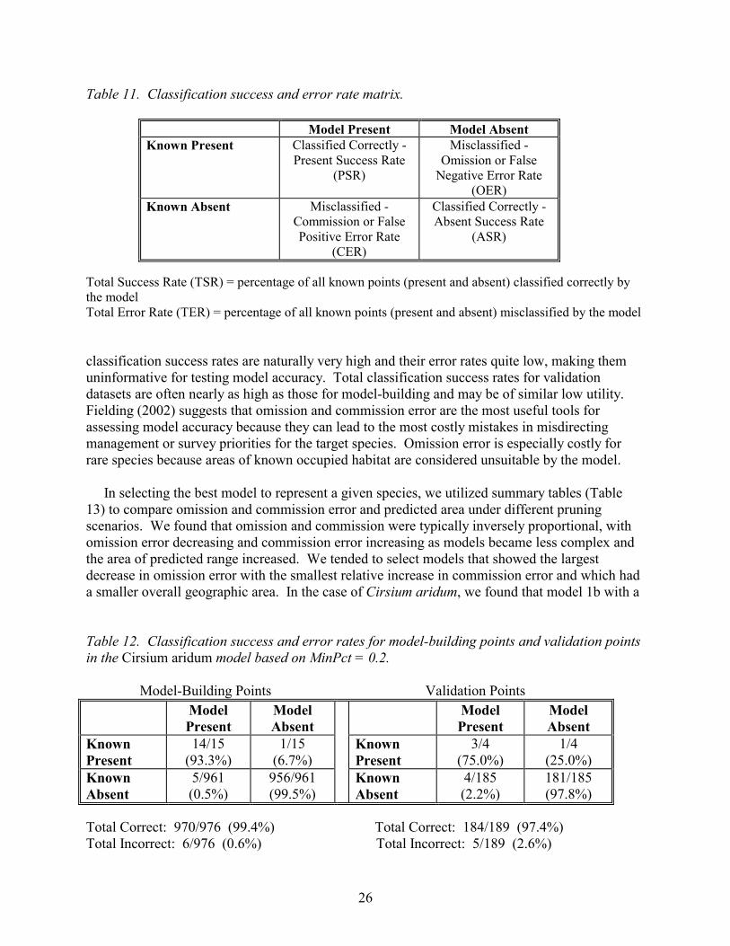
Table 11. Classification success and error rate matrix.

Model Present Model Absent Known Present Classified Correctly -

Present Success Rate (PSR)

Misclassified -Omission or False

Negative Error Rate (OER)

Known Absent Misclassified - Commission or False Positive Error Rate

(CER)

Classified Correctly - Absent Success Rate

(ASR)

Total Success Rate (TSR) = percentage of all known points (present and absent) classified correctly by the model Total Error Rate (TER) = percentage of all known points (present and absent) misclassified by the model classification success rates are naturally very high and their error rates quite low, making them uninformative for testing model accuracy. Total classification success rates for validation datasets are often nearly as high as those for model-building and may be of similar low utility. Fielding (2002) suggests that omission and commission error are the most useful tools for assessing model accuracy because they can lead to the most costly mistakes in misdirecting management or survey priorities for the target species. Omission error is especially costly for rare species because areas of known occupied habitat are considered unsuitable by the model. In selecting the best model to represent a given species, we utilized summary tables (Table 13) to compare omission and commission error and predicted area under different pruning scenarios. We found that omission and commission were typically inversely proportional, with omission error decreasing and commission error increasing as models became less complex and the area of predicted range increased. We tended to select models that showed the largest decrease in omission error with the smallest relative increase in commission error and which had a smaller overall geographic area. In the case of Cirsium aridum, we found that model 1b with a Table 12. Classification success and error rates for model-building points and validation points in the Cirsium aridum model based on MinPct = 0.2. Model-Building Points Validation Points Model

Present Model Absent

Model Present

Model Absent

Known Present

14/15 (93.3%)

1/15 (6.7%)

Known Present

3/4 (75.0%)

1/4 (25.0%)

Known Absent

5/961 (0.5%)

956/961 (99.5%)

Known Absent

4/185 (2.2%)

181/185 (97.8%)

Total Correct: 970/976 (99.4%) Total Correct: 184/189 (97.4%) Total Incorrect: 6/976 (0.6%) Total Incorrect: 5/189 (2.6%)

27

MinPct of 0.2% had the greatest drop in omission with the smallest increase in commission error, so we selected this model for the final report (Figure 5). Modeling Plants with Limited Data (Range/Intersection Models) Although classification tree analysis can be applied to datasets of any size, the technique is less useful when the number of available case studies drops below a minimum size threshold (Breiman et al. 1984). In this study, we found that classification trees developed with fewer than 8 present locations usually resulted in overly simple models with 3 or fewer terminal nodes. Due to their simplicity, these models often omitted potentially useful environmental information in tree construction and, in many cases, overestimated the area of likely potential habitat. For these situations we developed an alternative protocol (range/intersection modeling) that used the environmental conditions correlated with each present location in the model-building dataset to identify additional geographic areas in the state with the same environmental attributes (Fertig et al. 2002). Unlike classification tree models, range/intersection models did not use environmental information from absent locations for model development and were created entirely in GIS, rather than using statistical software. The final distribution maps produced by the range/ intersection method could be validated in the same way as classification tree models, although present points were usually not available for validation if fewer than 16 points existed for model building. The same environmental variables used in classification tree modeling were used to construct range/intersection models except for number of wet days, maximum July air temperature, number of frost days, and growing degree days. The values of categorical variables used in range/intersection modeling were calculated using the Field/Summarize function of ArcView (Table 14). In some instances expert knowledge was used to add or delete values if the selected Table 13. Summary of validation success and predicted area for 9 potential models of Cirsium aridum. Codes: MinPct = minimum percent threshold for pruning; OER = omission error rate, CER = commission error rate.

Model Points Validation Points

Model MinPct (%)

OER (%)

CER (%)

OER (%)

CER (%)

# Yes Paths

Predicted Area (km2)

% of WY

1a 0.0% 6.7 0.3 50.0 1.6 5 1,761.4 0.70 1b 0.2% 6.7 0.5 25.0 2.2 5 2,203.7 0.87 1c 0.5% 6.7 0.9 25.0 3.2 5 2,947.4 1.16 1d 0.8% 6.7 1.6 25.0 3.2 4 4,170.1 1.65 1e 2.7% 6.7 3.7 25.0 6.5 2 10,635.8 4.20 1f 3.5% 6.7 6.3 25.0 10.3 2 14,792.4 5.84 1g 5.7% 6.7 9.2 25.0 13.5 2 24,453.5 9.66 1h 18.3% 0.0 23.8 25.0 31.4 2 67,077.6 26.50 1i 20.0% 20.0 5.7 50.0 9.7 1 18,818.8 7.43

28

values were considered incomplete or erroneous. Minimum and maximum values of continuous variables were also determined using the Field/Statistics function, but to improve prediction accuracy these values were buffered using the following formulas: MinNew = Min - dVar and MaxNew = Max + dVar where dVar = K * Mean for ELEV, RELIEF, PT, and RT variables and dVar = 1 ºC * (K/0.05) for TA variables. Values of K ranged from 0.05 to 0.2 depending on whether we wished to Table 14. Values of variables used in construction of range/intersection model of Trifolium barnebyi in Wyoming with K = 0.05.

Continuous Variables Variable Units Min

Max Mean dVar MinNew MaxNew

Elevation m 1747 2029 1904 95 1652 2124 Relief m 96 220 155 8 88 228 Total January Precipitation

cm

2.09 2.56 2.26 0.11 1.98 2.67

Total April Precipitation

cm

3.89 4.70 4.30 0.22 3.67 4.92

Total July Precipitation

cm

1.70 2.15 1.89 0.09 1.61 2.24

Total October Precipitation

cm

2.65 3.07 2.82 0.14 2.51 3.21

Average January Air Temperature

ºC - 7.39 - 6.84 - 7.09 1 - 8.39 - 5.84

Average April Air Temperature

ºC 4.15 6.24 5.34 ºC 1 3.15 7.24

Average July Air Temperature

ºC 18.01 20.21 19.25 ºC 1 17.01 21.21

Average October Air Temperature

ºC 5.57 7.06 6.41 ºC 1 4.57 8.06

Total January Shortwave Radiation

MJ/m2/day 6.82 7.11 6.99 0.35 6.47 7.46

Total July Shortwave Radiation

MJ/m2/day 25.00 25.12 25.07 1.25 23.75 26.37

Categorical Variables

Variable Values Land Cover Junpr Bedrock Geology Ksh, PTJ WY Soil WY16C, WY35 Surface Geology Ri, sci

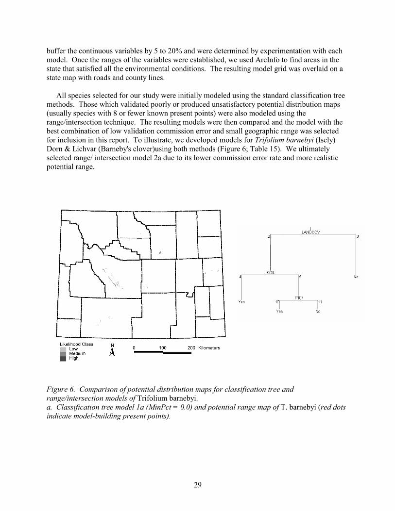
buffer the continuous variables by 5 to 20% and were determined by experimentation with each model. Once the ranges of the variables were established, we used ArcInfo to find areas in the state that satisfied all the environmental conditions. The resulting model grid was overlaid on a state map with roads and county lines. All species selected for our study were initially modeled using the standard classification tree methods. Those which validated poorly or produced unsatisfactory potential distribution maps (usually species with 8 or fewer known present points) were also modeled using the range/intersection technique. The resulting models were then compared and the model with the best combination of low validation commission error and small geographic range was selected for inclusion in this report. To illustrate, we developed models for Trifolium barnebyi (Isely) Dorn & Lichvar (Barneby's clover)using both methods (Figure 6; Table 15). We ultimately selected range/ intersection model 2a due to its lower commission error rate and more realistic potential range.

29

Figure 6. Comparison of potential distribution maps for crange/intersection models of Trifolium barnebyi. a. Classification tree model 1a (MinPct = 0.0) and potentiindicate model-building present points).

lassification tree and

al range map of T. barnebyi (red dots

30

Figure 6. Continued. b. Classification tree model 1b (MinPct = 3.4) and potentia c. Range/Intersection model 2a and potential range map of T

l range map of T. barnebyi.

. barnebyi.

31

Table 15. Comparison of validation success rates for classification tree and range/intersection models of Trifolium barnebyi. Model Points Validation Points

Model MinPct OER (%) CER (%) OER (%) CER (%) Predicted

Area (Km2)

% of WY

1a 0.0 0 0 na 3.6 300.4 0.12 1b 3.4 0 3.4 na 14.3 5719.6 2.26 2a na 0 0 na 0 74.8 0.03

Modeling Wetland Plants Modeling wetland plants presents a special challenge because there is no statewide dataset of wetland features, which are typically very fine-grained and often not represented on maps of large spatial extents, such as the state of Wyoming. If such a dataset did exist, there would still be the problem of the positional errors associated with the wetland features and the point datasets. These spatial inaccuracies can result in incorrect wetland attributes being assigned to present and absent location points for our modeled species, which in turn can propagate errors in classification tree and range/intersection models. Our approach to the problem of modeling wetland plants was to first create a standard classification tree or range/intersection model, as if the plant species was an upland plant. Since these models predict a lot of upland area and tend to greatly overestimate the potential area and habitats available to wetland plants, we then intersected the upland models with a riparian model to get a more realistic estimate of potential area (Fertig et al. 2002). We created the riparian/aquatic model from the 1:100,000 enhanced hydrography digital line graphs (DLGs) for Wyoming available from the Wyoming Natural Resources Data Clearinghouse (http://www.sdvc.uwyo.edu/clearinghouse/). This dataset includes both perennial and intermittent lakes, ponds, reservoirs, rivers, streams, marshlands, and ephemeral washes (Table 16). Riparian areas were modeled by buffering the hydrographic features using buffer widths determined by the Wyoming Gap Analysis Project (Merrill et al. 1996) (Table 17). The buffer areas were attributed to indicate the source hydrographic feature and whether the feature was perennial or intermittent. This allowed us to use only those riparian types in which a plant species occurred when intersecting the riparian model with the upland model and was an improvement over the riparian/aquatic model used in our earlier wetland plant modeling efforts (Fertig et al. 2002), which indicated only presence or absence of perennial features. The earlier model also had a problem in that the large lakes and reservoirs had been digitized from satellite imagery and were significantly different from the corresponding features in the enhanced hydrography DLGs. We also repositioned the present points for our wetland species (usually by less than 100 m) to ensure they were near hydrographic features as represented by the 1:100,000 scale DRGs or hydrography DLGs. This helped ensure that the points received the correct riparian attribute value from the narrowed riparian features. The riparian types in which the present points occured were then determined from this attribute and only those types were intersected with the upland model.

32

Table 16. Riparian and aquatic habitat types used to intersect classification tree and range/intersection models for selected wetland obligate plant species.

Code Description LakI Lake or pond, intermittent LakP Lake or pond, perennial LakRipI Lake or pond riparian, intermittent LakRipP Lake or pond riparian, perennial ResI Reservoir, intermittent ResP Reservoir, perennial ResRipI Reservoir riparian, intermittent ResRipP Reservoir riparian, perennial StrRipI Stream riparian, intermittent StrRipP Stream riparian, perennial Wet Marsh or wetland WRiv Wide river WRivRip Wide river riparian Wsh Ephemeral wash

Table 17. Buffer widths applied to the hydrographic features used in the creation of the riparian/aquatic model.

Feature Strahler Stream Order

Buffer Width (m)

1 40 2 40 3 60 4 90 5 120 6 150

Stream

7 210 Reservoir 90 Lake or Pond 90 Wide River 300 Marsh or Wetland 0 Ephemeral Wash 0

Classification success and error rates were determined for both the upland model and the wetland model created from the intersection process. Due to the intersection, the omission error rates for the wetland model can be no lower than those for the upland model, but since the wetland model predicts significantly less area, the commission error rate was greatly reduced. The map for a wetland species shows the modeled riparian areas within the area predicted by the upland model, along with highways and county boundaries (Figure 7). Fpsa

33

igure 7. Potential distribution of Sisyrinchium pallidum in southeastern Wyoming. Light gray olygons represent areas of potential habitat for this species in upland areas, as derived from a tandard classification tree model. Darker gray lines superimposed over the light gray polygons re wetland habitats identified by our riparian model.

34

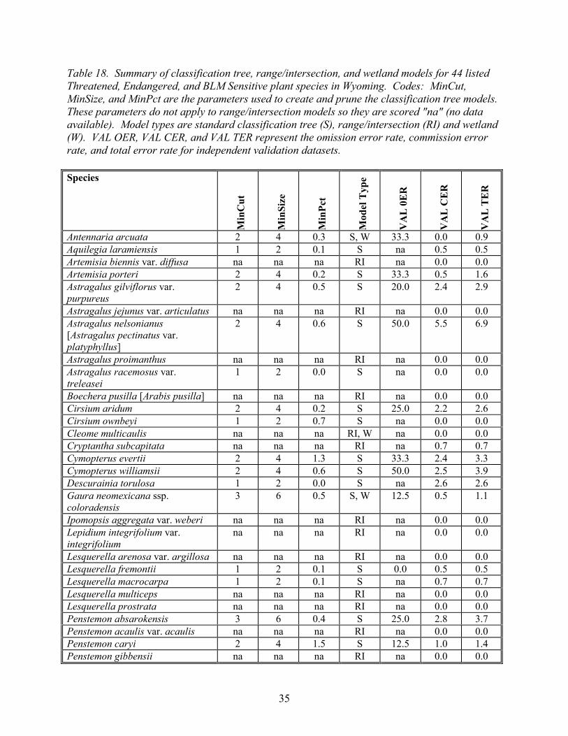
RESULTS AND DISCUSSION Summary of Potential Distribution Models Appendices A and B contain the final results of our modeling efforts for 44 listed Threatened, Endangered, and BLM Sensitive plants in Wyoming. The parameters and variables used to construct these models, as well as the classification success and error rates for validation data, are summarized in Tables 18-20. Of our 44 target species, 23 were modeled using standard classification tree analysis and 21 were developed with the range/intersection method. Six of these species were further modeled using the wetland protocol (4 derived from classification tree and 2 from range/intersection models). Twenty continuous and categorical environmental variables were used to construct our classification tree models, while only 16 of these variables were used for our range/intersection models (Tables 19-21). For the classification tree models, all but one variable (growing degree days) were selected by at least one model. Bedrock geology was the variable used most frequently, appearing in 38 of 44 models (86.4%) and being selected as the first variable in 6 of 23 classification tree models (26%). Among the most commonly used bedrock types were Eocene volcanic, Eocene lake sediment, Early Paleozoic calcareous sediment, and Quaternary landslide deposits. Soil variables were used in 35 models (79.5%) and were also selected first in 6 classification tree models (26%). The most frequently selected soil types represented aridic or poorly weathered inceptisols or entisols. At least one of the four total monthly precipitation variables was used in 39 models (88.6%), although no single precipitation variable occurred in more than 68% of the models. Likewise, the 5 temperature variables appeared in 32 models (72.7%), but only average January air temperature was used at least 30 times (68%). The only other variables used in over 70% of the models were relief (75%) and Gap land cover (72.7%) (Table 21). Number of wet days appeared in 10 of 23 classification tree models (making it the fifth most commonly used variable), but appears less significant overall because it was not used in range/intersection models. Results from independent validation suggest that our models do a very good job of identifying areas where rare species are unlikely to occur, but are less successful in correctly predicting known location points (Table 18). Commission error rates (false negatives) ranged from 0-5.5% (mean = 0.78%) for our validation data, indicating that very few of the known absent points for our target species were misclassified as being in suitable habitat. By contrast, omission error (false positives) was much higher, averaging 34.4% for the 18 species in which sufficient numbers of present points were available for validation. Our previous modeling work on a broad cross section of the state's flora, however, has demonstrated that omission error rates tend to decrease as the number of available present points for model construction increases (Fertig et al. 2002). Thus validation based on a limited number of independent data points derived from herbarium or natural heritage program records may be far less useful for testing model accuracy than actual on-the-ground field surveys. Overall, our models were extremely conservative in the amount of area predicted for the state's listed Threatened, Endangered, and BLM Sensitive plants. Total predicted area ranged from a low of 1.5 km2 (0.0006% of Wyoming) for Cleome multicaulis (Many-stemmed spider-

35

Table 18. Summary of classification tree, range/intersection, and wetland models for 44 listed Threatened, Endangered, and BLM Sensitive plant species in Wyoming. Codes: MinCut, MinSize, and MinPct are the parameters used to create and prune the classification tree models. These parameters do not apply to range/intersection models so they are scored "na" (no data available). Model types are standard classification tree (S), range/intersection (RI) and wetland (W). VAL OER, VAL CER, and VAL TER represent the omission error rate, commission error rate, and total error rate for independent validation datasets. Species

M

inC

ut

Min

Size

Min

Pct

Mod

el T

ype

VA

L 0E

R

VA

L C

ER

VA

L TE

R

Antennaria arcuata 2 4 0.3 S, W 33.3 0.0 0.9 Aquilegia laramiensis 1 2 0.1 S na 0.5 0.5 Artemisia biennis var. diffusa na na na RI na 0.0 0.0 Artemisia porteri 2 4 0.2 S 33.3 0.5 1.6 Astragalus gilviflorus var. purpureus

2 4 0.5 S 20.0 2.4 2.9

Astragalus jejunus var. articulatus na na na RI na 0.0 0.0 Astragalus nelsonianus [Astragalus pectinatus var. platyphyllus]

2 4 0.6 S 50.0 5.5 6.9

Astragalus proimanthus na na na RI na 0.0 0.0 Astragalus racemosus var. treleasei

1 2 0.0 S na 0.0 0.0

Boechera pusilla [Arabis pusilla] na na na RI na 0.0 0.0 Cirsium aridum 2 4 0.2 S 25.0 2.2 2.6 Cirsium ownbeyi 1 2 0.7 S na 0.0 0.0 Cleome multicaulis na na na RI, W na 0.0 0.0 Cryptantha subcapitata na na na RI na 0.7 0.7 Cymopterus evertii 2 4 1.3 S 33.3 2.4 3.3 Cymopterus williamsii 2 4 0.6 S 50.0 2.5 3.9 Descurainia torulosa 1 2 0.0 S na 2.6 2.6 Gaura neomexicana ssp. coloradensis

3 6 0.5 S, W 12.5 0.5 1.1

Ipomopsis aggregata var. weberi na na na RI na 0.0 0.0 Lepidium integrifolium var. integrifolium

na na na RI na 0.0 0.0

Lesquerella arenosa var. argillosa na na na RI na 0.0 0.0 Lesquerella fremontii 1 2 0.1 S 0.0 0.5 0.5 Lesquerella macrocarpa 1 2 0.1 S na 0.7 0.7 Lesquerella multiceps na na na RI na 0.0 0.0 Lesquerella prostrata na na na RI na 0.0 0.0 Penstemon absarokensis 3 6 0.4 S 25.0 2.8 3.7 Penstemon acaulis var. acaulis na na na RI na 0.0 0.0 Penstemon caryi 2 4 1.5 S 12.5 1.0 1.4 Penstemon gibbensii na na na RI na 0.0 0.0

36

flower) to nearly 8,500 km2 (3.3% of Wyoming) for Astragalus nelsonianus (Nelson's milkvetch) (Appendix A). The average predicted range of our 44 target species is 1590 km2, or about 0.06% of the state's total area. Application of Models and Caveats Correlational modeling can be a useful tool to describe the environmental conditions and habitats associated with rare plant species. In GIS, these habitat relationships can be used to generate potential range maps that indicate where a given species is likely to occur (and not occur). Accurate distribution maps and ecological descriptions can help land managers, consultants, and conservation biologists more efficiently select and prioritize areas for survey or reintroduction of rare plants, or identify areas where resource development will not interfere with the continued survival of these species (Elith and Burgman 2002; Fertig et al. 2002). Plant modeling also has great potential for conducting gap analyses to identify suites of species, habitats, or geographic areas that are under-represented in the existing network of special management areas across the state (Fertig and Thurston 2001). Finally, modeling can identify interesting patterns in the potential distribution and niche partitioning among closely related species, helping plant geographers generate hypotheses on the evolution of endemic and rare species (Fertig et al. 2002).

Species

M

inC

ut

Min

Size

Min

Pct

Mod

el T

ype

VA

L 0E

R

VA

L C

ER

VA

L TE

R

Penstemon haydenii na na na RI na 0.0 0.0 Phlox pungens 3 6 0.6 S 20.0 0.6 1.6 Physaria condensata 2 4 0.8 S 20.0 0.6 1.1 Physaria dornii na na na RI na 0.0 0.0 Physaria saximontana var. saximontana

3 6 0.6 S 50.0 2.4 4.0

Rorippa calycina 4 8 1.0 S, W 25.0 2.0 3.3 Shoshonea pulvinata 1 2 0.1 S 50.0 0.5 1.4 Sisyrinchium pallidum 2 4 0.5 S, W 100 0.6 3.6 Sphaeromeria simplex 2 4 0.2 S 60.0 2.2 3.8 Spiranthes diluvialis na na na RI, W na 0.7 0.7 Thelesperma caespitosum na na na RI na 0.0 0.0 Thelesperma pubescens na na na RI na 0.0 0.0 Townsendia microcephala na na na RI na 0.0 0.0 Trifolium barnebyi na na na RI na 0.0 0.0 Yermo xanthocephalus na na na RI na 0.0 0.0

37

Table 19. Summary of continuous environmental variables used in classification tree, range/intersection, and wetland models for 44 listed Threatened, Endangered, and BLM Sensitive plant species in Wyoming. Codes: Model types are standard classification tree (S), range/intersection (RI), and wetland (W). Elev = elevation, Relief = local relief, PT01 = total January precipitation, PT04 = total April precipitation, PT07 = total July precipitation, PT10 = total October precipitation, NWD = number of wet days, RT01 = total January shortwave radiation, RT07 = total July shortwave radiation TA01 = average January air temperature, TA04 = average April air temperature, TA07 = average July air temperature, TA10 = average October air temperature, NFD = number of frost days, and GDD = growing degree days. "x" in these columns indicates the variable was used in development of a classification tree model. "1" indicates the variable was chosen at the root node. "r" indicates a variable used in range/intersection models. Species

Mod

el T

ype

Elev

Rel

ief

PT01

PT04

PT07

PT10

NW

D

RT0

1

RT0

7

TA01

TA04

TA07

TA10

TX07

NFD

GD

D

Antennaria arcuata S,W x x 1 Aquilegia laramiensis S x x x Artemisia biennis var. diffusa

RI r r r r r r r r r r r r

Artemisia porteri S x x x 1 Astragalus gilviflorus var. purpureus

S x x 1

Astragalus jejunus var. articulatus

RI r r r r r r r r r r r r

Astragalus nelsonianus [Astragalus pectinatus var. platyphyllus]

S x 1 x x x

Astragalus proimanthus RI r r r r r r r r r r r r Astragalus racemosus var. treleasei

S x x x 1

Boechera pusilla [Arabis pusilla]

RI r r r r r r r r r r r r

Cirsium aridum S x x x x x x x Cirsium ownbeyi S x 1 x Cleome multicaulis RI, W r r r r r r r r r r r r Cryptantha subcapitata RI r r r r r r r r r r r r Cymopterus evertii S x x x Cymopterus williamsii S x x Descurainia torulosa S x x x x x x Gaura neomexicana ssp. coloradensis

S, W x 1 x

Ipomopsis aggregata var. weberi

RI r r r r r r r r r r r r

38

Species

Mod

el T

ype

Elev

Rel

ief

PT01

PT04

PT07

PT10

NW

D

RT0

1

RT0

7

TA01

TA04

TA07

TA10

TX07

NFD

GD

D

Lepidium integrifolium var. integrifolium

RI r r r r r r r r r r r r

Lesquerella arenosa var. argillosa

RI r r r r r r r r r r r r

Lesquerella fremontii S x x x Lesquerella macrocarpa S x x x 1 Lesquerella multiceps RI r r r r r r r r r r r r Lesquerella prostrata RI r r r r r r r r r r r r Penstemon absarokensis S x x x x Penstemon acaulis var. acaulis

RI r r r r r r r r r r r r

Penstemon caryi S x x x x Penstemon gibbensii RI r r r r r r r r r r r r Penstemon haydenii RI r r r r r r r r r r r r Phlox pungens S x x x x 1 x Physaria condensata S x x x Physaria dornii RI r r r r r r r r r r r r Physaria saximontana var. saximontana

S x x x x x

Rorippa calycina S, W x 1 x x x Shoshonea pulvinata S x x Sisyrinchium pallidum S, W x x x Sphaeromeria simplex S x x x Spiranthes diluvialis RI, W r r r r r r r r r r r r Thelesperma caespitosum

RI r r r r r r r r r r r r

Thelesperma pubescens RI r r r r r r r r r r r r Townsendia microcephala

RI r r r r r r r r r r r r

Trifolium barnebyi RI r r r r r r r r r r r r Yermo xanthocephalus RI r r r r r r r r r r r r

39

Table 20. Summary of categorical environmental variables used in classification tree, range/intersection, and wetland models for 44 listed Threatened, Endangered, and BLM Sensitive plant species in Wyoming. Codes: Model types are standard classification tree (S), range/intersection (RI), and wetland (W). Bedgeol = bedrock geology, Surfgeol = surficial geology, Soil = Wyoming soil classification, and Landcov = Gap land cover. "x" in these columns indicates the variable was used in development of a classification tree model. "1" indicates the variable was chosen at the root node. "r" indicates a variable used in range/intersection models. Species

Mod

el T

ype

Bed

geol

Sur

fgeo

l

Soi

l

Lan

dcov

Antennaria arcuata S, W x Aquilegia laramiensis S 1 Artemisia biennis var. diffusa RI r r r r Artemisia porteri S x x x Astragalus gilviflorus var. purpureus S x x Astragalus jejunus var. articulatus RI r r r r Astragalus nelsonianus [Astragalus pectinatus var. platyphyllus]

S x x x

Astragalus proimanthus RI r r r r Astragalus racemosus var. treleasei S x Boechera pusilla [Arabis pusilla] RI r r r r Cirsium aridum S x 1 Cirsium ownbeyi S x Cleome multicaulis RI, W r r r r Cryptantha subcapitata RI r r r r Cymopterus evertii S 1 x Cymopterus williamsii S 1 x x Descurainia torulosa S 1 x Gaura neomexicana ssp. coloradensis S, W x Ipomopsis aggregata var. weberi RI r r r r Lepidium integrifolium var. integrifolium RI r r r r Lesquerella arenosa var. argillosa RI r r r r Lesquerella fremontii S x 1 Lesquerella macrocarpa S x Lesquerella multiceps RI r r r r Lesquerella prostrata RI r r r r Penstemon absarokensis S 1 x x Penstemon acaulis var. acaulis RI r r r r Penstemon caryi S 1 x x Penstemon gibbensii RI r r r r Penstemon haydenii RI r r r r Phlox pungens S x x Physaria condensata S 1

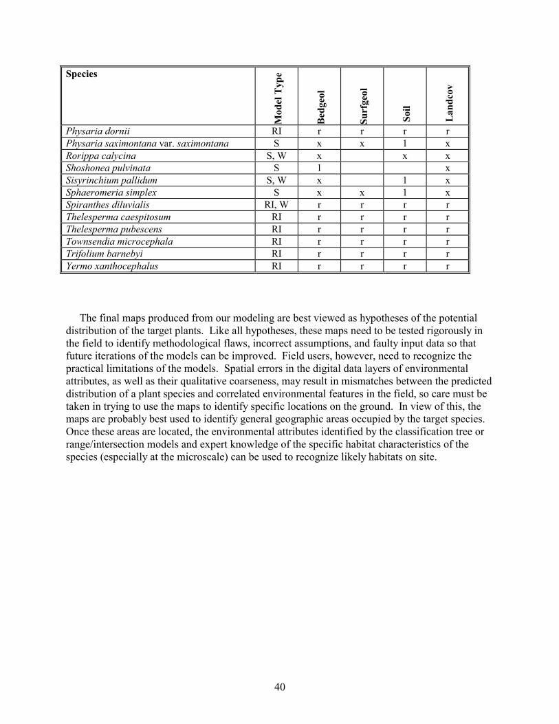
40

Species

Mod

el T

ype

Bedg

eol

Surf

geol

Soi

l

Lan

dcov

Physaria dornii RI r r r r Physaria saximontana var. saximontana S x x 1 x Rorippa calycina S, W x x x Shoshonea pulvinata S 1 x Sisyrinchium pallidum S, W x 1 x Sphaeromeria simplex S x x 1 x Spiranthes diluvialis RI, W r r r r Thelesperma caespitosum RI r r r r Thelesperma pubescens RI r r r r Townsendia microcephala RI r r r r Trifolium barnebyi RI r r r r Yermo xanthocephalus RI r r r r The final maps produced from our modeling are best viewed as hypotheses of the potential distribution of the target plants. Like all hypotheses, these maps need to be tested rigorously in the field to identify methodological flaws, incorrect assumptions, and faulty input data so that future iterations of the models can be improved. Field users, however, need to recognize the practical limitations of the models. Spatial errors in the digital data layers of environmental attributes, as well as their qualitative coarseness, may result in mismatches between the predicted distribution of a plant species and correlated environmental features in the field, so care must be taken in trying to use the maps to identify specific locations on the ground. In view of this, the maps are probably best used to identify general geographic areas occupied by the target species. Once these areas are located, the environmental attributes identified by the classification tree or range/intersection models and expert knowledge of the specific habitat characteristics of the species (especially at the microscale) can be used to recognize likely habitats on site.

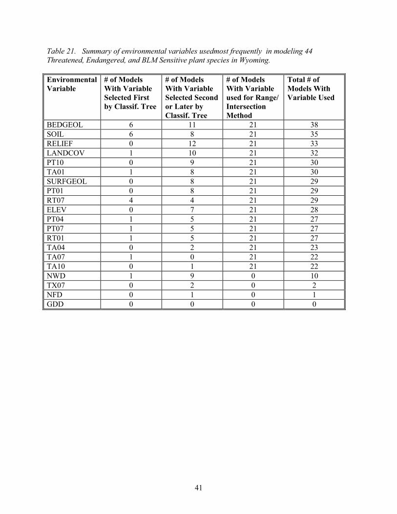
41

Table 21. Summary of environmental variables usedmost frequently in modeling 44 Threatened, Endangered, and BLM Sensitive plant species in Wyoming. Environmental Variable

# of Models With Variable Selected First by Classif. Tree

# of Models With Variable Selected Second or Later by Classif. Tree

# of Models With Variable used for Range/ Intersection Method

Total # of Models With Variable Used

BEDGEOL 6 11 21 38 SOIL 6 8 21 35 RELIEF 0 12 21 33 LANDCOV 1 10 21 32 PT10 0 9 21 30 TA01 1 8 21 30 SURFGEOL 0 8 21 29 PT01 0 8 21 29 RT07 4 4 21 29 ELEV 0 7 21 28 PT04 1 5 21 27 PT07 1 5 21 27 RT01 1 5 21 27 TA04 0 2 21 23 TA07 1 0 21 22 TA10 0 1 21 22 NWD 1 9 0 10 TX07 0 2 0 2 NFD 0 1 0 1 GDD 0 0 0 0

42

LITERATURE CITED American Association of Petroleum Geologists. 1967. Geological Highway Map of the Southern Rocky Mountain Region. Map # 2, United States Geological Highway Map Series. American Association of Petroleum Geologists, Tulsa, OK. Austin, M.P. 2002. Case studies of the use of environmental gradients in vegetation and fauna modeling: theory and practice in Australia and New Zealand. In: Predicting Species Occurrences: Issues of Accuracy and Scale, (Scott, J.M., P.J. Heglund, M.L. Morrison, J.B. Haufler, M.G. Raphael, W.A. Wall, F.B. Samson, eds.). Island Press, Covelo, CA. 483-489. Barbour, M.G. and W.D. Billings, eds. 2000. North American Terrestrial Vegetation, second edition. Cambridge University Press, NY. 708 pp.

Breiman, L., J.H. Friedman, R.A. Olshen, and C.J. Stone. 1984. Classification and Regression Trees. Chapman and Hall, NY. 358 pp.

Brown, J. H. and M.V. Lomolino. 1998. Biogeography. Sinauer Associates, Inc., Sunderland, MA. 691 pp.

Case, J.C., C.S. Arneson, and L.L. Hallberg. 1998. Preliminary 1:500,000-scale digital surficial geology map of Wyoming. Wyoming State Geological Survey, Geologic Hazards Section Digital Map 98-1 (HDSM 98-1).

Cornelisse, P. 2002. Announcing WY BLM Sensitive list update. Castilleja 21(3):8

Driese, K.L., W.A. Reiners, E.H. Merrill, and K.G. Gerow. 1997. A digital land cover map of Wyoming, USA: a tool for vegetation analysis. Journal of Vegetation Science 8:133-146.

Elith, J. and M. Burgman. 2002. Predictions and their validation: rare plants in the Central Highlands, Victoria, Australia. In: Predicting Species Occurrences: Issues of Accuracy and Scale, (Scott, J.M., P.J. Heglund, M.L. Morrison, J.B. Haufler, M.G. Raphael, W.A. Wall, F.B. Samson, eds.). Island Press, Covelo, CA. 303-313.

Fertig, W. 1999. Predictive modeling of rare plant species. GAP Analysis Program Bulletin 8:18-19.

Fertig, W. 2001. 2000 survey for Blowout penstemon (Penstemon haydenii) in Wyoming. Wyoming Natural Diversity Database, Laramie, Wyoming. 40 pp.

Fertig, W. and W.A. Reiners. 2002. Predicting presence/absence of plant species for range mapping: a case study from Wyoming. In: Predicting Species Occurrences: Issues of Scale and Accuracy, (Scott, J.M., P.J. Heglund, M. Morrison, M. Raphael, J. Haufler, B. Wall, editors). Island Press, Covello, CA. 483-489.

43

Fertig, W. and R. Thurston. 2001. Gap analysis of the flora of Wyoming. Gap Analysis Bulletin 10:3-6.

Fertig, W., R. Thurston, and W.A. Reiners. 2002. Modeling the potential distribution of plant species in Wyoming: a tool for Gap analysis. Report prepared for the National Gap Analysis Program, US Geological Survey Biological Resources Division by the Department of Botany, University of Wyoming, Laramie, WY. Fielding, A.H. 2002. What are the appropriate characteristics of an accuracy measure? In: Predicting Species Occurrences: Issues of Accuracy and Scale, (Scott, J.M., P.J. Heglund, M.L. Morrison, J.B. Haufler, M.G. Raphael, W.A. Wall, F.B. Samson, eds.). Island Press, Covelo, CA. 271-280. Franklin, J. 1995. Predictive vegetation mapping: Geographic modeling of biospatial patterns in relation to environmental gradients. Progress in Physical Geography 19:474-499.

Franklin, J. 1998. Predicting the distribution of shrub species in southern California from climate and terrain-derived variables. Journal of Vegetation Science 9:733-748.

Geological Survey of Wyoming. 1991. Wyoming Geologic Highway Map. Western Geographics.

Gesch, D., M. Oimoen, S. Greenlee, C. Nelson, M. Steuck, and D. Tyler. 2002. The national elevation dataset. Photogrammetric Engineering and Remote Sensing, v. 68, no. 1.

Green, G.N. and P.H. Drouillard. 1994. The digital geologic map of Wyoming in ARC/INFO format. US Geological Survey Open-File Report 94-0425, 10 p. Hartman, R. L. 1992. The Rocky Mountain herbarium, associated floristic inventory, and the flora of the Rocky Mountains project. Journal Idaho Academy of Science 28:22-43. Hosmer, D. W. and S. Lemeshow. 1989. Applied Logistic Regression. John Wiley and Sons, New York, NY. Love, J.D. and A.C. Christiansen. 1985. Geologic Map of Wyoming. US Geological Survey.

Merrill, E.H., T.W. Kohley, M.E. Herdendorf, W.A. Reiners, K.L. Driese, R.W. Marrs, and S.H. Anderson. 1996. The Wyoming Gap Analysis Project Final Report. Department of Zoology and Physiology, Department of Botany, and Wyoming Cooperative Fish and Wildlife Research Unit, University of Wyoming, Laramie, Wyoming. 109 pp. plus appendices.

Munn, L.C. and C.S. Arneson. 1998. Soils of Wyoming: a digital statewide map at 1:500,000-scale. Agricultural Experiment Station Report B-1069. University of Wyoming, College of Agriculture, Laramie, Wyoming.

Nicholls, A.O. 1989. How to make biological surveys go further with generalized linear models. Biological Conservation 50:51-75.

44

Reiners, W.A., E.V. Axtmann, and R.C. Thurston. 1999. Delineations of landtype associations for northwest Wyoming and the Buffalo Resource Area. Final Report to the Bureau of Land Management, Contracts K-910-P970194 and K-910-P970206. 83 pp. plus Appendix.

Scott, J.M., P.J. Heglund, M.L. Morrison, J.B. Haufler, M.G. Raphael, W.A. Wall, F.B. Samson, eds. 2002. Predicting Species Occurrences: Issues of Accuracy and Scale, Island Press, Covelo, CA. 868 pp.

Stein, B.A., L.S. Kutner, and J.S. Adams. 2000. Precious Heritage, The Status of Biodiversity in the United States. The Nature Conservancy and Association for Biodiversity Information, Oxford University Press, New York. 399 pp.

Thornton, P.E., S.W. Running, and M.A. White. 1997. Generating surfaces of daily meteorological variables over large regions of complex terrain. Journal of Hydrology, 190:214-251. US Geological Survey. 2001. Standards for Digital Raster Graphics. US Geological Survey, Reston, VA. Vayssières, M.P., R.E. Plant, and B.H. Allen-Diaz. 2000. Classification trees: an alternative non-parametric approach for predicting species distributions. Journal of Vegetation Science 11:679-694.